A Parallel InSAR Phase Unwrapping Method Based on Separated Continuous Regions

Abstract

Phase unwrapping is an imperative step in interferometry processing that has a significant influence on the quality of subsequent products. Many existing phase unwrapping algorithms have been designed to solve for the unwrapped phase under the assumption that noisy areas with discontinuities are small or that reliable continuity can be recovered there. They attempt to restore the unwrapped phase by using continuity and data quality measures, such as residues. However, when the observing field is divided into separate zones of continuous phase due to a large range of noise, such as those caused by rivers or mountains, it is difficult to use traditional phase unwrapping techniques to recover global continuity in these noisy areas. To address this challenge, we present a two-dimensional parallel phase unwrapping method that is designed to handle cases where the continuity of the phase is separated by closed noisy loops. Based on continuity distances, this method aims to identify continuous regions that are free of hidden phase discontinuities and restore phase continuity between the separated regions. A heterogeneous residual diffusion scheme is used to restore the unwrapped phase outside continuous regions. The parallel algorithm for extracting continuous regions, restoring continuity between the regions, and diffusing residuals was implemented on a GPU device to increase the processing efficiency. We applied our method to typical TanDEM-X data covering rivers, islands, and mountains and demonstrated that it is a promising solution for large-scale, heavily noisy phase unwrapping problems.

1. Introduction

The phase unwrapping (PU) problem is a fundamental challenge in the processing of interferometric synthetic aperture radar (InSAR) data. A large body of research has been devoted to developing various solutions to this problem, employing a range of strategies and techniques. The central issue addressed by these efforts is how to accurately restore the unwrapped phase data, while minimizing the impact of phase discontinuities. A key requirement for most PU methods is that the phase difference between adjacent samples should not exceed half a cycle within an interferogram [1,2]. However, achieving this goal can be challenging. Phase discontinuities can arise for a variety of reasons, including noise, errors in the interferometric phase measurement, and the presence of topographic features that introduce phase jumps. Therefore, finding ways to effectively cope with these phase discontinuities is a key focus of PU research.

One class of methods for unwrapping phase data in interferometry is to design an index map that represents the quality of the wrapped phase data. This index map is expected to approximate the probability distribution of discontinuities in the data. A high-quality unwrapped seed is then set in the interferogram, and the unwrapped area is gradually expanded using a certain growing algorithm, where the expansion is guided by the quality index. To handle cases where multiple high-quality seeds are present, a region-growing scheme can be utilized, where neighboring regions are merged once they have been grown [3,4]. The continuity between regions can be determined by comparing the phase difference between connecting boundaries. If the difference is less than half a cycle, the two regions are considered to have reliable neighboring continuity and can be easily merged. However, if neighboring continuity cannot be guaranteed, additional strategies may be necessary. One such strategy is to use discrete reference points to form an irregular grid [5,6]; another strategy is to use a particle filter to select expansion paths that are guided by the quality of the data [7].

One of the key strategies for quality-guided PU methods is the explicit detection and determination of discontinuity boundaries. These boundaries are defined between the locations where the phase residue, which is the difference between the wrapped and unwrapped phase, changes abruptly. To construct a graph representing these discontinuity boundaries, researchers typically use principles such as minimizing the total length of the boundaries. Once the graph is constructed, the solution for unwrapping can be obtained by difference integrating away from the discontinuity boundaries. There are several different approaches to constructing this graph, including the branch-cut method [8,9], network flow methods such as SNAPHU [10], and the use of minimum spanning trees [11] and graph-cut [12] algorithms.

Hybrid unwrapping strategies have been proposed to improve the unwrapping of wrapped interferograms by dividing them into high- and low-quality areas. These methods utilize a combination of traditional PU techniques and more robust methods, such as curve fitting [13,14,15], the convex hull algorithm [16], or minimum norms [17], to handle areas of low-quality phase data. These hierarchical unwrapping schemes are dependent on the overall quality of the data. When the high-quality areas are completely separated by noise and the neighboring continuity cannot be guaranteed, their unwrapping performance is significantly hindered. In addition, there are methods to achieve PU processing with the help of a continuum filtering framework [18] or auxiliary information of observing terrain [19].

Recently, there has been an increasing trend to incorporate deep learning techniques into PU research. The principle of PU methods using deep learning is based mainly on the learning to solve the large number of parameters attached in neural networks from sample datasets and extract useful information in the wrapped phase data. For example, some researchers have used deep learning to generate quality maps [20], estimate the phase gradient [21,22,23,24], predict discontinuity boundaries [25,26], and perform image segmentation [27,28,29,30]. This has been shown to be very promising to increase the accuracy and efficiency of unwrapping.

However, many techniques for addressing phase discontinuities primarily rely on the assumption that the regions affected by noise are localized and small or that continuity information can be inferred from the wrapped phases present in the noisy data. When the interferometric phase contains large areas of noise that separate contiguous regions or when it is challenging to obtain reliable continuity information from the noisy areas, the PU methods based on this assumption often fail to produce accurate results. In this study, we propose a novel two-dimensional unwrapping method that utilizes continuous regions to address the issue of continuity separation.

The quality of data outside the separated continuous regions is inadequate, and ensuring continuity in these areas is uncertain. Based on the assumption of a certain level of continuity between adjacent regions, our method constructs a global continuity framework from the separated regions. This framework is then used to unwrap the phases located outside the continuous regions. This approach is particularly well suited for situations where high-quality data are obscured by obstacles such as radar shadows, water bodies, and forests. To improve the computational efficiency, we also implemented a GPU-based algorithm to parallelize the proposed method, making it well-suited to large-scale PU problems.

In Section 2, we provide a detailed explanation of the principle behind the proposed method. Its numerical implementation is discussed in Section 3, followed by an examination of the performance of the developed method through unwrapping experiments and a comparative analysis of three real interferometric phase data in Section 4. In Section 5, we engage in a thorough discussion of the proposed method. We conclude with a summary of our findings and suggestions for future research in Section 6.

2. Principle and Method

2.1. Defining and Extracting Continuous Regions

For a given interferogram, we can extract regions with a continuous phase based on specific quality indexes, for example the weighted distance to phase residues. Such a quality index is a quantitative description of the tendency to phase discontinuity, as shown in Figure 1, and has been used to guide path integration for coupling dual residues during phase unwrapping. Extraction of continuous regions is closely related to a quality measure [31], for convenience, which here is called the continuity distance D and is defined as

$$\begin{array}{cc}\hfill D^{\pm }(x,y)& =min\{{\int }_{c_s}Q(u,v)\mathrm{d}\rho |s\in {\mathit{S}}^{\pm }\}\hfill \end{array}$$

(1)

$$\begin{array}{cc}\hfill D(x,y)& =D^{+}(x,y)+D^{-}(x,y),\hfill \end{array}$$

(2)

where Q is the local phase quality descriptor, s refers to the reference residue point, $c_s$ refers to the shortest path to s, $\mathrm{d}\rho$ refers to the differential length on $c_s$, and ${\mathit{S}}^{\pm }$ refers to the positive or negative phase residue set.

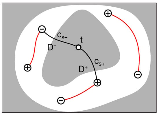
Figure 1. The definition of the positive continuity distance ($D^{+}$) and the negative continuity distance ($D^{-}$) at point t. The red lines connecting dual residues represent the discontinuity boundaries, and the black lines refer to the the shortest paths to the residues. The full (sum) continuity distance (D) in the gray areas is higher than a given threshold.

In the case that the phase retains a certain continuity among neighboring regions, the appropriate use of the continuity may make it easier to connect and merge them. The definition of the continuous region $\mathrm{\Theta }$ can be expressed as follows:

$$\mathrm{\Theta }=\{\cup (x,y\left)\right|D(x,y)\ge \gamma ,(x,y)\notin \mathrm{\Omega }\},$$

(3)

where $\mathrm{\Theta }$ refers to a continuous region and connected domain, $\gamma$ refers to the corresponding continuity distance threshold, and $\mathrm{\Omega }$ refers to areas masked for very low coherence or others. The function of the threshold $\gamma$ is to guarantee that no hidden phase discontinuity appears in continuous regions. It is worth noting that different regions might have different thresholds for better area coverage.

The continuous regions should be as large as possible once the thresholds have been set. The thresholds can be described as

$$({\gamma }_1,\cdots ,{\gamma }_n)=\underset{\gamma }{arg\max }\mathbf{\Xi },\mathbf{\Xi }=\sum _1^n{\mathrm{\Theta }}_i,$$

where $\mathbf{\Xi }$ refers to the region set. The threshold values should be as small as possible, and they could be specified by searching from small to large in the continuity distance range.

2.2. Region Residue Pairs’ Detection and Region Phase Alignment

Setting local phase references for the separated continuous regions, we can obtain the continuous unwrapped phase in each region, as cycle jumps only exist outside. Taking into account cycle jumps between the phase references, it is necessary to align the phase of all regions for a global continuity frame. Phase connections must be established between them.

2.2.1. Definitions of Region Phase Difference and Region Residue

To establish phase connections between separated continuous regions, we duplicated and propagated unwrapped phase $\mathrm{\Phi }$ within the continuous regions outward according to the principle of the minimum Euclidean distance. The mapping from a given point to its corresponding unwrapped phases within the continuous region can be described as

$$(x,y)\mapsto \underset{(u,v)}{argmin}{(x-u)}^2+{(y-v)}^2,(x,y)\notin \mathbf{\Xi },(u,v)\in \mathbf{\Xi },$$

(4)

where $(x,y)$ refers to the location of a point outside and $(u,v)$ refers to a point within regions. With the rule, the phase outside of regions can be set, such as $\mathrm{\Phi }(x,y)=\mathrm{\Phi }(u,v)$, and the areas outside (white areas in Figure 2) are divided and attached to their nearest regions. Phase connections between continuous regions depend on the phase at expanded boundaries. We denote the expanded boundary as l, shown as dashed lines in Figure 2.

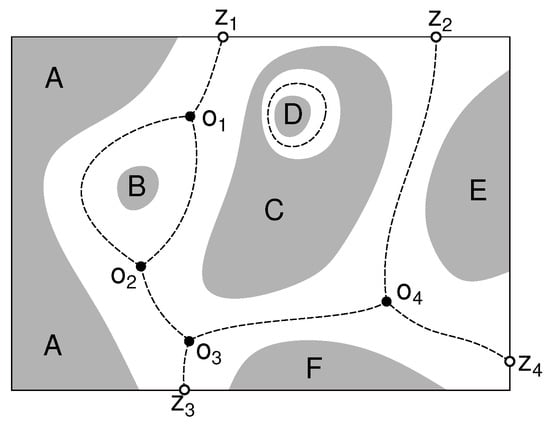
Figure 2. An example of continuous regions A, B, C, D, E, F, and their expanding boundaries (dashed lines), region corner $o_i$ ($i=1,2,3,4$) (solid circles), and border corner $z_i$ ($i=1,2,3,4$) (open circles).

The mean and variance of the expanded phase difference are calculated between continuous regions on the boundaries. For the boundary l between regions M and N, the average phase difference $\Delta {\mathrm{\Phi }}_l$ from M to N is calculated by path integrating as follows:

$$\Delta {\mathrm{\Phi }}_l=\frac{1}{\rho }{\int }_l({\mathrm{\Phi }}_N-{\mathrm{\Phi }}_M)\mathrm{d}\rho ,$$

(5)

where $\mathrm{d}\rho$ is the differential length and ${\mathrm{\Phi }}_N$ and ${\mathrm{\Phi }}_M$ refer to the expanded unwrapped phase. $\Delta {\mathrm{\Phi }}_l$ refers to the phase shift of the two regions on boundary l, whose quality can be described by the variance ${\sigma }^2$. Considering the boundary length and variance, we define a discontinuity cost index $\mathrm{\Lambda }$ as follows:

$${\mathrm{\Lambda }}_l=\frac{\rho }{{\sigma }_{\Delta \mathrm{\Phi }}^2}=\frac{{\rho }^2}{{\int }_l{({\mathrm{\Phi }}_N-{\mathrm{\Phi }}_M-\Delta {\mathrm{\Phi }}_{MN})}^2\mathrm{d}\rho }.$$

(6)

$\mathrm{\Lambda }$ describes the continuity quality of expanding boundaries and is taken as the cost of discontinuity on the boundary. However, the mean of region phase difference $\Delta {\mathrm{\Phi }}_l$ is unreliable at region boundaries with poor continuity.

Likewise, a region discontinuity index, the region residue, is defined similarly at the intersections of different expanded boundaries referred to as region corners (solid circles in Figure 2). The intersections of region boundaries and borders are called border corners (open circles in Figure 2). Assuming three boundaries or more meet at a certain point, the region residue r at the region corner is calculated as follows:

$$r=\sum _{i=1}^n\lfloor \frac{\Delta {\mathrm{\Phi }}_{l_i}}{2\pi }\rceil ,$$

(7)

where $\lfloor ·\rceil$ is the rounding operator and the sum calculation is performed clockwise (or counterclockwise). Considering the case of raster data, the value of integer n is generally 3 or 4, and the residue values are generally $\pm 1,\pm 2,\cdots$, the larger the absolute value and the smaller the probability of occurrence according to our experiments.

For example, we calculated the residue value at region corner $o_4$ in the bottom right of Figure 2, and the phase difference values on the boundaries are noted in Figure 3. The calculation is as follows:

$$r_{o_4}=\lfloor 1.6\rceil +\lfloor -0.8\rceil +\lfloor 0.2\rceil =2-1+0=+1.$$

Non-zero residue values indicate that one or more phase discontinuity boundaries exist, which might cause regional inconsistencies. It is necessary to detect possible discontinuities before using phase differences to align the region phases.

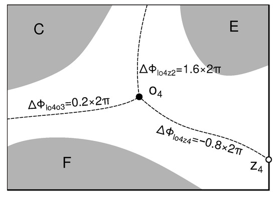
Figure 3. A region corner among continuous regions and region phase differences calculated clockwise.

We took the region corners and border corners as vertices and the region boundaries as connecting edges, which can form a graph structure (Figure 4a). A graph structure is used to illustrate the processing of region residues. Note that the closed boundaries without region corners, such as that between continuous regions C and D, are not shown in the graph, for no residue could be detected there.

2.2.2. Balancing Region Residues and Aligning Region Phases

The corners farther from residues are expected to have a higher continuity measure. Similarly, we define the continuity distance at region corner t as

$$R_t^{\pm }=min\sum {\mathrm{\Lambda }}_{l_i}|l_i\in {\mathit{L}}_s^t,s\in {\mathit{O}}^{\pm }\cup \mathit{Z}$$

(8)

where ${\mathit{O}}^{\pm }$ is the positive or negative residue set, $\mathit{Z}$ is the border corner set, and ${\mathit{L}}_s^t$ is a boundary subset connecting the reference residue s and the target corner t. The residues and border corners are taken as the source of the continuity distance, and $\mathrm{\Lambda }$ refers to the distance gain of the path sections. Taking the corners in Figure 4a as an example and assuming $\mathrm{\Lambda }$ values of each boundary and the positive residue $o_2(r=+1)$, $o_4(r=+1)$ and negative residue $o_1(r=-2)$, we calculated the positive and negative continuity distances noted as $(R^{+},R^{-})$ in Figure 4a.

In order to balance the residues, it should find the path with the minimum continuity distance ($\mathrm{\Lambda }$). The focus is on how to balance the dual residues, based on the distance map that is generated at all vertices. The ideal coupling edges $\mathit{W}$ of the dual residues is expected to minimize the objective function as follows:

$$J=\sum _{i=1}^n{\mathrm{\Lambda }}_{l_i},l_i\in \mathit{W},$$

(9)

where $l_i$ visits all elements of $\mathit{W}$ and n is the size of $\mathit{W}$. The minimization problem is N-P hard [32], and we provide an approximate solution scheme based on the corner continuity distance map.

Figure 4. A graph (a) derived from Figure 2 and its continuity distance map after the first coupling (b) and the second coupling (c). Distance values noted in the pair as $(R^{+},R^{-})$ near the vertices and $\mathrm{\Lambda }$ values noted beside the edges. Solid and open arrows indicate the positive and negative propagation, respectively.

Figure 4. A graph (a) derived from Figure 2 and its continuity distance map after the first coupling (b) and the second coupling (c). Distance values noted in the pair as $(R^{+},R^{-})$ near the vertices and $\mathrm{\Lambda }$ values noted beside the edges. Solid and open arrows indicate the positive and negative propagation, respectively.

A pair of residues can be defined as a positive and a negative residue that are sources of the continuity distance for each other. The connecting edges between the residues are marked with phase discontinuities. With a positive residue point $s_A$ and a negative residue point $s_B$, the dual pair ${\mathrm{\Gamma }}_{s_B}^{s_A}$ is expected to satisfy the following condition:

$${\mathrm{\Gamma }}_{s_B}^{s_A}:\iff {\mathrm{{\rm Y}}}_{s_B}^{+}\mapsto s_A\wedge {\mathrm{{\rm Y}}}_{s_A}^{-}\mapsto s_B,s_A\in {\mathit{O}}^{+},s_B\in {\mathit{O}}^{-},$$

(10)

where ${\mathrm{{\rm Y}}}_{s_A}^{-}$ is the source of the negative continuity distance of $s_A$ and ${\mathrm{{\rm Y}}}_{s_B}^{+}$ is the source of the positive continuity distance of $s_B$, while ↦ refers to the mapping operator. For residue pairs that need to take border corner $s_Z$ into account, the corresponding pairs ${\mathrm{\Gamma }}_{s_Z}^{s_A}$ and ${\mathrm{\Gamma }}_{s_B}^{s_Z}$ are defined as follows:

$$\begin{array}{cc}\hfill & {\mathrm{\Gamma }}_{s_Z}^{s_A}:\iff {\mathrm{{\rm Y}}}_{s_A}^{-}\mapsto s_Z,s_A\in {\mathit{O}}^{+},s_Z\in \mathit{Z}\hfill \end{array}$$

(11)

$$\begin{array}{cc}\hfill & {\mathrm{\Gamma }}_{s_B}^{s_Z}:\iff {\mathrm{{\rm Y}}}_{s_B}^{+}\mapsto s_Z,s_B\in {\mathit{O}}^{-},s_Z\in \mathit{Z}.\hfill \end{array}$$

(12)

According to the above definitions, it is convenient in Figure 4 to find region residue pairs ${\mathrm{\Gamma }}_{o_1}^{o_2}$ and ${\mathrm{\Gamma }}_{z_4}^{o_4}$ (Figure 4b). However, the residue balancing is not finished after the one time of pair detection, for residue $o_1(r=-2)$ needs more operations.

Before the next pair detecting, we need to update the vertices’ continuity distance values affected by the balanced residues. Since the $\mathrm{\Lambda }$ value of each edge for coupling in Equation (9) is counted only once, $\mathrm{\Lambda }$ on the coupling edges was set as 0 when updating the distance values. A border corner is expected to contain both positive and negative residues indefinitely. The distance values of $o_1$, $o_2$, $o_3$, and $o_4$ all were updated as shown in Figure 4b.

Because the newly detected connecting edge may overlap the previous detection, it is dealt with by strengthening in the same direction and weakening in the opposite direction. The merging result of the old and new pairs is marked in Figure 4c, showing that the edges $o_2{o}_3$ and $o_3{o}_4$ become coupled, and the edge $o_4{z}_4$ becomes uncoupled, namely

$${\mathrm{\Gamma }}_{z_4}^{o_4}\oplus {\mathrm{\Gamma }}_{o_1}^{z_4}={\mathrm{\Gamma }}_{o_1}^{o_4},$$

where ⊕ is the merging operator of the residue pairs. If all the residues are balanced after the detection of the pairs, the corresponding expanded boundaries form a discontinuity edge set $\mathit{W}$ among the regions.

The operation of aligning unwrapped phases between continuous regions is to correct the integer-cycle shift. For example, the aligned phases of the region N are as follows:

$$\overline{\mathrm{\Phi }}(x,y)=\mathrm{\Phi }(x,y)+2\pi K_N,(x,y)\in N$$

where $\mathrm{\Phi }$ refers to the unaligned unwrapped phase, $\overline{\mathrm{\Phi }}$ refers the phase after aligning, and $K_N$ is the integer-cycle offset. To align all the separate regions, one of them is set as the reference. For other regions, given the offset value of a neighboring region M and the connecting edge l, the offset of N is calculated as follows:

$$K_N=K_M+\lfloor \frac{\Delta {\mathrm{\Phi }}_l}{2\pi }\rceil ,l\notin \mathit{W},$$

(13)

where l cannot be in the discontinuity boundary set.

2.3. Region Growing Based on Heterogeneous Residual Diffusion

The proposed region growing method is based on heterogeneous residual diffusion outside of separate continuous regions, which ensures that the unwrapped phase outside regions is continuous and congruent with that inside.

2.3.1. Initializing Unwrapped Phase Outside Regions

To initialize the unwrapped phase outside of separate regions, we used the Poisson equation and the Dirichlet boundary condition. The Poisson equation is represented by

$$\begin{array}{cc}\hfill {\nabla }^2\widehat{\mathrm{\Phi }}(u,v)& ={\nabla }^2\mathrm{\Psi }(u,v),(u,v)\notin \mathbf{\Xi }\hfill \\ \hfill \widehat{\mathrm{\Phi }}(x,y)& =\overline{\mathrm{\Phi }},(x,y)\in \mathbf{\Xi },\hfill \end{array}$$

where ${\nabla }^2$ is the Laplacian operator, $\widehat{\mathrm{\Phi }}$ refers to the initial solution, ${\nabla }^2\mathrm{\Psi }$ is the Laplacian of the wrapped phase $\mathrm{\Psi }$, and $\overline{\mathrm{\Phi }}$ refers to the aligned unwrapped phases, which can guarantee a unique unwrapping phase solution, but it may not be congruent with the wrapped phases [33].

We then define a linear discontinuity indicator, which can be used to judge the existence of discontinuous boundaries in grid data. Given a horizontal or vertical line segment l, where unwrapped phases ${\overline{\mathrm{\Phi }}}_s$ and ${\overline{\mathrm{\Phi }}}_e$ are at the start and end, respectively, and wrapped phase samples, ${\mathrm{\Psi }}_i,(i=1,2,\cdots ,n)$, are distributed in sequence, we define the indicator $\kappa$ as

$${\kappa }_c={\overline{\mathrm{\Phi }}}_s-{\overline{\mathrm{\Phi }}}_e+{\sum }_{i=1}^{n+1}\mathcal{W}({\mathrm{\Psi }}_i-{\mathrm{\Psi }}_{i-1}),$$

(14)

where $\mathcal{W}(·)$ is the wrapping operator, ${\mathrm{\Psi }}_0=\mathcal{W}\left({\overline{\mathrm{\Phi }}}_s\right)$, and ${\mathrm{\Psi }}_{n+1}=\mathcal{W}\left({\overline{\mathrm{\Phi }}}_e\right)$. When $\kappa$ is non-zero, it indicates that l crosses one or more phase discontinuous boundaries, but note that opposite does not hold.

As shown in Figure 5, the linear discontinuity indicator can be used to identify areas where discontinuous boundaries exist, such as the region marked in green. Additionally, the indicator can be used to develop a decision scheme on solving for the unwrapped phase horizontally or vertically, by comparing the value of $\kappa$ for horizontal and vertical line segments. Generally, solutions obtained using the Poisson equation are preferred when $\kappa =0$, compared to those of $\kappa \ne 0$ or undefined.

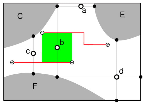
Figure 5. The linear discontinuity indicator in different cases. Horizontal ${\kappa }_x=0$ on point a, vertical ${\kappa }_y=0$ on point b, ${\kappa }_y\ne 0$ on point c, and ${\kappa }_x$ and ${\kappa }_y$ both undefined on point d. The lines in red mark two discontinuity boundaries, and the area in green defines a dangerous region.

In a more concise manner, the initial solution outside the continuous regions could be described as

$${\widehat{\mathrm{\Phi }}}^0=\left\{\begin{array}{ccc}{\widehat{\mathrm{\Phi }}}_x& & {\kappa }_x=0,{\kappa }_y\ne 0\mathrm{or}\mathrm{undefined}\hfill \\ {\widehat{\mathrm{\Phi }}}_y& & {\kappa }_y=0,{\kappa }_x\ne 0\mathrm{or}\mathrm{undefined}\hfill \\ \frac{{\widehat{\mathrm{\Phi }}}_x+{\widehat{\mathrm{\Phi }}}_y}{2}& & \mathrm{otherwise}\hfill \end{array}\right..$$

2.3.2. Heterogeneous Residual Diffusion

The proposed method utilizes the concept of residual phase $\vartheta$, defined as

$$\vartheta =\mathcal{W}(\widehat{\mathrm{\Phi }}-\mathrm{\Psi }),$$

to guide the unwrapping process. Nonlinear diffusion of the residual phase is based on heterogeneous smoothing, which heavily smooths the residual phase in the direction where the wrapped phase is smoothest. This is accomplished by employing a differential equation and a boundary condition, represented by

$$\begin{array}{c}\hfill \frac{\partial \vartheta }{\partial t}(u,v,t)={g(|\nabla \mathrm{\Psi }|}^2){\vartheta }_{\Vert }^{″}+{h(|\nabla \mathrm{\Psi }|}^2){\vartheta }_{\perp }^{″}\end{array}$$

(15)

$$\begin{array}{c}\hfill \vartheta (x,y)=0,(u,v)\notin \mathbf{\Xi },(x,y)\in \mathbf{\Xi },\end{array}$$

(16)

where ${\vartheta }_{\Vert }^{″}$ refers to the second derivative of $\vartheta$ along the tangent direction of the contour of $\mathrm{\Psi }$ and ${\vartheta }_{\perp }^{″}$ refers to the second derivative in the gradient direction that is normal to the tangent direction (as shown in Figure 6).

$$\begin{array}{cc}\hfill {\vartheta }_{\Vert }^{″}& =\frac{1}{{|\nabla \mathrm{\Psi }|}^2}\left[\begin{array}{cc}\nabla {\mathrm{\Psi }}_y& -\nabla {\mathrm{\Psi }}_x\end{array}\right]{\mathit{H}}_{\vartheta }{\left[\begin{array}{cc}\nabla {\mathrm{\Psi }}_y& -\nabla {\mathrm{\Psi }}_x\end{array}\right]}^T\hfill \\ \hfill {\vartheta }_{\perp }^{″}& =\frac{1}{{|\nabla \mathrm{\Psi }|}^2}\left[\begin{array}{cc}\nabla {\mathrm{\Psi }}_x& \nabla {\mathrm{\Psi }}_y\end{array}\right]{\mathit{H}}_{\vartheta }{\left[\begin{array}{cc}\nabla {\mathrm{\Psi }}_x& \nabla {\mathrm{\Psi }}_y\end{array}\right]}^T\hfill \end{array}$$

is used, where ${\mathit{H}}_{\vartheta }$ is the Hessian matrix of $\vartheta$, $g(·)$ is a hypersurface minimal function defined as $g\left(s\right)={(1+s)}^{-\frac{1}{2}}$, and $h\left(s\right)=g\left(s\right)+2s{g}^{\prime }\left(s\right)$.

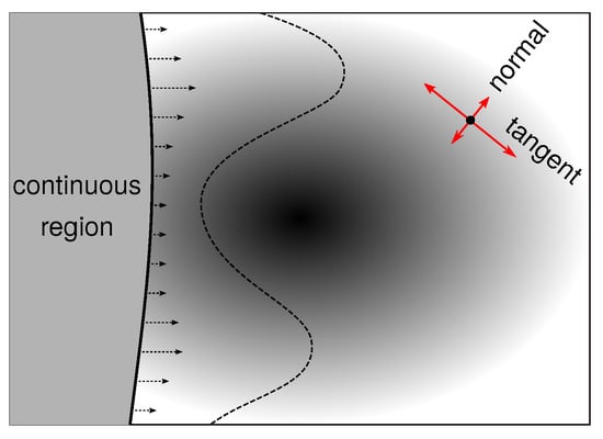
Figure 6. Nonlinear residual diffusion and region growing. The diffusion in the tangent direction of the contour is designed to be stronger than that in the normal direction, which drives regions to grow faster in flatter directions.

In nonlinear diffusion, the iterative process is represented by

$${\widehat{\mathrm{\Phi }}}^{n+1}={\widehat{\mathrm{\Phi }}}^n+{\left(g\right(|\nabla \mathrm{\Psi }|}^2){\vartheta }_{\Vert }^{″}+{h\left(\right|\nabla \mathrm{\Psi }|}^2\left){\vartheta }_{\perp }^{″}\right)\Delta t$$

(17)

where $\Delta t$ is the time interval. Iterative nonlinear diffusion with known boundaries gradually adjusts the initial unwrapped phase to fit the wrapped phase.

2.3.3. Continuous Region Growing

After obtaining the iterative solution, we made the fitted solution congruent with its original wrapped phase in regions of high quality. Specifically, we select $\widehat{\mathrm{\Phi }}(u,v)$ if it satisfies the following condition:

$$\begin{array}{c}\hfill {(x-u)}^2+{(y-v)}^2\le {\delta }^2,\left|\mathcal{W}(\widehat{\mathrm{\Phi }}(u,v)-\mathrm{\Psi }(u,v))\right|\le \tau ,(x,y)\in \mathbf{\Xi },(u,v)\notin \mathbf{\Xi },\end{array}$$

where $\delta$ represents the sampling interval, $|·|$ denotes the absolute operator, and $\tau$ is a threshold of deviation, with $\tau \in (0,\pi )$.

The resulting congruent unwrapped phase $\tilde{\mathrm{\Phi }}$ is represented by

$$\tilde{\mathrm{\Phi }}(u,v)=\widehat{\mathrm{\Phi }}(u,v)+\mathcal{W}(\mathrm{\Psi }(u,v)-\widehat{\mathrm{\Phi }}(u,v)),$$

(18)

where $(u,v)$ is considered a newly added element of the continuous regions. Through the iterative process, the continuous regions continue to expand and the outside ones shrink, until a globally consistent unwrapped phase is achieved.

3. Numerical Implementation

In the proposed method, the data were organized into three primary structures: Regular Grid, Regions, and Irregular Grid. These structures were designed to efficiently store and manipulate the data related to the phase samples, corners (region corners and border corners), and continuous regions.

The Regular Grid is the most-fundamental structure, which stores information about the wrapped phase grid, quality grid, distance grid, flag grid, source grid, discontinuity grid, unwrapped phase grid, and other elements (see Figure 7, left). The Regions structure stores information about continuous regions and includes elements such as the Regular Grid instance, region id array, region flag array, and region offset array (see Figure 7, middle). The Irregular Grid stores information related to corners and relies on both the Regular Grid and the Regions structures. It includes elements such as the Regions instance, corner id array, boundary id array, corner flag array, residue array, corner source array, corner distance array, boundary flag array, boundary cost array, boundary couple, and others (see Figure 7, right).

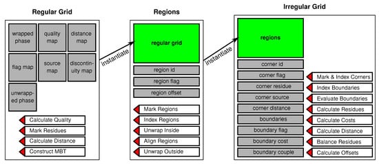
Figure 7. The main data and processing of structures Regular Grid, Regions, and Irregular Grid in the implementation.

The proposed method was implemented by extracting continuous regions, unwrapping within these regions, aligning the regions, and growing the regions. To achieve computational efficiency, a GPU-based parallel processing scheme was designed for the main processing. In this parallel mode, massive local independent operations are carried out for each local grid point, corner, boundary, and surrounding neighborhood. The main process is briefly described as follows:

• Construction of the phase continuity distance grid: the first step in constructing the phase continuity distance grid is the detection and marking of phase residues in the wrapped phase. This is followed by the calculation of the quality grid, which is defined as the inverse of the wrapped gradient variance, for example

  $$Q_x=\frac{1}{{\sigma }_x^2},Q_y=\frac{1}{{\sigma }_y^2},$$

  where ${\sigma }_x^2$ and ${\sigma }_y^2$ refer to the variance of the phase gradient in the horizontal and vertical directions. The positive and negative continuity distance grids of the wrapped phase are then calculated according to Equation (2).
  As an optional operation, the procedure constructs a preliminary minimum balanced tree (MBT) for coupling dual-phase residues and marking simple discontinuity boundaries. This step can reduce the number of unbalanced residues and simplify the distribution of the following continuous regions. The parallel calculation of the distance grid and implementation of the dual residue pair coupling in the sampling phase can be found in our previous work [31]:
• Unwrapping within the continuous regions: With the given unwrapped phase references, local direct unwrapping is performed independently in each region. The unwrapping process is based on the relations between ${\mathrm{\Phi }}_{i,j}$ and its unwrapped neighbors ${\mathrm{\Phi }}_{u,v}$ such that

  $${\mathrm{\Phi }}_{i,j}={\mathrm{\Phi }}_{u,v}+\mathcal{W}({\mathrm{\Psi }}_{i,j}-{\mathrm{\Psi }}_{u,v}),(i,j)\in \mathbf{\Xi },(u,v)\in \mathit{N}(i,j)\cap \mathbf{\Xi },$$

  where no known discontinuity boundary exists between $(i,j)$ and $(u,v)$. This process is applied to all pixels in the regions.
  If there are any neighboring phase pixels ${\mathrm{\Phi }}_i$ and ${\mathrm{\Phi }}_{i+1}$ in the continuous regions, away from known discontinuity boundaries, that meet the condition:

  $$|{\mathrm{\Phi }}_{i,j}-{\mathrm{\Phi }}_{u,v}|>\pi ,(i,j)\in \mathbf{\Xi },(u,v)\in \mathit{N}(i,j)\cap \mathbf{\Xi },$$

  a higher threshold is required as in the previous step, and the unwrapped phases are re-evaluated again.
• Continuous region boundary expansion: The local unwrapped phase in the continuous regions is expanded outwards as follows with known ${\mathrm{\Phi }}_{u,v}$, if $d_{i,j}$ is greater than $d_{u,v}+1$ or undefined:

  $${\mathrm{\Phi }}_{i,j}={\mathrm{\Phi }}_{u,v},d_{i,j}=d_{u,v}+1,(i,j)\notin \mathbf{\Xi },(u,v)\in \mathit{N}(i,j)\cap \mathbf{\Xi },$$

  where d refers to the distance to the nearest grid region. The phase difference and discontinuity cost are calculated on each boundary between the regions according to Equations (5) and (6). Region residue detection is performed on each region corner according to Equation (7).
• Corner continuity distance calculation: In order to improve the efficiency of corner continuity distance calculation, we utilized a parallel implementation of the fast march method (FMM) [34,35]. The positive and negative continuity distance of each corner point is determined through the examination of the discontinuity cost of boundaries and the distribution of region residues. The calculation is performed using known $R_u^{\pm }$, in accordance with the following equation:

  $$\begin{array}{c}\hfill s=\underset{u}{argmin}\{R_u^{\pm }+{\mathrm{\Lambda }}_l|l:i\leftrightarrow u,u\in \mathit{N}\left(i\right)\}\\ \hfill R_i^{\pm }=R_s^{\pm }+{\mathrm{\Lambda }}_{l_{si}},{\mathrm{{\rm Y}}}_i^{\pm }={\mathrm{{\rm Y}}}_s^{\pm },\end{array}$$

  where ${\mathrm{\Lambda }}_l$ represents the discontinuity cost on boundary l and $N\left(i\right)$ refers to the corner neighborhood of corner i.
• Balancing region residues: We utilized the procedure defined in Equations (10)–(12) to identify pairs of detectable residues and assigned them the appropriate continuity distance values. Subsequently, the residues and boundary indexes are adjusted in accordance with the process outlined in Algorithm 1. Here, the boundary couple index, C, takes a value of zero in the case of an uncoupled pair, and the direction index of the pair, b, is defined as $\pm 1$, depending on whether the direction of the pair and the direction of the boundary are the same.

  Algorithm 1 Balancing region residues.

  1: repeat   2:  for all unbalanced residue ri in parallel do   3:   test coupling conditions in Equations (10)–(12)   4:   if found a pair ${\mathrm{\Gamma }}_v^u$ then   5:    $r_u^{+}=r_u^{+}-1$ for Equations (10) and (11);   6:    $r_v^{-}=r_v^{-}+1$ for Equations (10) and (12);   7:    trace pair boundaries ${\mathit{L}}_v^u$;   8:    for $l_j$ in ${\mathit{L}}_v^u$ do   9:     $C_j=C_j+b$; 10:    end for 11:   end if 12:  end for 13:  update distance $R^{\pm }$ and sources ${\mathrm{{\rm Y}}}^{\pm }$; 14: until residues are all balanced.

• Aligning region phase: A reference region was chosen, and the unwrapped phase of all other regions was adjusted accordingly, using Equation (13), on boundaries without a couple for C. This resulted in the establishment of a global phase continuity framework.
• Initializing solution outside regions: The initial unwrapped phase outside the regions is obtained after detecting phase discontinuities in the horizontal and vertical directions. This was accomplished by solving the Poisson equations according to the linear discontinuities defined in Equation (14). The local Poisson equation in the horizontal or vertical direction outside the continuous regions can be written as

  $$\left[\begin{array}{ccc}-1& 2& -1\end{array}\right]{\left[\begin{array}{ccc}{\widehat{\mathrm{\Phi }}}_{i-1}& {\widehat{\mathrm{\Phi }}}_i& {\widehat{\mathrm{\Phi }}}_{i+1}\end{array}\right]}^T={\nabla }^2{\mathrm{\Psi }}_i,$$

  and the equation changes at the boundaries. For example, if $(i+1)$ is in a continuous region, the equation is rewritten as

  $$\left[\begin{array}{cc}-1& 2\end{array}\right]{\left[\begin{array}{cc}{\widehat{\mathrm{\Phi }}}_{i-1}& {\widehat{\mathrm{\Phi }}}_i\end{array}\right]}^T={\nabla }^2{\mathrm{\Psi }}_i+{\overline{\mathrm{\Phi }}}_{i+1},(i+1)\in \mathbf{\Xi }.$$
  In our GPU implementation, we employed the parallel cyclic reduction (PCR) method [36] to solve the Poisson equation.
• Heterogeneous diffusion: Heterogeneous diffusion is applied to ensure that the unwrapped phase remains congruent with the wrapped phase, in accordance with Equations (17) and (18). This process is repeated to expand the regions until the phase stabilizes and converges. The final unwrapped result is obtained once convergence is achieved. It is important to note that the time interval $\Delta t$ should not break the stability of the diffusion process, and we set $\Delta t<\frac{1}{4}$ in our implementation.

The above-described main steps of the algorithms were implemented in a parallel manner utilizing the capabilities of GPU devices. A simplified representation of the entire process is presented in Figure 8.

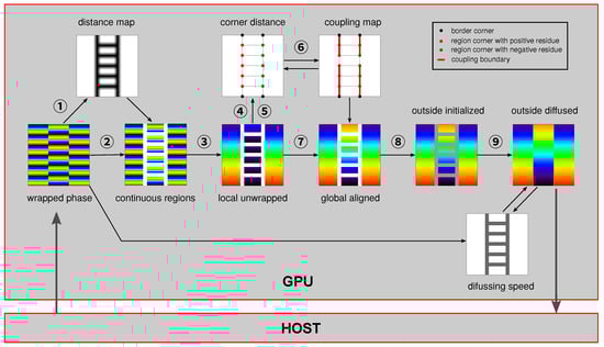
Figure 8. A simple demonstration of the processing flow for the proposed PU method based on separated continuous regions.

4. Experiments and Analysis

We chose to validate the efficiency and reliability of the proposed PU method using three real interferograms acquired by TanDEM-X satellites. The choice to test the method on TanDEM-X data was motivated by the unique characteristics of the satellite’s data acquisition, which include the ability to collect high-resolution data from a variety of geographical regions and the ability to capture phase information with a high degree of accuracy.

The first interferogram covers the city of Wuhan, China, in 2011, and the observed area includes rivers and lakes, which result in separated regions with a high-quality local phase. Observations of Singapore, which cover the sea and several separate islands, comprised the second set of experimental data. The third experimental data came from observations of Songshan, China, and the observing area included undulating hills, which resulted in shadows and overlapping in the data. The experiments were carried out on a machine equipped with a CPU (8 cores, 2.70 GHz), a GPU (NVIDIA Quadro M2000M, 640 cores, 1.03 GHz) with 4 GB of device memory (1.25 GHz), a 16 GB host memory (dual-channel, DDR4, 2133 MHz), and a 64-bit operating system.

The three experimental interferograms were of $2944\times 5014$ pixels, $1752\times 2984$ pixels, and $2073\times 3529$ pixels, respectively. There were 72,751 positive and 73,183 negative, 13,178 positive and 13,151 negative, and 86,080 positive and 86,093 negative phase residues detected in the three interferograms, respectively (Figure 9a–c). The initial distance maps were constructed based on these positive and negative residues (Figure 9d–f), and the coupling of residue pairs was performed four times for each of the three datasets. This process resulted in 10,094 pairs being found and 79 positive and 11 negative phase residues remaining uncoupled in the Wuhan data, 14,895 pairs and 193 positive and 153 negative residues remaining uncoupled in the Singapore data, and 82,719 pairs and 3718 positive and 3690 negative residues remaining uncoupled in the Songshan data.

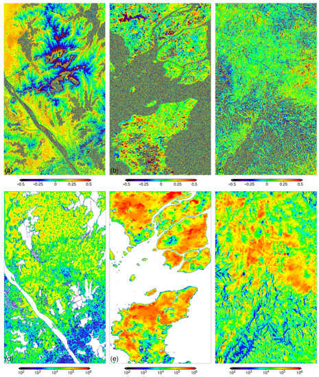
Figure 9. The wrapped phases (number of $2\pi$) from Wuhan (a), Singapore (b), and Songshan (c) and their phase distance maps (d–f) after four times of residue coupling, respectively. The water areas in (d,e) are masked.

The maximum values in the distance maps, $D_{max}$, were 192,475, 3,013,342, and 128,245, respectively, and the initial ratio thresholds for region extraction were set at 0.1%, 0.1%, and 1.0%. The step interval was set at 0.1%, and the stop thresholds were 0.8%, 0.3%, and 1.9%, correspondingly. The extraction yielded 7504 continuous regions for the interferogram of Wuhan, 552 continuous regions for the interferogram of Singapore, and 7246 continuous regions for the interferogram of Songshan. The coverage percentage of extracted regions in the valid areas was 84.10, 87.64, and 53.87, respectively. These values are listed in Table 1.

Table 1. Statistics of continuous region extraction on the experimental data.

Data	${\mathit{D}}_{\mathit{max}}$	${\mathit{\gamma }}_0$ (%)	$\mathit{\delta }\mathit{\gamma }$ (%)	${\mathit{\gamma }}_1$ (%)	Regions	Coverage (%)
Wuhan	192,475	0.1	0.1	0.8	7504	84.10
Singapore	3,013,342	0.1	0.1	0.3	552	87.64
Songshan	128,245	1.0	0.1	1.9	7246	53.87

A detailed analysis of the iterative extraction process of the Wuhan data is presented in Figure 10. As the threshold increased, it was observed that the corresponding detection area gradually decreased, and the extracted continuous region gradually became larger. It is noted that a higher threshold may decompose a large region into more small regions, resulting in an increase in the number of regions.

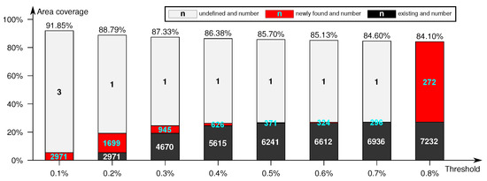
Figure 10. Area coverage and number of changes of regions of the Wuhan data in the iterative extracting process.

Using local phase references, direct unwrapping was performed in each region. Next, the unwrapped phase of the reliability regions was expanded to generate boundaries between regions. The numbers of boundaries with and without corners, as well as the number of corners were calculated for each of the three data, as shown in Table 2.

Table 2. Number statistics of boundaries, corners, residues, and pairs in the experimental data.

Data	Bound${}_{\mathit{a}}$	Bound${}_{\mathit{b}}$	Corner	${\mathit{r}}_{+1}$	${\mathit{r}}_{-1}$	${\mathit{r}}_{+2}$	${\mathit{r}}_{-2}$	${\mathit{r}}_{\mathit{other}}$	Pair
Wuhan	19,253	526	12,890	188	182	2	5	0	192
Singapore	1402	35	973	96	95	2	1	0	105
Songshan	20,298	200	13,762	1004	997	9	11	0	1054

Bound_a is for the boundaries with corners, Bound_b for the boundaries without corners, and r_other for the residues greater than 2 or less than −2.

Region residue detection was then performed at the intersection of these boundaries, with the results being recorded for each of the three data. After iteratively constructing corner reliability maps and performing residue coupling (4, 6, and 6 times), the number of pairs of unbalanced residues was determined for each interferogram, as shown in Table 2. The number of unbalanced residues in each coupling iteration is presented in Figure 11.

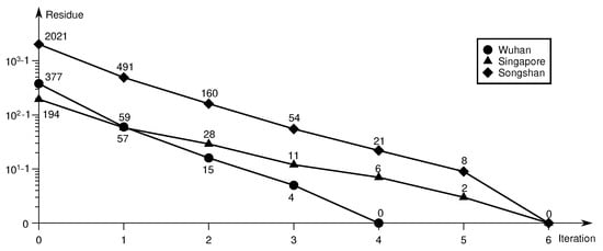
Figure 11. Numbers of unbalanced residues in the coupling iterations in the experimental data.

In the detail of Figure 12, the phase in Regions A and B varied greatly, resulting in Positive Residues 1 and 2 and Negative Residues 3 and 4. After residue coupling, the marked discontinuity boundaries changed the phase cycle of Areas B, C, and D, which is a typical process of residue coupling and phase alignment. Region E, with an extreme phase change, had different effects on the upper and lower regions.

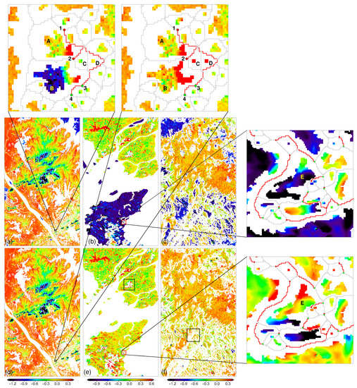
Figure 12. The local unwrapped phase in the continuous regions for Wuhan (a), Singapore (b), and Songshan (c) and their global aligned versions in (d–f), respectively. Details of windowed areas with boundaries (black), residues (red for positive, green for negative), and coupling edges (red).

After aligning the regions for the global frame, Poisson solving with the Dirichlet boundary condition provided the initial unwrapped phase, considering the discontinuities defined in Equation (14). The initial solutions were obtained from four times of PCR iterative solving with wrapped phase differences along the horizontal and vertical directions. The three initial solutions were then subjected to 1000 iterations of nonlinear diffusion, respectively. Congruent areas were updated every 20 iterations with $\tau =0.05$ for the data of Wuhan, $\tau =0.12$ for the data of Singapore, and $\tau =0.05$ for the data of Songshan. The initial unwrapped phase from PCR solving and the final results from nonlinear diffusing are shown in Figure 13.

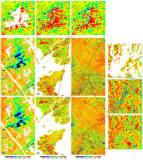
Figure 13. The initial unwrapped phase outside the continuous regions from PCR for Wuhan (a), Singapore (b), and Songshan (c) and their final version (d–f) with 1000 times of nonlinear diffusion, respectively. The detailed local unwrapped phase in the regions shows the unwrapped version and diffusion version of the areas marked.

In order to provide further insight into the processing, two windowed areas of 250 × 250 pixels and 350 × 350 pixels were analyzed in detail. Initial solutions filled the areas outside the continuous regions, and the continuity of the phase between outside and inside the continuous regions was preserved. However, it is noted that stripes appeared in areas with severe noise, which was caused by the integration path passing through phase discontinuity boundaries. The final results from nonlinear diffusion made effective corrections in the areas with stripes. Some small pits appeared in the areas with severe noise, which was attributed to the attenuation of the smoothing effect of nonlinear diffusion in these noise-affected areas, where the effect of guidance from the wrapped gradient was not reliable.

To further evaluate the effectiveness of the proposed method, we calculated the wrapped phase differences between the unwrapped and original wrapped phases. This quantity provides insight into the impact of the unwrapping process, specifically the removal of cycle jumps. As shown in Figure 14, the residual phase maps revealed that the proposed method effectively completed the unwrapping process, as evidenced by the minimal and scattered residual phases after masking out water bodies in the Wuhan and Singapore data. The roots of variance of the residuals in the results were 0.0343, 0.0470, and 0.0928, respectively. The area coverage of residual absolute values larger than 0.012 were 1.951%, 2.545%, and 9.672%. However, it is noted that the relatively high number of residual phases in the Songshan region was a result of strip-shaped shadows or layovers caused by steep mountainous terrain. Despite the use of a smoothing procedure using nonlinear diffusion, the traces of the discontinuity boundaries could not be fully eliminated.

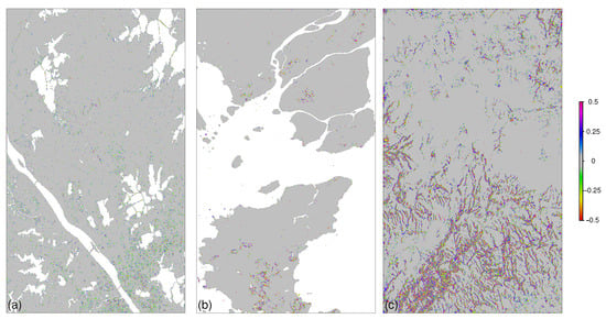
Figure 14. The wrapped phase difference between our diffused results and the wrapped phase for the data of Wuhan (a), Singapore (b), and Songshan (c).

We compared the performance of our proposed method with several existing unwrapping methods, including SNAPHU [10], region growing [6], GAMMA minimum cost flow (MCF), and PHASS [37,38] by processing the same dataset (as illustrated in Figure 15). The SNAPHU method and GAMMA method employ similar optimization schemes based on network flow, while the region growing method utilizes a growing scheme that relies on reliability sorting. For SNAPHU, we utilized the DEFO mode with coherence as the weight and used the final solution. For the region growing method, we used the pixel-level reliability to connect different growing regions. For the GAMMA method, we used the minimum cost flow algorithm to minimize the cycle errors. For the PHASS method, graph optimization algorithms based on MCF with regions were employed.

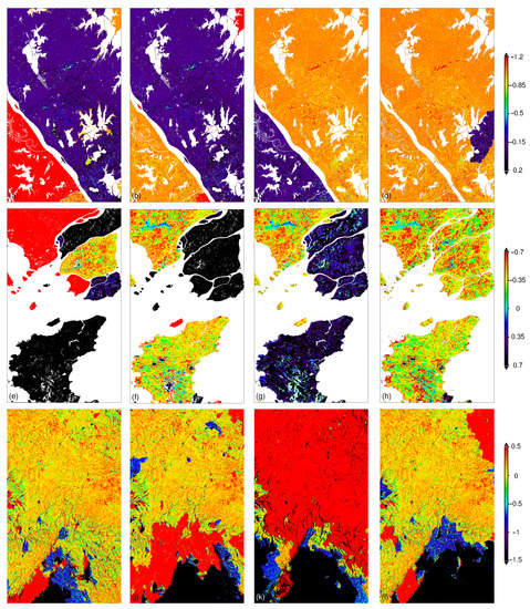
Figure 15. The wrapped phase for the experimental data of Wuhan (a–d), Singapore (e–h), and Songshan (i–l) from the SNAPHU, region growing, GAMMA, and PHASS PU methods.

The results of the unwrapping process indicated that SNAPHU performed well in the Wuhan and Singapore cases within land areas. However, SNAPHU’s connection processing between regions was poor, resulting in cycle jumps between regions. The region growing method, on the other hand, focuses on connecting different growing regions at pixel-level continuity, but the instability of the noisy areas resulted in different cycle deviation patches. The GAMMA method showed similar results with cycle errors among separated regions. Despite the small area of error, the PHASS method gave better results on the Wuhan and Singapore data, but it performed poorly on the Songshan data. For the Songshan case, SNAPHU, region growing, GAMMA, and PHASS all failed to produce a global continuity solution across noisy areas.

We conducted an analysis of the runtime costs in our PU experiments (as shown in Table 3). On the data experiments of Wuhan and Singapore, the PHASS method spent the least time, mainly due to its low coherence region masking and CPU parallel acceleration. The times of our method were close to the PHASS method on the two data. On the Songshan data, our method significantly took the shortest time.

Table 3. Runtime (sec) cost of the five different PU methods.

Data	SNAPHU	Region Growing	GAMMMA	PHASS	Proposed
Wuhan	98.072	85.919	73.510	67.049	70.695
Singapore	86.992	27.809	64.580	23.046	23.324
Songshan	93.014	56.511	161.610	43.068	35.997

A further examination of the time costs of each processing step in our proposed method revealed that, in the Wuhan data experiment, 70.695 s were spent, with 15.8% of that time allocated to constructing the distance map, 15.4% to extracting the continuous region, 3.2% to aligning regions, and 65.6% to solving outside of regions (Table 4). In the Singapore data experiment, 3.809 s, 0.838 s, 0.555 s, and 18.122 s were spent on these steps, respectively. Similarly, in the Songshan experiment, 7.858 s, 6.456 s, 1.453 s, and 20.230 s were allocated to these steps, respectively. We observed that more than half of the total runtime was spent solving outside regions in all three experiments.

Table 4. Runtime (%) of four steps in the proposed method.

Data	Constructing Map	Extracting Regions	Aligning Regions	Solving Outside
Wuhan	15.8%	15.4%	3.2%	65.6%
Singapore	16.3%	3.6%	2.4%	77.7%
Songshan	21.8%	17.9%	4.1%	56.2%

5. Discussion

While the proposed unwrapping method was able to achieve globally consistent results in our experiments, there are still some aspects that need further discussion. One of these is the use of phase residue MBT coupling during the construction of the continuity distance map as a preprocessing step. This step effectively reduces the number of phase residues and generates a distance map with larger continuous regions. However, it is imperative to note that more coupling iterations may not always produce better results. In some cases, excessive coupling may lead to incorrect results, which highlights the importance of careful consideration when determining the optimal number of iterations.

Another issue that needs to be addressed is the relatively high processing time required for unwrapping outside regions. Improving the efficiency of this aspect of the method should be a focus of future research. This may involve modifying or replacing the proposed nonlinear diffusion technique, particularly if strict adherence to discontinuity boundaries is necessary. Additionally, the setting of the congruity parameter $\tau$ plays a significant role in both the speed of region growing and the location of discontinuity boundaries. A larger value of $\tau$ relaxes the congruity residuals, which improves efficiency, but also increases the likelihood of the convergent regions expanding across the true discontinuity boundary, resulting in an incorrect boundary location. On the other hand, a smaller value of $\tau$ results in more accurate discontinuity boundaries, but may prevent the expansion of regions, requiring a longer convergence time or even preventing convergence altogether. Through our experiments, we found that the value of $\tau$ should be around 0.1 cycles according to our empirical analysis.

6. Conclusions

In this paper, a novel unwrapping method based on separate continuous regions was proposed to address the PU problem of regions separated by noise while neighboring continuity cannot be guaranteed. The proposed method was based on a continuity distance measure, which is computed as the minimum weighted distance from the dual-phase residues. Distance thresholds are used to identify regions with good phase continuity, which enables correct unwrapping in local regions. By assuming phase continuity between regions, the unwrapped phase of the region is expanded to calculate cycle numbers and continuity quality between regions. The region residues are detected using shift numbers. The coupling of region residues is designed to identify region discontinuities, which are considered during constructing the global continuity framework. The proposed method also employs Poisson solving and nonlinear diffusion to solve outside the unwrapped regions.

The proposed method effectively addresses the issue of continuous region isolation caused by noise, by using the coupling of region residues to ensure the reliability of the phase alignment of separated regions. Additionally, the method is easily implemented in parallel, which can significantly improve the efficiency of unwrapping processing. The results of the experiments conducted on real InSAR data demonstrated the reliability and efficiency of the developed method. This method was able to overcome the limitations of prior unwrapping methods, which were seen as less reliable when dealing with regions separated by noise. The proposed method is a step forward in the field of InSAR data unwrapping. It is expected to have a positive impact on a wide range of applications that depend on InSAR data.

References

- Ghiglia, D.C.; Pritt, M.D. Two-Dimensional Phase Unwrapping: Theory, Algorithms, and Software; Wiley: Hoboken, NJ, USA, 1998. [Google Scholar]
- Yu, H.; Lan, Y.; Yuan, Z.; Xu, J.; Lee, H. Phase Unwrapping in InSAR: A Review. IEEE Geosci. Remote Sens. Mag. 2019, 7, 40–58. [Google Scholar] [CrossRef]
- Xu, W.; Cumming, I. A region-growing algorithm for InSAR phase unwrapping. IEEE Trans. Geosci. Remote Sens. 1999, 37, 124–134. [Google Scholar] [CrossRef]
- Karsa, A.; Shmueli, K. SEGUE: A Speedy rEgion-Growing Algorithm for Unwrapping Estimated Phase. IEEE Trans. Med Imaging 2019, 38, 1347–1357. [Google Scholar] [CrossRef] [PubMed]
- Ojha, C.; Manunta, M.; Pepe, A.; Paglia, L.; Lanari, R. An innovative region growing algorithm based on Minimum Cost Flow approach for Phase Unwrapping of full-resolution differential interferograms. In Proceedings of the 2012 IEEE International Geoscience and Remote Sensing Symposium, Munich, Germany, 22–27 July 2012; pp. 5582–5585. [Google Scholar] [CrossRef]
- Herráez, M.A.; Burton, D.R.; Lalor, M.J.; Gdeisat, M.A. Fast two-dimensional phase-unwrapping algorithm based on sorting by reliability following a noncontinuous path. Appl. Opt. 2002, 41, 7437–7444. [Google Scholar] [CrossRef] [PubMed]
- Xie, X.; Zeng, Q. Multi-baseline extended particle filtering phase unwrapping algorithm based on amended matrix pencil model and quantized path-following strategy. J. Syst. Eng. Electron. 2019, 30, 78–84. [Google Scholar] [CrossRef]
- Dudczyk, J.; Kawalec, A. Optimizing the Minimum Cost Flow Algorithm for the Phase Unwrapping Process in SAR Radar. Bull. Pol. Acad. Sci. Tech. Sci. 2014, 62, 511–516. [Google Scholar] [CrossRef]
- Huang, Q.; Zhou, H.; Dong, S.; Xu, S. Parallel Branch-Cut Algorithm Based on Simulated Annealing for Large-Scale Phase Unwrapping. IEEE Trans. Geosci. Remote Sens. 2015, 53, 3833–3846. [Google Scholar] [CrossRef]
- Chen, C.; Zebker, H. Phase unwrapping for large SAR interferograms: Statistical segmentation and generalized network models. IEEE Trans. Geosci. Remote Sens. 2002, 40, 1709–1719. [Google Scholar] [CrossRef]
- Sawaf, F.; Tatam, R.P. Finding minimum spanning trees more efficiently for tile-based phase unwrapping. Meas. Sci. Technol. 2006, 17, 1428. [Google Scholar] [CrossRef]
- Dong, J.; Zhuo, Z.; Li, J.; He, Y. A new phase image reconstruction method using Markov random fields. In Proceedings of the 2017 IEEE/ACIS 16th International Conference on Computer and Information Science (ICIS), Wuhan, China, 24–26 May 2017; pp. 1–5. [Google Scholar] [CrossRef]
- Xu, J.; An, D.; Huang, X.; Wang, G. Phase Unwrapping for Large-Scale P-Band UWB SAR Interferometry. IEEE Geosci. Remote Sens. Lett. 2015, 12, 2120–2124. [Google Scholar] [CrossRef]
- Zhang, Y.; Xing, Z. A Hybrid Phase Unwrapping Algorithm Based on Quality-Guided and Surface-Fitting. In Proceedings of the 2018 IEEE International Workshop on Electromagnetics: Applications and Student Innovation Competition (iWEM), Nagoya, Japan, 29–31 August 2018; pp. 1–2. [Google Scholar] [CrossRef]
- Zhang, Y.; Xing, Z. A Phase Unwrapping Algorithm Based on Branch-cut and B-Spline Fitting in InSAR. In Proceedings of the 2018 IEEE International Conference on Signal Processing, Communications and Computing (ICSPCC), Hong Kong, China, 14–16 September 2018; pp. 1–3. [Google Scholar] [CrossRef]
- Yu, H.; Lee, H. A convex hull algorithm based fast large-scale two-dimensional phase unwrapping method. In Proceedings of the 2017 IEEE International Geoscience and Remote Sensing Symposium (IGARSS), Fort Worth, TX, USA, 23–28 July 2017; pp. 3824–3827, ISSN 2153-7003. [Google Scholar] [CrossRef]
- Yu, H.; Lan, Y.; Xu, J.; An, D.; Lee, H. Large-Scale L0-Norm and L1-Norm 2-D Phase Unwrapping. IEEE Trans. Geosci. Remote Sens. 2017, 55, 4712–4728. [Google Scholar] [CrossRef]
- Zhang, Y.; Zhang, S.; Gao, Y.; Li, S.; Jia, Y.; Li, M. Adaptive Square-Root Unscented Kalman Filter Phase Unwrapping with Modified Phase Gradient Estimation. Remote Sens. 2022, 14, 1229. [Google Scholar] [CrossRef]
- Gao, Y.; Tang, X.; Li, T.; Lu, J.; Li, S.; Chen, Q.; Zhang, X. A Phase Slicing 2-D Phase Unwrapping Method Using the L 1 -Norm. IEEE Geosci. Remote Sens. Lett. 2022, 19, 1–5. [Google Scholar] [CrossRef]
- Li, H.; Zhong, H.; Ning, M.; Zhang, P.; Tang, J. Using neural networks to create a reliable phase quality map for phase unwrapping. Appl. Opt. 2023, 62, 1206. [Google Scholar] [CrossRef] [PubMed]
- Zhou, L.; Yu, H.; Lan, Y. Deep Convolutional Neural Network-Based Robust Phase Gradient Estimation for Two-Dimensional Phase Unwrapping Using SAR Interferograms. IEEE Trans. Geosci. Remote Sens. 2020, 58, 4653–4665. [Google Scholar] [CrossRef]
- Li, L.; Zhang, H.; Tang, Y.; Wang, C.; Gu, F. InSAR Phase Unwrapping by Deep Learning Based on Gradient Information Fusion. IEEE Geosci. Remote Sens. Lett. 2022, 19, 1–5. [Google Scholar] [CrossRef]
- Zhao, J.; Liu, L.; Wang, T.; Wang, X.; Du, X.; Hao, R.; Liu, J.; Liu, Y.; Zhang, J. VDE-Net: A two-stage deep learning method for phase unwrapping. Opt. Express 2022, 30, 39794. [Google Scholar] [CrossRef] [PubMed]
- Pu, L.; Zhang, X.; Zhou, Z.; Li, L.; Zhou, L.; Shi, J.; Wei, S. A Robust InSAR Phase Unwrapping Method via Phase Gradient Estimation Network. Remote Sens. 2021, 13, 4564. [Google Scholar] [CrossRef]
- Sawaf, F.; Groves, R.M. Phase discontinuity predictions using a machine-learning trained kernel. Appl. Opt. 2014, 53, 5439–5447. [Google Scholar] [CrossRef] [PubMed]
- Wu, Z.; Wang, T.; Wang, Y.; Wang, R.; Ge, D. Deep-Learning-Based Phase Discontinuity Prediction for 2-D Phase Unwrapping of SAR Interferograms. IEEE Trans. Geosci. Remote Sens. 2022, 60, 1–16. [Google Scholar] [CrossRef]
- Spoorthi, G.E.; Gorthi, S.; Gorthi, R.K.S.S. PhaseNet: A Deep Convolutional Neural Network for Two-Dimensional Phase Unwrapping. IEEE Signal Process. Lett. 2019, 26, 54–58. [Google Scholar] [CrossRef]
- Sica, F.; Calvanese, F.; Scarpa, G.; Rizzoli, P. A CNN-Based Coherence-Driven Approach for InSAR Phase Unwrapping. IEEE Geosci. Remote Sens. Lett. 2022, 19, 1–5. [Google Scholar] [CrossRef]
- Zhou, L.; Yu, H.; Lan, Y.; Xing, M. Deep Learning-Based Branch-Cut Method for InSAR Two-Dimensional Phase Unwrapping. IEEE Trans. Geosci. Remote Sens. 2022, 60, 1–15. [Google Scholar] [CrossRef]
- Li, H.; Zhong, H.; Zhang, P.; Ning, M.; Tang, J. Two-Dimensional Phase Unwrapping Based on Residual Prediction Neural Network. IEEE Geosci. Remote Sens. Lett. 2023, 20, 1–5. [Google Scholar] [CrossRef]
- Gao, J.; Sun, Z. Phase unwrapping method based on parallel local minimum reliability dual expanding for large-scale data. J. Appl. Remote Sens. 2019, 13, 038506. [Google Scholar] [CrossRef]
- Chen, C.W.; Zebker, H.A. Two-dimensional phase unwrapping with use of statistical models for cost functions in nonlinear optimization. JOSA A 2001, 18, 338–351. [Google Scholar] [CrossRef] [PubMed]
- Lyuboshenko, I.V.; Maitre, H.; Maruani, A. Least-mean-squares phase unwrapping by use of an incomplete set of residue branch cuts. Appl. Opt. 2002, 41, 2129–2148. [Google Scholar] [CrossRef]
- Capozzoli, A.; Curcio, C.; Liseno, A.; Savarese, S. A comparison of Fast Marching, Fast Sweeping and Fast Iterative Methods for the solution of the eikonal equation. In Proceedings of the 2013 21st Telecommunications Forum Telfor (TELFOR), Belgrade, Serbia, 26–28 November 2013; pp. 685–688. [Google Scholar]
- Jeong, W.K.; Whitaker, R.T. A Fast Iterative Method for Eikonal Equations. SIAM J. Sci. Comput. 2008, 30, 2512–2534. [Google Scholar] [CrossRef]
- Swarztrauber, P.N. The Methods of Cyclic Reduction, Fourier Analysis and the FACR Algorithm for the Discrete Solution of Poisson’s Equation on a Rectangle. SIAM Rev. 1977, 19, 490–501. [Google Scholar] [CrossRef]
- Tophu. Available online: https://github.com/opera-adt/tophu (accessed on 16 January 2023).
- isce-framework/isce3: InSAR Scientific Computing Environment. Available online: https://github.com/isce-framework/isce3 (accessed on 16 January 2023).
Disclaimer/Publisher’s Note: The statements, opinions and data contained in all publications are solely those of the individual author(s) and contributor(s) and not of MDPI and/or the editor(s). MDPI and/or the editor(s) disclaim responsibility for any injury to people or property resulting from any ideas, methods, instructions or products referred to in the content. |
© 2023 by the authors. Licensee MDPI, Basel, Switzerland. This article is an open access article distributed under the terms and conditions of the Creative Commons Attribution (CC BY) license (https://creativecommons.org/licenses/by/4.0/).