Abstract
The magnetotelluric method has been used to fully study regional electrical conductivity structures in different areas in mainland China; however, there is a lack of overall understanding of the electrical structure distribution. A novel insight for the study of continental-scale underlying conductivity structures was proposed in this work via geomagnetic data recorded by permanent stations. To study the underlying electrical structure distribution in mainland China, we mapped the conductors and resistors at a depth range of 4–100 km beneath mainland China using Parkinson vectors through magnetic transfer function. Three-component geomagnetic data within a low artificial disturbance period (local time 23:00–05:00) from 98 stations in 2019 were collected and processed to derive Parkinson vectors in the frequency band of 0.001–0.5 Hz. The distribution of subsurface electrical structures at distinct depths was constructed using corresponding frequency through the skin depth. We compare the consistent results herein with previous magnetotelluric studies, which indicated the reliability of our method. Combining previous multiple geophysical inversion results, we found that large-scale plastic bodies are distributed along the east of the Qinghai-Tibet Plateau and extend to the west of Yunnan. In central mainland China, the areas are mainly highly resistive, indicating that the structures are overall rigid. In north China, there exist high-low-high-low conductive structures from west to east. The separate high- and low-conductive electrical bodies in the North China Craton provide geophysical evidence that the Craton is composed of multiple blocks. The distributions of the underlying electrical structures in this work can provide an overall perspective for studying tectonic evolution and geodynamics in mainland China.
1. Introduction
The magnetotelluric (MT) method is an effective method for investigating the electrical conductivity of the Earth’s interior. In mainland China, the MT method has been widely applied to survey the distribution of regional underlying electrical conductors and resistors [,,,,,,,,,,,,,]. Xiao et al. [] found a relatively high-conductivity layer in the middle-lower crust at depths of approximately 10–100 km in the northeastern part of the Qinghai-Tibet Plateau (QTP). Bai et al. [] constructed four MT profiles utilizing 325 sites within a total length of 2110 km and found high-conductivity zones at depths of 10–100 km in the eastern QTP. Ye et al. [] revealed an upper and mid-crustal low resistive body above a depth of 10–30 km in the southeastern QTP and western Yunnan by inversing a crustal resistivity model using MT data collected from 170 sites. These studies demonstrate that, from north to south, high-conductivity layers exist in different areas of the eastern QTP. In southwest China, a high-resistivity belt [] and a resistive block [] were found based on MT profiles over 1000 km. In addition, fault zone conductors and lower crust conductivity structures were revealed in southwest China utilizing two profiles of approximately 250 km []. In northern China, the complicated North China Craton has become a focal area of current research on the underlying electrical layers using the MT method [], where resistors [,] and conductors [,,] have been studied. The locations of underlying electrical structures by the MT method mentioned above are shown in Figure 1. MT can provide lateral and vertical inversion slices to indicate electrical bodies and is mainly utilized to study tectonic evolution [], geodynamic processes [], and earthquake triggers [] of the interior Earth. The above studies have reported many electrical conductivity structures in different regions, but there is a lack of continental-scale electrical structure distribution in mainland China []. Furthermore, for data collection, the MT sites can only be sited within a broad corridor of hundreds or even thousands of kilometers in length of the profile lines, which requires substantial field work []. Alternatively, geomagnetic data can be another option to study underlying conductivity structures.
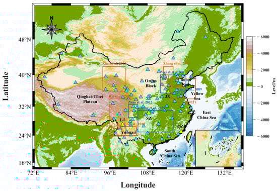
Figure 1.
The locations of the permanent magnetic stations (the blue triangles) in mainland China. The yellow triangles denote the QZ, LJ, SZ, and JX station, which are utilized to display sounding curves. Squares are the locations of study areas for previous underlying electrical conductivity structures investigations. The red and blue squares denote the study areas where scientists found high conductivity and resistivity zones, respectively [,,,,,,,,,,].
Typically, geomagnetic fields observed by ground-based magnetometers contain multiple factors besides the Earth’s main field [], including solar activity [,,], ground vibrations [,,], and underground conductive structures effect [,,]. The short-term changes in the three geomagnetic components X (north-south), Y (east-west), and Z components (or H (horizontal), D (declination), and Z (vertical) components) tend to be confined to a plane called the preferred plane []. The plane will be almost horizontal if strata are the horizontal layers, but it is sometimes tilted due to the asymmetrically induced currents owing to oceans or regional underlying conductivity structures []. The reverse inclination of the plane reflects the direction of the underlying conductivity structure, and a larger dip of the plane indicates a greater difference in conductivity []. To indicate the inclination of the plane, the Parkinson vector was proposed to point toward high-conductivity electrical structures [,]. The direction of the vectors indicates highly conductive areas and their magnitude reflects the electrical difference []. The vectors depend on the frequency and can be calculated at specific frequency bands through the magnetic transfer function [,]. Generally, Parkinson vectors are utilized to study two aspects. On the one hand, they are utilized to study the geomagnetic coast effect []. The Parkinson vectors at the coastal observatories point toward the ocean and are almost perpendicular to the coastline, which indicates that the conductivity of the ocean is higher than that of the inland continent. Typically, the further the station is from the coastline to the inland, the weaker the impact of the geomagnetic coast effect []. This effect has been observed in many countries worldwide [,,,,]. On the other hand, the Parkinson vectors are utilized to study the distribution of underlying electrical conductivity structure in inland areas, such as sharp lateral discontinuities in central Argentina Alicia [], a high-conductivity layer in northern China [], and two conductors beneath western Junggar and southwestern Chinese Altaids []. In addition, the temporal variations of Parkinson vectors have drawn the attention of scientists in recent years [,,].
The Parkinson vector is an alternative indicator for mapping the distribution of conductors or resistors. Its advantage is that instead of deploying thousands of kilometers of MT profiles, we can use permanent geomagnetic observatories to investigate underlying electrical bodies. In mainland China, three-axis fluxgate magnetometers with a sampling interval of one second are installed at almost 100 permanent geomagnetic stations to monitor daily geomagnetic fields (the north-south (X), east-west (Y), and vertical components (Z)). The geomagnetic station network provides a good opportunity to study the continental-scale underlying electrical structures. In this study, we utilized geomagnetic data collected from 98 permanent stations in the Geomagnetic Network of China in 2019 (Figure 1) to investigate the large-scale spatial distribution of underlying conductivity structures by Parkinson vectors.
2. Methodology and Results
The magnetic transfer function [,] describes the relationship between the horizontal and vertical components in the geomagnetic field, which can be written as,
X(f), Y(f), and Z(f) are the north-south, east-west, and vertical components of the geomagnetic data at a particular frequency band f, respectively. A(f) and B(f) are coefficients of the magnetic transfer function. We computed X(f), Y(f), and Z(f) utilizing a moving window of 180 min in step of one minute. A(f) and B(f) are calculated from X(f), Y(f), and Z(f) utilizing least square method. Note that A(f) and B(f) comprise the real parts Ar(f) and Br(f) and the imaginary parts of Au(f) and Bu(f), which can be written as follows,
The three times the standard deviations of Ar(f) and Br(f) are computed and determined as the thresholds. Ar(f) and Br(f) are utilized to define and compute the Parkinson vectors; their absolute values are smaller than the thresholds for the mitigation of unwanted interference owing to sudden perturbations. The Parkinson vector is defined by the azimuth PA(f) and magnitude PM(f), and they can be calculated by Ar(f) and Br(f), respectively, using the following formulas,
The azimuth distribution during the study period is constructed by utilizing the entire PA(f) with 36 angle bins at 360° with an interval of 10° []. The major distribution of the azimuths (PAmajor) is considered to be the long-term direction of the Parkinson vectors at one station which reflect the electrical conductivity structures or geomagnetic coast effect because the underlying structures are generally considered to be unchanged within one year. PM(f) with PA(f), which is distributed within the bin of PAmajor, is selected, and the major distribution value of the selected PM(f) is determined as PMmajor, which reflects the electrical difference at deep depths. We used data from the QZ station in Figure 1 as an example to demonstrate the processes for retrieving PAmajor and PMmajor. Geomagnetic data between 23:00 and 5:00, local time, were chosen to mitigate the influence of artificial noise. Figure 2a shows the one-day (i.e., 1 January 2019) raw three-component geomagnetic data at QZ station. The red line indicates the low artificial noise period (i.e., local time (LT) 23:00–05:00) data that were utilized in this study. Figure 2b shows the sounding curves using data by LT 23:00–05:00 and the other period. We can see the errors are smaller in the time period of LT 23:00–05:00 than in the other period.
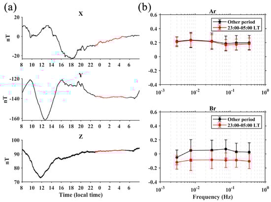
Figure 2.
(a) The raw geomagnetic X, Y, and Z component at QZ station on 1 January 2019. Red lines indicated the low artificial noise period (i.e., local time 23:00–05:00) data that are utilized in this study; and (b) sounding curves for time periods on local time 23:00–05:00 (red lines) and other period (black lines). The displayed values are the median of all Ar, Br for the year 2019, and error bars represent 1 standard deviation of the population.
To analyze the distribution of the electrical structure at different depths, we preliminarily utilized the 1-D electrical resistivity mean model in mainland China [], (Figure 3a) to compute the average resistivity ρ(h) at a depth of h, as shown in Figure 3b. The depth range was between 0 and 300 km from the Earth’s surface in the model (Figure 3a,b). The relationship between depth and frequency can be calculated by skin depth [], which can be written as,
where Ds is the skin depth (km), ρ(h) is the average value of electrical resistivity (Ω·m) from the Earth’s surface to a depth of h (km), and f is the frequency (Hz). Figure 3c shows the depth-frequency curve. Considering that the window length applied to the geomagnetic data time series was 180 min (i.e., 10,800 s), to extract the information of underlying electrical structures effectively, we chose 0.001 Hz (i.e., the period is roughly one-eighth of the window length) as the lowest study frequency. In this work, six frequency bands 0.001–0.005 Hz, 0.005–0.01 Hz, 0.01–0.05 Hz, 0.05–0.1 Hz, 0.1–0.2 Hz and 0.2–0.5 Hz were utilized to calculated Parkinson vectors, and the corresponding depth range are 44–100 km, 30–44 km, 14–30 km, 10–14 km, 7–10 km, and 4–7 km, respectively (Table 1). The typical sounding curves of four stations QZ, LJ, SZ, and JX (see the yellow triangles in Figure 1) in our study area are shown in Figure 4.
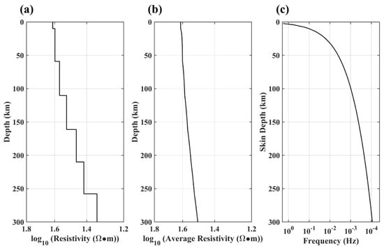
Figure 3.
(a) 1-D electrical resistivity mean model for mainland China []; (b) average resistivity at depth of h (km); and (c) relationship between skin depth and frequency.

Table 1.
The study frequency bands and corresponding depth.
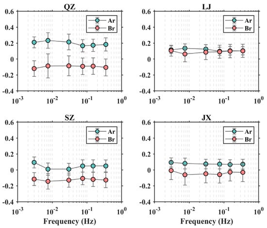
Figure 4.
Sounding curves for the four stations QZ, LJ, SZ, and JX. The displayed values are the median of all Ar, Br for the year 2019, and error bars represent 1 standard deviation of the population.
Figure 5 shows the results of the calculation process for obtaining PAmajor and PMmajor in the frequency band of 0.001–0.005 Hz at the QZ station in 2019. Figure 5a,c show the real parts of the coefficients of the magnetic transfer functions (Ar and Br). The thresholds (mean + 3σ, σ the standard deviation, black dashed lines in Figure 5a,c) of Ar and Br are 2.32 and 3.75, respectively. Figure 5b shows the distribution of PA in 0°–360° with a 10° interval, and they are mainly distributed at 120° (i.e., PAmajor, purple area). The radius denotes the counts of vectors in every azimuth bin. Figure 5d shows the distribution of all PM of obtained PAmajor, with the main distribution value of PM (i.e., 0.405, yellow dashed line in Figure 5d) as the PMmajor at the QZ station.
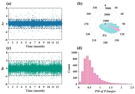
Figure 5.
The calculation process to obtain PAmajor and PMmajor. (a,c). The Ar, Br at the frequency band of 0.001–0.005 Hz at QZ station in 2019 respectively. The black dashed lines denote the thresholds; (b) the distribution of PA and the purple area denotes the PAmajor (120°), and the radius denotes the counts of vectors in every azimuth bin; and (d) the distribution of PM in PAmajor and the yellow dashed line is the major distribution of PM which represents the PMmajor.
Parkinson vectors composed of PAmajor and PMmajor at all stations were obtained at depths of 4–7 km, 7–10 km, 10–14 km, 14–30 km, 30–44 km, and 44–100 km, denoted by red arrows in Figure 6. In the western region (longitude 72°–92°E), the vectors roughly point east at a depth of 4–14 km (Figure 6a–c), whereas the vectors from one or two stations point in other directions at a depth of 14–100 km (Figure 6d–f), which may be due to the inhomogeneous conductivity structures there. In the center of mainland China (longitude 92°–108°E), there are mainly two regions where the PAmajor mostly points toward (or backward) at all study depths, which are indicated by the green (or blue) lines, respectively, in Figure 6a–f. Along the green lines (Figure 6a–f), the PAmajor on both sides points to here, while at the blue lines (Figure 6a–f), the PAmajor on both sides deviates from the region. This suggests that relatively high- or low-conductivity materials exist in these particular areas owing to the underlying inhomogeneous electrical materials. Note that the low-conductivity materials (blue lines) at two depth ranges of 30–45 km (Figure 6e) and 45–100 km (Figure 6f) are distributed northwest to those at the lower layers (Figure 6a–d). In the northern China (longitude 108°–120°E, latitude 32°–42°N), the vectors point to the areas of longitude 111°–113°E, latitude 35°–41°N at all study depths (i.e., green lines, Figure 6a–f), which indicates the highly conductive structures here. The vectors from stations in the western Bohai Sea point toward the sea, which may be owing to the geomagnetic coast effect at a depth of 4–14 km (Figure 6a–c), whereas at depths between 14 km and 100 km (Figure 6d–f), the vectors from several stations in the inland (southwest direction) area may be affected by highly conductive materials. In southwest mainland China, due to the geomagnetic coast effect, the vectors from the stations along the coast are directed toward the Yellow Sea, East China Sea, and South China Sea at all study depths (Figure 6a–f), which agrees with the observations by [,]. In the northeast of mainland China (longitude 115°–132°E, latitude 42°–52°N), the directions of vectors from three stations are almost the same at different study depths (Figure 6a–f). This indicates that high-conductivity materials near the stations in this area are distributed over a wide depth range. Nevertheless, we may obtain more information when more stations are established in this area in the future.
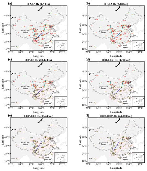
Figure 6.
The distribution of Parkinson vectors (red arrows) at the depth of 4–7 km (a); 7–10 km (b); 10–14 km (c); 14–30 km (d); 30–44 km (e); and 44–100 km (f), respectively, in mainland China. The black dots indicate the permanent geomagnetic stations. The green and blue lines indicate the electrical conductivity and resistivity region, respectively.
The Parkinson vectors point to conductors, and the backward of Parkinson vectors will point to the resistors []. The magnitude of the vector is inversely proportional to the distance from high-conductivity materials concluded from observed data and numerical modelling [,,], that the magnitude is larger when the vector is close to conductors or resistors. Due to that the three obvious electrical materials (i.e., green, and blue lines in Figure 6) indicated by Parkinson vectors are roughly in the north-south direction and to clarify quantitatively the distribution of these materials, we construct the maps of electrical conductivity structures by PMP, defined by Formula (7),
The 0 value areas of PMP in the maps indicate the conductors or resistors. The conductors are distributed in the areas where the left side values are positive and the right-side ones are negative. For resistors, the condition is reversed. The distributions of conductors and resistors are shown in Figure 7.
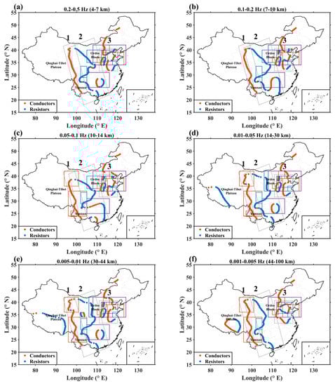
Figure 7.
The distribution of conductors (red areas) and resistors (blue areas) at the depth of 4–7 km (a); 7–10 km (b); 10–14 km (c); 14–30 km (d); 30–44 km (e); and 44–100 km (f), respectively, in mainland China. The dashed rectangles represent three main study areas. The triangles indicate the permanent magnetic stations. The squares are the study areas retrieved from the references in Discussion. The red and blue squares indicate the areas where scientists study the high-conductivity [,,,,,] and resistivity structures [,,,], respectively. The purple squares are the areas where both two electrical structures exist here [].
Figure 7a–f show the distribution of conductors and resistors in mainland China at depths of 4–7, 7–10, 10–14, 14–30, 30–44, and 44–100 km. We concentrated on the area of longitude 95°–120°E in this work because of the sparse station distribution in other regions (i.e., six stations in longitude 72°–95°E, three stations in latitude, 42°–52°N), and we divided the study area into main three parts from west to east, as shown in Figure 7. In part 1, a high-conductivity band at all study depth ranges (Figure 7a–f) exists, which is distributed along the east of the QTP and extends to the west of Yunnan. In part 2, overall high-resistivity bodies with some regional low-resistivity structures at all study depths (Figure 7a–f) exist, while at a depth between 44 km and 100 km (Figure 7f), the location of all electrical bodies is relatively west compared with the upper layers (Figure 7a–e). At the area of latitude 35°–40°N, the resistors at the depths of 4–14 km and 44–100 km (Figure 7a–c,f) are distributed at the longitudes 100°–108°E, which are nearly in the northwest-southeast direction, while the resistors at the depth of 14–45 km (Figure 7d,e) are located at longitude 108°E in north-south direction. At depths of 4–10 km (Figure 7a) and 14–44 km (Figure 7d,e), we note regional electrical bodies in the area of longitude 110°E, latitude 27°N. In Part 3, we note discontinuously distributed long conductors at an area of longitude 112–113°E, latitude 35°–45°N from 4 km to 100 km (Figure 7a–f). In the eastern neighboring of the conductors in this area, resistors exist at a depth of 4–44 km (Figure 7a–e). In the area of longitude 115–120°E, latitude 32°–38°N, the distribution of the electrical conductivity structures is almost the same at the depths between 4 km and 14 km (Figure 7a–c). In the 14–30 km (Figure 7d) and 30–44 km (Figure 7e) layers, a conductivity body is distributed at the same area of longitude 115°E, latitude 32°–38°N. At a depth of 44–100 km (Figure 7f), there are two resistivity bodies at longitudes 112–118°E and latitudes 34°–40°N.
3. Discussions
Herein, we compared the distribution of the underlying conductivity structures with results from previous studies utilizing the MT method. We retrieved the study areas of previous MT research in Figure 7 for better comparison. As for the long conductivity band in Part 1, previous MT studies have investigated the electrical conductivity structures in different regional areas in the eastern QTP [,] and western Yunnan [], and the corresponding depth ranges of high-conductivity structures are 10–100 km [,] and 10–30 km [], respectively. The long-conductivity band obtained in this study is distributed at a depth of 4–100 km (Figure 7a–f), which is consistent with the region in the eastern QTP at 10–100 km [,] (Figure 7c–f). Nevertheless, some discrepancies in depth exist in western Yunnan compared to Ye et al. [] (i.e., 10–30 km, Figure 7c,d). Meanwhile, distinct geophysical data [,,,,] were used to study the area in Part 1. Low-density anomalies at depths between 0 km and 250 km were revealed by the Earth Gravitational Model 2008 [] over the entire area of Part 1. Low-velocity (Vs.) anomalies were found at depths between 5 km and 100 km in the same area [,]. Combining the results of long high-conductivity bands in this study and previous multiple geophysical inversion results in the area of Part 1, the high-conductivity, low-density, and low-velocity materials may be large-scale (i.e., latitude 22°–40°N) plastic bodies []. This indicates that the crust and upper mantel here are easily deformed due to the collision of the Indian and Asian continents. This can provide an explanation for the large-scale surface motion in the eastern Qinghai-Tibet Plateau [].
For Part 2, the resistors from 35°N to 40°N had two types of distributions at different depths. One was toward the northwest-southeast direction (100°–107°E) at a depth of 4–14 km (Figure 7a–c), which is consistent with [,] (Figure 7a–c). The high-resistivity characteristic in this area was interpreted by the basalt distribution []. As in Li et al. [], the other resistors were approximately in the north-south direction (107°E) at a depth of 14–44 km (Figure 7d,e). This high-resistivity layer represents a rigid structure at the west edge of the Ordos Block []. The discrepancy in conductivity at different depths in this area is consistent with the results of [], indicating that conductivity significantly varied across the western edge of the Ordos block. As for the resistors at latitudes 30°–35°N, Zhao et al. [] studied the electrical conductivity structures via the MT method using three profiles in this area, and found that high-resistivity bodies were distributed at depths between 0 km and 60 km, which almost coincide with our results at depths of 4–44 km (Figure 7a–e). In the deep layer of 44–100 km (Figure 7f), the high-resistivity bodies extended to the west compared to the shallow layers (Figure 7a–e); this phenomenon can be found in the MT profile by [] (Figure 7a–f). The high-resistivity bodies in the shallow layers (Figure 7a–e) are referred to as the Pengguan Massif [], a region of Proterozoic crystal-line rocks exposed in this area [], and the deep resistors in Figure 7f may be associated with basement rocks []. In the case of the areas at latitude 20°–30°N in part 2, we noted distributed resistive bulks with regional conductors between them at 4–44 km (Figure 7a–e). In contrast, compared with the upper layers, the distribution of electrical bodies below 44 km (Figure 7f) was concentrated relatively west (Figure 7a–e). The spatial distribution of the electrical conductivity structures in this area is roughly consistent with the results of [] (Figure 7a–e). Resistive bodies indicate the basic features of a stable Precambrian tectonic setting [] (Figure 7a–e). In summary, the areas of Part 2 are mainly resistive, which suggests that the structures are overall rigid [,,] in central mainland China. This indicates that stress is easily accumulated here and causes the region of strong seismic activity.
In Section 3, we compared the results of this study with those of previous studies [,,,,,]. The conductors in this area are consistent with the results of the MT sounding [,,,] (Figure 7a–f). Conversely, the resistors roughly correspond with the results of [,] (Figure 7a–f). In general, there are high-low-high-low conductive structures from west to east at a depth of 4–100 km (Figure 7a–f), which is consistent with [] (Figure 7a–f), who investigated the electrical resistivity structures of the lithosphere beneath the entirety of North China (longitude 104°–125°E, latitude 35°–41°E) based on 1° (latitude) × 1° (longitude) standard MT array. The tectonic evolution of the North China Craton has been fully studied using geology, geochemistry, and geochronology [,]. The North China Craton is usually divided into three blocks: Western Blocks, Trans-North China Orogen, and Eastern Blocks []. Part 3 of this work was located in the North China Craton, and the distribution of the separated electrical bodies from west to east in this region provides geophysical evidence that the Craton is composed of multiple blocks.
Above all, we are confident of the locations of the electrical conductivity structures in this work by comparing them with those of previous studies using the MT method in mainland China. The results of two methods are consistent. This suggests that utilizing Parkinson vectors derived from permanent geomagnetic stations to map conductors and/or resistors is an effective alternative method for investigating the distribution of underlying conductivity structures.
4. Conclusions
In this study, we obtained the distribution of the underlying electrical conductivity structures in mainland China using Parkinson vectors through a magnetic transfer function utilizing permanent geomagnetic data. Generally, the Parkinson vectors in the west of China point to the eastern QTP. In central mainland China, the vectors deviate in this region. As for the northeast of China, the distribution of vectors is complicated, which reflect the complex tectonic activity here. The geomagnetic coast effect is clear at the southeast coast of China. We found a high-conductivity band distributed along the east of the QTP and extending to the west of Yunnan at depths of 4–100 km. Overall high-resistivity bodies at depths of 4–100 km with some regional high-conductivity structures at 4–44 km exist in central China. In addition, the separated high- and low-conductivity electrical bodies are distributed in the northeast of China.
Our results are highly consistent with the electrical resistivity structures obtained by the MT method, thereby indicating the reliability of our method. We divided the results into three parts and found that large-scale plastic high-conductivity bodies exist east of the QTP and west of Yunnan. This can provide an explanation for the large-scale surface motion in the eastern Qinghai-Tibet Plateau. In central mainland China, the highly resistive indicates overall rigid structures, which indicates that stress is easily accumulated here, and causes the region of strong seismic activity. The separated high-and low-conductivity electrical bodies in the North China Craton provide geophysical evidence that the Craton is composed of multiple blocks. The distribution of the underlying electrical conductivity structures in this work can provide an overall perspective for the study of tectonic evolution and geodynamics in mainland China.
Author Contributions
Conceptualization, Z.M. and C.-H.C.; methodology, Z.M.; software, Z.M.; validation, Z.M. and C.-H.C.; formal analysis, Z.M.; investigation, A.Y.; resources, A.Y.; data curation, A.Y.; writing—original draft preparation, Z.M.; writing—review and editing, C.-H.C., B.C., J.Y., Y.G., Y.-Y.S. and K.L.; visualization, Z.M.; supervision, C.-H.C.; project administration, Z.M.; funding acquisition, C.-H.C. and A.Y. All authors have read and agreed to the published version of the manuscript.
Funding
This research was funded by the Joint Funds of the National Natural Science Foundation of China, grant number U2039205; the Special Training Project of National Science Foundation of Xinjiang Uygur Autonomous Region, grant number 2022D03031, Seismic Regime Tracking Project of CEA, grant number 2023010415, and The APC was funded by U2039205.
Data Availability Statement
The data utilized in this study can be downloaded at https://doi.org/10.5281/zenodo.5917804, accessed on 27 Feburary 2023.
Acknowledgments
The authors acknowledge the Geomagnetic Network Center of China, Institute of Geophysics, China Earthquake Administration for providing geomagnetic data for this study. The authors are immensely grateful to the Editor and reviewers for their valuable comments on our manuscript.
Conflicts of Interest
The authors declare no conflict of interest.
References
- Gao, J.; Zhang, H.; Zhang, S.; Xin, H.; Li, Z.; Tian, W.; Bao, F.; Cheng, Z.; Jia, X.; Fu, L. Magma recharging beneath the Weishan volcano of the intraplate Wudalianchi volcanic field, northeast China, implied from 3-D magnetotelluric imaging. Geology 2020, 48, 913–918. [Google Scholar] [CrossRef]
- Han, Q.; Kelbert, A.; Hu, X. An electrical conductivity model of a coastal geothermal field in southeastern China based on 3D magnetotelluric imaging. Geophysics 2021, 86, B265–B276. [Google Scholar] [CrossRef]
- Kang, M.; Xin, H.-l.; Kang, J.; Xiong, W. Crustal Structure and Seismogenic Background Beneath Zhumadian, Henan, China: Evidence from Magnetotelluric Data. Pure Appl. Geophys. 2021, 178, 1643–1659. [Google Scholar] [CrossRef]
- Tang, Y.; Weng, A.; Yang, Y.; Li, S.; Niu, J.; Zhang, Y.; Li, Y.; Li, J. Connection between earthquakes and deep fluids revealed by magnetotelluric imaging in Songyuan, China. Sci. China Earth Sci. 2021, 64, 161–176. [Google Scholar] [CrossRef]
- Wei, W.; Jin, S.; Ye, G.; Deng, M.; Jing, J.; Unsworth, M.; Jones, A.G. Conductivity structure and rheological property of lithosphere in Southern Tibet inferred from super-broadband magnetotelluric sounding. Sci. China Earth Sci. 2010, 53, 189–202. [Google Scholar] [CrossRef]
- Wu, C.; Hu, X.; Wang, G.; Xi, Y.; Lin, W.; Liu, S.; Yang, B.; Cai, J. Magnetotelluric imaging of the Zhangzhou Basin geothermal zone, Southeastern China. Energies 2018, 11, 2170. [Google Scholar] [CrossRef]
- Xiao, Q.; Shao, G.; Liu-Zeng, J.; Oskin, M.E.; Zhang, J.; Zhao, G.; Wang, J. Eastern termination of the Altyn Tagh Fault, western China: Constraints from a magnetotelluric survey. J. Geophys. Res. Solid Earth 2015, 120, 2838–2858. [Google Scholar] [CrossRef]
- Xiao, Q.; Zhang, J.; Zhao, G.; Wang, J. Electrical resistivity structures northeast of the Eastern Kunlun Fault in the Northeastern Tibet: Tectonic implications. Tectonophysics 2013, 601, 125–138. [Google Scholar] [CrossRef]
- Xu, Y.; Yang, B.; Zhang, A.; Wu, S.; Zhu, L.; Yang, Y.; Wang, Q.; Xia, Q. Magnetotelluric imaging of a fossil oceanic plate in northwestern Xinjiang, China. Geology 2020, 48, 385–389. [Google Scholar] [CrossRef]
- Ye, T.; Chen, X.; Huang, Q.; Zhao, L.; Zhang, Y.; Uyeshima, M. Bifurcated crustal channel flow and seismogenic structures of intraplate earthquakes in Western Yunnan, China as revealed by three-dimensional magnetotelluric imaging. J. Geophys. Res. Solid Earth 2020, 125, e2019JB018991. [Google Scholar] [CrossRef]
- Zhang, H.; Huang, Q.; Zhao, G.; Guo, Z.; Chen, Y.J. Three-dimensional conductivity model of crust and uppermost mantle at the northern Trans North China Orogen: Evidence for a mantle source of Datong volcanoes. Earth Planet. Sci. Lett. 2016, 453, 182–192. [Google Scholar] [CrossRef]
- Zhang, L.; Jin, S.; Wei, W.; Ye, G.; Jing, J.; Dong, H.; Xie, C. Lithospheric electrical structure of South China imaged by magnetotelluric data and its tectonic implications. J. Asian Earth Sci. 2015, 98, 178–187. [Google Scholar] [CrossRef]
- Zhang, L.; Zhao, C.; Yu, P.; Xiang, Y.; Peng, X.; Koyama, T.; Yang, W. The electrical conductivity structure of the Tarim basin in NW China as revealed by three-dimensional magnetotelluric inversion. J. Asian Earth Sci. 2020, 187, 104093. [Google Scholar] [CrossRef]
- Zhang, P.; Fang, H.; Zhong, Q.; Zhang, X.; Yuan, Y.; Liu, J. Structural features and tectonic evolution of the Nenjiang–Balihan fault in the western margin of the Songliao Basin, NE China, inferred from 2D inversion of magnetotelluric data. J. Asian Earth Sci. 2021, 206, 104628. [Google Scholar] [CrossRef]
- Bai, D.; Unsworth, M.J.; Meju, M.A.; Ma, X.; Teng, J.; Kong, X.; Sun, Y.; Sun, J.; Wang, L.; Jiang, C. Crustal deformation of the eastern Tibetan plateau revealed by magnetotelluric imaging. Nat. Geosci. 2010, 3, 358–362. [Google Scholar] [CrossRef]
- Zhao, G.; Unsworth, M.J.; Zhan, Y.; Wang, L.; Chen, X.; Jones, A.G.; Tang, J.; Xiao, Q.; Wang, J.; Cai, J. Crustal structure and rheology of the Longmenshan and Wenchuan Mw 7.9 earthquake epicentral area from magnetotelluric data. Geology 2012, 40, 1139–1142. [Google Scholar] [CrossRef]
- Li, X.; Bai, D.; Ma, X.; Chen, Y.; Varentsov, I.M.; Xue, G.; Xue, S.; Lozovsky, I. Electrical resistivity structure of the Xiaojiang strike-slip fault system (SW China) and its tectonic implications. J. Asian Earth Sci. 2019, 176, 57–67. [Google Scholar] [CrossRef]
- Hu, X.; Lin, W.; Yang, W.; Yang, B. A review on developments in the electrical structure of craton lithosphere. Sci. China Earth Sci. 2020, 63, 1661–1677. [Google Scholar] [CrossRef]
- Wei, W.; Ye, G.; Jin, S.; Deng, M.; Jing, J.; Peng, Z.; Lin, X.; Song, S.; Tang, B.; Qu, S.; et al. Geoelectric structure of lithosphere beneath Eastern North China: Features of thinned lithosphere from magnetotelluric soundings. Earth Sci. Front. 2008, 15, 204–216. [Google Scholar] [CrossRef]
- Xiao, Q.; Zhao, G.; Wang, J.; Zhan, Y.; Chen, X.; Tang, J.; Cai, J.; Wan, Z.; Wang, L.; Ma, W. Deep electrical structure of the Sulu orogen and neighboring areas. Sci. China Ser. D Earth Sci. 2009, 52, 420–430. [Google Scholar] [CrossRef]
- Ye, G.; Liu, C.; Luo, X.; Jin, S.; Wei, W.; Dong, H.; Yin, Y. Dynamical significance of the Tanlu Fault Zone in the destruction of the North China Craton: The evidence provided by the three-dimensional Magnetotelluric array study. Tectonophysics 2021, 813, 228910. [Google Scholar] [CrossRef]
- Yin, Y.; Jin, S.; Wei, W.; Santosh, M.; Dong, H.; Xie, C. Construction and destruction of the North China Craton with implications for metallogeny: Magnetotelluric evidence from the Hengshan–Wutai–Fuping region within Trans-North China Orogen. Gondwana Res. 2016, 40, 21–42. [Google Scholar] [CrossRef]
- Dong, H.; Wei, W.; Ye, G.; Jin, S.; Jones, A.G.; Jing, J.; Zhang, L.; Xie, C.; Zhang, F.; Wang, H. Three-dimensional electrical structure of the crust and upper mantle in Ordos Block and adjacent area: Evidence of regional lithospheric modification. Geochem. Geophys. Geosyst. 2014, 15, 2414–2425. [Google Scholar] [CrossRef]
- Yuan, Y.; Uyeshima, M.; Huang, Q.; Tang, J.; Li, Q.; Teng, Y. Continental-scale deep electrical resistivity structure beneath China. Tectonophysics 2020, 790, 228559. [Google Scholar] [CrossRef]
- Siripunvaraporn, W. Three-dimensional magnetotelluric inversion: An introductory guide for developers and users. Surv. Geophys. 2012, 33, 5–27. [Google Scholar] [CrossRef]
- Chen, C.-H.; Sun, Y.-Y.; Lin, K.; Zhou, C.; Xu, R.; Qing, H.; Gao, Y.; Chen, T.; Wang, F.; Yu, H. A new instrumental array in Sichuan, China, to monitor vibrations and perturbations of the lithosphere, atmosphere, and ionosphere. Surv. Geophys. 2021, 42, 1425–1442. [Google Scholar] [CrossRef]
- Smith, Z.; Murtagh, W.; Smithtro, C. Relationship between solar wind low-energy energetic ion enhancements and large geomagnetic storms. J. Geophys. Res. Space Phys. 2004, 109. [Google Scholar] [CrossRef]
- Vassiliadis, D.; Sharma, A.; Eastman, T.; Papadopoulos, K. Low-dimensional chaos in magnetospheric activity from AE time series. Geophys. Res. Lett. 1990, 17, 1841–1844. [Google Scholar] [CrossRef]
- Wen, S.; Chen, C.H.; Yen, H.Y.; Yeh, T.K.; Liu, J.Y.; Hattori, K.; Han, P.; Wang, C.H.; Shin, T.C. Magnetic storm free ULF analysis in relation with earthquakes in Taiwan. Nat. Hazards Earth Syst. Sci. 2012, 12, 1747–1754. [Google Scholar] [CrossRef]
- Chen, C.H.; Lin, J.Y.; Gao, Y.; Lin, C.H.; Han, P.; Chen, C.R.; Lin, L.C.; Huang, R.; Liu, J.Y. Magnetic pulsations triggered by microseismic ground motion. J. Geophys. Res. Solid Earth 2021, 126, e2020JB021416. [Google Scholar] [CrossRef]
- Gao, Y.; Harris, J.M.; Wen, J.; Huang, Y.; Twardzik, C.; Chen, X.; Hu, H. Modeling of the coseismic electromagnetic fields observed during the 2004 Mw 6.0 Parkfield earthquake. Geophys. Res. Lett. 2016, 43, 620–627. [Google Scholar] [CrossRef]
- Chen, C.-H.; Sun, Y.-Y.; Zhang, X.; Wang, F.; Lin, K.; Gao, Y.; Tang, C.-C.; Lyu, J.; Huang, R.; Huang, Q. Far-field coupling and interactions in multiple geospheres after the Tonga volcano eruptions. Surv. Geophys. 2022, 19, 1–5. [Google Scholar] [CrossRef]
- Mao, Z.; Chen, C.-H.; Zhang, S.; Yisimayili, A.; Yu, H.; Yu, C.; Liu, J.-Y. Locating Seismo-Conductivity Anomaly before the 2017 MW 6.5 Jiuzhaigou Earthquake in China Using Far Magnetic Stations. Remote Sens. 2020, 12, 1777. [Google Scholar] [CrossRef]
- Chen, C.H.; Hsu, H.L.; Wen, S.; Yeh, T.K.; Chang, F.Y.; Wang, C.H.; Liu, J.Y.; Sun, Y.Y.; Hattori, K.; Yen, H.Y.; et al. Evaluation of seismo-electric anomalies using magnetic data in Taiwan. Nat. Hazards Earth Syst. Sci. 2013, 13, 597–604. [Google Scholar] [CrossRef]
- Chen, C.H.; Lin, C.H.; Wang, C.H.; Liu, J.Y.; Yeh, T.K.; Yen, H.Y.; Lin, T.W. Potential relationships between seismo-deformation and seismo-conductivity anomalies. J. Asian Earth Sci. 2015, 114, 327–337. [Google Scholar] [CrossRef]
- Parkinson, W. Directions of rapid geomagnetic fluctuations. Geophys. J. Int. 1959, 2, 1–14. [Google Scholar] [CrossRef]
- Parkinson, W. The influence of continents and oceans on geomagnetic variations. Geophys. J. Int. 1962, 6, 441–449. [Google Scholar] [CrossRef]
- Schmucker, U. Regional induction studies: A review of methods and results. Phys. Earth Planet. Inter. 1973, 7, 365–378. [Google Scholar] [CrossRef]
- Parkinson, W.; Jones, F. The geomagnetic coast effect. Rev. Geophys. 1979, 17, 1999–2015. [Google Scholar] [CrossRef]
- Edwards, R.; Greenhouse, J. Geomagnetic variations in the eastern United States: Evidence for a highly conducting lower crust? Science 1975, 188, 726–728. [Google Scholar] [CrossRef]
- Gong, S.; Liu, S.; Liang, M. Characteristics of geomagnetic Parkinson vector in Chinese mainland and their tectonic implication. Acta Seismol. Sin. 2017, 39, 47–63. [Google Scholar] [CrossRef]
- Niblett, E.; DeLaurier, J.; Law, L.; Plet, F. Geomagnetic variation anomalies in the Canadian Arctic I. Ellesmere Island and Lincoln Sea. J. Geomagn. Geoelectr. 1974, 26, 203–221. [Google Scholar] [CrossRef]
- Schmucker, U. Anomalies of geomagnetic variations in the southwestern United States. J. Geomagn. Geoelectr. 1964, 15, 193–221. [Google Scholar] [CrossRef]
- White, A.; Polatajko, O. The coast effect in geomagnetic variations in South Australia. J. Geomagn. Geoelectr. 1978, 30, 109–120. [Google Scholar] [CrossRef]
- Favetto, A.; Pomposiello, C.; de Luchi, M.G.L.; Booker, J. 2D Magnetotelluric interpretation of the crust electrical resistivity across the Pampean terrane–Río de la Plata suture, in central Argentina. Tectonophysics 2008, 459, 54–65. [Google Scholar] [CrossRef]
- Wang, C.-Y.; Sandvol, E.; Zhu, L.; Lou, H.; Yao, Z.; Luo, X. Lateral variation of crustal structure in the Ordos block and surrounding regions, North China, and its tectonic implications. Earth Planet. Sci. Lett. 2014, 387, 198–211. [Google Scholar] [CrossRef]
- Zhang, S.; Xu, Y.; Jiang, L.; Yang, B.; Liu, Y.; Griffin, W.; Luo, Y.; Huang, R.; Zhou, Y.; Zhang, L. Electrical structures in the northwest margin of the Junggar basin: Implications for its late Paleozoic geodynamics. Tectonophysics 2017, 717, 473–483. [Google Scholar] [CrossRef]
- Araya Vargas, J.; Ritter, O. Source effects in mid-latitude geomagnetic transfer functions. Geophys. J. Int. 2016, 204, 606–630. [Google Scholar] [CrossRef]
- Rokityansky, I.; Klymkovych, T.; Babak, V.; Isac, A. Annual and diurnal variations of induction vectors in relation to geodynamic processes. Geomat. Nat. Hazards Risk 2012, 3, 239–249. [Google Scholar] [CrossRef]
- Simpson, F.; Bahr, K. Practical Magnetotellurics; Cambridge University Press: Cambridge, UK, 2005. [Google Scholar] [CrossRef]
- Yuan, Y.; Huang, Q.; Li, Q.; Teng, Y. Geomagnetic vertical transfer function revealed from multi-interval geomagnetic data. Earthq. Sci. 2019, 32, 229–234. [Google Scholar] [CrossRef]
- DeLaurier, J.M.; Auld, D.; Law, L. The Geomagnetic Response Across the Continental Margin off Vancouver Island Comparison of Results from Numerical Modelling and Field Data. J. Geomagn. Geoelectr. 1983, 35, 517–528. [Google Scholar] [CrossRef]
- Bao, X.; Sun, X.; Xu, M.; Eaton, D.W.; Song, X.; Wang, L.; Ding, Z.; Mi, N.; Li, H.; Yu, D. Two crustal low-velocity channels beneath SE Tibet revealed by joint inversion of Rayleigh wave dispersion and receiver functions. Earth Planet. Sci. Lett. 2015, 415, 16–24. [Google Scholar] [CrossRef]
- Chen, H.; Zhu, L.; Su, Y. Low velocity crustal flow and crust–mantle coupling mechanism in Yunnan, SE Tibet, revealed by 3D S-wave velocity and azimuthal anisotropy. Tectonophysics 2016, 685, 8–20. [Google Scholar] [CrossRef]
- Dong, X.; Yang, D.; Zhu, H. Adjoint Tomography of the Lithospheric Structure beneath Northeastern Tibet. Seismol. Soc. Am. 2020, 91, 3304–3312. [Google Scholar] [CrossRef]
- Li, H.; Fang, J. Crustal and upper mantle density structure beneath the Qinghai-Tibet plateau and surrounding areas derived from EGM2008 geoid anomalies. ISPRS Int. J. Geo-Inf. 2017, 6, 4. [Google Scholar] [CrossRef]
- Li, M.; Zhang, S.; Wang, F.; Wu, T.; Qin, W. Crustal and upper-mantle structure of the southeastern Tibetan Plateau from joint analysis of surface wave dispersion and receiver functions. J. Asian Earth Sci. 2016, 117, 52–63. [Google Scholar] [CrossRef]
- Wang, M.; Shen, Z.K. Present-day crustal deformation of continental China derived from GPS and its tectonic implications. J. Geophys. Res. Solid Earth 2020, 125, e2019JB018774. [Google Scholar] [CrossRef]
- Xin, Z.; Han, J.; Gao, R.; Guo, X.; Liang, H.; Kang, J.; Liu, L. Electrical structure of the eastern segment of the Qilian orogenic belt revealed by 3-D inversion of magnetotelluric data: New insights into the evolution of the northeastern margin of the Qinghai-Tibet Plateau. J. Asian Earth Sci. 2021, 210, 104707. [Google Scholar] [CrossRef]
- LI, C.-J.; BAI, D.-H.; XUE, S.; LI, X.; MA, X.-B.; YAN, Y.-L.; KONG, X.-R. A magnetotelluric study of the deep electric structure beneath the Ordos Block. Chin. J. Geophys. 2017, 60, 1788–1799. [Google Scholar] [CrossRef]
- Xu, X.; Wen, X.; Yu, G.; Chen, G.; Klinger, Y.; Hubbard, J.; Shaw, J. Coseismic reverse-and oblique-slip surface faulting generated by the 2008 Mw 7.9 Wenchuan earthquake, China. Geology 2009, 37, 515–518. [Google Scholar] [CrossRef]
- Gürer, A.; Bayrak, M. Relation between electrical resistivity and earthquake generation in the crust of West Anatolia, Turkey. Tectonophysics 2007, 445, 49–65. [Google Scholar] [CrossRef]
- Yin, Y.; Jin, S.; Wei, W.; Ye, G.; Zhang, L.; Dong, H.; Xie, C.; Liang, H. Lithospheric rheological heterogeneity across an intraplate rift basin (Linfen Basin, North China) constrained from magnetotelluric data: Implications for seismicity and rift evolution. Tectonophysics 2017, 717, 1–15. [Google Scholar] [CrossRef]
- Wei, W.; Ye, G.; Jin, S.; Jing, J.; Ji, L.; Dong, H.; Zhang, L.; Yin, Y.; Xie, C. Experiments of magnetotelluric observation network on North China and lithospheric conductivity structure from fast imaging method. Chin. J. Geophys. 2018, 61, 2508–2524. [Google Scholar] [CrossRef]
- Kusky, T.M.; Li, J. Paleoproterozoic tectonic evolution of the North China Craton. J. Asian Earth Sci. 2003, 22, 383–397. [Google Scholar] [CrossRef]
- Zhao, G.; Wilde, S.A.; Cawood, P.A.; Sun, M. Archean blocks and their boundaries in the North China Craton: Lithological, geochemical, structural and P–T path constraints and tectonic evolution. Precambrian Res. 2001, 107, 45–73. [Google Scholar] [CrossRef]
Disclaimer/Publisher’s Note: The statements, opinions and data contained in all publications are solely those of the individual author(s) and contributor(s) and not of MDPI and/or the editor(s). MDPI and/or the editor(s) disclaim responsibility for any injury to people or property resulting from any ideas, methods, instructions or products referred to in the content. |
© 2023 by the authors. Licensee MDPI, Basel, Switzerland. This article is an open access article distributed under the terms and conditions of the Creative Commons Attribution (CC BY) license (https://creativecommons.org/licenses/by/4.0/).