Bivariate Landslide Susceptibility Analysis: Clarification, Optimization, Open Software, and Preliminary Comparison

Abstract

Bivariate data-driven methods have been widely used in landslide susceptibility analysis. However, the names, principles, and correlations of bivariate methods are still confused. In this paper, the names, principles, and correlations of bivariate methods are first clarified based on a comprehensive and in-depth survey. A total of eleven prevalent bivariate methods are identified, nominated, and elaborated in a general framework, constituting a well-structured bivariate method family. We show that all prevalent bivariate methods depend on empirical conditional probabilities of landslide occurrence to calculate landslide susceptibilities, either exclusively or inclusively. It is clarified that those eight “conditional-probability-based” bivariate methods, which exclusively depend on empirical conditional probabilities, are particularly strongly correlated in principle, and therefore are expected to have a very close or even the same performance. It is also suggested that conditional-probability-based bivariate methods apply to a “classification-free” modification, in which factor classifications are avoided and the result is dominated by a single parameter, “bin width”. Then, a general optimization framework for conditional-probability-based bivariate methods, based on the classification-free modification and obtaining optimum results by optimizing the dominant parameter bin width, is proposed. The open software Automatic Landslide Susceptibility Analysis (ALSA) is updated to implement the eight conditional-probability-based bivariate methods and the general optimization framework. Finally, a case study is presented, which confirms the theoretical expectation that different conditional-probability-based bivariate methods have a very close or even the same performance, and shows that optimal bivariate methods perform better than conventional bivariate methods regarding both the prediction rate and the ability to reveal the quasi-continuous varying pattern of sensibilities to landslides for individual predisposing factors. The principles and open software presented in this study provide both theoretical and practical foundations for applications and explorations of bivariate methods in landslide susceptibility analysis.

1. Introduction

Landslide susceptibility is an assessment of the relative spatial probability of landslides, and, more comprehensively, should include an assessment of landslide type and size whenever possible [1,2]. Landslide susceptibility discussed in this paper only estimates where landslides are likely to occur, as in most other studies [3]. The methods of landslide susceptibility analysis can be grouped into three fundamental categories, namely, qualitative “knowledge-driven” methods, quantitative “data-driven” methods, and quantitative “physically based” methods [4]. Data-driven methods use data from past landslide occurrences to quantitatively evaluate the relative sensibilities of the predisposing conditions to slope failures and have become standard in regional-scale landslide susceptibility assessment [4]. Data-driven methods broadly include bivariate methods and multivariate methods [5].

Bivariate data-driven methods, or simply bivariate methods, quantify sensibilities to landslides by assigning a favorability value for each class of individual predisposing factors [6]. The assignment of favorability values for an individual predisposing factor and the possible weighting of this factor only need two “variates”, i.e., the past landslide layer and the targeted classified factor layer, leading to the attributive “bivariate”. Favorability layers for all the considered predisposing factors are combined based on certain combination rules to finally obtain a landslide susceptibility index (LSI) layer. Although bivariate methods have some intrinsic disadvantages, for example, difficulties in considering dependencies between and relative weights of individual predisposing factors, they have been and are still commonly used in landslide susceptibility analysis. The ongoing wide application of bivariate methods is due to, on the one hand, the simplicity of the principles behind them, and on the other hand, their ability to reveal the sensibilities of different factor values to slope failures for individual predisposing factors [5,7].

Many bivariate methods have been proposed and applied in landslide susceptibility analysis. However, the wide application of various bivariate methods has also introduced widespread confusion. First, the names of bivariate methods are confused. There are dozens of names used to indicate bivariate methods (see Section 2.1). The confusion around names includes the facts that an identical bivariate method may have several names, and worse, an identical name may indicate different bivariate methods. In addition, some names used are not relevant enough to reflect the principles of bivariate methods. Second, the principles of bivariate methods are confused. For the same method, different authors may describe its principle in varied ways, causing difficulties in understanding and sometimes inconsistencies. More importantly, principles of different bivariate methods have never been elaborated in a general framework, making it impractical to reveal and define correlations between bivariate methods. Third, correlations between bivariate methods are confused. Although some bivariate methods are expected to be strongly correlated, there have been no theoretical investigations of correlations between bivariate methods. Correlations between bivariate methods have been practically ignored, making it difficult to make comparisons and choices between different methods. There are some literature reviews on methods of landslide susceptibility analysis [3,8,9,10]; however, names, principles, and correlations of bivariate methods still have not been systematically clarified yet. Therefore, the foremost aim of this paper is to clarify bivariate methods of landslide susceptibility analysis, making clear their names, principles, and correlations.

The classification of predisposing factors with continuous factor values is conventionally required in the first place by bivariate methods, which will induce a discontinuity problem and a subjectivity problem [5]. The discontinuity problem means that all factor values in the same class will have the same favorability value, eventually resulting in a discontinuity in the spatial distribution of landslide susceptibility. The subjectivity problem means that the choices of the number and divisions of factor classes are subjective, although it can be moderated by adopting a data-dependent classification [11]. To address the two problems associated with factor classifications, Li et al. proposed a new “classification-free” frequency ratio method [5], in which the classification of factors with continuous factor values is avoided, and an essential parameter “bin width” ranging from 0 to 1 dominates the derived landslide susceptibility result. The dominance of a single parameter further allows the optimization of landslide susceptibility assessment [12], which is achieved by finding an optimal bin width that yields a maximum AUC (area under the receiver operating characteristic (ROC) curve). The classification-free and, thus, the optimized frequency ratio method, have also shown better performances than the conventional frequency ratio method [5,12]. Since all (conventional) bivariate methods require factor classifications, it is tempting to apply the classification-free modification and further optimization to other applicable bivariate methods besides the frequency ratio method. The clarification of bivariate methods, which is the foremost aim of this paper, will also be the foundation for identifying those methods applicable to the classification-free modification and further allow a general application of the modification and optimization.

In this paper, bivariate methods of landslide susceptibility analysis are first clarified. Principles and correlations of those bivariate methods applicable to the classification-free modification are particularly clarified. Then, a general optimization framework for those bivariate methods applicable to the classification-free modification is presented, followed by an update of open software that implements the modification and the optimization framework. Finally, a preliminary comparison between different bivariate methods in both conventional and optimal scenarios is presented.

2. Clarification

This paper progressively clarifies the names, principles, and correlations of bivariate methods of landslide susceptibility analysis. This paper is not an inclusive review paper and thus will only cite a tiny part of the huge pool of publications relevant to the bivariate analysis of landslide susceptibility; some cited publications in this paper are only examples of those conveying similar content. Readers are referred to relevant review papers [3,8,9,10] for a comprehensive bibliography. Nevertheless, as far as we know, this is the first summarization of bivariate methods within a general framework (Figure 1;

Table 1. Summary of conditional-probability-based bivariate methods of landslide susceptibility analysis.

Method	Conditional Probabilities	Favorability Function	Combination Rule	Reference
Frequency contrast	p(L|Fi), p(L|Fi,j)	$p\left(L|F_{i,j}\right)-p\left(L|F_i\right)$	Direct summation	e.g., [14] in 1993
Frequency ratio	p(L|Fi), p(L|Fi,j)	$\frac{p\left(L|F_{i,j}\right)}{p\left(L|F_i\right)}$	Direct summation	e.g., [5] in 2017
Information value	p(L|Fi), p(L|Fi,j)	$\ln \left[\frac{p\left(L|F_{i,j}\right)}{p\left(L|F_i\right)}\right]$	Direct summation	e.g., [14] in 1993
Certainty factor	p(L|Fi), p(L|Fi,j)	$\{\begin{array}{c}\frac{p\left(L|F_{i,j}\right)-p\left(L|F_i\right)}{p\left(L|F_{i,j}\right)·\left[1-p\left(L|F_i\right)\right]}, p\left(L|F_{i,j}\right)\ge p\left(L|F_i\right)\\ \frac{p\left(L|F_{i,j}\right)-p\left(L|F_i\right)}{p\left(L|F_i\right)·\left[1-p\left(L|F_{i,j}\right)\right]}, p\left(L|F_{i,j}\right)<p\left(L|F_i\right)\end{array}$	Combination rule of certainty factor	e.g., [18] in 2004
Cosine amplitude	p(L|Fi,j), p(Fi,j|L)	$\sqrt{p\left(L|F_{i,j}\right)·p\left(F_{i,j}|L\right)}$	Direct summation	e.g., [19] in 2006
Weight of evidence	p(Fi,j|L), p(Fi,j|$\overline{L}$), p($\overline{F_{i,j}}$|L), p($\overline{F_{i,j}}$|$\overline{L}$)	$\ln \left[\frac{p\left(F_{i,j}|L\right)}{p\left(F_{i,j}|\overline{L}\right)}\right]-\ln \left[\frac{p\left(\overline{F_{i,j}}|L\right)}{p\left(\overline{F_{i,j}}|\overline{L}\right)}\right]+{\displaystyle \sum }_{k=1}^m\ln \left[\frac{p\left(\overline{F_{i,k}}|L\right)}{p\left(\overline{F_{i,k}}|\overline{L}\right)}\right]$	Direct summation, logit transformation	e.g., [28] in 1989
Weight contrast	p(Fi,j|L), p(Fi,j|$\overline{L}$), p($\overline{F_{i,j}}$|L), p($\overline{F_{i,j}}$|$\overline{L}$)	$\ln \left[\frac{p\left(F_{i,j}|L\right)}{p\left(F_{i,j}|\overline{L}\right)}\right]-\ln \left[\frac{p\left(\overline{F_{i,j}}|L\right)}{p\left(\overline{F_{i,j}}|\overline{L}\right)}\right]$	Direct summation	e.g., [29] in 2010
Sufficiency ratio	p(Fi,j|L), p(Fi,j|$\overline{L}$)	$\frac{p\left(F_{i,j}|L\right)}{p\left(F_{i,j}|\overline{L}\right)}$	Direct summation	e.g., [30] in 2001

Note: Details of conditional probabilities and favorability functions are referred to in the main text (Section 2.2).

). After clarification, the bivariate method family changes from an unstructured to a well-structured one (Figure 1).

2.1. Clarification of Names

To the best knowledge of the authors, currently, there are sixteen widely used names of bivariate methods (Figure 1a), including “frequency ratio” [5], “likelihood ratio” [13], “information value” [14], “landslide index” [15], “statistical index” [16], “relative effect” [17], “certainty factor” [18], “cosine amplitude” [19], “weight of evidence” [20], “index of entropy” [21], “entropy index” [22], “Dempster–Shafer” [23], “belief function” [24], “fuzzy logic” [25], “fuzzy set” [26], and “fuzzy approach” [27]. As mentioned in the Introduction, various uses of names have caused widespread confusion. It is therefore needed to appoint names for bivariate methods so that each method is assigned a name that is as recognized and relevant as possible, and one name indicates only one method.

We identified a total of eleven prevalent bivariate methods of landslide susceptibility analysis based on a comprehensive survey of relevant publications (Figure 1b), and we named them the “frequency contrast” method [14], the “frequency ratio” method [5], the “information value” method [14], the “certainty factor” method [18], the “cosine amplitude” method [19], the “weight of evidence” method [28], the “weight contrast” method [29], the “sufficiency ratio” method [30], the “index of entropy” method [22], the “Dempster–Shafer” method [24], and the “fuzzy logic” method [25]. The following strategies have been adopted to appoint names.

(1)

If several names indicate an identical method, we used the most recognized one. For example, “information value” [14], “landslide index” [15], “statistical index” [16], and “relative effect” [17] indicate the same method, and among them, “information value” is the most recognized one (Figure 1a). Similarly, the “index of entropy” [21] is more recognized than the “entropy index” [22] (Figure 1a), and “fuzzy logic” [25] is more recognized than “fuzzy set” [26] and “fuzzy approach” [27] (Figure 1a). In addition, “Dempster–Shafer” [23] is more recognized than “belief function” [24] in reasoning [31].

(2)

Some names that have multiple indications are not used. They are “likelihood ratio” and “landslide index”. “Likelihood ratio” has been used to indicate both “frequency ratio” [13,32,33] as well as “sufficiency ratio” and “necessity ratio” in the “weight of evidence” method [34]. “Landslide index” has been used to indicate the “information value” method [15], a form of landslide occurrence probability [35], and a method of evaluating landslide susceptibility results [36].

(3)

For some bivariate methods, new names are introduced and used to obtain more straightforward impressions of their principles. They are “frequency contrast”, “weight contrast”, and “sufficiency ratio” (see Section 2.2).

2.2. Clarification of Principles

This sub-section clarifies the principles of bivariate methods by elaborating them in a general framework. Conventionally, bivariate methods have three major steps. The first step is the classification of factors with continuous factor values. The second step is the assignment of favorability values for factor classes regarding each individual factor to obtain a favorability layer for each factor. The third step is the combination of favorability layers for all factors using a certain combination rule to obtain an LSI layer. In addition, a bivariate factor weighting step should be applied before the combination step if needed. Here, we will show that all prevalent bivariate methods exclusively or inclusively depend on conditional probabilities of landslide occurrence derived from empirical data to calculate favorability values and LSI values. Particularly, eight methods exclusively depend on empirical conditional probabilities, and, for convenience, we call them “conditional-probability-based” bivariate methods (Figure 1; Table 1). The general steps of conditional-probability-based bivariate methods are illustrated in Figure 2. The common principle of conditional-probability-based bivariate methods is that only empirical conditional probabilities are used in deriving favorability layers, and no other parameters are involved in the following combination of favorability layers (Figure 2). As shown in Table 1, each conditional-probability-based bivariate method has its own particular favorability function and combination rule.

In this sub-section, the derivations of empirical conditional probabilities of landslide occurrence are first introduced, followed by some constraints that should be considered in the practice of landslide susceptibility analysis. Then, derivations of the eight conditional-probability-based bivariate methods are presented in detail, followed by a brief introduction of other bivariate methods. In the next section, we will show that only the eight conditional-probability-based bivariate methods can apply the classification-free modification and further general optimization. Therefore, clarification of correlations will also be focused on conditional-probability-based bivariate methods. For the convenience of readers, a collective explanation of the major concepts involved in this paper is presented in

Table 2. A collective explanation of the major concepts involved in this paper.

Concept	Explanation
Landslide susceptibility	Landslide susceptibility is an assessment of the relative spatial probability of landslides, and, more comprehensively, should include an assessment of landslide type and size whenever possible. In most studies, landslide susceptibility only estimates where landslides are likely to occur.
Favorability value	The favorability value quantifies the “degree of favorability to landslides” of a particular value of a particular predisposing factor for landslides. Traditionally, it quantifies the degree of favorability of a particular class of a particular factor.
Favorability layer	A favorability layer for a particular factor layer is produced when all factor values are replaced by their corresponding favorability values.
Favorability function	A favorability function is the function used to calculate favorability values for factor values. Favorability function and combination rule are two core components defining a bivariate method.
Combination rule	The combination rule is the rule used in combining the favorability layers of all factors to form a landslide susceptibility index (LSI) layer. For a particular location, each factor will give a favorability value. The combination of all favorability values given by all factors at a particular location is the LSI value of that location.
Conditional probability	Conditional probability in this paper is the occurrence probability of landslides given a factor value or a set of factor values. Conditional probabilities are usually derived from empirical data. Empirical conditional probabilities are commonly used in favorability functions to calculate favorability values for factor values.

.

2.2.1. Empirical Conditional Probabilities

Assume there are n factor (F) layers and one landslide (L) layer used in landslide susceptibility analysis. Without loss of generality, we perform landslide susceptibility analysis based on grid data. We first rasterize the landslide layer and all factor layers into grid layers with the same cell size and then clip those grid layers with the identical extent of the study area. The rasterized landslide layer and factor layers will then have the same counts of rows and columns of grid cells. Let us denote the total count of grid cells of the extent of the study area by N(A), the total cell count of areas with landslides by N(L), and the total cell count of areas without landslides by N($\overline{L}$). We will have the following:

$$N\left(L\right)+N\left(\overline{L}\right)=N\left(A\right)$$

(1)

Let us denote the ith factor by F_i. Assume that F_i is originally categorized into m classes or has continuous factor values and is subdivided into m classes. Then, the total cell count of areas with the jth class of F_i (F_i,j) can be denoted by N(F_i,j). We will have the following:

$${{\displaystyle \sum }}_{j=1}^{m}N\left(F_{i,j}\right)=N\left(F_i\right)=N\left(A\right) \left(i=1,2,\dots ,n;j=1,2,\dots ,m\right)$$

(2)

in which N(F_i) is the total cell count of the rasterized ith factor layer and is equal to N(A) by definition.

Then, p(L|F_i), which is the “conditional probability of L given F_i”, i.e., the empirical conditional probability of L given the study area A, or simply the prior probability of landslide occurrence in the study area, can be calculated by

$$p\left(L|F_i\right)=\frac{N\left(L{\displaystyle \cap }{F}_i\right)}{N\left(F_i\right)}=\frac{N\left(L{\displaystyle \cap }A\right)}{N\left(A\right)}=\frac{N\left(L\right)}{N\left(A\right)}=p\left(L|A\right)=p\left(L\right)$$

(3)

Specifically for F_i,j (i.e., the jth class of F_i), we can obtain the following five empirical conditional probabilities:

$$p\left(L|F_{i,j}\right)=\frac{N\left(L{\displaystyle \cap }{F}_{i,j}\right)}{N\left(F_{i,j}\right)}$$

(4)

$$p\left(F_{i,j}|L\right)=\frac{N\left(L{\displaystyle \cap }{F}_{i,j}\right)}{N\left(L\right)}$$

(5)

$$p\left(F_{i,j}|\overline{L}\right)=\frac{N\left(\overline{L}{\displaystyle \cap }{F}_{i,j}\right)}{N\left(\overline{L}\right)}$$

(6)

$$p\left(\overline{F_{i,j}}|L\right)=\frac{N\left(L{\displaystyle \cap }\overline{F_{i,j}}\right)}{N\left(L\right)}$$

(7)

$$p\left(\overline{F_{i,j}}|\overline{L}\right)=\frac{N\left(\overline{L}{\displaystyle \cap }\overline{F_{i,j}}\right)}{N\left(\overline{L}\right)}$$

(8)

in which $\overline{F_{i,j}}$ is the complement of F_i,j, standing for areas without F_i,j; p(L|F_i,j), p(F_i,j|L), $p\left(F_{i,j}|\overline{L}\right)$, $p\left(\overline{F_{i,j}}|L\right)$, and $p\left(\overline{F_{i,j}}|\overline{L}\right)$ are the “conditional probability of L given F_i,j”, the “conditional probability of F_i,j given L”, the “conditional probability of F_i,j given $\overline{L}$”, the “conditional probability of $\overline{F_{i,j}}$ given L”, and the “conditional probability of $\overline{F_{i,j}}$ given $\overline{L}$”, respectively; N(L∩F_i,j) is the cell count of the intersection of L and F_i,j, i.e., the count of grid cells occupied by landslides that occur within F_i,j, and can be obtained by overlaying the rasterized landslide layer and the rasterized ith “class-specific” factor layer. Then, the counts of other intersections can be calculated according to the following relationships:

$$N\left(\overline{L}{\displaystyle \cap }{F}_{i,j}\right)=N\left(F_{i,j}\right)-N\left(L{\displaystyle \cap }{F}_{i,j}\right)$$

(9)

$$N\left(L{\displaystyle \cap }\overline{F_{i,j}}\right)=N\left(L\right)-N\left(L{\displaystyle \cap }{F}_{i,j}\right)$$

(10)

$$N\left(\overline{L}{\displaystyle \cap }\overline{F_{i,j}}\right)=N\left(\overline{L}\right)-N\left(\overline{L}{\displaystyle \cap }{F}_{i,j}\right)=N\left(A\right)-N\left(L\right)-N\left(F_{i,j}\right)+N\left(L{\displaystyle \cap }{F}_{i,j}\right)$$

(11)

The six forms of empirical conditional probabilities expressed in Equations (3)–(8) constitute the essential inputs of prevalent bivariate methods. We will show that all prevalent bivariate methods exclusively or inclusively depend on those empirical conditional probabilities to calculate favorability values and LSI values. The above deduction suggests that all those empirical conditional probabilities can be derived given N(A), N(L), N(F_i,j) and N(L∩F_i,j) are obtained from empirical data of landslides and predisposing factors.

2.2.2. Mathematical and Physical Constraints

Mathematical Nonzero-Probability Constraint

It could happen that, for a certain F_i,j, empirical data may give a zero value for N(L∩F_i,j), N($\overline{L}$∩F_i,j), N(L∩$\overline{F_{i,j}}$), or N($\overline{L}$∩$\overline{F_{i,j}}$), and further a zero value for p(L|F_i,j), p(F_i,j|L), $p\left(F_{i,j}|\overline{L}\right)$, $p\left(\overline{F_{i,j}}|L\right)$, or $p\left(\overline{F_{i,j}}|\overline{L}\right)$. For some prevalent bivariate methods, zero empirical conditional probabilities will cause invalid mathematical operations, including division by zero and the logarithm of zero. For those F_i,j(s) with a zero empirical conditional probability, we propose to apply a mathematical constraint by adjusting the conditional probability as follows:

$$p\left(L|F_{i,j}\right)=\{\begin{array}{ccc}\hfill \frac{N\left(L{\displaystyle \cap }{F}_{i,j}\right)}{N\left(F_{i,j}\right)}\hfill & , \hfill & \hfill N\left(L{\displaystyle \cap }{F}_{i,j}\right)\ge 1\hfill \\ \hfill \frac{1}{N\left(A\right)}\hfill & , \hfill & \hfill N\left(L{\displaystyle \cap }{F}_{i,j}\right)=0\hfill \end{array}$$

(12)

$$p\left(F_{i,j}|L\right)=\{\begin{array}{ccc}\hfill \frac{N\left(L{\displaystyle \cap }{F}_{i,j}\right)}{N\left(L\right)}\hfill & , \hfill & \hfill N\left(L{\displaystyle \cap }{F}_{i,j}\right)\ge 1\hfill \\ \hfill \frac{1}{N\left(A\right)}\hfill & , \hfill & \hfill N\left(L{\displaystyle \cap }{F}_{i,j}\right)=0\hfill \end{array}$$

(13)

$$p\left(F_{i,j}|\overline{L}\right)=\{\begin{array}{ccc}\hfill \frac{N\left(\overline{L}{\displaystyle \cap }{F}_{i,j}\right)}{N\left(\overline{L}\right)}\hfill & , \hfill & \hfill N\left(\overline{L}{\displaystyle \cap }{F}_{i,j}\right)\ge 1\hfill \\ \hfill \frac{1}{N\left(A\right)}\hfill & , \hfill & \hfill N\left(\overline{L}{\displaystyle \cap }{F}_{i,j}\right)=0\hfill \end{array}$$

(14)

$$p\left(\overline{F_{i,j}}|L\right)=\{\begin{array}{ccc}\hfill \frac{N\left(L{\displaystyle \cap }\overline{F_{i,j}}\right)}{N\left(L\right)}\hfill & , \hfill & \hfill N\left(L{\displaystyle \cap }\overline{F_{i,j}}\right)\ge 1\hfill \\ \hfill \frac{1}{N\left(A\right)}\hfill & , \hfill & \hfill N\left(L{\displaystyle \cap }\overline{F_{i,j}}\right)=0\hfill \end{array}$$

(15)

$$p\left(\overline{F_{i,j}}|\overline{L}\right)=\{\begin{array}{ccc}\hfill \frac{N\left(\overline{L}{\displaystyle \cap }\overline{F_{i,j}}\right)}{N\left(\overline{L}\right)}\hfill & , \hfill & \hfill N\left(\overline{L}{\displaystyle \cap }\overline{F_{i,j}}\right)\ge 1\hfill \\ \hfill \frac{1}{N\left(A\right)}\hfill & , \hfill & \hfill N\left(\overline{L}{\displaystyle \cap }\overline{F_{i,j}}\right)=0\hfill \end{array}$$

(16)

That is to say, zero empirical conditional probabilities will be replaced with 1/N(A). The minimum nonzero cell count of landslides (i.e., 1) and the total cell count of the study area (i.e., N(A)) together give an open lower limit of the empirical conditional probability. Therefore, this nonzero-probability constraint, by adjusting zero empirical conditional probabilities using the small nonzero value 1/N(A), retains the essential fact that the conditional probability given by empirical data is very low, and in the meantime, avoids invalid mathematical operations. Similarly, in some studies, a small positive value near zero is introduced in the information value method [17], which can avoid an invalid logarithm of zero.

Physical Flat-Area Constraint

A specific physical constraint should be manually applied on the derived LSI layer. For locations with a zero slope (or null aspect), i.e., flat areas, theoretically, no slope failures and thus zero LSI values are expected. In realistic cases, even if the landslide susceptibility of zero slope grid cells given by the slope factor layer is zero, that given by other factor layers is not necessarily zero. Therefore, the combination of the landslide susceptibility given by different factors could lead to nonzero LSI values for zero slope grid cells, which is contradictory to common sense. This problem can be handled by manually setting zero slope grid cells to be null (i.e., no data) in the derived LSI layer or marking them with other special identifiers. This flat-area constraint will be applied in all bivariate methods discussed in this study.

2.2.3. Conditional-Probability-Based Bivariate Methods

Frequency Contrast Method

The frequency contrast method [14] uses the contrast between the conditional probability of L given F_i,j and the conditional probability of L given F_i, i.e., p(L|F_i,j) − p(L|F_i), as the favorability function to quantify the sensibilities of factor classes to landslides. Specifically, the frequency contrast (FC) for F_i,j is given by

$$F{C}_{i,j}=p\left(L|F_{i,j}\right)-p\left(L|F_i\right)$$

(17)

This method was originally called “landslide susceptibility analysis” [14]. We name it using “frequency contrast” for a more straightforward impression of its principle. In addition, the conditional probabilities are not expressed with per mille contents as previously used [14] to accord with other bivariate methods. The frequency contrast ranges within (−1, 1), having a threshold value of 0. A positive FC_i,j means that the conditional probability of L in F_i,j is larger than that in F_i (i.e., in the study area) and further indicates that F_i,j favors the occurrence of landslides. Conversely, a negative FC_i,j indicates that F_i,j does not favor the occurrence of landslides. The variation of FC_i,j illustrates the varied sensitivities to landslides of different classes of F_i. Larger (smaller) frequency contrasts indicate higher (lower) sensitivities to landslides.

The frequency contrast method applies a direct combination of frequency contrast layers given by different factors to obtain an LSI layer. For a specific location (i.e., a certain grid cell), the class of F_i is predefined, so the subscript j can be dropped, and the frequency contrast at this grid cell given by F_i can be denoted by FC_i. Then, the LSI value at this grid cell will be the summation of the frequency contrasts at this grid cell given by all factors:

$$LS{I}_{FC}={{\displaystyle \sum }}_{i=1}^{n}F{C}_i$$

(18)

It is worth mentioning that because the prior probability p(L|F_i) is a predetermined constant given that the landslide data and the study area are provided, FC_i,j is totally determined by p(L|F_i,j). Therefore, directly using p(L|F_i,j) as the favorability function is also a choice. Nevertheless, the application of the frequency contrast allows a straightforward evaluation of the sensitivity to landslides of F_i,j, i.e., an FC_i,j of 0 is a threshold value indicating whether F_i,j favors or does not favor the occurrence of landslides. Similarly, certain forms of comparisons between p(L|F_i,j) and p(L|F_i), instead of p(L|F_i,j) alone, are used as favorability functions in some other bivariate methods.

Frequency Ratio Method

The frequency ratio method [5] uses the ratio between the conditional probability of L given F_i,j and the conditional probability of L given F_i, i.e., p(L|F_i,j)/p(L|F_i), as the favorability function. Specifically, the frequency ratio (FR) for F_i,j is given by

$$F{R}_{i,j}=\frac{p\left(L|F_{i,j}\right)}{p\left(L|F_i\right)}$$

(19)

The frequency ratio ranges within (0, +∞), having a threshold value of 1. Similar to the situations in the frequency contrast method, an FR_i,j larger (smaller) than 1 indicates that F_i,j favors (does not favor) the occurrence of landslides, and larger (smaller) frequency ratios indicate higher (lower) sensitivities to landslides. For a specific location, the LSI value is also calculated by a direct summation of frequency ratios given by all factors:

$$LS{I}_{FR}={{\displaystyle \sum }}_{i=1}^{n}F{R}_i$$

(20)

It should be mentioned that values equal to frequency ratios have been called “likelihood ratios” in some publications [13,32,33].

Information Value Method

The information value method [14] adopts the same ratio of empirical conditional probabilities as that used in the frequency ratio method, i.e., p(L|F_i,j)/p(L|F_i). The difference is that the information value method further applies a natural logarithm on the frequency ratio, using ln[p(L|F_i,j)/p(L|F_i)] as the favorability function. Specifically, the information value (IV) for F_i,j is given by the following:

$$I{V}_{i,j}=\ln \left(F{R}_{i,j}\right)=\ln \left[\frac{p\left(L|F_{i,j}\right)}{p\left(L|F_i\right)}\right]$$

(21)

The information value ranges within (−∞, +∞), having a threshold value of 0. Similarly, a positive (negative) IV_i,j indicates that F_i,j favors (does not favor) the occurrence of landslides, and larger (smaller) information values indicate higher (lower) sensitivities to landslides. For a specific location, a direct summation of information values given by all factors is also used to calculate the LSI value:

$$LS{I}_{IV}={{\displaystyle \sum }}_{i=1}^{n}I{V}_i$$

(22)

It should be mentioned that the information value method has also been called the “landslide index” method [15], the “statistical index” method [16], and the “relative effect” method [17] in some publications.

Certainty Factor Method

The certainty factor method [18] also adopts the same empirical conditional probabilities, i.e., p(L|F_i,j) and p(L|F_i), as those used in the frequency contrast, frequency ratio, and information value methods. The difference is that the certainty factor method does not use a simple contrast or ratio between p(L|F_i,j) and p(L|F_i); instead, it makes a sophisticated comparison between p(L|F_i,j) and p(L|F_i), deriving a parameter called “certainty factor” (CF), which was originally proposed by Shortliffe and Buchanan [37] and later modified by Heckerman [38], to be the favorability function. Specifically, the certainty factor (CF) for F_i,j is given by

$$C{F}_{i,j}=\{\begin{array}{c}\frac{p\left(L|F_{i,j}\right)-p\left(L|F_i\right)}{p\left(L|F_{i,j}\right)·\left[1-p\left(L|F_i\right)\right]}, p\left(L|F_{i,j}\right)\ge p\left(L|F_i\right)\\ \frac{p\left(L|F_{i,j}\right)-p\left(L|F_i\right)}{p\left(L|F_i\right)·\left[1-p\left(L|F_{i,j}\right)\right]}, p\left(L|F_{i,j}\right)<p\left(L|F_i\right)\end{array}$$

(23)

The certainty factor for F_i,j represents the change in certainty that the proposition landslide occurrence is true, from without F_i,j to given F_i,j. The certainty factor ranges within (−1, 1), having a threshold value of 0. A positive CF_i,j means that the conditional probability of L increases from without F_i,j to given F_i,j, and further indicates that F_i,j favors the occurrence of landslides. On the contrary, a negative CF_i,j indicates that F_i,j does not favor the occurrence of landslides. Larger (smaller) certainty factors indicate higher (lower) sensitivities to landslides.

The combination rule of certainty factor does not apply to a direct summation. Let us consider the situation with two factors, F₁ and F₂. For a specific location, assume the two certainty factors given by F₁ and F₂ are CF₁ and CF₂, respectively. Please note that once the location is specified, the class of the factor will be determined, so the subscript j can be dropped. For this specific location, the combined certainty factor will be given by

$$C{F}_{1\oplus 2}=\{\begin{array}{ccc}\hfill C{F}_1+C{F}_2-C{F}_1·C{F}_2\hfill & , \hfill & C{F}_1,C{F}_2\ge 0\hfill \\ \hfill \frac{C{F}_1+C{F}_2}{1-\min \left(|C{F}_1\left|,|C{F}_2\right|\right)}\hfill & , \hfill & C{F}_1·C{F}_2<0\hfill \\ \hfill C{F}_1+C{F}_2+C{F}_1·C{F}_2\hfill & , \hfill & C{F}_1,C{F}_2<0\hfill \end{array}$$

(24)

The combination rule of certainty factor is commutative and associative. Therefore, certainty factors given by different factors can be combined pairwise to obtain the final integrated certainty factor, and the order and grouping of combinations are irrelevant. Then, for a specific location, the combination of certainty factors given by all factors will be adopted as the LSI value:

$$LS{I}_{CF}=C{F}_{1\oplus 2\oplus \dots \oplus n}$$

(25)

It is worth mentioning that LSI values derived by combining certainty factors also range within (−1, 1), which is convenient for a rough comparison between different landslide susceptibility maps, even though different factors are considered.

Cosine Amplitude Method

The cosine amplitude (CA) [39] measures the similarity among two or more datasets. Assume there are two vectors:

$$\{\begin{array}{c}{V}_1=\left\{v_{11,}{v}_{12,}\dots ,v_{1N}\right\}\\ V_2=\left\{v_{21,}{v}_{22,}\dots ,v_{2N}\right\}\end{array}$$

(26)

in which V₁ and V₂ are the two vectors, and N is their length. Then, the cosine amplitude (CA) for the vector pair V₁ and V₂ is defined as

$$CA\left(V_1{V}_2\right)=\frac{\left|{{\displaystyle \sum }}_{k=1}^N\left(v_{1k}·v_{2k}\right)\right|}{\sqrt{\left({{\displaystyle \sum }}_{k=1}^N{v}_{1k}{}^2\right)·\left({{\displaystyle \sum }}_{k=1}^N{v}_{2k}{}^2\right)}}$$

(27)

in which CA(V₁V₂) is the cosine amplitude expressing the strength of the relationship between V₁ and V₂.

In landslide susceptibility analysis, V₁ will be a binary vector recording landside occurrence, and V₂ will be a binary vector recording the presence of a factor class. Specifically, the length of V₁ and V₂ will be the total cell count of the study area, and each element represents a grid cell. For the kth grid cell, if a landslide occurs, then the kth element of V₁ will be 1; otherwise, it will be 0. Similarly, if the factor class is present, then the kth element of V₂ will be 1; otherwise, it will be 0. Then, for the factor class F_i,j, according to Equation (27), the cosine amplitude (CA) is actually given by

$$C{A}_{i,j}=\frac{N\left(L{\displaystyle \cap }{F}_{i,j}\right)}{\sqrt{N\left(L\right)·N\left(F_{i,j}\right)}}=\sqrt{\frac{N\left(L{\displaystyle \cap }{F}_{i,j}\right)}{N\left(F_{i,j}\right)}·\frac{N\left(L{\displaystyle \cap }{F}_{i,j}\right)}{N\left(L\right)}}=\sqrt{p\left(L|F_{i,j}\right)·p\left(F_{i,j}|L\right)}$$

(28)

That is to say, the cosine amplitude for F_i,j can be calculated based on two empirical conditional probabilities derived early in this sub-section, i.e., p(L|F_i,j) and p(F_i,j|L). In landslide susceptibility analysis based on the fuzzy set theory, cosine amplitudes were used as membership values (favorability values) for factor classes and were arithmetically summed to obtain LSI values [19]. Specifically, for a location, the LSI value is calculated by a direct summation of cosine amplitudes given by all factors:

$$LS{I}_{CA}={{\displaystyle \sum }}_{i=1}^{n}C{A}_i$$

(29)

We name this method “cosine amplitude” for a straightforward impression of its principle, which is not necessarily used in the method based on fuzzy set theory.

The cosine amplitude ranges within [0, 1]. Each factor class has its own limits and threshold value. For F_i,j, the upper limit of CA_i,j will be {min[N(L), N(F_i,j)]}/[N(L)∙N(F_i,j)]^1/2. This means that only when N(F_i,j) is equal to N(L), can CA_i,j obtain the maximum possible value of 1. There is also no general threshold value for all factor classes. CA_i,j will obtain a threshold value when p(L|F_i,j) is equal to p(L|F_i), which means N(L∩F_i,j) = N(F_i,j)∙N(L)/N(F_i), and in the meantime p(F_i,j|L) is equal to p(F_i,j|F_i). Therefore, the threshold value of CA_i,j will be [N(L)∙N(F_i,j)]^1/2/N(F_i). A CA_i,j value larger (smaller) than this threshold value indicates that F_i,j favors (does not favor) the occurrence of landslides, and larger (smaller) cosine amplitudes indicate higher (lower) sensitivities to landslides. It is worth mentioning that it is also a choice to use the division of CA_i,j by its threshold value as the favorability function. In this way, the new favorability value will have a threshold value of 1, like the situation in the frequency ratio method. Nevertheless, at this stage, we chose not to make substantial changes to the original versions of bivariate methods.

Weight of Evidence Method

The weight of evidence method [28] calculates the posterior probability of landslide occurrence based on Bayes’ theorem and uses this posterior probability as the LSI value. In the weight of evidence method, each class of each factor is regarded as a predictor pattern. For each predictor pattern, a binary predictor layer is produced, in which areas with and without the corresponding factor class are present and absent of this predictor pattern, respectively. Then, the relationship between the posterior and prior probabilities of landslide occurrence can be given by

$$\mathrm{logit}\left[p\left(L|{{\displaystyle \cap }}_{i·j=1}^{n·m}{F}_{i,j}\right)\right]=\mathrm{logit}\left[p\left(L\right)\right]+{\displaystyle \sum }_{i·j=1}^{n·m}{W}_{i,j}$$

(30)

in which predictor patterns are represented by factor classes (i.e., F_i,j(s)), n∙m is the total count of predictor patterns, W_i,j is the weight of the predictor pattern F_i,j, p(L|${{\displaystyle \cap }}_{i·j=1}^{n·m}{F}_{i,j}$) is the posterior probability of landslide occurrence given all predictor patterns, p(L) is the prior probability and is a different form of p(L|F_i), and logit is the natural logarithm of the odds defining the ratio of occurrence probability to nonoccurrence probability:

$$\mathrm{logit}\left(p\right)=\ln \left[O\left(p\right)\right]=\ln \left(\frac{p}{1-p}\right)$$

(31)

in which O(p) is the odds of p. For a specific location, the weight W_i,j will be either the present weight or the absent weight, determined by whether the predictor pattern F_i,j is spatially present or absent:

$$W_{i,j}=\{\begin{array}{c}{W}^{+}{}_{i,j}=\ln \left(S{R}_{i,j}\right), F_{i,j} \mathrm{is} \mathrm{present}\hfill \\ W^{-}{}_{i,j}=\ln \left(N{R}_{i,j}\right), F_{i,j} \mathrm{is} \mathrm{aabsent} \hfill \end{array}$$

(32)

in which W⁺_i,j and W⁻_i,j are the present weight and absent weight, respectively; and SR_i,j and NR_i,j are the sufficiency ratio and necessity ratio for the factor class F_i,j, respectively, and are given by

$$S{R}_{i,j}=\frac{p\left(F_{i,j}|L\right)}{p\left(F_{i,j}|\overline{L}\right)}$$

(33)

$$N{R}_{i,j}=\frac{p\left(\overline{F_{i,j}}|L\right)}{p\left(\overline{F_{i,j}}|\overline{L}\right)}$$

(34)

The sufficiency ratio and necessity ratio are also called “likelihood ratios” [34], and both range within (0, +∞), having a threshold value of 1. If F_i,j favors the occurrence of landslides, then SR_i,j will be larger than 1 (W⁺_i,j > 0), and NR_i,j will be smaller than 1 (W⁻_i,j < 0). Conversely, if F_i,j does not favor the occurrence of landslides, then SR_i,j will be smaller than 1 (W⁺_i,j < 0), and NR_i,j will be larger than 1 (W⁻_i,j > 0). The above formulas suggest that based on five empirical conditional probabilities derived early in this sub-section (i.e., p(L|F_i), p(F_i,j|L), $p\left(F_{i,j}|\overline{L}\right)$, $p\left(\overline{F_{i,j}}|L\right)$, and $p\left(\overline{F_{i,j}}|\overline{L}\right)$), the weight of evidence method can produce an LSI map expressing the posterior probability of landslide occurrence at each location.

The calculation formula of the posterior probability, i.e., Equation (30), does not explicitly give a favorability value for each factor class. If we regard each factor layer as a predictor layer consisting of multiple patterns (i.e., multiple classes), the spatial presence of a class of a factor will mean the spatial absence of all other classes of this factor. Then, the favorability value for the factor class F_i,j can be given by

$$W{S}_{i,j}=W^{+}{}_{i,j}+{{\displaystyle \sum }}_{k=1,k\ne j}^m{W}^{-}{}_{i,k}$$

(35)

in which WS_i,j is a spatial summation of weights for the factor class F_i,j, with the consideration of not only the presence of the factor class F_i,j but also the absence of other classes of F_i. This weight summation (WS) ranges within (−∞, +∞), having a threshold value of 0. A positive (negative) WS_i,j indicates that F_i,j favors (does not favor) the occurrence of landslides, and larger (smaller) information values indicate higher (lower) sensitivities to landslides. For a specific location, let us drop the subscript j so that the weight summation (favorability value) at this location given by F_i can be denoted by WS_i. Then, according to Equation (30), the posterior probability of landslide occurrence at this location can be calculated by

$$\mathrm{logit}\left[p\left(L|{{\displaystyle \cap }}_{i=1}^n{F}_i\right)\right]=\mathrm{logit}\left[p\left(L\right)\right]+{{\displaystyle \sum }}_{i=1}^{n}W{S}_i$$

(36)

in which p(L|${{\displaystyle \cap }}_{i=1}^n{F}_i$), expressing the posterior probability of landslide occurrence predicted by all multiple-pattern (multiple-class) predictor layers is a different form of p(L|${{\displaystyle \cap }}_{i·j=1}^{n·m}{F}_{i,j}$). Equation (36) suggests that favorability values given by all factors are also combined by a direct summation. It should be emphasized that the derivation of the posterior probability of landslide occurrence, i.e., Equation (30), relies on the hypothesis that factors are conditionally independent. The posterior probability of landslide occurrence estimated by the weight of evidence method, therefore, must be considered as relative weighting instead of absolute values due to the uncertainties and the conditional dependence in the model [40].

The estimated posterior probability of landslide occurrence can be further normalized and used as the LSI value [40]. For a specific location (grid cell), the normalized posterior probability of landslide occurrence will be

$$p{\left(L|{{\displaystyle \cap }}_{i=1}^n{F}_i\right)}_{nml,k}=p{\left(L|{{\displaystyle \cap }}_{i=1}^n{F}_i\right)}_k·N\left(L\right)/{{\displaystyle \sum }}_{k=1}^{N\left(A\right)}p{\left(L|{{\displaystyle \cap }}_{i=1}^n{F}_i\right)}_k$$

(37)

in which p(L|${{\displaystyle \cap }}_{i=1}^n{F}_i$)_nml,k is the normalized posterior probability of landslide occurrence at the kth grid cell. That is to say, the summation of normalized posterior probabilities of landslide occurrence at all grid cells will be equal to the total cell count of areas with landslides:

$${{\displaystyle \sum }}_{k=1}^{N\left(A\right)}p{\left(L|{{\displaystyle \cap }}_{i=1}^n{F}_i\right)}_{nml,k}=N\left(L\right)$$

(38)

This normalization eventually leads to the equality between the average normalized posterior probability of landslide occurrence and the prior probability:

$$\frac{{{\displaystyle \sum }}_{k=1}^{N\left(A\right)}p{\left(L|{{\displaystyle \cap }}_{i=1}^n{F}_i\right)}_{nml,k}}{N\left(A\right)}=\frac{N\left(L\right)}{N\left(A\right)}=p\left(L\right)$$

(39)

The original estimated posterior probabilities of landslide occurrence will be extremely small if the count of factor classes (i.e., the count of predictor patterns) is large. Another advantage of this normalization is that it can change extremely small original values of posterior probabilities into more perceptible values and, in the meantime, keep their relative magnitudes. In some circumstances, the normalized posterior probability of landslide occurrence could be larger than 1, which is a violation of the concept of probability. Nevertheless, as mentioned above, this is not a fatal issue because the posterior probability of landslide occurrence is considered as relative weighting for landslide susceptibility instead of absolute values.

It is worth mentioning that Equation (35) can be rewritten as

$$W{S}_{i,j}=W^{+}{}_{i,j}+{{\displaystyle \sum }}_{k=1}^m{W}^{-}{}_{i,k}-W^{-}{}_{i,j}=W{C}_{i,j}+{{\displaystyle \sum }}_{k=1}^m{W}^{-}{}_{i,k}=W{C}_{i,j}+W^{-}{S}_i$$

(40)

in which WC_i,j is the weight contrast (WC), i.e., the contrast between the present weight and absent weight, for the factor class F_i,j:

$$W{C}_{i,j}=W^{+}{}_{i,j}-W^{-}{}_{i,j}$$

(41)

and W⁻S_i is the summation of absent weights for F_i

$$W^{-}{S}_i={{\displaystyle \sum }}_{k=1}^m{W}^{-}{}_{i,k}$$

(42)

The weight contrast measures the spatial correlation between the landslide and the factor class. It is, therefore, also a choice to directly use the weight contrast as the favorability function, leading to the weight contrast bivariate method, as shown in the following sub-section. Please note that because the summation of absent weights (W⁻S_i) is an identical constant for a specific factor F_i, the difference of the weight summation (WS_i,j) between two different classes of F_i is determined by the difference of the weight contrast (WC_i,j).

Weight Contrast Method

The weight contrast method [29] originated from the weight of evidence method. As mentioned in the weight of evidence method, the weight contrast can be solely used as the favorability function to quantify the sensibilities of factor classes to landslides. The weight contrast ranges within (−∞, +∞), having a threshold value of 0. A positive (negative) WC_i,j indicates that F_i,j favors (does not favor) the occurrence of landslides, and larger (smaller) weight contrasts indicate higher (lower) sensitivities to landslides. For a specific location, a direct summation of weight contrasts given by all factors is also used to obtain the LSI value:

$$LS{I}_{WC}={{\displaystyle \sum }}_{i=1}^{n}W{C}_i$$

(43)

It is worth mentioning that, strictly speaking, in applying the weight of evidence method, the posterior probability of landslide occurrence, or a normalized value of the posterior probability, should be used as the LSI value [40]. Nevertheless, in many publications that claim the use of the weight of evidence method, weight contrast rather than posterior probability has been adopted to quantify landslide susceptibility [29]. Therefore, we name the method presented in this sub-section “weight contrast” for a straightforward impression of its principle, which differs from that of the original weight of evidence method. In addition, it is also possible to obtain a studentized weight contrast by estimating the variances of the weights and contrast; however, this is not applied in this study because additional approximations will be introduced [34].

Sufficiency Ratio Method

The sufficiency ratio method [30], like the weight contrast method, also originated from the weight of evidence method. According to the principle of the weight of evidence method, the sufficiency ratio itself can be a measure of sensibilities of factor classes to landslides and, therefore, can be adopted as the favorability function. The sufficiency ratio ranges within (0, +∞), having a threshold value of 1. An SR_i,j larger (smaller) than 1 indicates that F_i,j favors (does not favor) the occurrence of landslides, and larger (smaller) sufficiency ratios indicate higher (lower) sensitivities to landslides. For a specific location, a direct summation of sufficiency ratios given by all factors is also used to obtain the LSI value:

$$LS{I}_{SR}={{\displaystyle \sum }}_{i=1}^{n}S{R}_i$$

(44)

The sufficiency ratio has already been used to analyze landslide susceptibility in previous publications [30]. We name this method “sufficiency ratio” for a straightforward impression of its principle. We do not use “likelihood ratio” because it includes both the sufficiency ratio and necessity ratio, and, as previously mentioned, values equal to frequency ratios have been called “likelihood ratios” in some publications [13,32,33].

2.2.4. Other Bivariate Methods

Other prevalent bivariate methods inclusively, but not exclusively, depend on empirical conditional probabilities of landslide occurrence to calculate favorability and LSI values (Figure 1b). Here, we will focus on points showing that those methods do not exclusively depend on empirical conditional probabilities, and detailed introductions can be referred to from the relevant publications.

In the index of entropy method, secondarily reclassified values of factor classes are used as their favorability values [22]. However, the secondary reclassification of factor classes is not necessarily determined by empirical conditional probabilities. Secondary reclassification has been implemented based on an ordering of conditional probabilities for factor classes [22], yet the way to choose the number and divisions of secondary classes is still undetermined, especially when the count of original classes is large.

In the Dempster–Shafer method, user-defined belief functions are used as favorability functions [24]. In landslide susceptibility analysis, belief functions are constituted based on both empirical conditional probabilities [41] and other information, including experts’ knowledge [24], and it is still challenging to define widely satisfying ones.

In the fuzzy logic method, user-defined membership functions are used as favorability functions [39]. Similarly, in landslide susceptibility analysis, both empirical conditional probabilities [25] and experts’ knowledge [42] are used to define membership functions, and there are still no practical, objective criteria for the choice of membership functions.

Therefore, all the above three bivariate methods inclusively, but not exclusively, depend on empirical conditional probabilities of landslide occurrence to calculate favorability values and LSI values. In the next section, we will show that these three bivariate methods do not apply to the classification-free modification and the general optimization framework.

2.3. Clarification of Correlations

Generally speaking, all prevalent bivariate methods of landslide susceptibility analysis are correlated because they all depend on empirical conditional probabilities of landslide occurrence to calculate favorability values and LSI values, either exclusively or inclusively (Figure 1b). Among them, the eight conditional-probability-based bivariate methods are particularly strongly correlated (Figure 1b; Table 1). In addition, only conditional-probability-based bivariate methods can apply the classification-free modification and the general optimization framework (see Section 3). Therefore, this sub-section will focus on clarifying correlations between conditional-probability-based bivariate methods. The following two conclusions can be drawn.

(1)

Different conditional-probability-based bivariate methods are intrinsically strongly correlated. The strong intrinsic correlations between conditional-probability-based bivariate methods are due to the shared use of conditional probabilities in defining favorability functions (Table 1). The frequency contrast, frequency ratio, information value, and certainty factor methods use the same two conditional probabilities to constitute favorability functions. The weight contrast and sufficiency ratio methods originated from the weight of evidence method, so they share the same group of conditional probabilities to constitute favorability functions. The cosine amplitude method also shares conditional probabilities with the other methods.

(2)

Different conditional-probability-based bivariate methods are expected to have a very close or even the same performance. Intrinsic, strong correlations between conditional-probability-based bivariate methods (Table 1) will lead to comparable performances. Landslide susceptibility assessment, essentially, is sequencing mapping units according to relative probabilities of landslide occurrence, and in this study, sequence grid cells according to the LSI value, which is the combination of favorability values given by all considered predisposing factors. For some favorability functions, although they will yield different favorability values for identical grid cells, the order of grid cells sequenced according to favorability values will not change; therefore, they may yield the same order of LSI value for identical grid cells, i.e., relative landslide occurrence probabilities of grid cells may not change. Mathematical explanations are presented as follows.

In the frequency contrast, frequency ratio, and information value methods (Table 1), it is obvious that because p(L|F_i) is the predetermined prior probability of landslide occurrence, the order of grid cells with F_i,j in the sequence of favorability values is determined by and positively correlated with p(L|F_i,j). A transformation of the favorability function of the certainty factor method, i.e., Equation (23), is

$$C{F}_{i,j}=\{\begin{array}{ccc}\hfill \frac{1-p\left(L|F_i\right)/p\left(L|F_{i,j}\right)}{1-p\left(L|F_i\right)}\hfill & , \hfill & p\left(L|F_{i,j}\right)\ge p\left(L|F_i\right)\hfill \\ \hfill \frac{\left[1-p\left(L|F_i\right)\right]/\left[1-p\left(L|F_{i,j}\right)\right]-1}{p\left(L|F_i\right)}\hfill & , \hfill & p\left(L|F_{i,j}\right)<p\left(L|F_i\right)\hfill \end{array}$$

(45)

The favorability function of the sufficiency ratio method, i.e., Equation (33), can be written as follows:

$$S{R}_{i,j}=\frac{N\left(L{\displaystyle \cap }{F}_{i,j}\right)}{N\left(L\right)}·\frac{N\left(\overline{L}\right)}{N\left(\overline{L}{\displaystyle \cap }{F}_{i,j}\right)}=\frac{N\left(\overline{L}\right)}{N\left(L\right)}·\frac{N\left(L{\displaystyle \cap }{F}_{i,j}\right)}{N\left(F_{i,j}\right)-N\left(L{\displaystyle \cap }{F}_{i,j}\right)}=\frac{N\left(\overline{L}\right)}{N\left(L\right)}·\frac{1}{1/p\left(L|F_{i,j}\right)-1}$$

(46)

Therefore, in the certainty factor and sufficiency ratio methods, the order of favorability values is also determined by and positively correlated with p(L|F_i,j).

In the weight of evidence method, according to its principle (Equations (36) and (40)), the order of posterior probabilities is determined by the order of weight contrasts. The necessity ratio, i.e., Equation (34), can be written as

$$N{R}_{i,j}=\frac{N\left(L{\displaystyle \cap }\overline{F_{i,j}}\right)}{N\left(L\right)}·\frac{N\left(\overline{L}\right)}{N\left(\overline{L}{\displaystyle \cap }\overline{F_{i,j}}\right)}=\frac{N\left(\overline{L}\right)}{N\left(L\right)}·\frac{N\left(L{\displaystyle \cap }\overline{F_{i,j}}\right)}{N\left(\overline{F_{i,j}}\right)-N\left(L{\displaystyle \cap }\overline{F_{i,j}}\right)}=\frac{N\left(\overline{L}\right)}{N\left(L\right)}·\frac{1}{1/p\left(L|\overline{F_{i,j}}\right)-1}$$

(47)

in which p(L|$\overline{F_{i,j}}$) is the conditional probability of L given $\overline{F_{i,j}}$. Then, weight contrast, i.e., Equation (41), can be written as follows:

$$W{C}_{i,j}=\ln \left(S{R}_{i,j}\right)-\ln \left(N{R}_{i,j}\right)=\ln \left(\frac{1/p\left(L|\overline{F_{i,j}}\right)-1}{1/p\left(L|F_{i,j}\right)-1}\right)$$

(48)

Therefore, in the weight of evidence and weight contrast methods, although the order of favorability values is also positively correlated with p(L|F_i,j), p(L|$\overline{F_{i,j}}$) is another (negative) determinant. In the cosine amplitude method (Table 1), the order of favorability values is determined by and positively correlated with both p(L|F_i,j) and p(F_i,j|L). Thus, in the weight of evidence, weight contrast, and cosine amplitude methods, the order of favorability values is partially determined by and positively correlated with p(L|F_i,j).

Then, two outcomes are expected to be observed.

(1)

For an identical predisposing factor, favorability layers produced by the frequency contrast, frequency ratio, information value, certainty factor, and sufficiency ratio methods will have the same order of grid cells sequenced according to favorability values.

(2)

For an identical predisposing factor, favorability layers produced by the weight of evidence and weight contrast methods will have the same order of grid cells sequenced according to favorability values.

Two outcomes are not necessarily observed but, in some circumstances, may be.

(1)

For an identical predisposing factor, favorability layers produced by the weight of evidence and weight contrast methods, as well as that produced by the cosine amplitude method, may have the same order of grid cells sequenced according to favorability values as those produced by the frequency contrast, frequency ratio, information value, certainty factor, and sufficiency ratio methods. This means favorability layers produced by all eight conditional-probability-based bivariate methods may have the same order of grid cells. This will happen in circumstances where, for a classified factor layer, p(L|$\overline{F_{i,j}}$) is negatively correlated with p(L|F_i,j), and p(F_i,j|L) is positively correlated with p(L|F_i,j). One simple example of those circumstances is that all factor classes have the same cell count (N(F_i,j)), in which the order of favorability values will be determined by N(L∩F_i,j).

(2)

For some conditional-probability-based bivariate methods, they may produce LSI layers with the same order of grid cells sequenced according to LSI values, i.e., they may produce essentially the same landslide susceptibility result. A necessary condition is that, for any identical predisposing factor, they will produce favorability layers with the same order of grid cells. However, this is not a sufficient condition. Given that two methods yield the same order of grid cells for each identical predisposing factor, they may still yield different orders of grid cells in the final LSI layer, which is a combination of favorability layers for all factors (

Table 3. Differentiation of the order of grid cells owing to the combination of favorability layers.

Method	Grid Cell	Favorability Value		Landslide Susceptibility Index (LSI)
		Factor Ⅰ	Factor Ⅱ
Frequency ratio	A	1.010000	0.990000	2.000000
	B	1.020000	0.980100	2.000100
Information value	A	0.004321	−0.004365	−0.000044
	B	0.008600	−0.008730	−0.000130

Note: For factor Ⅰ, both the frequency ratio and information value methods give a favorability value of grid cell A smaller than that of grid cell B. For factor Ⅱ, both the frequency ratio and information value methods give a favorability value of grid cell A larger than that of grid cell B. However, the frequency ratio and information value methods give different orders between grid cells A and B sequenced according to LSI values.

).

The above theoretical interpretation shows that different conditional-probability-based bivariate methods are intrinsically strongly correlated and are expected to have a very close or even the same performance in landslide susceptibility analysis. We will show that this theoretical interpretation is confirmed using a case study later in this paper.

3. Optimization

The general optimization framework for conditional-probability-based bivariate methods, which has incorporated the classification-free modification, is shown in Figure 3. The procedures of classification-free modification and subsequent optimization have been presented with the frequency ratio method in [5,12]. This section will introduce this optimization framework with a more general background. There are five major steps (Figure 3).

(1)

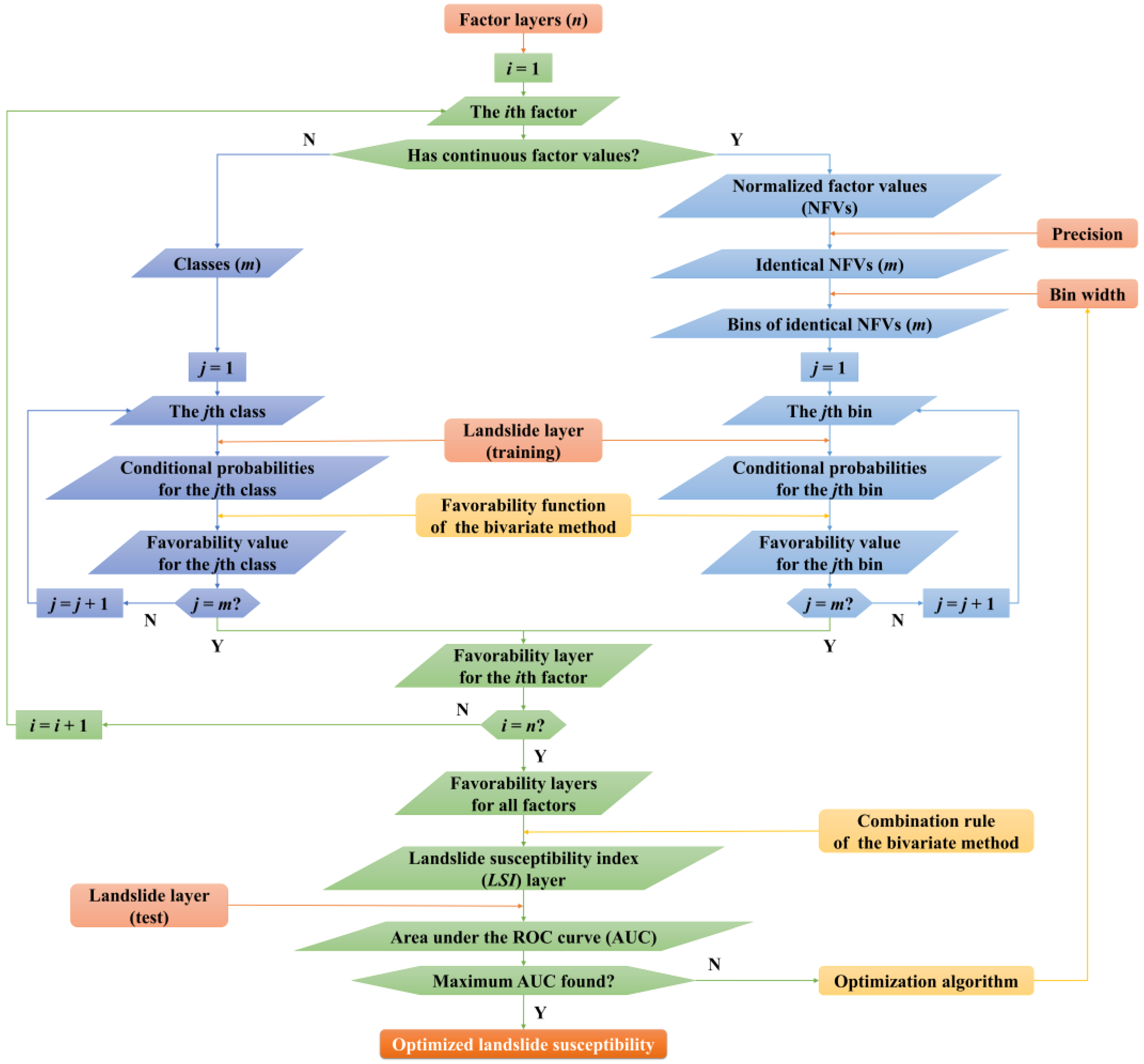
Differentiation of factor types. If the factor has classified values, go to step (2). If the factor has continuous factor values, go to step (3).

(2)

Generation of favorability layers for factors with classified values. First, empirical conditional probabilities for each class are derived based on the training landslide dataset. Then, favorability values for each class are calculated according to the favorability function of the bivariate method. Finally, a favorability layer for this factor with classified values can be produced based on favorability values for all classes.

(3)

Generation of favorability layers for factors with continuous factor values. This step is the core of classification-free modification.

First, continuous factor values are normalized to the 0–1 range. This normalization enables using the same parameters for different factors in the following procedures.

Second, a parameter, “precision”, which defines the number of digits after the decimal point, is applied to obtain identical normalized factor values. For example, if precision is 3, the normalized factor values 0.21237 and 0.21193 will both change to an identical normalized factor value of 0.212, and there will be, at most, 1001 identical normalized factor values. The application of precision can reduce the calculation loads by reducing the count of identical normalized factor values. It must be emphasized that precision setting is not obligatory, and a value of 0 means no precision will be applied, which further means that a favorability value will be calculated for each factor value within the study area.

Third, a bin is created for each identical normalized factor value, which centers at this value and has a width defined by the parameter “bin width”. This bin width ranges between 0 and 1 since factor values have been normalized. Bins of neighboring identical normalized factor values may have overlaps and can also have gaps if a low precision and a small bin width are adopted. The minimum effective bin width is determined by precision. For example, if precision is 3, the minimum difference between two neighboring identical normalized factor values will be 0.001. Then, a bin width smaller than 0.002 will not be effective because it means that there will be only one identical normalized factor value within any bin.

The principal idea of this procedure is to use continuous bins instead of discrete classes to analyze landslide sensibilities. Therefore, we use the phrase “classification-free” to name this modification. Because bin width is the only obligatory parameter that needs to be defined by users, the subjectivities associated with manual classifications of factors with continuous factor values can be reduced. Therefore, the discontinuity and subjectivity problems introduced by classifications of factors in conventional bivariate methods are moderated by this classification-free modification. In addition, this classification-free modification also significantly reduces manual choices and labor, and therefore favors an automatic analysis of landslide susceptibility.

Finally, similar to those done for classified factors, empirical conditional probabilities and favorability values for each bin are obtained, based on which a favorability layer for this factor with continuous factor values can be produced.

(4)

Generation of the landslide susceptibility index (LSI) layer. After favorability layers for all factors are obtained, an LSI layer can be produced according to the combination rule of the bivariate method, which will be a simple direct summation except for the certainty factor and weight of evidence methods (Table 1). In addition, in the LSI layer, zero slope grid cells will be set to null to satisfy the flat-area physical constraint, which can also be achieved by setting null grid cells with a null aspect.

(5)

Optimization of landslide susceptibility analysis. An LSI layer with a maximum prediction rate, i.e., a maximum AUC evaluated using the test landslide dataset, will provide an optimal assessment of landslide susceptibility. Given the landslide layer and the factor layers, favorability layers for factors with classified values are determined, while the generation of favorability layers for factors with continuous factor values is controlled by precision and bin width. Therefore, precision and bin width control the generation of the LSI layer. Here, optimization is implemented by searching an optimal bin width that yields a maximum prediction rate for predefined precisions (Figure 3). There are two reasons for only optimizing bin width [12]. First, precision is enumerable and finite in count. Second, precision has been shown to have a minor effect on the optimal result. The derived landslide susceptibility is dominated by bin width. A case study has shown that a precision of 2 can yield nearly the same optimal result as those yielded by precisions of 3, 4, 5, and 6. It is, therefore, not necessary to use large precision in optimization, which will significantly prolong the processing time.

For the eight conditional-probability-based bivariate methods, the exclusive use of empirical conditional probabilities to calculate favorability values and LSI values enables a general application of classification-free modification and further optimization. For those bivariate methods that do not exclusively depend on empirical conditional probabilities, favorability values and landslide susceptibility results are not exclusively dominated by bin width, and therefore an optimization based on the single parameter bin width is not applicable. It is worth mentioning that other existing or new conditional-probability-based bivariate methods not presented in this study can also be incorporated into this general optimization framework (Figure 3).

4. Open Software

This paper herein presents the updated version 3.0 of the open software Automatic Landslide Susceptibility Analysis (ALSA), which implements the general optimization framework for conditional-probability-based bivariate methods (Figure 3). ALSA 3.0 is coded with C# and has two versions: an ArcGIS extension version developed using ArcObjects, and a standalone version developed using MapWinGIS and GDAL. Both versions of ALSA 3.0 are freely available (Please contact the authors or visit https://github.com/lilangping/alsa/). The interface of ALSA 3.0 is shown in Figure 4. The inputs and settings of ALSA 3.0 are briefly introduced as follows.

(1)

Landslide data. Landslide data can be either points or polygons. Weight setting is an option for the point landslide layer so that sizes (areas) of landslides can be represented. Landslide grid cells can be split into training and test datasets according to the predefined ratio. Pseudo random is an option so that it is possible to use the identical division of training and test datasets in different runs.

(2)

Predisposing factor data. Predisposing factor data must be in a raster format. The checkbox in front of a classified factor layer should be checked. If all factors are classified, i.e., all checkboxes are checked, inputs for precision and bin width, as well as optimization settings, will become disabled, which further means that conventional bivariate methods will be used.

(3)

Processing extent. A rectangular processing extent will be automatically inherited from the extent of a selected data layer. If a polygon layer is selected, the geometry of polygon features can be used as the processing extent, which is not necessarily a rectangle. Coordinate systems of the landslide data, the predisposing factor data, and the data defining the processing extent must be the same.

(4)

Processing parameters. Processing parameters include the cell size of output raster layers and precision and bin width for the classification-free modification. Inputs for precision and bin width will be enabled if there is at least one factor with continuous factor values, while bin width input will be disabled if optimization is chosen because an optimal bin width will be generated.

(5)

Bivariate methods. Alternatives are the eight conditional-probability-based bivariate methods, i.e., frequency contrast, frequency ratio, information value, certainty factor, cosine amplitude, the weight of evidence, weight contrast, and sufficiency ratio methods.

(6)

Optimization settings. Optimization settings will be enabled if there is at least one factor with continuous factor values. If optimization is chosen, settings for optimization precision will be enabled, and bin width input will be disabled because an optimal bin width will be generated.

(7)

Output settings. Users should define the directory for output files, and file names of output files, including that of the output LSI raster layer, will be automatically generated so that the inputs and settings can be indicated.

ALSA 3.0 outputs several files, including an LSI layer, the favorability layers for all factors, the favorability values for all classes and bins of identical normalized factor values of all factors, a log file, and some other intermediate files. The varied sensibilities to slope failures of different values (either discrete classes or continuous values) of individual predisposing factors can be explored based on the output favorability values. In addition, if optimization is chosen, a file recording all inspected bin widths and their corresponding AUCs will also be output, based on which users can explore variations of success rate and prediction rate with bin width.

5. Preliminary Comparison

5.1. Study Area and Data

The Hengduan Mountain region (HDMR) is chosen as the case study area to make a preliminary comparison between different conditional-probability-based bivariate methods. The HDMR is located in the southeastern, marginal part of the Tibetan Plateau (Figure 5). With the constraint of major active faults, six big deeply cut rivers, i.e., the Min, Dadu, Yalong, Jinsha, Lancang, and Nu rivers, flow almost parallelly from north to south across the HDMR (Figure 5). Lying between those parallelly distributed big rivers are high mountain ranges with reliefs as high as more than 5000 m (statistics based on a circular neighborhood with a 10 km radius). Those alternatingly distributed, north–south featuring big rivers and high mountain ranges traverse the east–west extending “Sichuan–Tibet Corridor” (Figure 5), obtaining the name “Hengduan”, which literally means “traverse” in Chinese.

Owing to the active tectonic movement and high topographic relief, the HDMR suffered from severe mountain hazards [43,44,45,46,47,48,49,50,51]. Typical recent devastating landslide events include the Baige landslide that occurred on October 11 and November 3, 2018 [52,53,54], the Xinmo landslide that occurred on June 24, 2017 [55,56,57], as well as landslides triggered by the 2013 Lushan earthquake [58,59,60] and the 2008 Wenchuan earthquake [61,62,63]. In addition, active landslides have also been widely detected in the HDMR [64,65,66], threatening lives, properties, and engineering projects at risk. Therefore, landslide susceptibility analysis is very important for the HDMR [5,67,68,69,70,71].

A total of 2632 landslides in the HDMR (Figure 5a), recorded in a geological disaster dataset of China [72] and available in a point form, are adopted in this study. Eight predisposing factors with continuous factor values are adopted in landslide susceptibility analysis, namely, elevation, slope, aspect, curvature, distance to fault, distance to river, distance to road, and average annual precipitation (Figure 6). The elevation, slope, aspect, and curvature data are derived from the SRTM DEM with a 30 m × 30 m spatial resolution. The fault data are extracted from the 1:500,000 geological map of China. The river and road data are extracted from the 1:1,000,000 national basic geographic information dataset of China [73]. The 1 km × 1 km grid precipitation data record the average annual precipitation from 1980 to 2015 [74].

Some predisposing factors with classified values, such as geology, geomorphology, and vegetation, also have important constraints on the spatial distribution of landslides. Nevertheless, in this case study, only factors with continuous factor values are considered, so that no factors with classified values will be involved in the application of optimal bivariate methods. That is to say, in landslide susceptibility analysis with optimal bivariate methods, only factors with continuous factor values will be used, and for conventional bivariate methods, only factors with classified values will be used. Then, the comparison between optimal and conventional bivariate methods will not be complicated by the joint use of identical data.

5.2. Results and Comparisons

Landslide susceptibility in the HDMR is assessed using the eight conditional-probability-based bivariate methods in both optimal and conventional manners. The ratio of training to test landslide grid cells is 70:30. The cell size of output raster layers is set to 1 km. According to Figure 3, because the parameter bin width will be optimized, precision becomes the only constraining parameter needed for selection in the application of optimal bivariate methods. Without loss of generality, precision is set to 3, which should be a representative value because previous studies have suggested that precision has a minor effect on the optimal result [12]. In applying conventional bivariate methods, classifications of factors with continuous factor values are needed in the first place. In this study, three classification scenarios are adopted, in which factors with continuous factor values are manually categorized into 10, 5, and 3 classes, respectively. Therefore, a total of 32 landslide susceptibility maps are produced for the HDMR: 8 using optimal bivariate methods and 24 (8 × 3) using conventional bivariate methods.

The prediction rate, i.e., AUC calculated with the test landslide dataset, is used to evaluate the performance of the landslide susceptibility model. The prediction rates of the 32 landslide susceptibility maps are shown in

Table 4. Prediction rates of the 32 landslide susceptibility maps produced in the case study.

Method		Prediction Rate
		Optimal	Conventional			Average
			10 Classes	5 Classes	3 Classes	Value	Percent Difference
Frequency contrast		0.8662952	0.8584045	0.8493557	0.8291332	0.8507972	0.51
Frequency ratio		0.8662952	0.8584045	0.8493557	0.8291332	0.8507972	0.51
Information value		0.8672740	0.8622345	0.8545712	0.8360119	0.8550229	0.02
Certainty factor		0.8675016	0.8622918	0.8548182	0.8360542	0.8551665	N.A.
Cosine amplitude		0.8431700	0.8217469	0.8314922	0.8103809	0.8266975	3.44
Weight of evidence		0.8575339	0.8531959	0.8482106	0.8280323	0.8467432	0.99
Weight contrast		0.8660074	0.8559619	0.8502049	0.8303770	0.8506378	0.53
Sufficiency ratio		0.8662463	0.8583069	0.8492890	0.8291290	0.8507428	0.52
Average	Value	0.8625405	0.8538184	0.8484122	0.8285315	N.A.
	Percent difference	N.A.	1.02	1.67	4.10

Note: For all scenarios, the certainty factor method has the highest prediction rates (bold numerical values), while the cosine amplitude method has the lowest prediction rates (italic numerical values). In addition, for the cosine amplitude method, the prediction rate in the 10 classes scenario is lower than that in the 5 classes scenario, which differs from other bivariate methods. Percent difference quantifies the relative difference of a value compared with the maximum value. N.A. means not applicable.

. Two major findings can be obtained.

(1)

Different conditional-probability-based bivariate methods have a very close or even the same performance. This observation supports the theoretical interpretation of the close correlations between different conditional-probability-based bivariate methods. The certainty factor method has the highest prediction rates, and the information value method has almost the same prediction rates, with a percent difference close to zero (0.02) (Table 4). The cosine amplitude method has the lowest prediction rates, with a percent decrease of 3.44 compared to the certainty factor method (Table 4). The other five methods, i.e., the frequency contrast, frequency ratio, weight of evidence, weight contrast, and sufficiency ratio methods, have almost the same prediction rates, which are also very close to those of the certainty factor method (percent decreases less than 1.00) (Table 4). Particularly, for all scenarios, the frequency contrast and frequency ratio methods have the same prediction rates (Table 4).

The minor differences between conditional-probability-based bivariate methods are also reflected by the spatial distribution pattern of landslide susceptibility. The eight landslide susceptibility maps produced using optimal bivariate methods are used for illustration (Figure 7). We can see that high-susceptibility areas are distributed in the southern and eastern margins of the HDMR, as well as in river valleys, according to the spatial distribution pattern of landslides (Figure 7). The important result is that, when illustrated with histogram equalization stretching, the spatial patterns of landslide susceptibility maps produced by different bivariate methods show no macroscopic differences (Figure 7). This is because the order of grid cells in the sequence of LSI values does not differ too much between different bivariate methods.

The above observation suggests that the enhancement in performance introduced by selecting bivariate methods is negligible. Therefore, in practice, other manners should be considered to improve landslide susceptibility analysis, for example, optimizing the use of the mapping unit [2,75,76], landslide data [77,78,79], and predisposing factors [80,81,82,83], as well as introducing expert knowledge [84,85]. In addition, because different conditional-probability-based bivariate methods have strong intrinsic correlations, studies that make comparisons between their performances [86,87,88,89,90] are worth a revisit.

Because different conditional-probability-based bivariate methods have very close performances without loss of generality, we recommend using the certainty factor method as a prior choice. The certainty factor method will produce LSI values ranging within (−1, 1) and having a threshold value of 0 (see Section 2.2). This characteristic will stand in all scenarios of application, regardless of the type of landslide data or the number of considered predisposing factors, and thus is an advantage for interpreting landslide susceptibility results. In other bivariate methods, LSI values do not have a symmetrical range, and the threshold will change with the number of considered factors, restricting direct comparisons among different case studies.

(2)

Optimal bivariate methods perform better than conventional bivariate methods. For all eight conditional-probability-based bivariate methods, the optimal model has higher prediction rates than the conventional models (Table 4). In the applications of conventional bivariate methods, scenarios with more factor classes generally have higher prediction rates (Table 4). The percent increases in the prediction rate of the optimal model are 1.02, 1.67, and 4.10, respectively, when compared with conventional models with 10, 5, and 3 factor classes (Table 4). This is consistent with the intuition that the more factor classes, the closer the conventional model is to the optimal model in terms of classification-free modification.

Variations of success rate and prediction rate compared to bin width during the optimization of bivariate methods are shown in Figure 8. The maximum prediction rates are the final prediction rates of optimal bivariate methods, and the bin widths where we have the maximum prediction rates are the optimal bin widths (Figure 8). Accordingly, the percentage increases in maximum prediction rates compared with mean values are 4.70, 4.70, 4.74, 4.75, 4.72, 35.17, 11.17, and 4.70 for the frequency contrast, frequency ratio, information value, certainty factor, cosine amplitude, weight of evidence, weight contrast, and sufficiency ratio methods, respectively. This observation suggests that automatically obtained optimal bin widths perform better than arbitrary choices. It is worth mentioning that for the cosine amplitude, the weight of evidence, and weight contrast methods, because the order of favorability values is not only determined by p(L|F_i,j) (see Section 2.3), varying patterns of success rate and prediction rate are different from those of the other five bivariate methods (Figure 8).

Another important advantage of optimal bivariate methods is the exceptional ability to reveal the sensibilities of different factor values to slope failures for individual predisposing factors. Conventional bivariate methods calculate favorability values for only a few factor classes, while optimal bivariate methods calculate favorability values for quite a few identical normalized factor values so that the variation in the favorability value with the factor value is more differentiable. If no precision is applied, a favorability value will be calculated for each factor value within the study area. Variations in the favorability value with factor values in the case study are shown using the certainty factor method in Figure 9, and detailed, quasi-continuous varying characteristics of favorability value are revealed. For example, we can tell that the favorability for landslide occurrences generally decreases with elevation and distance to roads (Figure 9), and, specifically, elevations lower than ~3000 m favor landslide occurrences (Figure 9a), and distances to roads smaller than ~2500 m favor landslide occurrences (Figure 9g).

6. Conclusions

In this paper, the names, principles, and correlations of bivariate methods are first clarified based on a comprehensive and in-depth survey. A total of eleven prevalent bivariate methods are identified, nominated, and elaborated in a general framework, constituting a well-structured bivariate method family. It is shown that all prevalent bivariate methods depend on empirical conditional probabilities of landslide occurrence to calculate landslide susceptibilities, either exclusively or inclusively. It is clarified that those eight conditional-probability-based bivariate methods, which exclusively depend on empirical conditional probabilities, are particularly strongly correlated in principle and are therefore expected to have a very close or even the same performance.

It is also suggested that conditional-probability-based bivariate methods can apply a classification-free modification, in which factor classifications are avoided, and the result is dominated by a single parameter, bin width. Then, a general optimization framework, which is based on the classification-free modification, is proposed for conditional-probability-based bivariate methods. Optimal bivariate methods do not need factor classifications and obtain optimum results by optimizing the single dominant parameter bin width. The open software Automatic Landslide Susceptibility Analysis (ALSA) is updated to implement the eight conditional-probability-based bivariate methods and the general optimization framework.

Finally, a case study is presented, which confirms the theoretical expectation that different conditional-probability-based bivariate methods have a very close or even the same performance, and shows that optimal bivariate methods perform better than conventional bivariate methods regarding both the prediction rate and the ability to reveal the quasi-continuous varying pattern of sensibilities to landslides for individual predisposing factors. Specifically, in the certainty factor method, landslide susceptibility values will be within the same symmetrical range with a threshold value in the middle, regardless of application scenarios; therefore, it is recommended as a prior choice to facilitate direct comparisons among different case studies.

It should be emphasized that the case study presents a specific comparison between the eight conditional-probability-based bivariate methods. Although the Hengduan Mountain region (HDMR) is a representative landslide-prone area, we suggest that more investigations on performances of bivariate methods regarding different study areas, scales of analysis, settings of predisposing conditions, and availabilities of landslide and factor data are needed to obtain more inclusive and representative conclusions. The principles and open software presented in this study provide theoretical and practical foundations for extensive applications and comprehensive explorations of bivariate methods in landslide susceptibility analysis.

References

1. Fell, R.; Corominas, J.; Bonnard, C.; Cascini, L.; Leroi, E.; Savage, W.Z. Guidelines for Landslide Susceptibility, Hazard and Risk Zoning for Land Use Planning. Eng. Geol. 2008, 102, 85–98. [Google Scholar] [CrossRef] [Green Version]
2. Li, L.; Lan, H. Integration of Spatial Probability and Size in Slope-Unit-Based Landslide Susceptibility Assessment: A Case Study. Int. J. Environ. Res. Public Health 2020, 17, 8055. [Google Scholar] [CrossRef] [PubMed]
3. Reichenbach, P.; Rossi, M.; Malamud, B.D.; Mihir, M.; Guzzetti, F. A Review of Statistically-Based Landslide Susceptibility Models. Earth-Sci. Rev. 2018, 180, 60–91. [Google Scholar] [CrossRef]
4. Corominas, J.; van Westen, C.; Frattini, P.; Cascini, L.; Malet, J.P.; Fotopoulou, S.; Catani, F.; Van Den Eeckhaut, M.; Mavrouli, O.; Agliardi, F.; et al. Recommendations for the Quantitative Analysis of Landslide Risk. Bull. Eng. Geol. Environ. 2014, 73, 209–263. [Google Scholar] [CrossRef] [Green Version]
5. Li, L.; Lan, H.; Guo, C.; Zhang, Y.; Li, Q.; Wu, Y. A Modified Frequency Ratio Method for Landslide Susceptibility Assessment. Landslides 2017, 14, 727–741. [Google Scholar] [CrossRef]
6. Chung, C.-J.F.; Fabbri, A.G. The Representation of Geoscience Information for Data Integration. Nat. Resour. Res. 1993, 2, 122–139. [Google Scholar] [CrossRef]
7. Dou, J.; Yunus, A.P.; Bui, D.T.; Sahana, M.; Chen, C.W.; Zhu, Z.; Wang, W.; Pham, B.T. Evaluating Gis-Based Multiple Statistical Models and Data Mining for Earthquake and Rainfall-Induced Landslide Susceptibility Using the Lidar Dem. Remote Sens. 2019, 11, 638. [Google Scholar] [CrossRef] [Green Version]
8. Korup, O.; Stolle, A. Landslide Prediction from Machine Learning. Geol. Today 2014, 30, 26–33. [Google Scholar] [CrossRef]
9. Liu, L.L.; Zhang, J.; Li, J.Z.; Huang, F.; Wang, L.C. A bibliometric Analysis of the Landslide Susceptibility Research (1999–2021). Geocart. Int. 2022; in press. [Google Scholar] [CrossRef]
10. Yang, Z.; Liu, C.; Nie, R.; Zhang, W.; Zhang, L.; Zhang, Z.; Li, W.; Liu, G.; Dai, X.; Zhang, D.; et al. Research on Uncertainty of Landslide Susceptibility Prediction—Bibliometrics and Knowledge Graph Analysis. Remote Sens. 2022, 14, 3879. [Google Scholar] [CrossRef]
11. Süzen, M.L.; Doyuran, V. Data Driven Bivariate Landslide Susceptibility Assessment Using Geographical Information Systems: A Method and Application to Asarsuyu Catchment, Turkey. Eng. Geol. 2004, 71, 303–321. [Google Scholar] [CrossRef]
12. Zhang, Y.; Lan, H.; Li, L.; Wu, Y.; Chen, J.; Tian, N. Optimizing the Frequency Ratio Method for Landslide Susceptibility Assessment: A Case Study of the Caiyuan Basin in the Southeast Mountainous Area of China. J. Mt. Sci. 2020, 17, 340–357. [Google Scholar] [CrossRef]
13. Lee, S. Application of Likelihood Ratio and Logistic Regression Models to Landslide Susceptibility Mapping Using GIS. Environ. Manag. 2004, 34, 223–232. [Google Scholar] [CrossRef] [PubMed]
14. van Westen, C.J. Application of Geographic Information Systems to Landslide Hazard Zonation. Ph.D. Thesis, International Institute for Geo-Information Science and Earth Observation, Enschede, The Netherlands, 1993. Available online: http://www.itc.nl/library/Papers_1993/phd/vanwesten.pdf (accessed on 28 May 2022).
15. van Westen, C.J. Chapter 5: Statistical Landslide Hazard Analysis. In ILWIS Applications Guide; International Institute for Geo-Information Science and Earth Observation: Enschede, The Netherlands, 1997; pp. 73–84. Available online: https://www.itc.nl/ilwis/pdf/appch05.pdf (accessed on 4 August 2022).
16. Rautela, P.; Lakhera, R.C. Landslide Risk Analysis between Giri and Tons Rivers in Himachal Himalaya (India). Int. J. Appl. Earth Obs. Geoinf. 2000, 2, 153–160. [Google Scholar] [CrossRef]
17. Ghafoori, M.; Sadeghi, H.; Lashkaripour, G.R.; Alimohammadi, B. Landslide Hazard Zonation Using the Relative Effect Method. In The 10th IAEG International Congress (IAEG2006); Paper Number 474; The Geological Society of London: London, UK, 2006. [Google Scholar]
18. Lan, H.; Zhou, C.; Wang, L.; Zhang, H.; Li, R. Landslide Hazard Spatial Analysis and Prediction Using GIS in the Xiaojiang Watershed, Yunnan, China. Eng. Geol. 2004, 76, 109–128. [Google Scholar] [CrossRef]
19. Kanungo, D.P.; Arora, M.K.; Sarkar, S.; Gupta, R.P. A Comparative Study of Conventional, ANN Black Box, Fuzzy and Combined Neural and Fuzzy Weighting Procedures for Landslide Susceptibility Zonation in Darjeeling Himalayas. Eng. Geol. 2006, 85, 347–366. [Google Scholar] [CrossRef]
20. van Westen, C.J.; Rengers, N.; Soeters, R. Use of Geomorphological Information in Indirect Landslide Susceptibility Assessment. Nat. Hazards 2003, 30, 399–419. [Google Scholar] [CrossRef]
21. Constantin, M.; Bednarik, M.; Jurchescu, M.C.; Vlaicu, M. Landslide Susceptibility Assessment Using the Bivariate Statistical Analysis and the Index of Entropy in the Sibiciu Basin (Romania). Environ. Earth Sci. 2011, 63, 397–406. [Google Scholar] [CrossRef]
22. Bednarik, M.; Magulová, B.; Matys, M.; Marschalko, M. Landslide Susceptibility Assessment of the Kraľovany-Liptovský Mikuláš Railway Case Study. Phys. Chem. Earth 2010, 35, 162–171. [Google Scholar] [CrossRef]
23. Park, N.W. Application of Dempster-Shafer Theory of Evidence to GIS-Based Landslide Susceptibility Analysis. Environ. Earth Sci. 2011, 62, 367–376. [Google Scholar] [CrossRef]
24. An, P.; Moon, W.M.; Bonham-Carter, G.F. Uncertainty Management in Integration of Exploration Data Using the Belief Function. Nat. Resour. Res. 1994, 3, 60–71. [Google Scholar] [CrossRef]
25. Lee, S. Application and Verification of Fuzzy Algebraic Operators to Landslide Susceptibility Mapping. Environ. Geol. 2007, 52, 615–623. [Google Scholar] [CrossRef]
26. Peethambaran, B.; Anbalagan, R.; Shihabudheen, K.V. Landslide Susceptibility Mapping in and around Mussoorie Township Using Fuzzy Set Procedure, MamLand and Improved Fuzzy Expert System—A Comparative Study. Nat. Hazards 2019, 96, 121–147. [Google Scholar] [CrossRef]
27. Leonardi, G.; Palamara, R.; Cirianni, F. Landslide Susceptibility Mapping Using a Fuzzy Approach. Procedia Eng. 2016, 161, 380–387. [Google Scholar] [CrossRef]
28. Bonham-Carter, G.F.; Agterberg, F.P.; Wright, D.F. Weights of Evidence Modelling: A New Approach to Mapping Mineral Potential. In Statistical Applications in the Earth Sciences; Agterberg, G.F., Bonham-Carter, G.F., Eds.; Geological Survey of Canada: Ottawa, ON, Canada, 1989; pp. 171–183. [Google Scholar]
29. Regmi, N.R.; Giardino, J.R.; Vitek, J.D. Modeling Susceptibility to Landslides Using the Weight of Evidence Approach: Western Colorado, USA. Geomorphology 2010, 115, 172–187. [Google Scholar] [CrossRef]
30. Lee, S.; Min, K. Statistical Analysis of Landslide Susceptibility at Yongin, Korea. Environ. Geol. 2001, 40, 1095–1113. [Google Scholar] [CrossRef]
31. Denœux, T. 40 Years of Dempster–Shafer Theory. Int. J. Approx. Reason. 2016, 79, 1–6. [Google Scholar] [CrossRef]
32. Kanungo, D.P.; Sarkar, S.; Sharma, S. Combining Neural Network with Fuzzy, Certainty Factor and Likelihood Ratio Concepts for Spatial Prediction of Landslides. Nat. Hazards 2011, 59, 1491–1512. [Google Scholar] [CrossRef]
33. Akgun, A. A Comparison of Landslide Susceptibility Maps Produced by Logistic Regression, Multi-Criteria Decision, and Likelihood Ratio Methods: A Case Study at İzmir, Turkey. Landslides 2012, 9, 93–106. [Google Scholar] [CrossRef]
34. Bonham-Carter, G.F. Geographic Information Systems for Geoscientists: Modelling with GIS; Pergamon (Elsevier Science Ltd.): Kidlington, UK, 1994. [Google Scholar] [CrossRef]
35. Trigila, A.; Iadanza, C.; Spizzichino, D. Quality Assessment of the Italian Landslide Inventory Using GIS Processing. Landslides 2010, 7, 455–470. [Google Scholar] [CrossRef]
36. Shahabi, H.; Hashim, M. Landslide Susceptibility Mapping Using GIS-Based Statistical Models and Remote Sensing Data in Tropical Environment. Sci. Rep. 2015, 5, 9899. [Google Scholar] [CrossRef] [PubMed] [Green Version]
37. Shortliffe, E.H.; Buchanan, B.G. A Model of Inexact Reasoning in Medicine. Math. Biosci. 1975, 23, 351–379. [Google Scholar] [CrossRef]
38. Heckerman, D. Probabilistic Interpretations for Mycin’s Certainty Factors. Mach. Intell. Pattern Recogn. 1986, 4, 167–196. [Google Scholar] [CrossRef]
39. Ross, T.J. Fuzzy Logic with Engineering Applications, 4th ed.; Wiley: West Sussex, UK, 2017. [Google Scholar]
40. Neuhäuser, B.; Terhorst, B. Landslide Susceptibility Assessment Using “Weights-of-Evidence” Applied to a Study Area at the Jurassic Escarpment (SW-Germany). Geomorphology 2007, 86, 12–24. [Google Scholar] [CrossRef]
41. Carranza, E.J.M.; Hale, M. Evidential belief functions for data-driven geologically constrained mapping of gold potential, Baguio district, Philippines. Ore Geol. Rev. 2003, 22, 117–132. [Google Scholar] [CrossRef]
42. Zhu, A.X.; Wang, R.; Qiao, J.; Qin, C.Z.; Chen, Y.; Liu, J.; Du, F.; Lin, Y.; Zhu, T. An Expert Knowledge-Based Approach to Landslide Susceptibility Mapping Using GIS and Fuzzy Logic. Geomorphology 2014, 214, 128–138. [Google Scholar] [CrossRef]
43. Yang, Q.; Zheng, D.; Liu, Y. Physico-geographical feature and economic development of the dry valleys in the Hengduan Mountains, southwest China (in Chinese with English abstract). J. Arid Land Resour. Environ. 1988, 2, 17–24. [Google Scholar] [CrossRef]
44. Lan, H.; Wu, F.; Zhou, C.; Wang, L. Spatial hazard analysis and prediction on rainfall-induced landslide using GIS. Chin. Sci. Bull. 2003, 48, 703–708. [Google Scholar] [CrossRef]
45. Lan, H.; Zhang, N.; Li, L.; Tian, N.; Zhang, Y.; Liu, S.; Lin, G.; Tian, C.; Wu, Y.; Yao, J.; et al. Risk analysis of major engineering geological hazards for Sichuan-Tibet railway in the phase of feasibility study (in Chinese with English abstract). J. Eng. Geol. 2021, 29, 326–341. [Google Scholar] [CrossRef]
46. Lan, H.; Tian, N.; Li, L.; Liu, H.; Peng, J.; Cui, P.; Zhou, C.; Macciotta, R.; Clague, J.J. Poverty Control Policy May Affect the Transition of Geological Disaster Risk in China. Humanit. Soc. Sci. Commun. 2022, 9, 80. [Google Scholar] [CrossRef]
47. Meng, Y.; Lan, H.; Li, L.; Wu, Y.; Li, Q. Characteristics of Surface Deformation Detected by X-Band SAR Interferometry over Sichuan-Tibet Grid Connection Project Area, China. Remote Sens. 2015, 7, 12265–12281. [Google Scholar] [CrossRef] [Green Version]
48. Wei, L.; Hu, K.; Liu, S. Spatial Distribution of Debris Flow-Prone Catchments in Hengduan Mountainous Area in Southwestern China. Arab. J. Geosci. 2021, 14, 2650. [Google Scholar] [CrossRef]
49. Cui, P.; Ge, Y.; Li, S.; Li, Z.; Xu, X.; Zhou, G.G.D.; Chen, H.; Wang, H.; Lei, Y.; Zhou, L.; et al. Scientific Challenges in Disaster Risk Reduction for the Sichuan–Tibet Railway. Eng. Geol. 2022, 309, 106837. [Google Scholar] [CrossRef]
50. Li, J.; Liu, Z.; Wang, R.; Zhang, X.; Liu, X.; Yao, Z. Analysis of Debris Flow Triggering Conditions for Different Rainfall Patterns Based on Satellite Rainfall Products in Hengduan Mountain Region, China. Remote Sens. 2022, 14, 2731. [Google Scholar] [CrossRef]
51. Sun, X.; Zhang, G.; Wang, J.; Li, C.; Wu, S.; Li, Y. Spatiotemporal Variation of Flash Floods in the Hengduan Mountains Region Affected by Rainfall Properties and Land Use. Nat. Hazards 2022, 111, 465–488. [Google Scholar] [CrossRef]
52. Li, H.; Qi, S.; Chen, H.; Liao, H.; Cui, Y.; Zhou, J. Mass Movement and Formation Process Analysis of the Two Sequential Landslide Dam Events in Jinsha River, Southwest China. Landslides 2019, 16, 2247–2258. [Google Scholar] [CrossRef]
53. Yang, W.; Wang, Y.; Sun, S.; Wang, Y.; Ma, C. Using Sentinel-2 Time Series to Detect Slope Movement before the Jinsha River Landslide. Landslides 2019, 16, 1313–1324. [Google Scholar] [CrossRef]
54. Chen, Z.; Chen, S.; Wang, L.; Zhong, Q.; Zhang, Q.; Jin, S. Back Analysis of the Breach Flood of the “11.03” Baige Barrier Lake at the Upper Jinsha River (in Chinese with English abstract). Sci. Sin. Technol. 2020, 50, 763–774. [Google Scholar] [CrossRef]
55. Fan, X.; Xu, Q.; Scaringi, G.; Dai, L.; Li, W.; Dong, X.; Zhu, X.; Pei, X.; Dai, K.; Havenith, H.B. Failure Mechanism and Kinematics of the Deadly June 24th 2017 Xinmo Landslide, Maoxian, Sichuan, China. Landslides 2017, 14, 2129–2146. [Google Scholar] [CrossRef]
56. Ouyang, C.; Zhao, W.; He, S.; Wang, D.; Zhou, S.; An, H.; Wang, Z.; Cheng, D. Numerical Modeling and Dynamic Analysis of the 2017 Xinmo Landslide in Maoxian County, China. J. Mt. Sci. 2017, 14, 1701–1711. [Google Scholar] [CrossRef]
57. Shao, C.; Li, Y.; Lan, H.; Li, P.; Zhou, R.; Ding, H.; Yan, Z.; Dong, S.; Yan, L.; Deng, T. The Role of Active Faults and Sliding Mechanism Analysis of the 2017 Maoxian Postseismic Landslide in Sichuan, China. Bull. Eng. Geol. Environ. 2019, 78, 5635–5651. [Google Scholar] [CrossRef]
58. Tang, C.; Ma, G.; Chang, M.; Li, W.; Zhang, D.; Jia, T.; Zhou, Z. Landslides Triggered by the 20 April 2013 Lushan Earthquake, Sichuan Province, China. Eng. Geol. 2015, 187, 45–55. [Google Scholar] [CrossRef]
59. Xu, C.; Xu, X.; Shyu, J.B.H. Database and Spatial Distribution of Landslides Triggered by the Lushan, China Mw 6.6 Earthquake of 20 April 2013. Geomorphology 2015, 248, 77–92. [Google Scholar] [CrossRef] [Green Version]
60. Yang, Z.; Lan, H.; Gao, X.; Li, L.; Meng, Y.; Wu, Y. Urgent Landslide Susceptibility Assessment in the 2013 Lushan Earthquake-Impacted Area, Sichuan Province, China. Nat. Hazards 2015, 75, 2467–2487. [Google Scholar] [CrossRef]
61. Yin, Y.; Wang, F.; Sun, P. Landslide Hazards Triggered by the 2008 Wenchuan Earthquake, Sichuan, China. Landslides 2009, 6, 139–152. [Google Scholar] [CrossRef]
62. Qi, S.; Xu, Q.; Lan, H.; Zhang, B.; Liu, J. Spatial Distribution Analysis of Landslides Triggered by 2008.5.12 Wenchuan Earthquake, China. Eng. Geol. 2010, 116, 95–108. [Google Scholar] [CrossRef]
63. Zhang, Y.; Cheng, Y.; Yin, Y.; Lan, H.; Wang, J.; Fu, X. High-Position Debris Flow: A Long-Term Active Geohazard after the Wenchuan Earthquake. Eng. Geol. 2014, 180, 45–54. [Google Scholar] [CrossRef]
64. Liu, X.; Zhao, C.; Zhang, Q.; Lu, Z.; Li, Z.; Yang, C.; Zhu, W.; Jing, L.; Chen, L.; Liu, C. Integration of Sentinel-1 and ALOS/PALSAR-2 SAR Datasets for Mapping Active Landslides along the Jinsha River Corridor, China. Eng. Geol. 2021, 284, 106033. [Google Scholar] [CrossRef]
65. Zhang, J.; Zhu, W.; Cheng, Y.; Li, Z. Landslide Detection in the Linzhi–Ya’an Section along the Sichuan–Tibet Railway Based on InSAR and Hot Spot Analysis Methods. Remote Sens. 2021, 13, 3566. [Google Scholar] [CrossRef]
66. Yao, J.; Lan, H.; Li, L.; Cao, Y.; Wu, Y.; Zhang, Y.; Zhou, C. Characteristics of a Rapid Landsliding Area along Jinsha River Revealed by Multi-Temporal Remote Sensing and Its Risks to Sichuan-Tibet Railway. Landslides 2022, 19, 703–718. [Google Scholar] [CrossRef]
67. Sun, X.; Chen, J.; Li, Y.; Rene, N.N. Landslide Susceptibility Mapping along a Rapidly Uplifting River Valley of the Upper Jinsha River, Southeastern Tibetan Plateau, China. Remote Sens. 2022, 14, 1730. [Google Scholar] [CrossRef]
68. Wu, R.; Zhang, Y.; Guo, C.; Yang, Z.; Tang, J.; Su, F. Landslide Susceptibility Assessment in Mountainous Area: A Case Study of Sichuan–Tibet Railway, China. Environ. Earth Sci. 2020, 79, 157. [Google Scholar] [CrossRef]
69. Wang, S.; Zhuang, J.; Mu, J.; Zheng, J.; Zhan, J.; Wang, J.; Fu, Y. Evaluation of Landslide Susceptibility of the Ya’an–Linzhi Section of the Sichuan–Tibet Railway Based on Deep Learning. Environ. Earth Sci. 2022, 81, 250. [Google Scholar] [CrossRef]
70. Wu, W.; Zhang, Q.; Singh, V.P.; Wang, G.; Zhao, J.; Shen, Z.; Sun, S. A Data-Driven Model on Google Earth Engine for Landslide Susceptibility Assessment in the Hengduan Mountains, the Qinghai–Tibetan Plateau. Remote Sens. 2022, 14, 4662. [Google Scholar] [CrossRef]
71. Zhao, J.; Zhang, Q.; Wang, D.; Wu, W.; Yuan, R. Machine Learning-Based Evaluation of Susceptibility to Geological Hazards in the Hengduan Mountains Region, China. Int. J. Disaster Risk Sci. 2022, 13, 305–316. [Google Scholar] [CrossRef]
72. Geological Disaster Dataset of China; RESDC (Resource and Environment Science and Data Center). 2020. Available online: https://www.resdc.cn/data.aspx?DATAID=290 (accessed on 29 October 2020).
73. 1:1M National Basic Geographic Information Dataset of China; NCSFGI (National Catalogue Service for Geographic Information). 2018. Available online: https://www.webmap.cn/commres.do?method=result100W (accessed on 11 September 2018).
74. Spatial Interpolation Dataset of Annual Precipitation Since 1980 of China; RESDC (Resource and Environment Science and Data Center). 2019. Available online: https://www.resdc.cn/data.aspx?DATAID=229 (accessed on 15 August 2019).
75. Canavesi, V.; Segoni, S.; Rosi, A.; Ting, X.; Nery, T.; Catani, F.; Casagli, N. Different Approaches to Use Morphometric Attributes in Landslide Susceptibility Mapping Based on Meso-Scale Spatial Units: A Case Study in Rio de Janeiro (Brazil). Remote Sens. 2020, 12, 1826. [Google Scholar] [CrossRef]
76. Huang, F.; Tao, S.; Li, D.; Lian, Z.; Catani, F.; Huang, J.; Li, K.; Zhang, C. Landslide Susceptibility Prediction Considering Neighborhood Characteristics of Landslide Spatial Datasets and Hydrological Slope Units Using Remote Sensing and GIS Technologies. Remote Sens. 2022, 14, 4436. [Google Scholar] [CrossRef]
77. Hussin, H.Y.; Zumpano, V.; Reichenbach, P.; Sterlacchini, S.; Micu, M.; van Westen, C.; Bălteanu, D. Different Landslide Sampling Strategies in a Grid-Based Bi-Variate Statistical Susceptibility Model. Geomorphology 2016, 253, 508–523. [Google Scholar] [CrossRef]
78. Shu, H.; Guo, Z.; Qi, S.; Song, D.; Pourghasemi, H.R.; Ma, J. Integrating Landslide Typology with Weighted Frequency Ratio Model for Landslide Susceptibility Mapping: A Case Study from Lanzhou City of Northwestern China. Remote Sens. 2021, 13, 3623. [Google Scholar] [CrossRef]
79. Yang, X.; Liu, R.; Yang, M.; Chen, J.; Liu, T.; Yang, Y.; Chen, W.; Wang, Y. Incorporating Landslide Spatial Information and Correlated Features among Conditioning Factors for Landslide Susceptibility Mapping. Remote Sens. 2021, 13, 2166. [Google Scholar] [CrossRef]
80. Qin, C.Z.; Bao, L.L.; Zhu, A.X.; Wang, R.X.; Hu, X.M. Uncertainty Due to DEM Error in Landslide Susceptibility Mapping. Int. J. Geogr. Inf. Sci. 2013, 27, 1364–1380. [Google Scholar] [CrossRef]
81. Luti, T.; Segoni, S.; Catani, F.; Munaf, M.; Casagli, N. Integration of Remotely Sensed Soil Sealing Data in Landslide Susceptibility Mapping. Remote Sens. 2020, 12, 1486. [Google Scholar] [CrossRef]
82. Liu, Y.; Zhang, W.; Zhang, Z.; Xu, Q.; Li, W. Risk Factor Detection and Landslide Susceptibility Mapping Using Geo-Detector and Random Forest Models: The 2018 Hokkaido Eastern Iburi Earthquake. Remote Sens. 2021, 13, 1157. [Google Scholar] [CrossRef]
83. Barbosa, N.; Andreani, L.; Gloaguen, R.; Ratschbacher, L. Window-Based Morphometric Indices as Predictive Variables for Landslide Susceptibility Models. Remote Sens. 2021, 13, 451. [Google Scholar] [CrossRef]
84. Thiery, Y.; Maquaire, O.; Fressard, M. Application of Expert Rules in Indirect Approaches for Landslide Susceptibility Assessment. Landslides 2014, 11, 411–424. [Google Scholar] [CrossRef]
85. Yu, L.; Zhou, C.; Wang, Y.; Cao, Y.; Peres, D.J. Coupling Data- and Knowledge-Driven Methods for Landslide Susceptibility Mapping in Human-Modified Environments: A Case Study from Wanzhou County, Three Gorges Reservoir Area, China. Remote Sens. 2022, 14, 774. [Google Scholar] [CrossRef]
86. Mohammady, M.; Pourghasemi, H.R.; Pradhan, B. Landslide Susceptibility Mapping at Golestan Province, Iran: A Comparison between Frequency Ratio, Dempster-Shafer, and Weights-of-Evidence Models. J. Asian Earth Sci. 2012, 61, 221–236. [Google Scholar] [CrossRef]
87. Guo, C.; Montgomery, D.R.; Zhang, Y.; Wang, K.; Yang, Z. Quantitative Assessment of Landslide Susceptibility along the Xianshuihe Fault Zone, Tibetan Plateau, China. Geomorphology 2015, 248, 93–110. [Google Scholar] [CrossRef]
88. Hong, H.; Chen, W.; Xu, C.; Youssef, A.M.; Pradhan, B.; Tien Bui, D. Rainfall-Induced Landslide Susceptibility Assessment at the Chongren Area (China) Using Frequency Ratio, Certainty Factor, and Index of Entropy. Geocart. Int. 2017, 32, 139–154. [Google Scholar] [CrossRef]
89. Wang, Q.; Guo, Y.; Li, W.; He, J.; Wu, Z. Predictive Modeling of Landslide Hazards in Wen County, Northwestern China Based on Information Value, Weights-of-Evidence, and Certainty Factor. Geomat. Nat. Hazards Risk 2019, 10, 820–835. [Google Scholar] [CrossRef] [Green Version]
90. Kavoura, K.; Sabatakakis, N. Investigating Landslide Susceptibility Procedures in Greece. Landslides 2020, 17, 127–145. [Google Scholar] [CrossRef]
Figure 1. Clarification of bivariate methods of landslide susceptibility analysis. (a) Unstructured bivariate method family (before clarification) is illustrated with a relationship network. Larger dots indicate methods with higher frequencies of occurrence in titles and abstracts of publications with a topic of landslide susceptibility, and thicker lines indicate higher frequencies of co-occurrence. Data of publications were accessed from the Web of Science Core Collection on 19 July 2022. (b) The well-structured bivariate method family (after clarification) is illustrated with a table. The eight conditional-probability-based methods exclusively, and other methods inclusively, depend on empirical conditional probabilities of landslide occurrence. Details of conditional probabilities are referred to in the main text (Section 2.2). The 8 conditional-probability-based methods, which are the main focus of this contribution, are summarized in Table 1 and detailed in Section 2.2.3. The 3 other bivariate methods are briefly introduced in Section 2.2.4.
Remotesensing 15 01418 g001
Figure 2. General steps of conditional-probability-based bivariate methods.
Remotesensing 15 01418 g002
Figure 3. General optimization framework for conditional-probability-based bivariate methods of landslide susceptibility analysis.
Remotesensing 15 01418 g003
Figure 4. Interface of ALSA (Automatic Landslide Susceptibility Analysis) 3.0.
Remotesensing 15 01418 g004
Figure 5. Hengduan Mountain region (HDMR). Landslides used in susceptibility analysis are shown in (a). Location of the HDMR relative to the Tibetan Plateau is shown in (b).
Remotesensing 15 01418 g005
Figure 6. Predisposing factors with continuous factor values adopted in the case study. (a) Elevation. (b) Slope. (c) Aspect. (d) Curvature. (e) Distance to fault. (f) Distance to river. (g) Distance to road. (h) Average annual precipitation. Histogram equalization stretching is used in illustrations of factor values.
Remotesensing 15 01418 g006
Figure 7. Landslide susceptibility maps produced using optimal bivariate methods in the case study. (a) The frequency contrast method. (b) The frequency ratio method. (c) The information value method. (d) The certainty factor method. (e) The cosine amplitude method. (f) The weight of evidence method. (g) The weight contrast method. (h) The sufficiency ratio method. Histogram equalization stretching is used in illustrations of landslide susceptibility index (LSI) values.
Remotesensing 15 01418 g007
Figure 8. Variations in success rate and prediction rate with bin width during the optimization of bivariate methods in the case study. (a) The frequency contrast method. (b) The frequency ratio method. (c) The information value method. (d) The certainty factor method. (e) The cosine amplitude method. (f) The weight of evidence method. (g) The weight contrast method. (h) The sufficiency ratio method.
Remotesensing 15 01418 g008
Figure 9. Variations in favorability value with factor values in the case study are shown using the certainty factor method. (a) Elevation. (b) Slope. (c) Aspect. (d) Curvature. (e) Distance to fault. (f) Distance to river. (g) Distance to road. (h) Average annual precipitation.
Remotesensing 15 01418 g009