Abstract
The diffuse attenuation coefficient for the downwelling irradiance is a critical parameter in terms of the optical properties of the ocean. In the northwestern South China Sea, there are complex physical processes, and the accurate estimation of in the northwestern South China Sea is critical for the study and application of the underwater light field and water constituents. In this study, using Hydrolight 6.0 (HL60) software, was simulated based on the inherent optical properties (IOPs) and chlorophyll a concentration dataset in the northwestern South China Sea. The simulations were in good agreement with the results calculated by the model of Lee (2005), and the spectral characteristics of were consistent with several oceanic types according to Jerlov’s classification. The horizontal and vertical distribution characteristics of were studied in the two typical upwelling areas of eastern Hainan Island and eastern Vietnam. in eastern Hainan Island exhibited an overall decreasing trend from west to east at the same depth, while the vertical depth of the maximum value of in eastern Hainan Island was found to increase from west to east, which was significantly associated with the distribution trend of the temperature and salinity. in eastern Vietnam exhibited unique horizontal and vertical distribution characteristics due to upwelling, with a low temperature and high salinity. A satisfactory linear relationship between and was found from with > 0.76, root mean square (RMSE) 0.010 , and mean absolute percentage error (MAPE) < 9%, and this result indicated that from could be estimated with . The regression accuracy sharply decreased after 580 nm, indicating that estimation based on can be more suitably achieved from 420~580 nm and becomes inaccurate after 580 nm. Based on the simulations, an empirical relationship for estimation involving was developed, and in the northwestern South China Sea was calculated, with a range of 5–23 m and a suitable agreement with obtained via the method of Lee (2018).
1. Introduction
The diffuse attenuation coefficient for the downwelling irradiance, as a function of the depth, , and wavelength, can be used to characterize the decrease in the ambient downwelling irradiance, [1]. This parameter can be defined as [2]:
where and denote two profile depths that are very near to each other.
For , cannot be calculated with Equation (1) [3]. denotes the downwelling irradiance just above the surface.
This quantity has been considered one of the key indicators to describe the attenuation of the downwelling solar radiation within the water column, as well as a critical factor for the Secchi disk depth (SDD) and euphotic zone depth [4]. All these parameters are important in studying the underwater photovoltaic (PV) power generation [5], heat budget of the oceanic mixed layer [6], photosynthesis of phytoplankton, and warning of harmful algal blooms [7,8].
The South China Sea (SCS) is the largest trophic marginal sea in the western Pacific Ocean, and it plays an important role in regulating the regional climate and carbon cycle with its extensive area and volume [9,10]. In the northwestern South China Sea, there are physical processes such as Qiongdong upwelling, eastern Vietnam upwelling, western Guangdong coastal currents, freshwater from the Pearl River estuary, and some subtropical bay influenced by human activity [11]. These processes lead to complex physical and biochemical changes in the northwestern South China Sea. The accurate estimation of and its distribution in the northwestern South China Sea is critical for the study and application of the underwater light field and water constituents [7].
At present, can be obtained via in situ measurements, empirical algorithms, semi-analytical algorithms, and analytical algorithms [3,12,13].
Regarding in situ measurements, a profile of the downwelling irradiance, , is first obtained from instrumentation, and can then be calculated via Equation (1). In situ measurements are generally classified into two types: (1) surface radiation measurements based on optical buoy platforms and (2) profile radiation measurements involving radiometer profilers. Because irradiance measurement is very sensitive to radiometer self-shading, platform stability, and environmental factors such as clouds, aerosols, and solar radiation, it is difficult to control the data quality of in situ measurements [14,15,16].
In empirical algorithms, the diffuse attenuation coefficient is directly described as a function of the ratio of the water-leaving radiance or remote-sensing reflectance between several different wavelengths. In 1981, based on the water-leaving radiance retrieved from Coastal Zone Color Scanner (CZCS) data, Austin et al. [17] built an empirical relationship between and the ratio between the blue and green water-leaving radiances. Subsequently, to provide a high accuracy and regional adaptability, the empirical relationship determined by Austin et al. was improved and optimized [18,19,20]. In 2020, based on time series optical buoy data, according to the favorable correlation of the and band ratios with / and /, a dual-band ratio empirical algorithm for was established by Zhang et al. [21], and this algorithm is superior to other empirical algorithms because the selected by this algorithm can fully reflect water body information and can be adapted to changes in the water composition in the study sea area. All these empirical algorithms are easy in operation and beneficial to calculate the at a large spatial scale in the surface, but they are limited in accuracy and generalization and cannot explain the variation of and the underwater light field.
To overcome the disadvantages of empirical algorithms, based on the radiative transfer equation (RTE), several analytical and semi-analytical algorithms for estimation have been proposed. In 1976, Preisendorfer [22] established a comprehensive theoretical framework for ocean color and radiative transfer. Analytical algorithms were built based on the RTE, while the developed semi-analytical algorithms were based on the simplified RTE [23,24,25]. Based on the RTE and the increasing computing ability, a numerical simulation model, namely Hydrolight, was established by Mobley [26] in 1994. Hydrolight provides exact solutions to estimate the apparent optical properties (AOPs: diffuse attenuation coefficient , remote sensing reflectance , etc.) from the inherent optical properties (IOPs: absorption coefficient , attenuation coefficient , volume scattering function , etc.) [8], and this model is a powerful tool to study underwater light fields, facilitating progress in the study of the ocean primary productivity, ocean color remote sensing, environmental and ecological changes, and global energy cycles [2,27,28]. With the use of Hydrolight numerical simulations, Huang et al. [29] constructed a remote sensing reflectance dataset for Taihu Lake and compared it to measured remote sensing reflectance spectra, and based on the RTE and Hydrolight numerical simulations, a semi-analytical model for was developed by Lee et al. [2], which is called the model of Lee (2005) in this study, and this model can estimate based on the absorption and backscattering coefficients, which could be adapted well to both oceanic and coastal waters. Based on the simulations, Lee et al. [2] constructed a look-up table (LUT) for the values of the model parameters at specific solar altitude and profile depth ranges.
Previous studies of the diffuse attenuation coefficient, especially , have been conducted in the South China Sea more notably involving empirical algorithms and in situ downward irradiance data than involving analytical algorithms, and the original input parameters include the remote sensing reflectance, Chla, and in situ radiometric measurement data [30,31,32]. Uncertainties exist in both in situ and satellite-derived measurements of . To address these issues, based on in situ measurements of the IOPs and boundary conditions such as the light field and meteorological parameters, the spectral and vertical distributions of in the northwestern South China Sea, especially the profile distribution characteristics in two typical upwelling regions, were studied via Hydrolight 6.0 (HL60) numerical simulations. Then, linear relationships between and were derived by regressing the simulation data, and the Secchi disk depth in the northwestern South China Sea was estimated via and . This study provides strong support for the evaluation of the underwater light field from IOPs.
2. Methods and Data
2.1. Hydrolight
Hydrolight solves the RTE using a numerical technique to compute the radiance distribution in a natural hydrosol based on the IOPs of the hydrosol itself and appropriate boundary conditions at the surface and bottom of the water body, along with the radiance incident on the water surface [33].
In this study, Hydrolight version 6.0 (HL60) was used to simulate diffuse attenuation coefficients such as and , based on the water IOPs and surface and bottom boundary conditions. In HL60, seven options are available for IOP input: Constant IOPs, Classic Case 1 IOPs, New Case 1 IOPs, Measured IOPs, Case 2 IOPs, New Case 2 IOPs, and A user-defined IOP Model. The option of Measured IOPs, in which it is assumed that IOPs comprise pure water values plus “everything else” (particles and dissolved substances) measured by ac-s (the Wetlabs (now Seabird, in Bellevue, WA, USA) underwater hyperspectral absorption and attenuation meter) [34], HS6 (the HOBI Laboratories (in Bellevue, WA, USA) HydroScat-6 spectral backscattering sensor and fluorometer) [35], or similar instruments, was selected in this study, and Pope and Fry’s pure water absorption and seawater scattering coefficients were used [36] for the pure water component. The absorption and attenuation coefficients for “everything else” were measured via ac-s, and the backscattering coefficients for “everything else” were obtained in situ via HS6. Regarding the Measured IOPs model, the total minus water absorption coefficient (), total minus water attenuation coefficient (), particulate backscattering coefficient (), and chlorophyll a concentration (Chla) are needed as inputs, a Fournier–Forand phase function with the given ratio is used to estimate the scattering phase function of particulate matter in HL60, and the particulate scattering coefficient () can be obtained by subtracting from . Vertical profiles of Chla() are needed to compute chlorophyll fluorescence effects. In addition, the effects of inelastic scatter by colored dissolved organic matter (CDOM) fluorescence and Raman scattering are needed and could be calculated via the default function in HL60. The sky radiance distribution could be obtained from a semiempirical model, which was built in HL60. Moreover, we used the Harrison and Coombes normalized sky radiance model and RADTRANX sky irradiance model to specify the distribution of the sky radiance and partition the total irradiance into diffuse and direct irradiance components, respectively. The bottom boundary was set to an infinite depth. Then, with these settings, within 26 wavebands between 420 and 670 nm, separated by 10 nm, and could be obtained in HL60. A simulation flowchart for HL60 is shown in Figure 1.
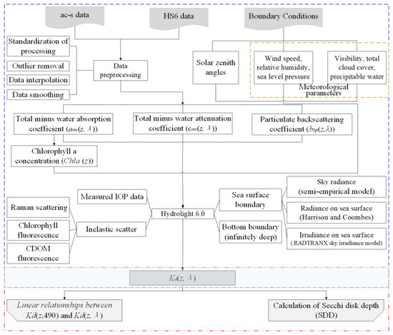
Figure 1.
Flowchart of this study.
2.2. Cruise and Sampling
Two cruises were carried out in the northwestern South China Sea to collect IOPs: 9 August to 2 September 2013 (cruise 2013) and 30 June to 17 July 2015 (cruise 2015). Figure 2 shows the locations of the sampling stations. These cruise datasets contain match-ups of vertical profiles of , , , and Chla() for 55 stations, along with the solar zenith angle, computed based on the time, latitude, and longitude of each station. These in situ measurements include a maximum depth in 99 m (offshore) and a minimum depth in 22 m (nearshore). Additionally, various meteorological parameters (e.g., wind speed and relative humidity) were collected simultaneously during sampling. The sampling area mainly involves two typical upwelling areas of eastern Hainan Island and eastern Vietnam with significant bio-optical variability and strong hydrodynamic processes.
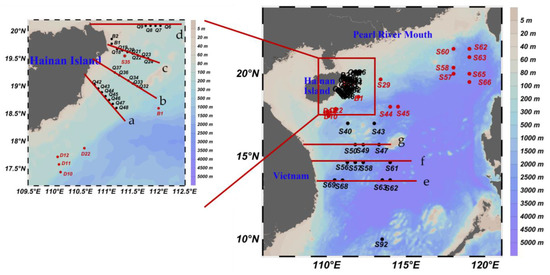
Figure 2.
Locations of the stations in the northwestern South China Sea. The black circles denote the stations during the 2013 cruise. The red circles denote the stations during the 2015 cruise. The red lines indicate the seven sections.
2.2.1. Absorption and Attenuation Measurements
Vertical profiles of the total minus water absorption coefficient () and total minus water attenuation coefficient () were measured via ac-s with 82 wavebands between 401.6 and 744.1 nm and a path length of 25 cm. Milli-Q ultrapure water was used to calibrate the drift of the ac-s instrument and as a reference blank before the cruises. To mitigate any temperature and salinity effects on the ac-s measurements, a simultaneous seabird conductivity–temperature–depth (CTD) sensor (SBE 911plus CTD) was used to obtain temperature and salinity profiles [37]. In addition, all measurements were corrected for scattering by setting the absorption values as zero near the infrared wavelengths (716 nm was used in this study) [38]. As such, first, outlier data, including data less than or equal to zero, data deviating from the normal range, and same data values at the same depth, were excluded. Then, using the piecewise cubic interpolation (pchip) method, the data were interpolated to a profile resolution of 1 m, and finally, the interpolation data were smoothed via the Savitzky–Golay filtering method [39].
2.2.2. Backscattering Measurements
Vertical profiles of the particulate backscattering coefficient () were obtained from the HS6 instrument. The HS6 instrument could be used to measure vertical profiles of the volume scattering function () at a single angle along the backward direction () at six wavelengths (420, 442, 488, 532, 590, and 676 nm). The measurement data were processed based on the standard processing procedure provided by HOBI Laboratories, and the following sequential steps were employed: correction for the dark current, conversion of the raw signal into values of the volume scattering function , improvement in the accuracy of via sigma correction based on the attenuation coefficient c, calculation of the particulate volume scattering function from under subtraction of the volume scattering function of seawater [40], and estimation of the particulate backscattering coefficient, , from multiplied by the relevant factor, [35]. Similarly, the same outlier removal, data interpolation, and smoothing processes were applied to the corrected data, similarly to the ac-s measurement data.
2.2.3. Chla Data
To correct for the effect of inelastic scatter of chlorophyll fluorescence, Chla() can be adopted as an input parameter. In this study, Chla() was calculated from using the absorption line height method (denoted as the aLH method) and a profile resolution of 1 m in accordance with the ac-s and HS-6 data.
Scholars have shown that there is a power function-based correlation between the absorption line height at and Chla() [41,42], and an absorption line height method (i.e., the aLH method) was developed for Chla() estimation from the absorption line height, , at [42]. The calculation process of the aLH method can be described as follows:
First, the absorption of the baseline at a reference wavelength, , of and can be calculated as:
Second, the absorption line height at 676 nm, , can be calculated from the difference between and as:
Finally, Chla() can be estimated from as follows:
where A and B are 108.07 and 1.084, respectively, in the South China Sea [43], and is the chlorophyll a concentration derived via the aLH method.
2.2.4. Surface Boundary Conditions
The solar zenith angle was computed based on the time, latitude, and longitude of each station. Wind speed, relative humidity, sea level pressure, etc., were collected at the same time as the IOP dataset. Visibility data were collected from a Global Atmospheric Reanalysis (CRA-40) dataset released by the China Meteorological Administration (CMA) (https://data.cma.cn/, accessed on 20 January 2023). The total cloud cover and precipitable water were obtained from the National Centers for Environmental Prediction (NCEP)/National Center for Atmospheric Research (NCAR) Reanalysis I dataset (https://psl.noaa.gov/data/gridded/data.ncep.reanalysis.html, accessed on 20 January 2023), and these reanalysis datasets were obtained by using a climate model to initialize a wide variety of weather observations (ship data, plane measurements, station data, satellite observations, etc.).
2.3. Accuracy Evaluation Indicators
To assess the performance of the results, the following statistical indicators were used: the coefficient of determination (), root mean square error (RMSE), and mean absolute percentage error (MAPE), which can be defined as follows:
where denotes the true value, denotes the estimated value, is the average true value, and is the number of data pairs.
3. Results and Applications
3.1. Spectral Characteristics of
Figure 3 shows the spectral distribution of simulated by HL60 in all 55 station profiles. As shown in Figure 3, the simulation results exhibited significant spectral and spatial distribution characteristics. The minimum value of generally appeared at approximately 490 nm, while the maximum value occurred at approximately 670 nm. According to Jerlov’s classification of water types (as shown in Figure 3b), the spectra of at these stations did not significantly differ from several oceanic types, especially type ΙB, type II, and type III [44]. There seem to be two different trends from 420–470 nm, one with an obvious downward trend and the other with a stabilized trend. The spectral characteristic with the obvious downward trend from 420–470 nm seems to occur in the nearshore stations. At all stations, tended to increase with the wavelength from 550 to 670 nm, with a sharp upward trend from 570 to 600 nm, while the upward trend started to decline from 600 to 670 nm.
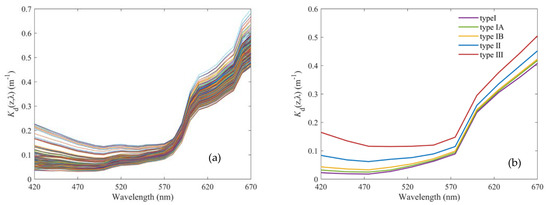
Figure 3.
Spectral characteristics of : (a) all stations of this study; (b) Jerlov’s oceanic water type.
3.2. Spatial and Vertical Distribution Characteristics of
Figure 4a–c show the depth–wavelength distribution of on stations B2 in 2013, Q45 in 2013, and S63 in 2015, which can represent three water types: turbid water, relatively clear water, and clear water. Among all these water types, there were very obvious wavelength distribution characteristics of in the vertical profile. Among all of the profiles shown, the magnitude of uniformly increased with increasing depth. The profile at approximately 590 nm was an exception to this trend, as the magnitude decreased with increasing depth, and this feature could be observed in all of the wavelength bands > 590 nm. As shown in Figure 4a, the spectral variation in of the vertical profile was obvious from 420~670 nm; at approximately 490 nm was the minimum at the surface, the minimum value then moved toward higher wavelengths with increasing vertical depth, the minimum of moved to 560 nm, and the water window did not involve 490 nm but 560 nm. As shown in Figure 4b,c, there occurred relatively little change in the minimum of from 420~670 nm in the vertical profile, and at approximately 490 nm indicated the greatest ability for penetration in seawater, which makes particularly unique in ocean color remote sensing, seawater transparency, and euphotic zone depth applications [33].
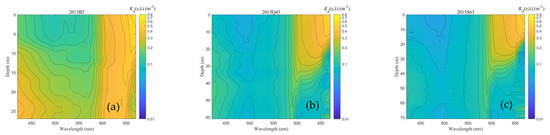
Figure 4.
Depth-wavelength distribution characteristics of : (a) station B2 in 2013 (water column depth: 35 m); (b) station Q45 in 2013 (water column depth: 107 m); (c) station S63 in 2015 (water column depth: 2716 m).
The spatial distribution of at the different water depths, including 0, 5, 10, 15, and 20 m, at all stations (all stations were surveyed to depths of more than 20 m but less than 25 m) is shown in Figure 5. Figure 5, Figure 6 and Figure 7 were generated by Ocean Data View (ODV), and the Weighted-average gridding method was used to interpolate the station values. The contours of in the five water layers revealed consistent spatial distribution characteristics. At all stations in the same vertical layer, exhibited a decreasing trend from nearshore to offshore. In the five water layers at the same station, indicated an increasing trend with increasing vertical depth, and the increase rate decreased with increasing offshore distance, i.e., the farther offshore, the gentler the change was. As shown in Figure 5, the contour lines significantly indicated that exhibited a decreasing trend with increasing offshore distance. The smaller the offshore distance to the same water layer, the denser the contour lines were and the more significant the spatial variation rate of was.
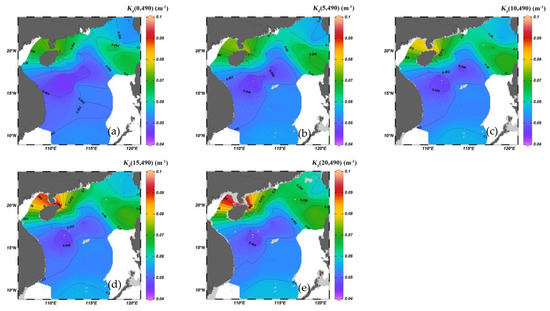
Figure 5.
Spatial distribution of at (a) 0 m, (b) 5 m, (c) 10 m, (d) 15 m, and (e) 20 m underwater.
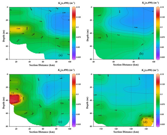
Figure 6.
Vertical and horizontal distributions of in eastern Hainan Island: (a) Section a, (b) section b, (c) section c, and (d) section d.
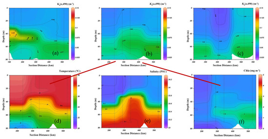
Figure 7.
Vertical and horizontal distributions of in the upwelling area of eastern Vietnam: (a) Section e, (b) section f, (c) section g, (d) temperature in section f, (e) salinity in section f, and (f) Chla in section f.
Four longitudinal sections (sections a, b, c, and d, as shown in Figure 2) in eastern Hainan Island were chosen to analyze the vertical and horizontal distribution characteristics of , as shown in Figure 6a–d. The spatial distribution characteristic of exhibited an overall decreasing trend from west to east at the same depth in longitudinal sections a, b, c, and d. There was a vertical profile maximum of in all sections. Moreover, the vertical depth of the maximum value of in sections a and c (as shown in Figure 6a,c, respectively) was found to increase from west to east, and the difference in the vertical depth of the maximum value of within the same section could exceed 20 m. Compared to that in sections a and c, there was a slight difference in the vertical maximum depth between the different stations in sections b and d, respectively, and the maximum depth reached approximately 50 m.
The vertical and horizontal distribution characteristics of in the upwelling area of eastern Vietnam (e, f, and g sections in Figure 2) are shown in Figure 7a–c. In these sections, revealed unique profile distribution characteristics in sections e, f, and g. The value of in section e followed the same trend as that in sections a–d, with larger values in the west and smaller values in the east, and the maximum vertical depths of were located at shallower depths in the west than in the east, with a depth difference of 20 m. The vertical depth of the maximum value of in section f showed a convex structure from west to east. In contrast to section f, the vertical depth of the maximum value of in section g showed a concave structure from west to east.
Overall, the vertical profile changes in were more significant in the nearshore area. In all of the above sections from a to g, the maximum value of reached approximately 0.14 at the Q18 station in section c, and the minimum value was 0.035 at the S49 station in section f.
3.3. Spectral Model of the Diffuse Attenuation Coefficient
Jerlov [44] proposed that could be expressed as a satisfactory linear function of , where is the reference wavelength (e.g., 475 or 490 nm), which helped researchers derive at one or more wavelengths from . Subsequently, based on in situ measurements, with the use of 490 nm as , researchers have constructed several models similar to the relationship proposed by Jerlov for different sea areas [31,45]. In our study, based on the function established by Austin et al. (Equation (8)) [45], relationships between and at were established via HL60 simulations.
As shown in Figure 8 and Figure 9, these relationships performed better between 420 and 580 nm, with , RMSE, and MAPE . of these linear relationships, centered at 490 nm, tended to first increase and then decrease with increasing wavelength, while RMSE and MAPE tended to first decrease and then increase with increasing wavelength. The closer was to 490 nm, the higher and the smaller RMSE and MAPE. The relationships performed the best at approximately 490 nm, with , RMSE , and MAPE at 450540 nm. However, the linear regression accuracy decreased obviously from 590 nm to higher wavelengths, with the value decreasing from 0.578 at 590 nm to 0.128 at 670 nm, which indicated that the estimation of based on is subject to a certain wavelength applicability range (420~580 nm). A poor quality of linear regression at higher wavelengths was previously reported by Austin et al. [45]. This result showed that to ensure the accuracy of estimation based on in the northwestern South China Sea, the wavelength should be chosen from 420~580 nm.
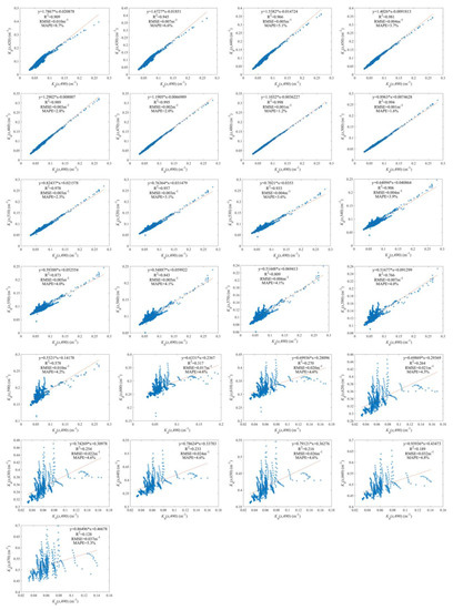
Figure 8.
Linear relationships between () and .
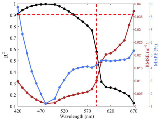
Figure 9.
Accuracy evaluation of the linear regression results.
We also found that coefficients and in Equation (8) from 420~580 nm could be described as quadratic functions of the wavelength via regression analysis. As shown in Figure 10, the quadratic regression accuracy of versus the wavelength indicated = 0.9995, RMSE = 0.009, and MAPE = 0.9%, and the regression of versus the wavelength achieved a higher accuracy with = 0.991, RMSE = 0.003, and MAPE = 18.9%.
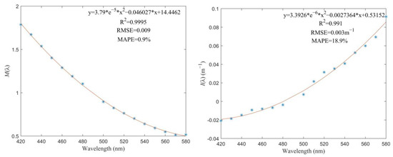
Figure 10.
Quadratic regression results between the various wavelengths and the linear regression results of (a) the slope coefficient and (b) intercept coefficient .
3.4. Algorithm for Estimation Based on the Diffuse Attenuation Coefficient
The Secchi disk depth (SDD) is an important parameter to describe the submarine optical field distribution and a key indicator in military–civilian integration fields, such as underwater target detection, communication, fishery production, and marine ecological environment monitoring [46,47,48]. Traditionally, SDD was measured by a white or black-and-white disk with a diameter generally about 30 cm [49]. A depth at which the Secchi disk is no longer visualized by an observer represents a quantitative measure of the transparency of ocean and lake waters. The traditional instrument is low cost and easy to operate [50], but it is limited in accuracy. Therefore, a series of regional algorithms or semi-analytical algorithms have been constructed in terms of the relationship between and [4,49]. In contrast, the euphotic zone depth () is the depth where 1% of the photosynthetically available radiation (PAR()) just beneath the water surface remains and is often quantified by the diffuse attenuation coefficient of the PAR() () [51].
where is the at the euphotic zone depth.
In the ocean color community, can be converted to via Equation (10).
where denotes the proportionality factor.
As reported by Austin et al. [52], attained a notable linear correlation with , and .
where is the slope of the linear regression equation.
In this study, in order to estimate , we used the average values of and , which were calculated between the surface and the depth where 10% of the and PAR(0) [4], to represent the on Equation (11) and and on Equations (9) and (11). Because simulated by HL60 at all these stations was less than , we performed a regression analysis of the simulation results for and and obtained an value of 1.603 (Figure 11). can be described as a function of based on Equations (9)–(11) and in Equation (11), and can be written as:
where is 1.603 and is 3.50 [4].
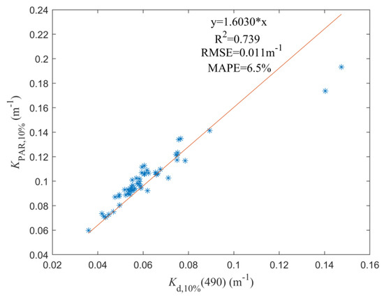
Figure 11.
Relationship between and .
The results obtained with Equation (12) ranged from 5 to 23 m, with an average of approximately 14 m. In particular, the values of at three stations (B1, B2, and Q18) in 2013, which are nearest to the shore, were less than 10 m, and the value of at station S29 in 2015 was greater than 20 m. In order to illustrate the spatial schematic diagram of in the investigation area, ODV was also used the same as in Figure 5, Figure 6 and Figure 7, and the Weighted-average gridding method was used to interpolate the station values. The result is shown in Figure 12.
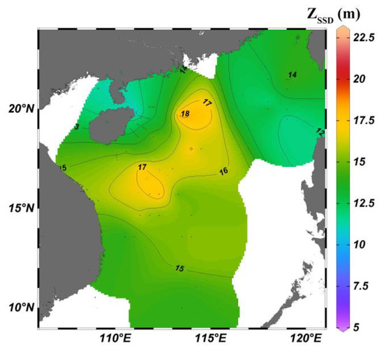
Figure 12.
Spatial diagram of in the investigation area.
4. Discussion
4.1. Discussion about
As demonstrated in Section 3.1 and Section 3.2, presented two significant spectral distributions in the northwestern South China Sea according to Jerlov’s classification; one is more in line with type III, and the other is more like type ΙB and type II. The reason for this difference is that the waters of the northwestern South China Sea are complex and belong to a mixed water where multiple types coexist, and the optical properties are more intricate [31]. As an example, the value of can change from 0.03 to 0.14 with the investigated stations. Owing to diverse human and physical activities, the water at nearshore stations is more turbid than offshore stations, thereby causing a greater value and more significant variation of influenced by water constituents.
Regarding the vertical and horizontal distribution characteristics of in eastern Hainan Island, these vertical and transverse distribution features of , which exhibited an overall decreasing trend from west to east, were found to be consistent with the distribution trends of the temperature and salinity in these longitudinal sections, namely, a significantly low temperature and high salinity were found along the western sea transects [53]. Wang et al. [53] had demonstrated the existence of upwelling on the east coast of Hainan Island during the cruise, so the upwelling process may be responsible for this vertical and horizontal distribution of . Additionally, in section c, the depths of the vertical profile maximum of at stations Q23 and Q24 showed a more significant uplift relative to adjacent stations (as shown in Figure 6c), which is consistent with the uplift contours of the temperature and salinity in this section [53]. The reason for this trend may be that these stations are close to the Pearl River Mouth basin, the seabed topography is complicated and undulating, and there is an upwelling occurring in the shelf slope break zone [54]. Additionally, there was a difference at station Q6 in section d, and significantly increased at a depth of 70 m in section d because of the small station depth (70 m occurs near the seabed), while significant scattering occurred due to the sediment on the seabed.
To investigate the reason for the vertical and horizontal distribution of in eastern Vietnam, the distribution of temperature, salinity, and Chla in sections e, f, and g were compared with . Taking section f as an example, Figure 7 shows a comparative result similar to the region of eastern Hainan Island, where the distribution of was significantly associated with the distribution trend of the temperature, salinity, and Chla. Considering that upwelling is often formed in the region of eastern Vietnam in summer [55] and the vertical distribution of nutrients and the bio-optical properties of water are greatly affected by water mixing [56], the internal reason for the observed convex distribution characteristic in section f might include the contribution of low-temperature and high-salinity upwelling to the promotion of the transport of nutrients from the bottom layer to the upper layer, triggering of phytoplankton growth, and increase in the Chla concentration.
4.2. Comparison of
, calculated by HL60 and the model of Lee (2005) [2] has been compared. In the model of Lee (2005), several model parameters of the solar zenith angles at , , and and several profile depth ranges were determined to calculate . There are three stations (stations Q20 in 2013, Q47 in 2013, and D22 in 2015) with a solar zenith angle at around () and five stations (stations Q6 in 2013, Q34 in 2013, Q45 in 2013, Q48 in 2013, and D10 in 2015) with a solar zenith angle at around () that can be matched for comparison. in 0–20 m profiles obtained from HL60 simulations and the model of Lee (2005) are shown in Figure 13. As shown in Figure 13, there was a suitable agreement between the results obtained from HL60 simulations and the model of Lee (2005). In all stations, the , RMSE, and MAPE were 0.891, 0.004 , and 5.4%, respectively, and there was a better accuracy at all stations with = 0.960, RMSE = 0.001 , and MAPE = 2.1%. Among all these stations with a solar zenith angle at around () and (), calculated by the HL60 and the model of Lee (2005) had an excellent accuracy, with = 0.921, RMSE = 0.003 , and MAPE = 3.3%.
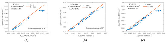
Figure 13.
Comparisons of calculated by HL60 and the model of Lee (2005): (a) stations with a solar zenith angle at around (); (b) stations with a solar zenith angle at around (); (c) stations with a solar zenith angle at around () and ().
Although an excellent agreement has been shown in Figure 13, there is also a subtle difference between the simulations and the model of Lee (2005), and the main factors contributing to this difference are: (1) meteorological parameters; (2) particle phase function; (3) error of Lee’s model itself. Firstly, the values of the model parameters were conducted by Lee et al. [2] based on Hydrolight simulations under clear sky conditions and a wind speed of 5 m/s, while the meteorological parameters input into HL60 in our study were not constant. For example, the wind speed input into HL60 for stations S66 and B1 were 11 and 2.2 . The secondary reason for the difference was the particle phase function. The values of the model parameters in Lee (2005) were conducted following the averaged particle phase function, while the Fournier–Forand phase function was used in this study. The major factor for the discrepancy was that the model parameters conducted by Lee et al. [2] are functions of the profile depth, but in fact the constant was used in the driving process, and this meant that has an error due to the constant parameters, just as Lee et al. [2] mentioned (the average error is between modeled and Hydrolight determined ).
4.3. Comparison of
Lee et al. [4] established an empirical equation for seawater transparency calculation based on (Equation (13)), namely the method of Lee (2018) employed in our study.
where is taken as a constant 1.48 in the study.
The calculated by the method of Lee (2018) and the algorithm for estimation based on has been compared in this study. The average values of were calculated between the surface and the depth where 10% of the PAR(0) [4] was used to represent the on Equation (13). As shown in Figure 14, there was a suitable agreement between the results obtained with the two methods with slope = 0.972, = 0.804, RMSE = 1.326 , and MAPE = 8.9%. The uncertainty in the algorithm for estimation based on was mainly caused by the following: One is in Equation (10); in Equation (10) represents at the euphotic zone depth, while was calculated between the surface and the depth where 10% of PAR(0) was used in this study, and this approximation may generate some errors. The other uncertainty source is the proportionality factor of in Equation (11). Equation (11) is an empirical relationship between and , developed based on field measurements. The proportionality factor, , is not a constant reported in a range of [4,57,58]. The value of taken as a constant 3.5 in this study may introduce some errors to the estimation of based on .
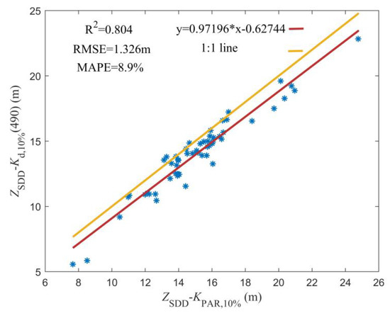
Figure 14.
Comparisons of the calculated values between the two methods.
5. Conclusions
In this study, we simulated the diffuse attenuation coefficient for the downwelling irradiance, , with HL60 based on measured vertical profiles of the IOPs from 9 August to 2 September 2013, and 30 June to 17 July 2015, in the northwestern South China Sea at 55 stations. The results between the simulations and the model of Lee (2005) had an excellent accuracy. The simulation results revealed significant spectral distribution characteristics, with a minimum at approximately 490 nm and a maximum at 670 nm. The spectral characteristics of the simulated values were similar to the spectra of several oceanic types reported by Jerlov [44].
The distribution characteristics of in sections a–d in the eastern Hainan Island area showed an overall decreasing trend from west to east at the same depth, which was significantly associated with the distribution trend of the temperature and salinity. in sections e–g in eastern Vietnam revealed unique horizontal and vertical distribution characteristics, which was completely consistent with the investigated vertical distribution characteristics of the temperature and salinity at the same time. During these cruises, attained a global maximum of approximately 0.14 and a global minimum of 0.035 .
The regression results indicated a satisfactory linear relationship between and from with > 0.76, RMSE 0.010 , and MAPE < 9%, and this result indicated that from could be estimated by , and the closer to 490 nm, the higher and the smaller RMSE and MAPE were between and . This conclusion is consistent with the results reported by Austin et al. [45]. It was also found that the regression slope,, and intercept,, of and from 420~580 nm can be expressed as a quadratic function of the wavelength,, with values of 0.9995 and 0.991, respectively.
Based on the simulations, a linear relationship between and for the northwestern South China Sea was first constructed, and an empirical relationship for estimation based on was then developed, and at all 55 stations was calculated, with a range of 5–23 m and an average of approximately 14 m. calculated in this study suitably agrees with the results obtained via the method of Lee (2018), with a slope of 0.972 and , RMSE, and MAPE values of 0.804, 1.326 , and 8.9%, respectively.
Author Contributions
All authors conceived and designed the study. Conceptualization, X.Z. and C.L. (Cai Li); writing—original draft preparation, X.Z.; writing—review and editing, X.Z. and C.L. (Cai Li); methodology, C.L. (Cai Li), W.Z. and W.C.; investigation, Y.Z., W.Z., C.L. (Cong Liu), Z.X., Y.Y., Z.Y. and F.C.; software, X.Z. and W.Z.; funding acquisition, C.L. (Cai Li), W.C., W.Z., Y.Y. and Z.X. All authors have read and agreed to the published version of the manuscript.
Funding
This research was funded by the National Natural Science Foundation of China (No. 41976181; No. 41976170; No. 41976172); the Scientific and Technological Planning Project of Guangzhou City (201707020023), the State Key Laboratory of Tropical Oceanography, South China Sea Institute of Oceanology, Chinese Academy of Sciences (LTOZZ2003).
Data Availability Statement
All data are available on request.
Acknowledgments
We thank the ODV software (https://odv.awi.de, accessed on 9 March 2022.) for the convenience in drawing.
Conflicts of Interest
The authors declare no conflict of interest.
Abbreviations
The main abbreviations used in this study.
| Abbreviations | Definitions | Units |
| The downwelling irradiance | ||
| The diffuse attenuation coefficient for downwelling irradiance | ||
| Remote sensing reflectance | ||
| Photosynthetically available radiation | ||
| Absorption coefficient | ||
| Attenuation coefficient | ||
| Total minus water absorption coefficient | ||
| Total minus water attenuation coefficient | ||
| Particulate scattering coefficient | ||
| Particulate backscattering coefficient | ||
| Volume scattering function | ||
| Particulate volume scattering function | ||
| Water volume scattering function | ||
| Chlorophyll a concentration | ||
| The absorption of the baseline | ||
| The absorption line height | ||
| based on the absorption line height method | ||
| The Secchi disk depth | ||
| The depth of the euphotic zone | ||
References
- Gordon, H.R.; Smith, R.C.; Ronald, J.; Zaneveld, V. Introduction to Ocean Optics. In Proceedings of the Society of Photo-Optical Instrumentation Engineers (SPIE) Conference Series, Monterey, CA, USA, 1 March 1980; pp. 14–55. [Google Scholar]
- Lee, Z.P.; Du, K.P.; Arnone, R. A model for the diffuse attenuation coefficient of downwelling irradiance. J. Geophys. Res.-Oceans 2005, 110, 10. [Google Scholar] [CrossRef]
- Huang, C.C.; Yao, L.; Huang, T.; Zhang, M.L.; Zhu, A.X.; Yang, H. Wind and rainfall regulation of the diffuse attenuation coefficient in large, shallow lakes from long-term MODIS observations using a semianalytical model. J. Geophys. Res. Atmos. 2017, 122, 6748–6763. [Google Scholar] [CrossRef]
- Lee, Z.P.; Shang, S.L.; Du, K.P.; Wei, J.W. Resolving the long-standing puzzles about the observed Secchi depth relationships. Limnol. Oceanogr. 2018, 63, 2321–2336. [Google Scholar] [CrossRef]
- Enaganti, P.K.; Dwivedi, P.K.; Srivastava, A.K.; Goel, S. Study of solar irradiance and performance analysis of submerged monocrystalline and polycrystalline solar cells. Prog. Photovolt. 2020, 28, 725–735. [Google Scholar] [CrossRef]
- Lewis, M.R.; Carr, M.-E.; Feldman, G.C.; Esaias, W.; McClain, C. Influence of penetrating solar radiation on the heat budget of the equatorial Pacific Ocean. Nature 1990, 347, 543–545. [Google Scholar] [CrossRef]
- Castillo-Ramirez, A.; Santamaria-del-Angel, E.; Gonzalez-Silvera, A.; Frouin, R.; Sebastia-Frasquet, M.T.; Tan, J.; Lopez-Calderon, J.; Sanchez-Velasco, L.; Enriquez-Paredes, L. A New Algorithm to Estimate Diffuse Attenuation Coefficient from Secchi Disk Depth. J. Mar. Sci. Eng. 2020, 8, 558. [Google Scholar] [CrossRef]
- Lee, Z.P.; Darecki, M.; Carder, K.L.; Davis, C.O.; Stramski, D.; Rhea, W.J. Diffuse attenuation coefficient of downwelling irradiance: An evaluation of remote sensing methods. J. Geophys. Res.-Oceans 2005, 110, 9. [Google Scholar] [CrossRef]
- Chen, B.Z.; Wang, L.; Song, S.Q.; Huang, B.Q.; Sun, J.; Liu, H.B. Comparisons of picophytoplankton abundance, size, and fluorescence between summer and winter in northern South China Sea. Cont. Shelf Res. 2011, 31, 1527–1540. [Google Scholar] [CrossRef]
- Zheng, W.; Zhou, W.; Cao, W.; Liu, Y.; Wang, G.; Deng, L.; Li, C.; Zhang, Y.; Zeng, K. Vertical Variability of Total and Size-Partitioned Phytoplankton Carbon in the South China Sea. Remote Sens. 2021, 13, 993. [Google Scholar] [CrossRef]
- Xue, H.J.; Chai, F.; Pettigrew, N.; Xu, D.Y.; Shi, M.; Xu, J.P. Kuroshio intrusion and the circulation in the South China Sea. J. Geophys. Res.-Oceans 2004, 109, 14. [Google Scholar] [CrossRef]
- Wang, M.; And, S.H.S.; Harding, L.W. Retrieval of diffuse attenuation coefficient in the Chesapeake Bay and turbid ocean regions for satellite ocean color applications. J. Geophys. Res. Oceans 2009, 114, C10011. [Google Scholar] [CrossRef]
- Siegel, D.A.; Dickey, T.D. Observations of the Vertical Structure of the Diffuse Attenuation Coefficient Spectrum. Deep-Sea Res. Part A-Oceanogr. Res. Pap. 1987, 34, 547–563. [Google Scholar] [CrossRef]
- Cao, W.X.; Wu, T.F.; Yang, Y.Z.; Ke, T.; Li, C.; Guo, C. Monte Carlo simulations of the optical buoy’s shading effects. High Technol. Lett 2003, 13, 80–84. [Google Scholar]
- Maciel, D.A.; Barbosa, C.C.F.; de Moraes Novo, E.M.L.; Cherukuru, N.; Martins, V.S.; Júnior, R.F.; Jorge, D.S.; de Carvalho, L.A.S.; Carlos, F.M. Mapping of diffuse attenuation coefficient in optically complex waters of amazon floodplain lakes. ISPRS-J. Photogramm. Remote Sens. 2020, 170, 72–87. [Google Scholar] [CrossRef]
- Qing, S.; Cui, T.W.; Tang, J.W.; Song, Q.J.; Liu, R.J.; Bao, Y.H. An optical water classification and quality control model (OC_QC model) for spectral diffuse attenuation coefficient. ISPRS-J. Photogramm. Remote Sens. 2022, 189, 255–271. [Google Scholar] [CrossRef]
- Austin, R.W.; Petzold, T.J. The Determination of the Diffuse Attenuation Coefficient of Sea Water Using the Coastal Zone Color Scanner. In Oceanography from Space; Springer: Boston, MA, USA, 1981. [Google Scholar]
- Mueller, J.L. SeaWiFS algorithm for the diffuse attenuation coefficient, K (490), using water-leaving radiances at 490 and 555 nm. SeaWiFS Postlaunch Calibration Valid. Anal. 2000, 3, 24–27. [Google Scholar]
- Tiwari, S.P.; Shanmugam, P. A Robust Algorithm to Determine Diffuse Attenuation Coefficient of Downwelling Irradiance From Satellite Data in Coastal Oceanic Waters. IEEE J. Sel. Top. Appl. Earth Observ. Remote Sens. 2014, 7, 1616–1622. [Google Scholar] [CrossRef]
- Zhang, T.; Fell, F. An empirical algorithm for determining the diffuse attenuation coefficient Kd in clear and turbid waters from spectral remote sensing reflectance. Limnol. Oceanogr. Methods 2007, 5, 457–462. [Google Scholar] [CrossRef]
- Zhang, Y.; Wang, G.; Xu, Z.; Yang, Y.; Zhou, W.; Zheng, W.; Zeng, K.; Deng, L. Retrieval of diffuse attenuation coefficient in high frequency red tide area of the East China Sea based on buoy observation. J. Trop. Oceanogr. 2020, 39, 71–83. [Google Scholar]
- Preisendorfer, R.W. Hydrologic Optics; US Department of Commerce, National Oceanic and Atmospheric Administration: Washington, DC, USA, 1976.
- Kirk, J.T.O. Monte-Carlo Study of the Nature of the Underwater Light-Field in, and the Relationships between Optical-Properties of, Turbid Yellow Waters. Aust. J. Mar. Freshw. Res. 1981, 32, 517–532. [Google Scholar] [CrossRef]
- Gordon, H.R. Can the Lambert-Beer law be applied to the diffuse coefficient of ocean water? Limnol. Oceanogr. 1989, 34, 1389. [Google Scholar] [CrossRef]
- Kirk, J.T.O. Estimation of the Absorption and the Scattering Coefficients of Natural-Waters by Use of Underwater Irradiance Measurements. Appl. Opt. 1994, 33, 3276–3278. [Google Scholar] [CrossRef] [PubMed]
- Mobley, C.D. Light and Water: Radiative Transfer in Natural Waters; Academic Press: Cambridge, MA, USA, 1994. [Google Scholar]
- He, S.Y.; Zhang, X.D.; Xiong, Y.H.; Gray, D. A Bidirectional Subsurface Remote Sensing Reflectance Model Explicitly Accounting for Particle Backscattering Shapes. J. Geophys. Res.-Oceans 2017, 122, 8614–8626. [Google Scholar] [CrossRef]
- Mobley, C.D.; Sundman, L.K.; Boss, E. Phase function effects on oceanic light fields. Appl. Opt. 2002, 41, 1035–1050. [Google Scholar] [CrossRef]
- Huang, J.; Duan, H.; Ma, R.; Zhang, Y. Study on regional parameters of radiative transfer simulation based on Hydrolight in Taihu Lake. J. Univ. Chin. Acad. Sci. 2014, 31, 613–625. [Google Scholar]
- Liu, Q.; Liu, B.Y.; Wu, S.H.; Liu, J.T.; Zhang, K.L.; Song, X.Q.; Chen, X.C.; Zhu, P.Z. Design of the Ship-Borne Multi-Wavelength Polarization Ocean Lidar System and Measurement of Seawater Optical Properties. In Proceedings of the 29th International Laser Radar Conference (ILRC), Hefei, China, 24–28 June 2019. [Google Scholar]
- Wang, G.F.; Cao, W.X.; Yang, D.T.; Xu, D.Z. Variation in downwelling diffuse attenuation coefficient in the northern South China Sea. Chin. J. Oceanol. Limnol. 2008, 26, 323–333. [Google Scholar] [CrossRef]
- Zhao, W.; Cao, W.; Hu, S.; Wang, G. Comparison of diffuse attenuation coefficient of downwelling irradiance products derived from MODIS-Aqua in the South China Sea. Opt. Precis. Eng. 2018, 26, 14–24. [Google Scholar] [CrossRef]
- Saulquin, B.; Hamdi, A.; Gohin, F.; Populus, J.; Mangin, A.; d’Andon, O.F. Estimation of the diffuse attenuation coefficient KdPAR using MERIS and application to seabed habitat mapping. Remote Sens. Environ. 2013, 128, 224–233. [Google Scholar] [CrossRef]
- Zaneveld, J.R.V.; Bartz, R.; Kitchen, J.C. Reflective-tube absorption meter. In Proceedings of the Ocean Optics X, Orlando, FL, USA, 16–18 April 1990; pp. 124–136. [Google Scholar]
- Maffione, R.A.; Dana, D.R. Instruments and methods for measuring the backward-scattering coefficient of ocean waters. Appl. Opt. 1997, 36, 6057–6067. [Google Scholar] [CrossRef]
- Pope, R.M.; Fry, E.S. Absorption spectrum (380–700 nm) of pure water. 2. Integrating cavity measurements. Appl. Opt. 1997, 36, 8710–8723. [Google Scholar] [CrossRef]
- Sullivan, J.M.; Twardowski, M.S.; Zaneveld, J.R.V.; Moore, C.M.; Barnard, A.H.; Donaghay, P.L.; Rhoades, B. Hyperspectral temperature and salt dependencies of absorption by water and heavy water in the 400–750 nm spectral range. Appl. Opt. 2006, 45, 5294–5309. [Google Scholar] [CrossRef]
- Zaneveld, J.R.; Kitchen, J.; Moore, C. Scattering Error Correction of Reflection-Tube Absorption Meters. In Proceedings of the SPIE, Rome, Italy, 26–30 September 1994; Volume 2258. [Google Scholar]
- Savitzky, A.; Golay, M.J. Smoothing and differentiation of data by simplified least squares procedures. Anal. Chem. 1964, 36, 1627–1639. [Google Scholar] [CrossRef]
- Zhang, X.D.; Hu, L.B.; He, M.X. Scattering by pure seawater: Effect of salinity. Opt. Express 2009, 17, 5698–5710. [Google Scholar] [CrossRef]
- Boss, E.; Picheral, M.; Leeuw, T.; Chase, A.; Karsenti, E.; Gorsky, G.; Taylor, L.; Slade, W.; Ras, J.; Claustre, H. The characteristics of particulate absorption, scattering and attenuation coefficients in the surface ocean; Contribution of the Tara Oceans expedition. Methods Oceanogr. 2013, 7, 52–62. [Google Scholar] [CrossRef]
- Roesler, C.S.; Barnard, A.H. Optical proxy for phytoplankton biomass in the absence of photophysiology: Rethinking the absorption line height. Methods Oceanogr. 2013, 7, 79–94. [Google Scholar] [CrossRef]
- Deng, L.; Zhou, W.; Cao, W.; Zheng, W.; Wang, G.; Xu, Z.; Li, C.; Yang, Y.; Hu, S.; Zhao, W. Retrieving phytoplankton size class from the absorption coefficient and chlorophyll a concentration based on support vector machine. Remote Sens. 2019, 11, 1054. [Google Scholar] [CrossRef]
- Jerlov, N.G. Marine Optics; Elsevier: Amsterdam, The Netherlands, 1976. [Google Scholar]
- Austin, R.W. Spectral Dependence Of The Diffuse Attenuation Coefficient Of Light In Ocean Waters. Opt. Eng. 1986, 25, 253471. [Google Scholar] [CrossRef]
- Choubey, V.K. Laboratory experiment, field and remotely sensed data analysis for the assessment of suspended solids concentration and secchi depth of the reservoir surface water. Int. J. Remote Sens. 1998, 19, 3349–3360. [Google Scholar] [CrossRef]
- McQueen, D.J.; Johannes, M.R.S.; Lafontaine, N.R.; Young, A.S.; Longbotham, E.; Lean, D.R.S. Effects of Planktivore Abundance on Chlorophyll-A and Secchi Depth. Hydrobiologia 1990, 200, 337–341. [Google Scholar] [CrossRef]
- Civera, J.I.; Breijo, E.G.; Miro, N.L.; Sanchez, L.G.; Baixauli, J.G.; Gil, I.R.; Peris, R.M.; Fillol, M.A. Artificial neural network onto eight bit microcontroller for Secchi depth calculation. Sens. Actuator B-Chem. 2011, 156, 132–139. [Google Scholar] [CrossRef]
- Preisendorfer, R.W. Secchi Disk Science—Visual Optics of Natural-Waters. Limnol. Oceanogr. 1986, 31, 909–926. [Google Scholar] [CrossRef]
- Lee, Z.P.; Shang, S.L.; Hu, C.M.; Du, K.P.; Weidemann, A.; Hou, W.L.; Lin, J.F.; Lin, G. Secchi disk depth: A new theory and mechanistic model for underwater visibility. Remote Sens. Environ. 2015, 169, 139–149. [Google Scholar] [CrossRef]
- Platt, T. Primary production of the ocean water column as a function of surface light intensity: Algorithms for remote sensing. Deep Sea Res. Part A. Oceanogr. Res. Pap. 1986, 33, 149–163. [Google Scholar] [CrossRef]
- Austin, R.W.; Petzold, T.J. Spectral dependence of the diffuse attenuation coefficient of light in ocean waters: A reexamination using new data. In Proceedings of the Ocean Optics X, Orlando, FL, USA, 16–18 April 1990; pp. 79–93. [Google Scholar]
- Wang, Y.; Jing, Z.; Qi, Y. Coastal upwelling off eastern Hainan Island observed in the summer of 2013. J. Trop. Oceanogr. 2016, 35, 40–49. [Google Scholar]
- Chen, H.; Zhan, W.; Wen, M.; Li, L. Characteristics of shelf break and sedimentaion process at the Qiongdongnan basin, Northwestern South China Sea. Mar. Geol. Front. 2015, 31, 1–9. [Google Scholar]
- Wu, R.S.; Li, L. Summarization of study on upwelling system in the South China Sea. J. Oceanogr. Taiwan Strait 2003, 22, 269–276. [Google Scholar]
- Huang, B.Q.; Han, Z.M.; Cheng, X.R.; Wang, P.X. Foraminiferal responses to upwelling variations in the South China Sea over the last 220,000 years. Mar. Micropaleontol. 2003, 47, 1–15. [Google Scholar] [CrossRef]
- Koenings, J.; Edmundson, J. Secchi disk and photometer estimates of light regimes in Alaskan lakes: Effects of yellow color and turbidity. Limnol. Oceanogr. 1991, 36, 91–105. [Google Scholar] [CrossRef]
- Luhtala, H.; Tolvanen, H. Optimizing the use of Secchi depth as a proxy for euphotic depth in coastal waters: An empirical study from the Baltic Sea. ISPRS Int. J. Geo-Inf. 2013, 2, 1153–1168. [Google Scholar] [CrossRef]


Disclaimer/Publisher’s Note: The statements, opinions and data contained in all publications are solely those of the individual author(s) and contributor(s) and not of MDPI and/or the editor(s). MDPI and/or the editor(s) disclaim responsibility for any injury to people or property resulting from any ideas, methods, instructions or products referred to in the content. |
© 2023 by the authors. Licensee MDPI, Basel, Switzerland. This article is an open access article distributed under the terms and conditions of the Creative Commons Attribution (CC BY) license (https://creativecommons.org/licenses/by/4.0/).