Mutual Information Boosted Precipitation Nowcasting from Radar Images

Abstract

Precipitation nowcasting has long been a challenging problem in meteorology. While recent studies have introduced deep neural networks into this area and achieved promising results, these models still struggle with the rapid evolution of rainfall and extremely imbalanced data distribution, resulting in poor forecasting performance for convective scenarios. In this article, we evaluate the amount of information in different precipitation nowcasting tasks of varying lengths using mutual information. We propose two strategies: the mutual information-based reweighting strategy (MIR) and a mutual information-based training strategy (time superimposing strategy (TSS)). MIR reinforces neural network models to improve the forecasting accuracy for convective scenarios while maintaining prediction performance for rainless scenarios and overall nowcasting image quality. The TSS strategy enhances the model’s forecasting performance by adopting a curriculum learning-like method. Although the proposed strategies are simple, the experimental results show that they are effective and can be applied to various state-of-the-art models.

1. Introduction

Precipitation nowcasting aims to predict the kilometer-wise rainfall intensity within the next two hours [1]. It plays a vital role in daily life, such as traffic planning, disaster alerts, and agriculture [2]. Precipitation nowcasting is often defined as a spatiotemporal sequence prediction task [3,4,5,6,7]. A sequence of historical radar echo images is taken in and a sequence of future radar echo images is predicted [3]. In this paper, we denote the historical radar echo images as X and the future (to be predicted) radar echo images as Y. The rainfall intensity distribution of the whole dataset will be $P\left(Y\right)$ (or $P\left(X\right)$, because both X and Y are drawn from the same distribution), and the precipitation nowcasting task can be represented as $P\left(Y\right|X)$.

However, due to the highly skewed distribution of rainfall intensities, the traditional approach has a limited ability to forecast heavy rainfall scenarios [8]. For instance, using the Italian dataset TAASRAD19 [9] as an example, the number of pixels with a radar reflective intensity greater than 50 dBZ accounts for only 0.066% of the total number of pixels, and only 0.45% of pixels are greater than 40 dBZ. The same situation also exists in the ECP dataset [10] and HKO-7 dataset [11], as illustrated in Figure 1. Radar echo intensity (dBZ) does not correspond to the rainfall intensity (mm/h). The conversion from radar reflectivity to rainfall intensity requires a precipitation estimation algorithm, such as the Z–R relation formula. This paper focuses on radar echo intensity prediction; rainfall intensity can be estimated from the predicted radar echo intensity using an estimation algorithm [3].

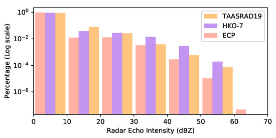
Figure 1. Distribution of different radar echo intensity levels. ECP and TAASRAD19 were collected from the north temperate zone, and HKO-7 was collected from the tropics.

Heavy rainfall scenarios are often rare; however, if left unaddressed, they will have more severe consequences than moderate to light rainfall scenarios. Therefore, efforts have been devoted to improving the heavy rain forecasting performance, with reweighting and resampling being the most popular strategies [8,11,12]. These strategies could increase the heavy rainfall sample weights based on $P\left(Y\right)$.

However, adjusting the sample weights or prediction losses based on $P\left(Y\right)$ would undermine the conditional distribution $P\left(Y\right|X)$, downgrading the majority classes’ performance and hurting the overall rainfall prediction accuracy.

In this work, we propose a new strategy, mutual-information-based reweighting (MIR), to improve the nowcasting prediction for imbalanced rainfall data. Mutual information $I(X;Y)$ measures the dependence between random variables X and Y, with high mutual information corresponding to high-dependency X and Y (easy-to-learn) tasks, and low mutual information corresponding to low-dependency (hard-to-learn) tasks [13].

In the task of precipitation nowcasting, we calculate the mutual information of the radar echo data and observe that tasks with more mutual information exhibit greater resilience to the issue of data imbalance. Specifically, when the mutual information is high, MIR employs relatively mild reweighting factors to preserve the original distribution of $P\left(Y\right|X)$. Conversely, for tasks with low mutual information, MIR employs higher reweighting factors to enhance the prediction performance. This approach boosts the performance of the minority groups without negatively impacting the overall prediction performance.

Furthermore, we propose a simple curriculum-style training strategy, the time superimposing strategy (TSS). The primary advantage of curriculum learning is that it enables machines to start learning with more manageable tasks and gradually progress to more challenging ones. Inspired by this, TSS first trains the model with the highest mutual information task and gradually stacks the lower mutual information tasks into the training task set. Regarding implementation, the TSS strategy only requires control over the forecast time length during loss calculation during the training phase, which can be achieved by adding just one or two lines of code.

This work is an extension of our previous work [14], which fused MIR and TSS together. In this paper, we elaborate on the MIR and TSS strategies separately, provide a more detailed experimental analysis, and extensively discuss different aspects of the proposed strategies.

The remainder of this paper is organized as follows. Section 2 briefly reviews the related works about deep learning models and the data imbalance problem in precipitation nowcasting. In Section 3, we describe how to compute the mutual information for the precipitation nowcasting task. Then, a reweighting strategy, MIR (Section 3.2), and a curriculum-learning-style training strategy, TSS (Section 3.3), are proposed based on the mutual information of the training tasks. Extensive experiments in Section 4 reveal that the proposed MIR and TSS strategies reinforce the state-of-the-art models’ performances using a large gap without downgrading the overall prediction performance. Section 5 discusses several research questions. The conclusions are shown in Section 6.

2. Related Works

2.1. Models for Precipitation Nowcasting

Precipitation nowcasting models can be classified into three categories: numerical weather prediction methods, extrapolation-based methods, and deep-learning-based end-to-end methods [10]. This paper concentrates on the latter due to their exceptional performance. To be more specific, deep learning models can be categorized into two types: ConvLSTM-based and UNet-based models [15].

The ConvLSTM proposed by Shi et al. is a notable achievement in this field. This replaces the fully connected layer in the long short-term memory (LSTM) [16] with a convolution layer and extends LSTM to the image domain. Subsequently, many ConvLSTM-based models emerged [17]. For example, in TrajGRU [11], the convolution layer was transformed into a non-local version and analogically integrated with GRUs to allow for the active learning of location-variant patterns. PredRNN, introduced by Wang et al. [18], separates the spatial and temporal memory and communicates them at distinct LSTM levels. Another model by Espeholt et al. [19] uses a ConvLSTM-based approach for large-scale precipitation forecasting, which is capable of predicting up to 12 hours in advance.

Nowcasting models based on UNet [20], such as RainNet [21], vanilla UNet [22], and MSST-Net [23], have recently emerged, thanks to the faster training capability of CNN compared to RNN. Agrawa et al. [22] treated forecasting as an image-to-image translation, and thus adopted UNet to classify at a high resolution in terms of both space and intensity, which was similar to the SmaAt-UNet [24] approach. Moreover, they equipped the basic UNet with the attention modules and achieved competitive accuracy, notably reducing the number of trainable parameters. T-UNet [25] combines TrajGRU and UNet to further improve the model’s forecasting ability.

Furthermore, GAN was adopted in the precipitation nowcasting tasks to improve the imagery quality [26]. DGMR, proposed by Ravuri et al. [12], adopts a UNet encoder and a ConvLSTM decoder to solve the blurry problem from the perspective of generative models. These models improve the nowcasting performance compared to the original ConvLSTM model by modifying the network structure to enhance the fitting ability. We argue that fitting ability is not the only key factor in this task. Rethinking the nowcasting problem in the task from a data perspective helped us to acquire better nowcasting models in this paper.

2.2. Data Imbalance

The data imbalance problem is prevalent in various forms of natural data [27]. The research on data imbalance has a long history and generally refers to the problem where the uneven distribution of $P\left(Y\right)$ affects the model training. The basic assumption is that the $P\left(Y\right)$ of the training data is unbalanced, making it easy for the model to train trivial solutions, which leads to a good performance in the majority class and poor performance in the minority class [28]. In Section 3.2, we challenge this assumption using a toy classification problem.

Resampling and reweighting are two common strategies for addressing the data imbalance problem. The typical strategy is over-sampling or up-weighting minority classes [29]. However, in precipitation nowcasting, the resampling method is usually performed patch-wise or sample-wise, which is less feasible for the pixel-level imbalanced precipitation data [8]. Reweighting methods are proposed to adjust the importance of different rainfall intensity samples to balance the impact of data imbalance using the reweighted loss for different rainfall intensities [8,11]. Ravuri et al. [12] adopted the importance of sampling and reweighting to reduce the number of rainless samples. Although these works improve the forecast indicators for the minority class (heavy rainfall), they compromise the model performance on the majority class and the overall image quality.

There are other ways to mitigate the data imbalance problem. Feature selection techniques help to pre-process the data [30]. Recent studies also indicated that semi-supervised and self-supervised learning strategies alleviate the influence of imbalanced data [31]. In contrast to these works, we rethink the data imbalance assumption and analyze the data imbalance problem by considering mutual information.

3. Methodology

In this section, we begin by explaining the process of calculating conditional distribution and mutual information, which is essential when identifying tasks with a high or low information content. Next, we explore the connection between mutual information and the data imbalance problem, and present a novel mutual information-based reweighting approach that addresses the limitations of existing methods. Finally, we introduce a curriculum-style learning strategy that guides the model to learn tasks progressively. This approach prioritizes tasks with a high level of mutual information, allowing for the model to master them before moving on to those with lower mutual information.

3.1. Estimating the Mutual Information on Precipitation Nowcasting Tasks

Existing deep-learning-based models [10,11,18] usually regard the precipitation nowcasting task as a spatiotemporal forecasting problem. Models encode information from a sequence of $n+1$ historical radar echo images and generate a sequence of m future radar echo images that are most likely to occur, which can be formulated as

$$\begin{array}{c}\hfill {\widehat{\mathcal{S}}}_{n:n+m-1}=\underset{{\mathcal{S}}_{n:n+m-1}}{arg\; max}p\left({\mathcal{S}}_{n:n+m-1}\right|{\mathcal{S}}_{0:n-1}),\end{array}$$

(1)

where $\mathcal{S}\in {\mathbb{R}}^{T\times H\times W}$ is the radar echo image sequence, $T=m+n$ is the temporal length, and H and W are the height and the width of images, respectively. Each pixel in the rainfall data has an echo intensity value within $[0-70]\mathrm{dBZ}$, corresponding to the rainfall intensity.

In information theory, the mutual information $I(X;Y)$ is proposed to quantify the information gain achieved by Y by knowing X, and vice versa [13]. This is defined as $I(X;Y):=H\left(Y\right)-H\left(Y\right|X)$, where information entropy $H\left(Y\right):={\sum }_{y}p\left(y\right)log\frac{1}{p\left(y\right)}$ and conditional entropy $H\left(Y\right|X):={\sum }_{x,y}p(x,y)log\frac{1}{p\left(y\right|x)}$. When X and Y are independent, $H\left(Y\right|X)=H(Y)$ and $I(X;Y)=0$; when X determines Y, $I(X;Y)=H\left(Y\right)$.

However, calculating the mutual information in a high-dimensional task is challenging. Mutual information $I(X;Y)$ measures the dependence between random variables X and Y, which involves an estimate of the probability density distribution $P(X,Y)$ and an estimate of the marginal distributions $P\left(X\right)$ and $P\left(Y\right)$. When the task is low-dimensional, it is relatively easy to obtain sufficient training data to estimate $P(X,Y)$; however, when the task is high-dimensional, it is hard to obtain extensive enough training datasets to estimate $P(X,Y)$. This phenomenon is called the curse of dimensionality. As a result, previous researchers usually train large and over-parameterized generative models with limited training data to approximate $P(X,Y)$.

To avoid training an approximated generative model for $P(X,Y)$ estimation, we transfer the high-dimensional radar echo image intensity prediction task into a one-dimensional radar echo pixel intensity prediction task. More specifically, in this section, we regard the precipitation nowcasting task as a series of pixel prediction tasks with different forecasting lengths. As the dimension of Y shrinks to 1, estimating $P(X,Y)$ and $I(X;Y)$ is straightforward and easy. In this way, mutual information is calculated.

To calculate the joint probability distribution, we first propose redefining the precipitation nowcasting task at the pixel level:

$${\widehat{y}}_{i,t_1}=\underset{y_{i,t_1}}{arg\; max}p\left(y_{i,t_1}\right|x_{i,t_0},{\mathcal{N}}_{i,t_0}),$$

(2)

where $x_{i,t_0}$ denotes the value of the pixel i at time $t_0$, $\mathcal{N}i,t_0$ refers to the set of spatiotemporal neighbors (Here, neighbors of pixel i are the pixels from the length-l cube centered at pixel i) of pixel i at time $t_0$, and $yi,t_1$ represents the value of pixel i at time $t_1$, where $t_1\ge t_0$. It is important to note that $x_{i,t_0}=y_{i,t_0}$. Equations (1) and (2) are equivalent only if ${\mathcal{N}}_{i,t_0}$ covers current as well as all past image pixels.

Next, we employ a three-dimensional Gaussian convolution, $G_{3d}(·)$, of size $l\times l\times l$ on each pixel i to merge the information of spatiotemporal neighboring pixels.

$$x_{i,t_0}^{\prime }=G_{3d}(x_{i,t_0},{\mathcal{N}}_{i,t_0}).$$

(3)

During this procedure, only the first-order spatiotemporal information is kept, and higher-order information such as standard deviation and gradient direction is lost. Then, Equation (2) could be rewritten as:

$${\widehat{y}}_{i,t_1}=\underset{y_{i,t_1}}{arg\; max}p\left(y_{i,t_1}\right|x_{i,t_0}^{\prime }).$$

(4)

Third, we compute the conditional distribution $P\left(Y_{t_1}\right|X_{t_0}^{\prime })$ across the whole training dataset, which approximates $P\left(Y_{t_1}\right|X_{t_0})$. The conditional probability is computed as:

$$\begin{array}{c}\hfill p\left(y\right|x)=\frac{{\sum }_i{\displaystyle \mathbb{𝟙}}(y_{i,t_1}=y\mathrm{and}{x}_{i,t_0}^{\prime }=x)}{{\sum }_i\mathbb{𝟙}(x_{i,t_0}^{\prime }=x)},\mathrm{where}\mathbb{𝟙}\left(c\right)=\left\{\begin{array}{c}0\mathrm{if}c\mathrm{is}\mathrm{False}\hfill \\ 1\mathrm{if}c\mathrm{is}\mathrm{True}\hfill \end{array}\right.\end{array}$$

(5)

Finally, mutual information is computed as:

$$I(X_{t_0}^{\prime };Y_{t_1})=\sum _{y\in Y_{t_1}}\sum _{x\in X_{t_0}^{\prime }}p\left(y\right|x)p\left(x\right){log}_2\left(\frac{p\left(y\right|x)}{p\left(y\right)}\right).$$

(6)

Here, the probability $p\left(y\right)$ and $p\left(x\right)$ can be obtained similarly, as $p\left(y\right|x)$. The mutual information $I(X,Y)$ indicates the degree to which X determines Y; therefore, we can use it to measure the degree to which $X_{t_0}^{\prime }$ determines $Y_{t_1}$.

Figure 2 displays two conditional distribution matrices. To facilitate interpretation, the rainfall intensity is divided into five categories of equal size. The mutual information for the three precipitation nowcasting datasets with different t values is shown in Figure 3, where $t:=t_1-t_0$. It should be noted that the mutual information does not always monotonically decrease with increasing t. For instance, the mutual information fluctuates periodically when dealing with periodic data as t increases.

Figure 2. The conditional distributions $P\left(Y\right|X)$ of two precipitation nowcasting tasks on one dataset. Left: Task predicting future radar echo intensity in the next 10 min. Right: Task predicting future intensity in the next 100 min. The radar echo intensity (0–70 dBZ) is evenly divided into five categories, and the X and Y axes stand for the index of each category. The value in each cell represents the corresponding joint probability $P\left(Y\right|X)$. Take $0.95$ in the bottom-left corner of the left image as an example: if the current intensity is in category 1 (0–14 dBZ), the probability that the intensity in 10 min is still category 1 is $0.95$.

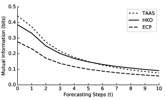
Figure 3. Mutual information of tasks with different forecasting lengths from three precipitation datasets.

3.2. Mutual Information-Based Reweighting (MIR) Strategy

While reweighting methods based on $P\left(Y\right)$ may decrease the quality of generated images, sacrificing part of the majority’s performance to improve the minority is still acceptable in precipitation nowcasting, where heavy rainfall is more critical. This subsection proposes a new reweighting scheme that considers mutual information to adjust the weighting factors. To better understand the relationship between data imbalances and mutual information, consider a binary classification experiment.

3.2.1. Motivating Example

In this experiment, the training data are sampled from two one-dimensional Gaussian distributions A and B, where $\mathrm{A}=\mathcal{N}({\mu }_A,1)$, $\mathrm{B}=\mathcal{N}({\mu }_B,1)$, and $\Delta \mu :=|{\mu }_A-{\mu }_B|$. The objective is to train a binary classifier to distinguish whether a testing sample is generated from A or B. The testing dataset is balanced, and a three-layer, fully connected network is used as the model.

Table 1 displays the mean absolute error (MAE) for different levels of imbalance ratios and $\Delta \mu$ settings. The mutual information values are indicated within the brackets. The model’s prediction is considered correct when the MAE equals to 0, and is regarded as random guessing when the MAE equals 0.5.

Table 1. MAE of the imbalanced binary classification problem. The imbalance ratio refers to the ratio of the number of samples in class A to the number of samples in class B.

Imbalance Ratio	MAE (Mutual Information)
	$\Delta \mathbf{\mu }=\mathbf{20}$	$\Delta \mathbf{\mu }=\mathbf{10}$	$\Delta \mathbf{\mu }=\mathbf{3}$	$\Delta \mathbf{\mu }=\mathbf{1}$	$\Delta \mathbf{\mu }=\mathbf{0.1}$
1:99	0.00 (0.08)	0.00 (0.08)	0.26 (0.06)	0.48 (0.02)	0.50 (0.01)
10:90	0.00 (0.47)	0.00 (0.47)	0.13 (0.35)	0.44 (0.06)	0.50 (0.08)
50:50	0.00 (1.00)	0.00 (1.00)	0.11 (0.74)	0.40 (0.16)	0.50 (0.09)

Traditionally, the data imbalance issue has been associated with the reduced performance of minority classes due to the imbalanced $P\left(Y\right)$. This holds true when $\Delta \mu$ is constant. However, when the imbalance ratio is constant, the MAE decreases as $\Delta \mu$ and mutual information increases, indicating that the impact of data imbalance is reduced. The model becomes resilient to data imbalances when the standard deviation equals one, and $\Delta \mu \ge 10$. This experiment demonstrates that the imbalanced distribution does not necessarily lead to poor performance for the minority class. High mutual information tasks result in better model training when the imbalance ratio is constant compared to low mutual information tasks.

In an imbalanced setting, such as 1:99, the mutual information is lower than in a balanced setting because the information entropy $H\left(Y_{1:99}\right)=0.08$, representing the upper bound of mutual information. Therefore, the trend of mutual information values within each imbalance ratio is more important than the value itself. When the imbalance ratio or $P\left(Y\right)$ is constant, mutual information can help to identify settings that are more resilient to the impact of data imbalance. Thus, it is unnecessary to use reweighting strategies for high mutual information tasks, avoiding the side effect of image quality degradation.

3.2.2. MIR Strategy

Figure 3 shows that mutual information is high for small values of t. Therefore, a rebalancing strategy is unnecessary and could lead to misinformation in $P\left(Y\right|X)$. To address this issue, we propose a reweighting ratio $r_t$, $0<r_t\le 1$ as the exponential factor of the reweighting factor w, based on $P\left(Y\right)$:

$$w_t^{\prime }=w^{r_t},\mathrm{where}{r}_t\propto 1/I(X^{\prime };Y_t),$$

(7)

where w uses the same reweighting factors as WMSE [11]. The new weighting factor $w^{\prime }t$ is directly multiplied by the respective loss to derive the reweighted loss. A simple solution is $rt=t/m$ because mutual information negatively correlates with t. The proposed $w^{\prime }t$ meets the requirement of an unweighted loss at higher mutual information and a precipitous $w^{\prime }t$ for lower mutual information. This approach avoids degrading image quality and undermining the original distribution of reweighting strategies.

In this paper, we adopted the same weighting factor w of $w_t^{\prime }=w^{r_t}$ following the weighted mean square error (WMSE) [11], which is

$$w\left(x_i\right)=\left\{\begin{array}{cc}1,\hfill & x_i<22.4\hfill \\ 2,\hfill & 22.4\le x_i<28.6\hfill \\ 5,\hfill & 28.6\le x_i<33.3\hfill \\ 10,\hfill & 33.3\le x_i<40.7\hfill \\ 30,\hfill & x_i\ge 40.7\hfill \end{array},\mathrm{where}0\le x_i\le 70\mathrm{dBZ}\right.$$

Since the degree to which $I(X_{t_0}^{\prime };Y_{t_1})$ affecting the model’s resistance of data imbalance was unknown, we tried several different naive $r_t$ solutions:

(a)

Linear to t: $r_t=\alpha t+\beta$, where $1\le t\le 10$, $\alpha$ is a constant that controls the expected growing speed of $r_t$. The code is shown in Algorithm 1.

(b)

Exponential: $r_t={\alpha }^{t-m}$, where $\alpha >1$ is a constant that depends on the expected growing speed of $r_t$, and $m=10$ in this paper.

(c)

Linear to $1/I(X^{\prime };Y)$:

$r_t=min\left(I(X_{t_0}^{\prime };Y_{t_1})\right)/I(X_{t_0}^{\prime };Y_{t_1})$. When $t=10$, $min\left(I(X_{t_0}^{\prime };Y_{t_1})\right)=I(X_{t_0}^{\prime };Y_{t_1})$. As shown in Figure 4, this solution is similar to a special version of the linear solution.

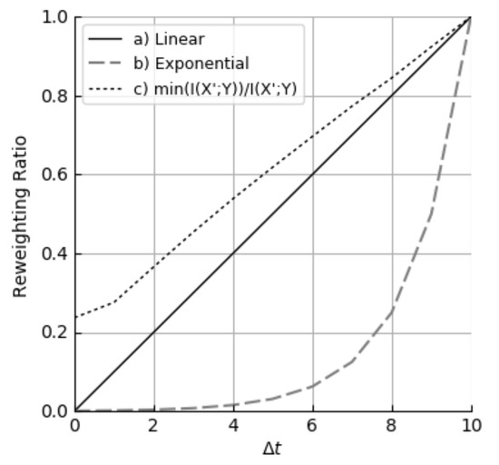Figure 4. Three strategies of MIR.

Algorithm 1 MIR Strategy

Input:  Model $model$, Input Data x, Ground Truth $gt$, WMSE Function $wmse$, Weighting Factor w. Output:  Loss ${\mathcal{L}}_{MIR}$.   1: $pred\leftarrow model\left(x\right)$   2: ${\mathcal{L}}_{MIR}\leftarrow 0$   3: for$t\leftarrow 1to10$do        $▹\mathrm{Forecasting}10\mathrm{Steps}$   4:     $r\leftarrow t/10$          $▹\mathrm{Linear}\mathrm{Solution}$   5:     $w_t^{\prime }\leftarrow w^r$   6:     ${\mathcal{L}}_{MIR}+=wmse(pred\left[t\right],gt\left[t\right],w_t^{\prime })$   7: end for   8: return${\mathcal{L}}_{MIR}$

3.3. Time Superimposing Strategy (TSS)

Traditionally, neural network models are simultaneously trained with all tasks, from $t=1$ to $t=10$. The graph in Figure 3 illustrates that the training task at $t=1$ provides the highest amount of information. As the forecasting length t increases, the mutual information steadily decreases. We adopt a curriculum learning approach to improve training efficiency and reorganize the training order of different forecasting length tasks. A straightforward strategy is to start with high mutual information tasks and gradually move to low mutual information tasks.

Suppose there is a set of training tasks, and the model is trained with all the tasks in the set during every iteration of the training process. The task set starts with only the task for $t=1$, and progressively incorporates other forecasting tasks with increasing lengths until $t=10$.

To be specific, the initial training task is $P\left(Y_{t_1=1}\right|X_{t_0})$. In the next stage, we simultaneously train $P\left(Y_{t_1=1}\right|X_{t_0})$ and $P\left(Y_{t_1=2}\right|X_{t_0})$. In stage three, we simultaneously train $P\left(Y_{t_1=1}\right|X_{t_0})$, $P\left(Y_{t_1=2}\right|X_{t_0})$, and $P\left(Y_{t_1=3}\right|X_{t_0})$, and so on.

We name this method the time superimposing strategy (TSS). TSS could be simplified into a loss function controlling forecasting length. The TSS with fixed training iterations per stage is shown in Algorithm 2. More TSS variants are discussed in Section 4.3.

Algorithm 2 TSS Strategy

Input:  Total Iteration $iter$, Iteration Per Stage L, Model’s Output $pred$, Ground Truth $gt$, Loss Function $\mathcal{L}(·,·)$. Output:  Loss ${\mathcal{L}}_{TSS}$.   1: $t\leftarrow *\frac{iter}{L}$   2: ${\mathcal{L}}_{TSS}\leftarrow \mathcal{L}(pred[0:t],gt[0:t])\hspace{1em}\hspace{1em}\hspace{1em}\hspace{1em}\hspace{1em}▹\mathrm{First}t\mathrm{Frames}$   3: return${\mathcal{L}}_{TSS}$

4. Experiment

4.1. Experimental Settings

4.1.1. Dataset

Three radar echo datasets were considered in the experiments: TAASRAD19 [9], HKO-7 [11], and East China Precipitation dataset [10]. We refer to these as TAAS, HKO, and ECP, respectively. Dataset details are shown in Table 2. We adopted the abnormal detection method in the Ref. [9] to mask the noise pixels. Sequences with a raining area less than 5% were removed during pre-processing. Datasets were split based on the chronological order of observations: the first 70% of the dataset was used for training, the next 10% for validation, and the last 20% for testing.

Table 2. Summary of three precipitation datasets.

Dataset	Location	Interval	Annual Precipitation	Frames	Years	Radar Diameter	Resolution
TAAS	Trentino	5 min	780 mm	894,916	9	240 km	(480,480)
HKO	Hong Kong	6 min	2200 mm	238,000	7	256 km	(480,480)
ECP	Shanghai	6 min	1200 mm	170,000	3	251 km	(501,501)

Neural network models on precipitation nowcasting tasks often make consecutive ten echo frames forecasting, which is used to evaluate the model prediction performance [3]. In this study, our goal was to predict precipitation about two hours ahead accurately. Therefore, we trained models to predict a consecutive sequence of 10 echo frames, and the time interval between neighboring frames should be around 12 min so that the final echo frame will be reached about two hours later. The original time interval between two adjacent echo frames in TAAS was 5 min, and 6 min for HKO and ECP; when running the experiment, we extended the interval between echo frames by two times for computational efficiency (10 min for TAAS, and 12 min for HKO and ECP).

4.1.2. Criterion

We adopted two meteorological indicators: critical success index (CSI) and Heidke skill score (HSS). CSI and HSS are defined as:

$$\begin{array}{cc}\hfill {\mathrm{CSI}}_z& =\frac{\mathrm{TP}}{\mathrm{TP}+\mathrm{FN}+\mathrm{FP}},\hfill \end{array}$$

(8)

$$\begin{array}{cc}\hfill {\mathrm{HSS}}_z& =\frac{2(\mathrm{TP}\times \mathrm{TN}-\mathrm{FP}\times \mathrm{FN})}{(\mathrm{TP}+\mathrm{FN})\times (\mathrm{TF}+\mathrm{TN})\times (\mathrm{TP}+\mathrm{FP})\times (\mathrm{FN}+\mathrm{TN})},\hfill \end{array}$$

(9)

where z (dBZ) is the threshold and TP, FN, FP, and TN are True Positive, False Negative, False Positive, and True Negative, respectively. Here, we empirically chose 20 dBZ to denote a drizzle, 30 dBZ for moderate, and 40 dBZ for heavy rain. It was also necessary to evaluate how the predicted radar echo images match the corresponding ground truth. Thus, we also reported results for two popular computer vision criteria: the structure similarity index measure (SSIM) [32] and mean square error (MSE).

SSIM assessed the similarity between two images, x and y; this can be defined as: $SSIM(x,y)=l(x,y)·c(x,y).s(x,y)=\left(\frac{2{\mu }_x{\mu }_y+c_1}{{\mu }_x^2+{\mu }_y^2+c_1}\right)·\left(\frac{2{\sigma }_x{\sigma }_y+c_2}{{\sigma }_x^2+{\sigma }_y^2+c_2}\right)·\left(\frac{{\sigma }_{xy}+c_3}{{\sigma }_x{\sigma }_y+c_3}\right).$ The brightness similarity is represented by $l(x,y)$, the contrast similarity is represented by $c(x,y)$, and the structural similarity is represented by $s(x,y)$. The mean values of x and y are ${\mu }_x$ and ${\mu }_y$, respectively, and their standard deviations are ${\sigma }_x$ and ${\sigma }_y$, respectively. ${\sigma }_{xy}$ is the cross-correlation between x and y. Small positive constants $c1$, $c2$, and $c3$ were added to prevent division by zero and numerical instability. These values were calculated based on a certain local patch in the image.

4.1.3. Implementation Details

We set the model’s input echo frame sequence length to 5 and the output sequence length to 10. Radar echo images were resized to $120\times 120$. All models were optimized for 50,000 iterations, using the ADAM optimizer with a learning rate of 0.001 with a batchsize $=32$. The loss function was L1 + L2 loss. Our experiments were implemented with PyTorch, and the training processes were conducted on 4 Nvidia Tesla A100 GPUs.

4.2. Results of MIR and TSS

We applied MIR and TSS to ConvLSTM, a well-known model, and present the results on three precipitation nowcasting datasets in Table 3. We also evaluated two other strategies, Scheduled Sampling (SS) [33] and WMSE [11], as competitors. SS is a curriculum strategy used by PredRNN that adopts a sampling procedure at each timestep t and adjusts the sampling rate based on the index of training iterations. However, this is incompatible with pyramid-shaped networks such as TrajGRU, DGMR, and UNet. Meanwhile, WMSE is a reweighting strategy utilized by TrajGRU that improves minority performances by a large margin but downgrades the performance of 20dBZ and the overall image quality.

Table 3. Results of ConvLSTM on three datasets. ↑ stands for the higher, which denotes a better result. ↓ stands for the lower, which denotes a better result. The values of 20, 30, and 40 dBZ denote the thresholds of criterion CSI and HSS, and avg is their mean.

Training Strategy	CSI↑				HSS↑				SSIM↑	MSE↓	Dataset
	avg	20	30	40	avg	20	30	40		$\left(\times {10}^{-3}\right)$
ConvLSTM	0.148	0.330	0.100	0.014	0.225	0.476	0.173	0.026	0.689	4.485	TAAS
+SS	0.154	0.327	0.118	0.018	0.234	0.469	0.200	0.033	0.648	5.050
+TSS	0.178	0.373	0.141	0.020	0.265	0.523	0.236	0.036	0.695	4.253
+WMSE	0.194	0.336	0.173	0.075	0.301	0.482	0.285	0.135	0.638	5.461
+MIR	0.206	0.346	0.191	0.081	0.316	0.494	0.309	0.145	0.663	4.978
+TSS + MIR	0.210	0.370	0.190	0.071	0.318	0.520	0.308	0.125	0.681	4.429
ConvLSTM	0.246	0.439	0.261	0.036	0.350	0.589	0.397	0.064	0.739	8.069	HKO
+SS	0.259	0.450	0.279	0.047	0.365	0.596	0.417	0.081	0.731	8.243
+TSS	0.273	0.472	0.297	0.051	0.382	0.619	0.441	0.088	0.741	7.358
+WMSE	0.292	0.436	0.303	0.136	0.418	0.579	0.444	0.232	0.717	12.292
+MIR	0.325	0.472	0.349	0.154	0.458	0.616	0.499	0.259	0.740	9.630
+TSS + MIR	0.330	0.484	0.354	0.151	0.461	0.627	0.505	0.252	0.740	7.805
ConvLSTM	0.243	0.461	0.262	0.006	0.345	0.618	0.406	0.011	0.893	3.224	ECP
+SS	0.275	0.480	0.304	0.040	0.385	0.635	0.455	0.066	0.893	3.182
+TSS	0.293	0.513	0.316	0.050	0.404	0.663	0.467	0.083	0.898	2.803
+WMSE	0.286	0.467	0.299	0.092	0.413	0.622	0.452	0.165	0.888	3.763
+MIR	0.304	0.494	0.324	0.094	0.430	0.648	0.479	0.163	0.894	3.418
+TSS + MIR	0.322	0.524	0.343	0.098	0.447	0.673	0.500	0.167	0.898	2.846

Table 3 shows that ConvLSTM + TSS outperforms ConvLSTM and ConvLSTM + SS in all criteria. Notably, the proposed MIR strategy improves both the minority and majority performance as CSI and HSS are higher on 20, 30, and 40 dBZ than WMSE. However, both MIR and WMSE decrease MSE and SSIM, and WMSE performs worse. ConvLSTM + TSS + MIR achieves much better performance than all baseline strategies. We can conclude that TSS and MIR assist the model in learning more information by handling high mutual information tasks.

We demonstrated a forecasting example in Figure 5. Both UNet and ConvLSTM predicted the correct trend with the wrong position. However, ConvLSTM + TSS and ConvLSTM + TSS + MIR managed to forecast a relatively correct position. MIR encourages the model to make more heavy rainfall predictions.

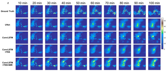
Figure 5. Radar reflectivity predictions of different strategies.

Furthermore, we applied MIR and TSS to six models to assess the universality of the proposed strategies. As shown in Table 4, we can see that TSS enhances the performance of both majority and minority classes, as Model + TSS exhibits better overall performance on CSIavg and HSSavg than the model that does not utilize TSS. Moreover, when comparing Model + TSS with Model + TSS + MIR, we observe that MIR significantly improves the performance of the minority class without compromising the majority performance and the overall image quality. By leveraging TSS and MIR, ConvLSTM (2015) outperforms the latest precipitation nowcasting models.

Table 4. Results of TSS and MIR on various models on the TAAS dataset.

Training Model	CSI↑				HSS↑				SSIM↑
	avg	20	30	40	avg	20	30	40
ConvLSTM [3]	0.148	0.330	0.100	0.014	0.225	0.476	0.173	0.026	0.689
+TSS	0.178	0.373	0.141	0.020	0.265	0.523	0.236	0.036	0.695
+TSS + MIR	0.210	0.370	0.190	0.071	0.318	0.520	0.308	0.125	0.681
UNet [20]	0.136	0.322	0.081	0.004	0.201	0.462	0.134	0.008	0.652
+TSS	0.136	0.333	0.069	0.005	0.200	0.475	0.114	0.010	0.666
+TSS + MIR	0.193	0.343	0.178	0.056	0.291	0.483	0.289	0.102	0.657
TrajGRU [11]	0.154	0.329	0.120	0.014	0.236	0.474	0.208	0.027	0.672
+TSS	0.156	0.343	0.119	0.005	0.234	0.489	0.202	0.010	0.676
+TSS + MIR	0.205	0.358	0.183	0.073	0.313	0.507	0.299	0.133	0.673
PredRNN [34] 1	0.159	0.296	0.137	0.044	0.243	0.426	0.224	0.078	0.681
+TSS	0.170	0.333	0.149	0.029	0.256	0.469	0.244	0.054	0.706
+TSS + MIR	0.199	0.356	0.186	0.056	0.301	0.502	0.300	0.100	0.704
PredRNNV2 [18]	0.174	0.355	0.155	0.013	0.262	0.503	0.258	0.025	0.695
+TSS	0.176	0.365	0.144	0.020	0.262	0.512	0.239	0.036	0.696
+TSS + MIR	0.213	0.360	0.196	0.083	0.324	0.509	0.316	0.146	0.696
DGMR [12]	0.159	0.350	0.111	0.016	0.239	0.499	0.189	0.030	0.672
+GAN 2	0.183	0.351	0.154	0.044	0.279	0.499	0.257	0.080	0.651
+TSS	0.167	0.361	0.121	0.019	0.249	0.510	0.204	0.034	0.676
+TSS + MIR	0.220	0.379	0.192	0.088	0.331	0.527	0.311	0.155	0.687

¹ PredRNN and V2 are implemented with the SS strategy. ² The DGMR is trained with GAN loss, according to the paper.

4.3. Hyperparameters of MIR and TSS

4.3.1. MIR

Table 5 presents the results of several MIR variants, including three strategies ((a), (b), and (c)) described in Section 3.2, where $\alpha$ and $\beta$ are hyperparameters controlling the reweighting factor of MIR. The results are divided into two categories, with and without TSS, demonstrating that models utilizing TSS outperform those without it. Additionally, the MIR strategy can further improve the model’s overall performance. Among the reweighting methods, our proposed $I(X^{\prime };Y)$ shows excellent performance (with the second-highest $CS{I}_{\mathrm{avg}}$) and does not require any hyperparameters. Method (a) achieves the best $CS{I}_{\mathrm{avg}}$ with $\alpha =0.05$ and $\beta =0.5$.

Table 5. MIR strategies on HKO-7. False TSS stands for the t fixed to 10.

TSS	Reweighting	CSI↑				HSS↑				SSIM↑	MSE↓
		avg	20	30	40	avg	20	30	40		$(\times {10}^{-3})$
False	None	0.246	0.439	0.261	0.036	0.350	0.589	0.397	0.064	0.739	8.069
	WMSE	0.295	0.439	0.314	0.131	0.422	0.583	0.459	0.224	0.717	12.209
	(a)$\alpha =0.1,\beta =0$	0.288	0.451	0.320	0.094	0.409	0.594	0.466	0.168	0.722	9.701
	(a)$\alpha =0.1,\beta =0.2$	0.289	0.443	0.314	0.110	0.413	0.585	0.458	0.195	0.718	11.247
	(a)$\alpha =0.2,\beta =0$	0.246	0.391	0.258	0.089	0.352	0.518	0.380	0.157	0.681	24.517
	(a)$\alpha =0.05,\beta =0$	0.278	0.460	0.314	0.059	0.392	0.607	0.464	0.106	0.726	8.086
	(a)$\alpha =0.05,\beta =0.5$	0.303	0.454	0.328	0.126	0.430	0.597	0.476	0.217	0.722	10.351
	(b)$\alpha =2$	0.260	0.450	0.291	0.040	0.368	0.596	0.436	0.071	0.724	8.995
	(c)$I(X^{\prime };Y)$	0.293	0.445	0.316	0.117	0.418	0.588	0.461	0.205	0.720	10.865
True	None	0.271	0.477	0.291	0.045	0.377	0.623	0.431	0.077	0.741	7.392
	WMSE	0.320	0.463	0.333	0.165	0.452	0.603	0.479	0.274	0.729	11.612
	(a)$\alpha =0.1,\beta =0$	0.321	0.489	0.351	0.124	0.450	0.631	0.503	0.215	0.738	7.832
	(a)$\alpha =0.1,\beta =0.2$	0.323	0.485	0.350	0.135	0.452	0.626	0.500	0.231	0.736	9.085
	(a)$\alpha =0.2,\beta =0$	0.301	0.465	0.328	0.110	0.421	0.603	0.470	0.189	0.720	9.048
	(a)$\alpha =0.05,\beta =0$	0.304	0.494	0.343	0.076	0.422	0.640	0.496	0.131	0.741	7.440
	(a)$\alpha =0.05,\beta =0.5$	0.332	0.487	0.358	0.150	0.464	0.628	0.509	0.254	0.736	9.221
	(b)$\alpha =2$	0.287	0.485	0.313	0.062	0.400	0.631	0.462	0.108	0.740	7.399
	(c)$I(X^{\prime };Y)$	0.329	0.493	0.358	0.136	0.459	0.635	0.509	0.232	0.736	9.007

4.3.2. TSS

The model’s performance is influenced by the number of training iterations L for each forecasting length t. Table 6 shows the performances of multiple TSS variants with different L. The $L=$ 1k indicates that the model was trained for 1000 iterations for each $t\in [1,10]$, with a total of 10,000 iterations. After 10,000 iterations, the model may not converge but will continue training, with t being 10 for the remaining training iterations. We proposed two other L changing strategies: $1k\to 4k$ and $4k\to 1k$. For instance, $1k\to 4k$ means $L=1000+\frac{(t-1)\times 3000}{10-1},\mathrm{hence}L\in 1000,1333,1666,\dots ,4000$. We observed that the model’s performance gradually improved after $L=4k$, so we selected $4k$ to reduce computational cost and reported the model’s performance at $4k$ in this article. The L changing strategies are illustrated in Figure 6.

Table 6. The TSS strategy with different L on ConvLSTM.

L Iterations	CSI↑				HSS↑				SSIM↑	MSE↓	Dataset
	avg	20	30	40	avg	20	30	40		$(\times {10}^{-3})$
1k	0.142	0.325	0.095	0.007	0.216	0.469	0.164	0.014	0.678	4.527	TAAS
2k	0.152	0.348	0.098	0.011	0.228	0.496	0.168	0.020	0.687	4.299
3k	0.151	0.352	0.088	0.013	0.225	0.500	0.150	0.023	0.691	4.299
4k	0.153	0.340	0.105	0.016	0.231	0.486	0.177	0.030	0.692	4.294
5k	0.173	0.367	0.134	0.018	0.258	0.515	0.226	0.032	0.693	4.297
8k	0.174	0.363	0.133	0.025	0.261	0.512	0.225	0.046	0.695	4.312
10k	0.174	0.341	0.147	0.032	0.259	0.478	0.241	0.058	0.695	4.344
1k→4k	0.152	0.357	0.088	0.012	0.226	0.506	0.150	0.022	0.686	4.374
4k→1k	0.156	0.365	0.092	0.012	0.230	0.514	0.154	0.022	0.690	4.375
1k	0.269	0.478	0.291	0.038	0.375	0.625	0.434	0.066	0.737	7.511	HKO
2k	0.265	0.469	0.283	0.043	0.373	0.617	0.425	0.076	0.738	7.449
3k	0.273	0.467	0.299	0.053	0.382	0.613	0.443	0.091	0.738	7.605
4k	0.275	0.474	0.305	0.048	0.384	0.620	0.449	0.082	0.741	7.358
5k	0.271	0.477	0.291	0.045	0.377	0.623	0.431	0.077	0.741	7.392
8k	0.273	0.480	0.287	0.053	0.382	0.626	0.428	0.092	0.742	7.323
10k	0.273	0.480	0.294	0.046	0.381	0.626	0.436	0.079	0.743	7.313
1k→4k	0.269	0.480	0.288	0.040	0.376	0.627	0.430	0.071	0.739	7.483
4k→1k	0.272	0.479	0.296	0.040	0.378	0.626	0.440	0.070	0.739	7.455
1k	0.267	0.496	0.279	0.026	0.373	0.650	0.424	0.045	0.895	2.948	ECP
2k	0.274	0.486	0.298	0.039	0.384	0.640	0.448	0.066	0.892	3.158
3k	0.282	0.510	0.292	0.044	0.391	0.662	0.437	0.075	0.898	2.789
4k	0.290	0.508	0.314	0.049	0.401	0.658	0.465	0.081	0.898	2.774
5k	0.290	0.498	0.314	0.060	0.404	0.649	0.464	0.101	0.899	2.779
8k	0.291	0.506	0.306	0.061	0.402	0.656	0.451	0.099	0.898	2.895
10k	0.308	0.523	0.337	0.064	0.424	0.673	0.493	0.106	0.899	2.781
1k→4k	0.248	0.455	0.262	0.026	0.354	0.611	0.404	0.047	0.892	3.136
4k→1k	0.279	0.511	0.286	0.039	0.384	0.662	0.426	0.065	0.898	2.819

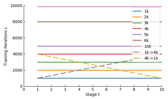
Figure 6. TSS strategies with different L. t stands for the number of frames for training in Algorithm 2.

5. Discussion

5.1. How Does MIR Work?

Figure 7 displays the visualization of $P\left(Y\right|X^{\prime })$ for TAAS. The figure exhibits the conditional distributions for five different forecasting lengths: $t=1,t=2,t=5,t=10,\mathrm{and}t=\infty$, where ∞ represents infinity. At $t=\infty$, $P\left(Y\right|X^{\prime })$ is equal to $P\left(Y\right)$, and $I(X;Y)=0$ and $H\left(Y\right|X^{\prime })=H\left(Y\right)$. We present the original $P\left(Y\right|X^{\prime })$, balanced $P\left(Y\right|X^{\prime })$, and MIR balanced $P\left(Y\right|X^{\prime })$ from top to bottom, respectively.

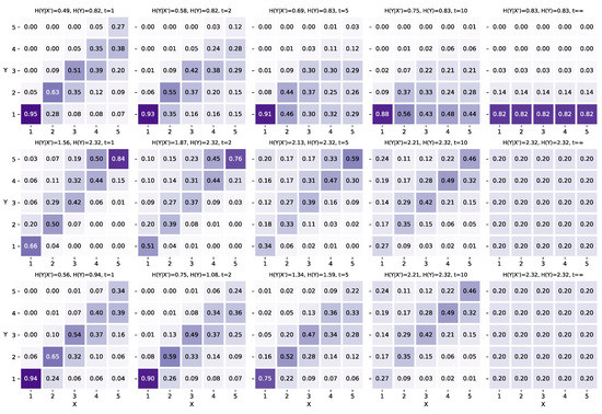
Figure 7. (Top) $P\left(Y\right|X^{\prime })$ of TAAS dataset. (Middle) $P\left(Y\right)$ balanced $P\left(Y\right|X^{\prime })$. (Bottom) MIR reweighting strategy. Smaller $H\left(Y\right|X)$ corresponds to larger $I(X;Y)$. The radar echo intensity (0–70 dBZ) is divided into five categories evenly. X and Y axes stand for the index of the category.

Five images in the top row of Figure 7 show that with t increasing, the conditional distribution $P\left(Y\right|X^{\prime })$ approaches the long-tailed distribution $P\left(Y\right)$. The mutual information is high for $t=1$ or $t=2$, which indicates that these tasks are relatively easy to learn. In contrast, for $t=5$ or $t=10$, the mutual information is low, making it difficult for the models to learn the information. When predicting an echo image occurring in the infinite future ($t=\infty$), $P\left(Y\right|X^{\prime })$ is equal to $P\left(Y\right)$.

The most simple and straightforward strategy to re-weight the training samples is to balance $P\left(Y\right)$ to a uniform distribution, and we visualize the corresponding conditional distribution $P\left(Y\right|X^{\prime })$ in the middle row of Figure 7. Compared with the original $P\left(Y\right|X^{\prime })$ in the first row, when t is either small (such as 1 and 2) or large (such as 5, 10, and ∞), all Y have a more uniformed probability. It indicates that this strategy stops the imbalanced tendency when t is large, but it changes the conditional distribution for easy-to-learn tasks at smaller t. For instance, when $t=1$, the rebalanced $P\left(Y\right|X^{\prime })$ matrix has smaller values under the diagonal than the original matrix. Since smaller t tasks are relatively easy to learn, this rebalancing strategy does not provide any benefit in this scenario.

Figure 7 presents the original conditional distribution $P\left(Y\right|X)$, the marginal distribution $P\left(Y\right)$, and the MIR-balanced $P\left(Y\right|X)$. The MIR approach leverages two main strategies: (i) preservation of the conditional distribution of high mutual information tasks, such as $t=1$ and $t=2$, and (ii) readjustment of the conditional distribution for low mutual information tasks with large t. This results in the MIR-balanced $P\left(Y\right|X^{\prime })$ having higher mutual information at smaller t and a relatively even distribution for large t.

5.2. What Is the Relationship between Mutual Information and Model Performance?

As discussed in Section 3.2, the mutual information is negatively correlated with t, and the model shows better resistance to the data imbalance problem in high mutual information scenarios. To verify the impact of the mutual information on the performance of precipitation nowcasting models, we conducted experiments on two models and three precipitation datasets with $t=$ 1, 2, 5, and 10 for the training phase. Setting $t=10$ allowed for the loss function to be calculated with all 10 predicted frames. The forecasting length of all experiments was 10 frames in the inference phase, and all the results were averaged across 10 timesteps. Table 7 records the experiment results on three datasets and the two most well-known models: an RNN model ConvLSTM and a CNN model UNet. Although ConvLSTM and UNet were proposed 7 years ago, these two models still ranked top in recent precipitation nowcasting contests due to their simple structure and good compatibility.

Table 7. Performance with different ts.

Model Strategy	Training	CSI↑				HSS↑				SSIM↑	MSE↓	Dataset
		avg	20	30	40	avg	20	30	40		$(\times {10}^{-3})$
ConvLSTM	t = 1	0.122	0.230	0.106	0.031	0.186	0.330	0.171	0.055	0.571	7.135	TAAS
	t = 2	0.142	0.306	0.116	0.004	0.216	0.442	0.198	0.007	0.591	5.626
	t = 5	0.153	0.348	0.093	0.019	0.228	0.496	0.154	0.034	0.695	4.143
	t = 10	0.148	0.330	0.100	0.014	0.225	0.476	0.173	0.026	0.689	4.485
	t = 1	0.244	0.380	0.276	0.075	0.352	0.519	0.409	0.128	0.681	11.972	HKO
	t = 2	0.240	0.422	0.264	0.035	0.341	0.567	0.397	0.060	0.724	9.542
	t = 5	0.250	0.449	0.259	0.043	0.355	0.598	0.393	0.074	0.743	7.808
	t = 10	0.246	0.439	0.261	0.036	0.350	0.589	0.397	0.064	0.739	8.069
	t = 1	0.255	0.470	0.250	0.050	0.358	0.618	0.378	0.078	0.895	3.597	ECP
	t = 2	0.269	0.480	0.277	0.049	0.371	0.623	0.408	0.083	0.888	3.800
	t = 5	0.262	0.490	0.266	0.030	0.365	0.643	0.402	0.051	0.894	3.125
	t = 10	0.243	0.461	0.262	0.006	0.345	0.618	0.406	0.011	0.893	3.224
UNet	t = 1	0.186	0.376	0.171	0.012	0.273	0.518	0.279	0.021	0.649	4.515	TAAS
	t = 2	0.190	0.382	0.188	0.001	0.275	0.524	0.301	0.001	0.656	4.407
	t = 5	0.148	0.329	0.104	0.009	0.219	0.469	0.170	0.017	0.663	4.366
	t = 10	0.136	0.322	0.081	0.004	0.201	0.462	0.134	0.008	0.652	4.591
	t = 1	0.274	0.472	0.316	0.034	0.375	0.610	0.455	0.059	0.723	7.768	HKO
	t = 2	0.271	0.470	0.314	0.029	0.372	0.611	0.457	0.049	0.723	7.296
	t = 5	0.267	0.474	0.311	0.015	0.366	0.616	0.455	0.028	0.698	7.023
	t = 10	0.248	0.449	0.279	0.017	0.346	0.591	0.416	0.031	0.684	7.071
	t = 1	0.274	0.502	0.314	0.005	0.373	0.646	0.463	0.009	0.888	3.090	ECP
	t = 2	0.284	0.521	0.326	0.005	0.385	0.668	0.477	0.010	0.880	2.879
	t = 5	0.270	0.500	0.304	0.007	0.372	0.651	0.454	0.012	0.873	2.673
	t = 10	0.244	0.454	0.269	0.009	0.343	0.605	0.409	0.016	0.874	2.778

As shown in Table 7, in terms of minority classes (CSI${}_{40}$ and HSS${}_{40}$), both ConvLSTM and UNet achieve better performance at smaller t, and worse performance at larger t. This demonstrates that larger $I(X;Y)$ tasks provide models with better data imbalance resistance.

Furthermore, according to Xu et al. (2019) [35], UNet outperforms ConvLSTM in terms of 20 dBZ, 30 dBZ, and mean squared error (MSE), indicating that UNet is more adept at capturing low-frequency information. Nevertheless, UNet exhibits inferior performance in the structural similarity index (SSIM), which may be attributed to the rough fusion and expansion of the temporal axis utilized by UNet. Additionally, the Markov chain formulation of ConLSTM enables it to produce smoother results, which could also account for its superior performance.

5.3. Mutual Information across Datasets

The mutual information among the three datasets significantly differs. In Section 3, Figure 3 indicates that mutual information of HKO-7 declines slower than TAASRAD19. Considering the goal of enhancing the amount of information available for training tasks, HKO-7 appears to be a better training set. Hence, we conducted experiments involving the exchange of training and test sets for all three datasets. As per the results presented in Table 8, the HKO-7 training variants outperformed the other variants, including the consistent results from Table 7.

Table 8. Switching the training set and the testing set of three datasets. * stands for TSS + MIR.

Model	Train	Test	${\mathbf{CSI}}_{\mathbf{avg}}\uparrow$	${\mathbf{HSS}}_{\mathbf{avg}}\uparrow$	SSIM↑	MSE↓ $(\times {10}^{-3})$
UNet	TAAS	ECP	0.263	0.362	0.867	2.915
UNet	HKO-7	ECP	0.269	0.371	0.886	2.858
ConvLSTM	TAAS	ECP	0.191	0.271	0.880	3.160
ConvLSTM	HKO-7	ECP	0.258	0.367	0.892	3.203
ConvLSTM *	TAAS	ECP	0.262	0.370	0.748	3.350
ConvLSTM *	HKO-7	ECP	0.329	0.457	0.898	2.947
UNet	TAAS	HKO-7	0.177	0.250	0.710	8.505
UNet	ECP	HKO-7	0.212	0.299	0.723	8.723
ConvLSTM	TAAS	HKO-7	0.233	0.316	0.694	8.084
ConvLSTM	ECP	HKO-7	0.240	0.326	0.719	8.405
ConvLSTM *	TAAS	HKO-7	0.242	0.337	0.649	8.210
ConvLSTM *	ECP	HKO-7	0.273	0.384	0.721	9.266
UNet	ECP	TAAS	0.144	0.212	0.458	7.390
UNet	HKO-7	TAAS	0.168	0.246	0.582	5.566
ConvLSTM	ECP	TAAS	0.138	0.209	0.379	6.932
ConvLSTM	HKO-7	TAAS	0.165	0.252	0.391	6.326
ConvLSTM *	ECP	TAAS	0.196	0.298	0.390	6.906
ConvLSTM *	HKO-7	TAAS	0.212	0.320	0.410	6.103

5.4. Limitations of Reweighting

Table 9 presents the experimental results of the WMSE variants with $t=1$, $t=10$, SS, and the TSS strategy evaluated on the TAASRAD19 dataset. The WMSE approach, which incorporates $P\left(Y\right)$ reweighting, substantially improves the CSI and HSS performance measures at 40 dBZ. However, compared to the non-weighting methods, the WMSE strategy results in an average (Average of 4 settings in Table 9) performance degradation of 5.2% for SSIM and 21.1% for MSE. For MIR, these figures are 0.04% and 3.5%, respectively, indicating that the WMSE method achieves a trade-off between image quality and minority class performance.

Table 9. Reweighting strategy on the ConvLSTM of the TAASRAD19 dataset.

Strategy	Reweighting	${\mathbf{CSI}}_{20}\uparrow$	${\mathbf{CSI}}_{40}\uparrow$	${\mathbf{HSS}}_{20}\uparrow$	${\mathbf{HSS}}_{40}\uparrow$	SSIM↑	MSE↓$(\times {10}^{-3})$
$t=1$	None	0.230	0.031	0.330	0.055	0.571	7.135
$t=10$		0.330	0.014	0.476	0.026	0.689	4.485
SS		0.327	0.018	0.469	0.033	0.648	5.050
TSS		0.373	0.020	0.523	0.036	0.695	4.253
$t=1$	WMSE	0.292	0.053	0.418	0.090	0.519	9.084
$t=10$		0.336	0.075	0.482	0.135	0.638	5.461
SS		0.334	0.090	0.479	0.159	0.629	5.700
TSS		0.370	0.088	0.518	0.155	0.671	4.946
$t=1$ *	MIR	0.230	0.031	0.330	0.055	0.571	7.135
$t=10$		0.346	0.081	0.494	0.145	0.663	4.978
SS		0.370	0.082	0.519	0.145	0.679	4.992
TSS		0.370	0.071	0.520	0.125	0.681	4.429

* MIR strategy is the same as non-weighting when t = 1.

5.5. Limitations of MIR and TSS

TSS is a curriculum learning method that trains tasks in an order of increasing difficulty. It employs the mutual information of each task to control the training sequence. However, TSS only applies to the prediction part and not the encoding part, which limits its effectiveness on separate encoder–decoder networks such as TrajGRU. ConvLSTM uses the same model parameters for each time step, whereas UNet uses different parameters for each time step. Therefore, TSS is also limited for UNet since it has specific parameters for each timestep. Additionally, UNet encodes and generates all frames simultaneously, which reduces the need for a curriculum learning style strategy, as the parameters are relatively independent. To address this, MIR weakens the reweighting factors for high mutual information tasks, reinforcing the simplest reweighting strategy. This has been successful with both RNN and CNN structured precipitation nowcasting models.

However, the approximation method in Equation (3) degrades the higher-order information of the data and adds uncertainty to the approximated $P\left(Y\right|X)$. Improving the approximation method can lead to a more precise $I(X;Y)$.

6. Conclusions and Future Work

In the precipitation nowcasting task, previous studies have attributed poor prediction performances regarding heavy rainfall samples to the data imbalance issue. We found that prediction performance is related to both mutual information (MI) and data imbalance.

In this paper, we redefined the precipitation nowcasting task at the pixel level to estimate the conditional distribution $P\left(Y\right|X)$ and the mutual information $I(X;Y)$. We found that higher $I(X;Y)$ corresponds to better data imbalance resistance. Inspired by this finding, a reweighting method, MIR, preserves more information by assigning smooth weighting factors for high $I(X;Y)$ data. MIR successfully avoids downgrading the performance of the majority class. By studying the relationship between $I(X;Y)$ and the forecasting timespan t, we found that a smaller t benefits the model’s training. Combining this feature with the merit of curriculum learning, ordered from easy to hard, we proposed a curriculum-learning-style training strategy. The experimental results demonstrated the superiority of the proposed strategies. With the help of the approximated $I(X;Y)$ and $P\left(Y\right|X)$, we also tried to explain how $P\left(Y\right)$-based reweighting works and to find an informative precipitation dataset. This work is only a preliminary exploration since $P\left(Y\right|X)$ is not fully utilized. More mutual information-based strategies remain to be discovered.

References

- Lebedev, V.; Ivashkin, V.; Rudenko, I.; Ganshin, A.; Molchanov, A.; Ovcharenko, S.; Grokhovetskiy, R.; Bushmarinov, I.; Solomentsev, D. Precipitation nowcasting with satellite imagery. In Proceedings of the 25th ACM SIGKDD International Conference on Knowledge Discovery & Data Mining, Anchorage, AK, USA, 4–8 August 2019; pp. 2680–2688. [Google Scholar]
- Sun, Z.; Sandoval, L.; Crystal-Ornelas, R.; Mousavi, S.M.; Wang, J.; Lin, C.; Cristea, N.; Tong, D.; Carande, W.H.; Ma, X.; et al. A review of Earth Artificial Intelligence. Comput. Geosci. 2022, 159, 105034. [Google Scholar] [CrossRef]
- Shi, X.; Chen, Z.; Wang, H.; Yeung, D.Y.; Wong, W.; Woo, W. Convolutional LSTM Network: A Machine Learning Approach for Precipitation Nowcasting. In Proceedings of the International Conference on Neural Information Processing Systems, Montreal, QC, Canada, 7–12 December 2015; pp. 802–810. [Google Scholar]
- Niu, D.; Huang, J.; Zang, Z.; Xu, L.; Che, H.; Tang, Y. Two-stage spatiotemporal context refinement network for precipitation nowcasting. Remote Sens. 2021, 13, 4285. [Google Scholar] [CrossRef]
- Huang, Q.; Chen, S.; Tan, J. TSRC: A Deep Learning Model for Precipitation Short-Term Forecasting over China Using Radar Echo Data. Remote Sens. 2023, 15, 142. [Google Scholar] [CrossRef]
- Tuyen, D.N.; Tuan, T.M.; Le, X.H.; Tung, N.T.; Chau, T.K.; Van Hai, P.; Gerogiannis, V.C.; Son, L.H. RainPredRNN: A New Approach for Precipitation Nowcasting with Weather Radar Echo Images Based on Deep Learning. Axioms 2022, 11, 107. [Google Scholar] [CrossRef]
- Zhang, F.; Wang, X.; Guan, J. A Novel Multi-Input Multi-Output Recurrent Neural Network Based on Multimodal Fusion and Spatiotemporal Prediction for 0–4 Hour Precipitation Nowcasting. Atmosphere 2021, 12, 1596. [Google Scholar] [CrossRef]
- Cao, Y.; Chen, L.; Zhang, D.; Ma, L.; Shan, H. Hybrid Weighting Loss for Precipitation Nowcasting from Radar Images. In Proceedings of the ICASSP 2022—2022 IEEE International Conference on Acoustics, Speech and Signal Processing (ICASSP), Singapore, 22–27 May 2022; pp. 3738–3742. [Google Scholar]
- Franch, G.; Maggio, V.; Coviello, L.; Pendesini, M.; Jurman, G.; Furlanello, C. TAASRAD19, a high-resolution weather radar reflectivity dataset for precipitation nowcasting. Sci. Data 2020, 7, 1–13. [Google Scholar] [CrossRef] [PubMed]
- Chen, L.; Cao, Y.; Ma, L.; Zhang, J. A Deep Learning-Based Methodology for Precipitation Nowcasting With Radar. Earth Space Sci. 2020, 7, e2019EA000812. [Google Scholar] [CrossRef]
- Shi, X.; Gao, Z.; Lausen, L.; Wang, H.; Yeung, D.Y.; Wong, W.; Woo, W. Deep learning for precipitation nowcasting: A benchmark and a new model. In Proceedings of the Advances in Neural Information Processing Systems, Long Beach, CA, USA, 4–9 December 2017; pp. 5617–5627. [Google Scholar]
- Ravuri, S.; Lenc, K.; Willson, M.; Kangin, D.; Lam, R.; Mirowski, P.; Fitzsimons, M.; Athanassiadou, M.; Kashem, S.; Madge, S.; et al. Skilful precipitation nowcasting using deep generative models of radar. Nature 2021, 597, 672–677. [Google Scholar] [CrossRef] [PubMed]
- Brillouin, L. Science and Information Theory; Courier Corporation: North Chelmsford, MA, USA, 2013. [Google Scholar]
- Cao, Y.; Zhang, D.; Zheng, X.; Shan, H.; Zhang, J. Mutual Information based Reweighting for Precipitation Nowcasting. In Proceedings of the ICASSP 2023—2023 IEEE International Conference on Acoustics, Speech and Signal Processing (ICASSP), Rhodes Island, Greece, 4–10 June 2023. [Google Scholar]
- Gao, Z.; Shi, X.; Wang, H.; Yeung, D.Y.; Woo, W.c.; Wong, W.K. Deep learning and the weather forecasting problem: Precipitation nowcasting. Deep Learning for the Earth Sciences: A Comprehensive Approach to Remote Sensing, Climate Science, and Geosciences; Wiley: Hoboken, NJ, USA, 2021; pp. 218–239. [Google Scholar]
- Hochreiter, S.; Schmidhuber, J. Long short-term memory. Neural Comput. 1997, 9, 1735–1780. [Google Scholar] [CrossRef]
- Sun, N.; Zhou, Z.; Li, Q.; Jing, J. Three-Dimensional Gridded Radar Echo Extrapolation for Convective Storm Nowcasting Based on 3D-ConvLSTM Model. Remote Sens. 2022, 14, 4256. [Google Scholar] [CrossRef]
- Wang, Y.; Wu, H.; Zhang, J.; Gao, Z.; Wang, J.; Philip, S.Y.; Long, M. Predrnn: A recurrent neural network for spatiotemporal predictive learning. IEEE Trans. Pattern Anal. Mach. Intell. 2022, 45, 2208–2225. [Google Scholar] [CrossRef]
- Espeholt, L.; Agrawal, S.; Sønderby, C.; Kumar, M.; Heek, J.; Bromberg, C.; Gazen, C.; Hickey, J.; Bell, A.; Kalchbrenner, N. Skillful Twelve Hour Precipitation Forecasts using Large Context Neural Networks. arXiv 2021, arXiv:2111.07470. [Google Scholar]
- Ronneberger, O.; Fischer, P.; Brox, T. U-Net: Convolutional networks for biomedical image segmentation. In Proceedings of the International Conference on Medical Image Computing and Computer-Assisted Intervention, Munich, Germany, 5–9 October 2015; pp. 234–241. [Google Scholar]
- Ayzel, G.; Scheffer, T.; Heistermann, M. RainNet v1. 0: A convolutional neural network for radar-based precipitation nowcasting. Geosci. Model Dev. 2020, 13, 2631–2644. [Google Scholar] [CrossRef]
- Agrawal, S.; Barrington, L.; Bromberg, C.; Burge, J.; Gazen, C.; Hickey, J. Machine learning for precipitation nowcasting from radar images. arXiv 2019, arXiv:1912.12132. [Google Scholar]
- Ye, Y.; Gao, F.; Cheng, W.; Liu, C.; Zhang, S. MSSTNet: A Multi-Scale Spatiotemporal Prediction Neural Network for Precipitation Nowcasting. Remote Sens. 2023, 15, 137. [Google Scholar] [CrossRef]
- Trebing, K.; Stanczyk, T.; Mehrkanoon, S. Smaat-unet: Precipitation nowcasting using a small attention-unet architecture. Pattern Recognit. Lett. 2021, 145, 178–186. [Google Scholar] [CrossRef]
- Zeng, Q.; Li, H.; Zhang, T.; He, J.; Zhang, F.; Wang, H.; Qing, Z.; Yu, Q.; Shen, B. Prediction of Radar Echo Space-Time Sequence Based on Improving TrajGRU Deep-Learning Model. Remote Sens. 2022, 14, 5042. [Google Scholar] [CrossRef]
- Xu, L.; Niu, D.; Zhang, T.; Chen, P.; Chen, X.; Li, Y. Two-Stage UA-GAN for Precipitation Nowcasting. Remote Sens. 2022, 14, 5948. [Google Scholar] [CrossRef]
- Chawla, N.V.; Japkowicz, N.; Kotcz, A. Special issue on learning from imbalanced data sets. ACM SIGKDD Explor. Newsl. 2004, 6, 1–6. [Google Scholar] [CrossRef]
- Yang, Y.; Zha, K.; Chen, Y.; Wang, H.; Katabi, D. Delving into deep imbalanced regression. In Proceedings of the International Conference on Machine Learning, Virtual, 18–24 July 2021; pp. 11842–11851. [Google Scholar]
- Johnson, J.M.; Khoshgoftaar, T.M. Survey on deep learning with class imbalance. J. Big Data 2019, 6, 1–54. [Google Scholar] [CrossRef]
- Liu, H.; Zhou, M.; Liu, Q. An embedded feature selection method for imbalanced data classification. IEEE/CAA J. Autom. Sin. 2019, 6, 703–715. [Google Scholar] [CrossRef]
- Yang, Y.; Xu, Z. Rethinking the value of labels for improving class-imbalanced learning. Adv. Neural Inf. Process. Syst. 2020, 33, 19290–19301. [Google Scholar]
- Wang, Z.; Bovik, A.C.; Sheikh, H.R.; Simoncelli, E.P. Image quality assessment: From error visibility to structural similarity. IEEE Trans. Image Process. 2004, 13, 600–612. [Google Scholar] [CrossRef] [PubMed]
- Bengio, S.; Vinyals, O.; Jaitly, N.; Shazeer, N. Scheduled sampling for sequence prediction with recurrent neural networks. In Proceedings of the Advances in Neural Information Processing Systems, Montreal, QC, Canada, 7–10 December 2015; Volume 28. [Google Scholar]
- Wang, Y.; Long, M.; Wang, J.; Gao, Z.; Yu, P.S. PredRNN: Recurrent Neural Networks for Predictive Learning using Spatiotemporal LSTMs. In Proceedings of the Advances in Neural Information Processing Systems, Long Beach, CA, USA, 4–9 December 2017; Volume 30. [Google Scholar]
- Xu, Z.Q.J.; Zhang, Y.; Xiao, Y. Training behavior of deep neural network in frequency domain. In Proceedings of the International Conference on Neural Information Processing, Bali, Indonesia, 8–12 December 2019; pp. 264–274. [Google Scholar]
Disclaimer/Publisher’s Note: The statements, opinions and data contained in all publications are solely those of the individual author(s) and contributor(s) and not of MDPI and/or the editor(s). MDPI and/or the editor(s) disclaim responsibility for any injury to people or property resulting from any ideas, methods, instructions or products referred to in the content. |
© 2023 by the authors. Licensee MDPI, Basel, Switzerland. This article is an open access article distributed under the terms and conditions of the Creative Commons Attribution (CC BY) license (https://creativecommons.org/licenses/by/4.0/).