Dielectric Fluctuation and Random Motion over Ground Model (DF-RMoG): An Unsupervised Three-Stage Method of Forest Height Estimation Considering Dielectric Property Changes

Abstract

Polarimetric Synthetic Aperture Radar Interferometry (Pol-InSAR) based forest height estimation for ecosystem monitoring and management has been developing rapidly in recent years. Spaceborne Pol-InSAR systems with long temporal baselines of several days always lead to severe temporal decorrelation, which can cause a forest height overestimation error. However, most forest height estimation studies have not considered the change in dielectric property as a factor that may cause temporal decorrelation with a long temporal baseline. Therefore, it is necessary to propose a new method that considers dielectric fluctuations and random motions of scattering elements to compensate for the temporal decorrelation effect. The lack of ground truth for forest canopy also needs a solution. Unsupervised methods could be a solution because they do not require the use of true values of tree heights as the ground truth to calculate their estimation accuracies. This paper aims to present an unsupervised forest height estimation method called Dielectric Fluctuation and Random Motion over Ground (DF-RMoG) to improve accuracy by considering the dielectric fluctuations and random motions. Its performance is investigated using Advanced Land Observing Satellite (ALOS)-1 Pol-InSAR data acquired over a German forest site with temporal intervals of 46 and 92 days. The authors analyze the relationship between forest height and different parameters with DF-RMoG and conventional models. Compared with conventional models, the proposed DF-RMoG model significantly reduces the overestimation error due to temporal decorrelation in forest height estimation according to its lowest average forest height.

1. Introduction

Forest monitoring has become increasingly important in forest studies to mitigate climate change in recent years. As one of the biophysical parameters for forest monitoring, forest height is a crucial factor in forest biomass estimation, global carbon cycle, deforestation detection, climate change investigation, and forest management [1]. The fast development of Polarimetric Synthetic Aperture Radar Interferometry (Pol-InSAR) has allowed researchers to use it in forest height estimations for more than twenty years [2,3,4]. Pol-InSAR is all-weather and all-day and combines the advantages of polarization and interferometry, making it sensitive to both height and shape of scatterers. Using Pol-InSAR technology to retrieve forest tree height has become one of the hotspots of forestry research [5].

One of the conventional and effective forest tree height estimation methods with Pol-InSAR is the three-stage process Random Volume over Ground (RVoG) model [6]. This back-scattering model simplifies each forest canopy as a volume of randomly oriented scattering particles homogeneously distributed over ground elements characterized by a constant extinction coefficient [2]. Its limitation is that it can only achieve satisfactory results using single-pass Pol-InSAR data. If RVoG is applied to single-pass data with a long temporal baseline or repeat-pass data, its result will contain severe overestimation [1,7]. The reason of this limitation is that wind-derived motion temporal decorrelation becomes a dominant component. This leads to errors in the interferometric coherence. The reason for becoming a dominant component is that RVoG assumes the forest scattering medium remains stable between different radar observations. This assumption is only applicable to short single-pass Pol-InSAR systems. In repeat-pass or single-pass with a long temporal baseline situation, temporal decorrelation severely degrades the complex interferometric coherence used for forest height estimation [8]. According to Lee et al. [9] a one-day temporal baseline can lead to a 20% to 100% overestimation of the forest height. Although efforts have been put into studying the temporal decorrelation model, it is still an intricate and long-term task because temporal decorrelation can be affected by numerous stochastic facts such as wind, biological growth, and deforestation [10].

Aiming to address this limitation, a Random Motion over Ground (RMoG) model was proposed by Lavalle et al. [11]. A Gaussian random distribution was defined with a zero mean value and vertically linear variance to describe position changes of scattering elements. Many publications show that the RMoG method successfully solves the overestimation issue in RVoG using repeat-pass Pol-InSAR data with a temporal baseline of 45 min [12,13]. However, the performance of RMoG degrades when it comes to repeat-pass spaceborne Pol-InSAR data with a longer temporal baseline. It is because dielectric temporal decorrelation becomes a dominant component in the interferometric coherence, which is neglected in both RVoG and RMoG models [1].

Although RMoG improves forest height estimation accuracy, obtaining repeat-pass data with such a short temporal baseline is hard. Temporal baselines of most spaceborne repeat-pass Pol-InSAR systems in orbit are days or even months. For instance, temporal baselines of Advanced Land Observing Satellite (ALOS)-1, ALOS-2, and RADARSAT-1/2 are at least 46 days, 14 days, and 24 days, respectively [14]. Therefore, proposing a new model for considering the dielectric fluctuation in the coherence process is necessary.

Some papers have been published with consideration of dielectric fluctuation. For instance, Lei et al. [15] proposed a coherence model that accounted for both position and dielectric property changes. Compared with the RMoG model, this model neglects the random motion of the ground scattering elements and adds two complex constants to describe the dielectric decorrelation derived from both canopy and ground. Dielectric decorrelation from canopy and ground leads to coherence magnitude reduction and the effective phase center variation. Even so, most of these papers only utilize synthetic aperture radar (SAR) magnitude information and neglect to use phase information, which may cause parameter estimation errors. It is necessary to bring up a refined forest height estimation method using both magnitude and phase information with consideration of dielectric fluctuation. Moreover, ground truth data on forest height are not always available. Therefore, this paper aims to propose an unsupervised model to improve forest height estimation accuracy. The unsupervised model does not need the ground truth of all tree heights. A model named Dielectric fluctuation and random motion over ground model (DF-RMoG) is proposed by adding the dielectric function into the RMoG model. A local compensation factor estimation procedure is added during the data processing step of the proposed model using both magnitude and phase information.

This study employs the unsupervised method and a comparison-based analysis using three models. The scope of this paper is defined to focus on canopy height and different parameters with comparisons between the three selected models. This method is chosen since there are barriers to having access to the field measurement of forest height in the chosen test site. Like many other case studies, there are no online historical recordings of most chosen sites. These limitations are discussed in Section 4 and directions for future investigations are provided. This paper is organized as follows. First, a brief introduction is given to demonstrate the development of forest height inversion methods versus different temporal baselines in Section 1. Second, the test site and data used in the experiments are introduced in Section 2.1 and Section 2.2, and the DF-RMoG model is proposed in Section 2.3. This is followed by a DF-RMoG based forest height estimation workflow with local compensation factor estimation in Section 2.4. In Section 3, forest height estimation results derived from DF-DMoG are compared with those from RVoG and RMoG from two aspects, and the local over-compensation effects are presented to indicate the necessity of the local compensation factor estimation procedure. After that, a more detailed discussion is performed to validate the superiority of the proposed DF-RMoG method and finally ends with the conclusions.

2. Methodology

2.1. Study Site

An area of a German forest of around 0.36 km² is chosen as the test site, as shown in Figure 1. The Shuttle Radar Topography Mission Digital Elevation Model (SRTM DEM) of the specific location of the test site is shown in Figure 1 [16]. The elevation of this area is around 600 to 730 m Above Mean Sea Level. The test site contains a temperate mixed mountainous forest. It is located in East Starnberg, Germany (47°58′N, 11°24′E). The dominant tree species in Germany are spruces, pines, and larches, with heights ranging from 10 to 35 m [17]. This area is chosen because it is a typical Northern forest.

2.2. Data

Microwaves can penetrate vegetation, bare soil, and sand because of their wavelengths with frequency ranges between 109 Hz (1 GHz) and 1000 GHz. A longer wavelength always has a stronger penetration ability. There are several radar bands that have been applied for different purposes because of their different wavelengths, such as X- and L-bands. As been tested effective for forest tree height estimation from several research papers [4,18], L-band data are chosen for this study. Other bands might not be as suitable as L-band for this research.

L-band (24 cm wavelength) repeat-pass spaceborne data are exploited in this research. They were collected by the Japan Aerospace Exploration Agency’s ALOS-1 (also known as PALSAR) sensor in quad-polarization mode in the years 2006 and 2007.

Table 1. Parameters of ALOS-1 data applied in this research.

Acquisition Time	Center Frequency	Polarization	Incident Angle	Temporal Baseline	Vertical Wavenumber
31 December 2006 and 15 February 2007	1270 MHz	Quad	8–30°	46 days	0.101–0.104
31 December 2006 and 2 April 2007	1270 MHz	Quad	8–30°	92 days	0.117–0.120

shows the detailed parameters of the data.

In order to validate the performance of the proposed model with different temporal baselines, ALOS-1 data acquired on three different dates (i.e., 31 December 2006, 15 February 2007, and 2 April 2007) are chosen, as shown in Table 1. These dates were selected considering the influence of seasons. Decorrelation sources are simple from December to February the following year, so this paper selected 31 December 2006 and 15 February 2007 as the test date of the data with the temporal baseline of 46 days. There are more decorrelation sources in April or in spring than in December or in winter, such as flowers. These sources will cause more estimation errors. This is the reason that 31 December 2006 and 2 April 2007 are selected for the analysis with the temporal baseline of 92 days. This design can evaluate the adoption capability of the proposed model with different decorrelation sources and situations. They are in the same mode: quad-polarimetric single-look complex (SLC). Two Pol-InSAR pairs with time intervals of 46 days and 92 days are generated according to these three dates, and this is because its repeat cycle is 46 days.

Each quad-polarimetric SLC stack contains four SAR images with different polarimetric transmit-receive modes. These modes include horizontal-transmit-and-horizontal-receive (HH), horizontal-transmit-and-vertical-receive (HV), vertical-transmit-and-horizontal-receive (VH), and vertical-transmit-and-vertical-receive (VV) modes. The permeability of cross-polarization (i.e., VH, HV) is weaker than that of co-polarization (i.e., HH, VV). In order to have a good estimation of SAR interferometric coherence, the original collected SLC SAR images are averaged by seven multi-looking operations in the azimuth direction with pixel sizes of 23 m in azimuth and 24 m in range.

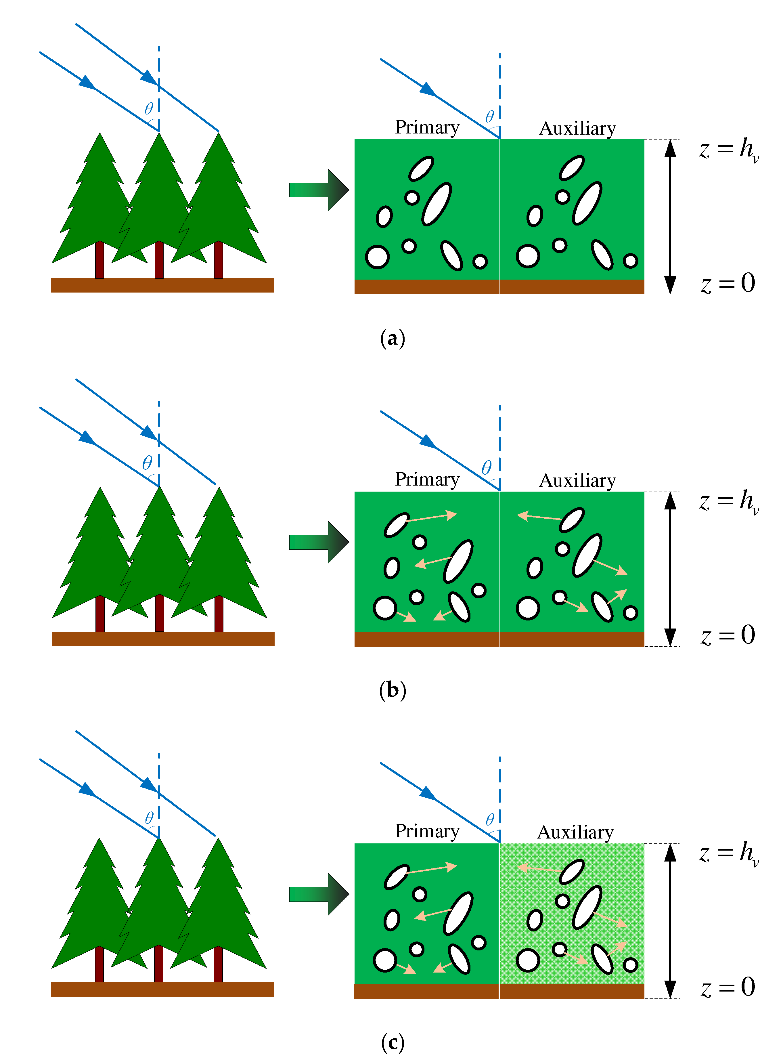
2.3. The Proposed DF-RMoG Model

The DF-RMoG model is proposed in this research to make up for the shortcomings of RVoG and RMoG models. All its equations are operated in MATLAB. It compensates for the temporal decorrelation components caused by dielectric fluctuations and random motions during a long temporal baseline in repeat-pass spaceborne Pol-InSAR systems, which are not considered in RVoG and RMoG. The detailed derivation of the DF-RMoG coherence model is demonstrated in this section.

The main difference between RVoG, RMoG, and the proposed DF-RMoG models are shown in Figure 2. Figure 2a reflects that RVoG does not consider position changes. One important improvement from RVoG to RMoG is shown in Figure 2b. RMoG defines a Gaussian motion distribution of scattering elements. The addition of the Gaussian motion feature makes it possible to compensate for the wind-induced temporal decorrelation component and, therefore, able to achieve higher forest height estimation accuracy in the condition of a temporal baseline of less than an hour. Position changes are shown as the arrows connected with the white scattering elements. Figure 2c shows that the proposed model considers random motions and dielectric fluctuations of the scattering medium caused by moisture changes, as shown in the light green background.

Equation (1) shows the scattering coherence function of the DF-RMoG model.

$${\gamma }_s=\exp \left(j{\varphi }_0\right)\frac{{\gamma }_{v\&m\&d}+{\gamma }_g^{RM}{\gamma }_g^{DF}m\left(\omega \right)}{1+m\left(\omega \right)}$$

(1)

where, ${\gamma }_s$ represents the scattering coherence function. ${\varphi }_0$ is the topographic phase. $m\left(\omega \right)$ denotes the ground-to-volume ratio depending on the polarimetric basis $\omega ,$ and j is the imaginary unit. ${\gamma }_g^{DF}$ is the ground dielectric temporal decorrelation with complex constant value. Superscript $DF$ stands for dielectric fluctuation. ${\gamma }_g^{RM}$ represents the motion temporal decorrelation of the single- and double-bounce scatterers located effectively on the ground, and the superscript $RM$ stands for random motion. It is indicated in Equation (2).

$${\gamma }_g^{RM}=\exp \left[-\frac{1}{2}{\left(\frac{4\pi }{\lambda }\right)}^2{\delta }_g^2\right]$$

(2)

where, ${\delta }_g^2$ is the variance of the ground motion distribution, $\lambda$ is the radar wavelength.

${\gamma }_{v\&m\&d}$ in Equation (1) is the motion and dielectric compensated volumetric coherence function, which is described as Equation (3).

$${\gamma }_{v\&m\&d}=\frac{{\int }_0^{h_v}{\rho }_v\left(z\right){\xi }_v\left(z\right)d_v\left(z\right)\exp \left(j{\kappa }_{z}z\right)dz}{{\int }_0^{h_v}{\rho }_v\left(z\right)dz}$$

(3)

${\rho }_v\left(z\right)$ is the volumetric attenuation function physically representing the average attenuated backscatter per vertical unit length as described in Equation (4). ${\xi }_v\left(z\right)$ denotes the volumetric motion function, which is responsible for the position changes in the volumetric scattering elements over time.

$${\rho }_v\left(z\right)=\exp \left(\frac{2\sigma z}{\cos \theta }\right)$$

(4)

where, σ is the mean extinction coefficient, $\theta$ denotes the local incidence angle.

Since the random motion of volumetric particles is assumed to be Gaussian distributed with zero mean extinction and linear variance in the vertical direction, ${\xi }_v\left(z\right)$ in Equation (3) can be described as

$${\xi }_v\left(z\right)=\exp \left[-\frac{1}{2}{\left(\frac{4\pi }{\lambda }\right)}^2\left({\delta }_g^2+\Delta {\delta }^{2}z\right)\right]={\gamma }_g^{RM}\exp \left[-\frac{1}{2}{\left(\frac{4\pi }{\lambda }\right)}^2\Delta {\delta }^{2}z\right]$$

(5)

where, $\Delta {\delta }^2$ is the vertical variance gradient of the volumetric motion distribution.

${\kappa }_z$ in Equation (3) is the vertical wavenumber. It is expressed in Equation (6).

$${\kappa }_z=\frac{4\pi }{\lambda sin\theta }\mathsf{\Delta }\theta \approx \frac{4\pi B_{\perp }}{\lambda sin\theta R}$$

(6)

where, $\theta$ denotes the local incidence angle, and $\mathsf{\Delta }\theta$ is the angle difference between two interferometric antennas. $B_{\perp }$ is the perpendicular baseline, and $R$ stands for the slant range distance.

$d_v\left(z\right)$ in Equation (3) is the volumetric dielectric function, which is responsible for the dielectric property changes in the volumetric scattering elements over time. The relationship between the moisture-deduced dielectric fluctuation and the corresponding temporal decorrelation component is complicated [19]. Dielectric decorrelation is assumed as consistent across the scattering medium, which can be described as Equation (7). Therefore, the motion and dielectric compensated volumetric coherence function of the proposed DF-RMoG model can be indicated in Equation (8).

$$d_v\left(z\right)\approx {\gamma }_g^{DF}$$

(7)

$${\gamma }_{v\&m\&d}={\gamma }_g^{DF}\cdot {\gamma }_{v\&m}={\gamma }_g^{DF}\cdot {\gamma }_g^{RM}{\gamma }_{v\&m}^{\prime }$$

(8)

where, ${\gamma }_{v\&m}$ is the motion compensated volumetric coherence function, ${\gamma }_{v\&m}^{\prime }$ is the motion compensated volumetric coherence excluding ${\gamma }_g^{RM}$.

Based on these assumptions, ${\gamma }_s$ in Equation (1) can be written as

$${\gamma }_s=\exp \left(j{\varphi }_0\right)\frac{{\gamma }_{v\&m\&d}+{\gamma }_g^{RM}{\gamma }_g^{DF}m\left(\omega \right)}{1+m\left(\omega \right)}=\exp \left(j{\varphi }_0\right){\gamma }_g^{RM}{\gamma }_g^{DF}\left({\gamma }_{v\&m}^{\prime }+\frac{m\left(\omega \right)}{m\left(\omega \right)+1}\left(1-{\gamma }_{v\&m}^{\prime }\right)\right)$$

(9)

To make Equation (9) more applicable to the forest height estimation, this research regards the dielectric decorrelation phase $\Delta \varphi =\arg \left({\gamma }_g^{DF}\right)$ as an error to the topographic phase ${\varphi }_0$, and meanwhile integrates the magnitudes of the ground dielectric and motion temporal decorrelation together as the decorrelation compensation factor, which is also the radius of the internal coherence circle $r_{\mathrm{int}}=\left|{\gamma }_g^{RM}{\gamma }_g^{DF}\right|$.

$$\begin{array}{c}{\gamma }_s=\exp \left(j{\varphi }_0\right){\gamma }_g^{RM}{\gamma }_g^{DF}\left({\gamma }_{v\&m}^{\prime }+\frac{m\left(\omega \right)}{m\left(\omega \right)+1}\left(1-{\gamma }_{v\&m}^{\prime }\right)\right)\\ =\exp \left[j\left({\varphi }_0+\Delta \varphi \right)\right]\left|{\gamma }_g^{RM}{\gamma }_g^{DF}\right|\left({\gamma }_{v\&m}^{\prime }+\frac{m\left(\omega \right)}{m\left(\omega \right)+1}\left(1-{\gamma }_{v\&m}^{\prime }\right)\right)\\ =\exp \left(j{\varphi }_0^{\prime }\right)r_{\mathrm{int}}\left({\gamma }_{v\&m}^{\prime }+\frac{m\left(\omega \right)}{m\left(\omega \right)+1}\left(1-{\gamma }_{v\&m}^{\prime }\right)\right)\end{array}$$

(10)

where, ${\varphi }_0^{\prime }$ is the intersection phase. ${\gamma }_{v\&m}^{\prime }$ in Equation (10) can be further deduced as

$$\begin{array}{c}{\gamma }_{v\&m}^{\prime }=\frac{{{\displaystyle \int }}_0^{h_v}\exp \left(\frac{2\sigma z}{\cos \theta }\right)\exp \left[-\frac{1}{2}{\left(\frac{4\pi }{\lambda }\right)}^2\Delta {\delta }^{2}z\right]\exp \left(j{\kappa }_{z}z\right)dz}{{{\displaystyle \int }}_0^{h_v}\exp \left(\frac{2\sigma z}{\cos \theta }\right)dz}\\ =\frac{2\sigma \left(\exp \left[2\sigma -\frac{1}{2}{\left(\frac{4\pi }{\lambda }\right)}^2\Delta {\delta }^2\cos \theta +j{\kappa }_z\cos \theta \right]\frac{h_v}{\cos \theta }-1\right)}{\left(2\sigma -\frac{1}{2}{\left(\frac{4\pi }{\lambda }\right)}^2\Delta {\delta }^2\cos \theta +j{\kappa }_z\cos \theta \right)\left(\exp \left(\frac{2\sigma h_v}{\cos \theta }\right)-1\right)}\end{array}$$

(11)

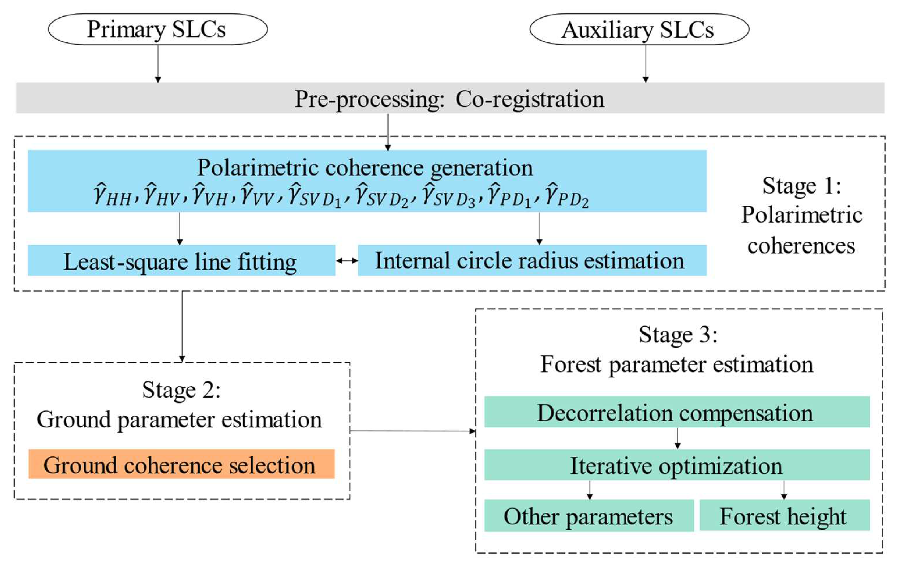
2.4. Refined Forest Height Estimation Workflow

A refined forest height estimation workflow according to the proposed DF-RMoG model is stated in this section. It can be concluded from Equations (10) and (11) that the scattering coherence of DF-RMoG is determined by six real parameters (i.e., ${\varphi }_0^{\prime },r_{\mathrm{int}},m\left(\omega \right),\sigma ,\Delta {\delta }^2,h_v$). The underdetermined problem in the forest height estimation based on the DF-RMoG model needs to be solved by at least five polarimetric coherences. This is because each polarimetric coherence provides both magnitude and phase observations with two degrees of freedom (DOF) and contains one unknown parameter (i.e., new ground-to-volume ratio).

Solving an equation question with ten unknown parameters is time-consuming, and some local optimal solutions derived from iterative optimization may cause numerous estimation errors. Therefore, based on the basic concept of the three-stage process from RVoG, this research combines geometrical features of the DF-RMoG coherence result line with the mathematical equations in Equation (12) and proposed a refined forest height estimation workflow.

$$f\left({\varphi }_0^{\prime },r_{\mathrm{int}},\sigma ,\Delta {\delta }^2,h_v,m_1,m_2,m_3,m_4,m_5\right)\mapsto \left({\gamma }_1,{\gamma }_2,{\gamma }_3,{\gamma }_4,{\gamma }_5\right)$$

(12)

where, $h_v$ is the forest height, $m_i,i=1,2,\dots ,5$ are the ground-to-volume ratios associated with the coherences ${\mathit{\gamma }}_i,i=1,2,\dots ,5$.

The proposed workflow contains three main stages as summarized in Figure 3. The grey rectangle is the pre-processing before polarimetric coherence generation. The blue parts of Stage 1 are core procedures related to the polarimetric coherences, the orange part of Stage 2 is used for ground parameter estimation, and the green parts of Stage 3 are about the forest parameter estimation.

The first stage is to find the best-fit coherence line through the least-square fitting with internal circle radius estimation. Multiple polarimetric coherences are utilized to achieve better least-square fitting performance with four polarizations, three singular value decomposition (SVD), and two Pauli decomposition (PD) polarizations [20,21,22]. Instead of the unit circle used in conventional methods, this workflow locates the ground coherence point through the intersections between the coherence line and the internal circle. This is because the ground dielectric and motion temporal decorrelation in the DF-RMoG coherence makes the ground coherence point curve towards the origin. As to realize this, the estimation of the radius of the internal circle $r_{\mathrm{int}}$ (ground decorrelation compensation factor) is necessary. Considering that the internal circle should cover all coherence observations, a local estimation method is proposed by approximating the internal circle radius as the largest polarimetric coherence magnitude in each pixel, as shown in Equation (13).

$$r_{\mathrm{int}}=\max \left\{\left|{\widehat{\gamma }}_{HH}\right|,\left|{\widehat{\gamma }}_{HV}\right|,\left|{\widehat{\gamma }}_{VH}\right|,\left|{\widehat{\gamma }}_{VV}\right|,\left|{\widehat{\gamma }}_{SV{D}_1}\right|,\left|{\widehat{\gamma }}_{SV{D}_2}\right|,\left|{\widehat{\gamma }}_{SV{D}_3}\right|,\left|{\widehat{\gamma }}_{P{D}_1}\right|,\left|{\widehat{\gamma }}_{P{D}_2}\right|\right\}$$

(13)

where, ${\widehat{\gamma }}_{HH},{\widehat{\gamma }}_{HV},{\widehat{\gamma }}_{VH},{\widehat{\gamma }}_{VV}$ are the polarimetric coherence observations, ${\widehat{\gamma }}_{SV{D}_1},{\widehat{\gamma }}_{SV{D}_2},{\widehat{\gamma }}_{SV{D}_3}$ are the SVD observations, and ${\widehat{\gamma }}_{P{D}_1},{\widehat{\gamma }}_{P{D}_2}$ are the PD observations.

In the second stage, the correct ground coherence point needs to be selected for further processing. Theoretically, there are two intersection points between the coherence line and the internal circle. One is the ground coherence point, and the other is the so-called false solution. Practically, the further a polarimetric coherence locates toward the ground coherence, the lower its ground-to-volume ratio. Therefore, the right solution can be selected by the intersection with a long distance from the polarimetric coherence point with the least ground backscatter in the visible scale. Therefore, two parameters (${\varphi }_0^{\prime },r_{\mathrm{int}}$) are determined in the above inverse problem where the phase component can be further used for the tomographic reconstruction. This is outside the scope of this paper. However, it is worth noting that during the estimation of the ground coherence, the corresponding ground-to-volume ratio is approximated as infinite, which means in this condition, the polarimetric channel introduces two DOFs without any extra unknown parameter. Therefore, after the determination of the ground coherence point, the ten-dimensional inverse problem in Equation (12) can be simplified as

$$f\left(\sigma ,\Delta {\delta }^2,h_v,m_1,m_2,m_3\right)\mapsto \left({\gamma }_1,{\gamma }_2,{\gamma }_3\right)$$

(14)

The last stage of the workflow is to solve the nonlinear equations with three unknown parameters, which is the forest parameter estimation. Considering that the magnitudes of the SVD and PD coherences are more likely to be selected as the internal circle radius and the reciprocal theory assumes ${\widehat{\gamma }}_{HV}\approx {\widehat{\gamma }}_{VH}$ [23,24,25], thus, the inverse problem can be solved by the following equation.

$$\left\{\begin{array}{c}{\widehat{\gamma }}_{HH}\cdot \frac{\exp \left(-j{\widehat{\varphi }}_0^{\prime }\right)}{{\widehat{r}}_{\mathrm{int}}}=\frac{{\gamma }_{v\&m}^{\prime }\left(\sigma ,\Delta {\delta }^2,h_v\right)+m_1}{1+m_1}\\ \frac{{\widehat{\gamma }}_{HV}+{\widehat{\gamma }}_{VH}}{2}\cdot \frac{\exp \left(-j{\widehat{\varphi }}_0^{\prime }\right)}{{\widehat{r}}_{\mathrm{int}}}=\frac{{\gamma }_{v\&m}^{\prime }\left(\sigma ,\Delta {\delta }^2,h_v\right)+m_2}{1+m_2}\\ {\widehat{\gamma }}_{VV}\cdot \frac{\exp \left(-j{\widehat{\varphi }}_0^{\prime }\right)}{{\widehat{r}}_{\mathrm{int}}}=\frac{{\gamma }_{v\&m}^{\prime }\left(\sigma ,\Delta {\delta }^2,h_v\right)+m_3}{1+m_3}\end{array}\right.$$

(15)

As to estimate the unknowns in Equation (15), the iterative optimization procedure is carried out by minimizing the least square distance between the DF-RMoG predicted and the observed coherences [1].

As mentioned in several papers [9,26,27,28,29], for repeat-pass Pol-InSAR data with temporal baselines in the order of days or months, the major problem of the traditional methods is their proneness to overestimate the forest height. Thus, two parameters, namely, the average (AVE) height and the relative decrease percentage (RDP) are selected as the main assessment criteria.

$$AVE=\frac{{\sum }_{k=1}^n{h}_v\left(k\right)}{k},RDP=\frac{{\sum }_{k=1}^n\left(h_{v_1}\left(k\right)-h_{v_2}\left(k\right)\right)}{{\sum }_{k=1}^n{h}_{v_1}\left(k\right)}\times 100\%$$

(16)

where, $h_v\left(k\right)$ is the retrieved forest height at the $k$th pixel of the sample map.

The values of the parameters in this research to fit ALOS-1 PALSAR sensors are ${\kappa }_z=0.1{\mathrm{m}}^{-1}$, $m\left(\omega \right)=0$, $\sigma =0.2{\mathrm{dB}\mathrm{m}}^{-1}$, ${\delta }_g^2=3.6\times {10}^{-5}$, $\lambda =0.23\mathrm{m}$, ${\gamma }_g^{DF}=0.9e^{-0.1i}$, $\theta ={45}^{\circ }$.

3. Results

3.1. Analyses of Coherence Results between Three Models

Quantitative analyses of different coherence models are carried out from both numerical and geometrical aspects in this research, including RVoG, RMoG, and the proposed DF-RMoG.

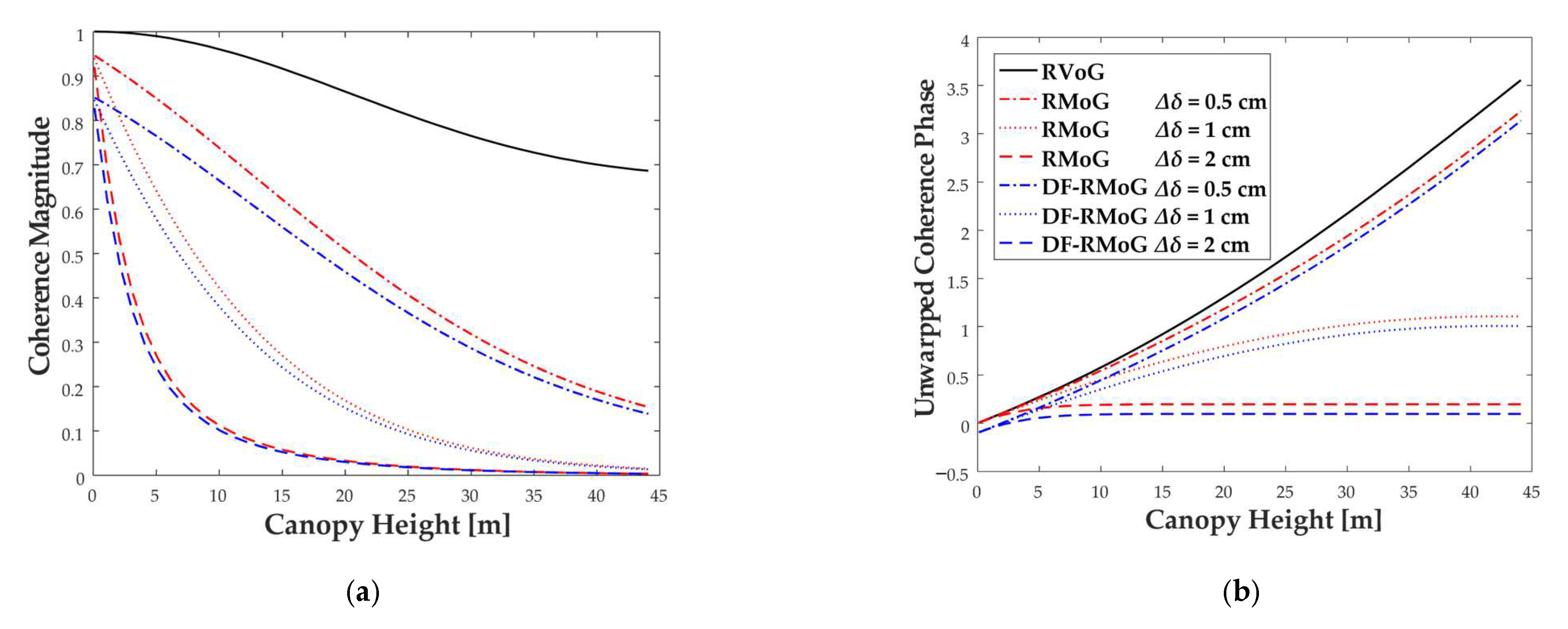
3.1.1. Numerical Analysis

The numerical aspect analyzes the relationship between canopy height and different parameters with RVoG, RMoG, and DF-RMoG models. Results are based on the scattering coherence functions in Section 2.3. The results of magnitude and unwrapped phase of RVoG coherence are shown as a reference to RMoG and DF-RMoG. Different variance gradients of the Gaussian motion distribution, including 0.005 m, 0.01 m, and 0.02 m, are applied in RMoG and DF-RMoG models, as shown in Figure 4, with different types of lines. Moreover, canopy height is set to vary continuously from 0 to 45 m. The detailed results are shown in Figure 4.

As shown in Figure 4a, the magnitudes of RVoG, RMoG, and DF-RMoG coherences start from different initial values (DF-RMoG < RMoG < RVoG = 1), and gradually decrease with the increase in canopy height. The ground motion decorrelation component causes the smaller initial value of the RMoG magnitude. Similarly, for the DF-RMoG model, besides the motion factor, the dielectric fluctuation aggravates the temporal decorrelation and thus causes an even smaller initial magnitude. Moreover, in comparison with the RVoG coherence, the RMoG, and the DF-RMoG magnitudes decrease more rapidly to zero when increasing the value of the motion variance gradient.

Similar to Figure 4a,b shows that the coherence results of unwrapped phases of RVoG, RMoG, and DF-RMoG also started from different initial values (DF-RMoG ≠ RMoG = RVoG = 0). The different results of DF-RMoG model might be caused by the phase error from the ground dielectric temporal decorrelation. Compared with the RVoG coherence result, Figure 4b validates that increasing the motion variance gradient value can slow the rising speed of RMoG and the DF-RMoG phases.

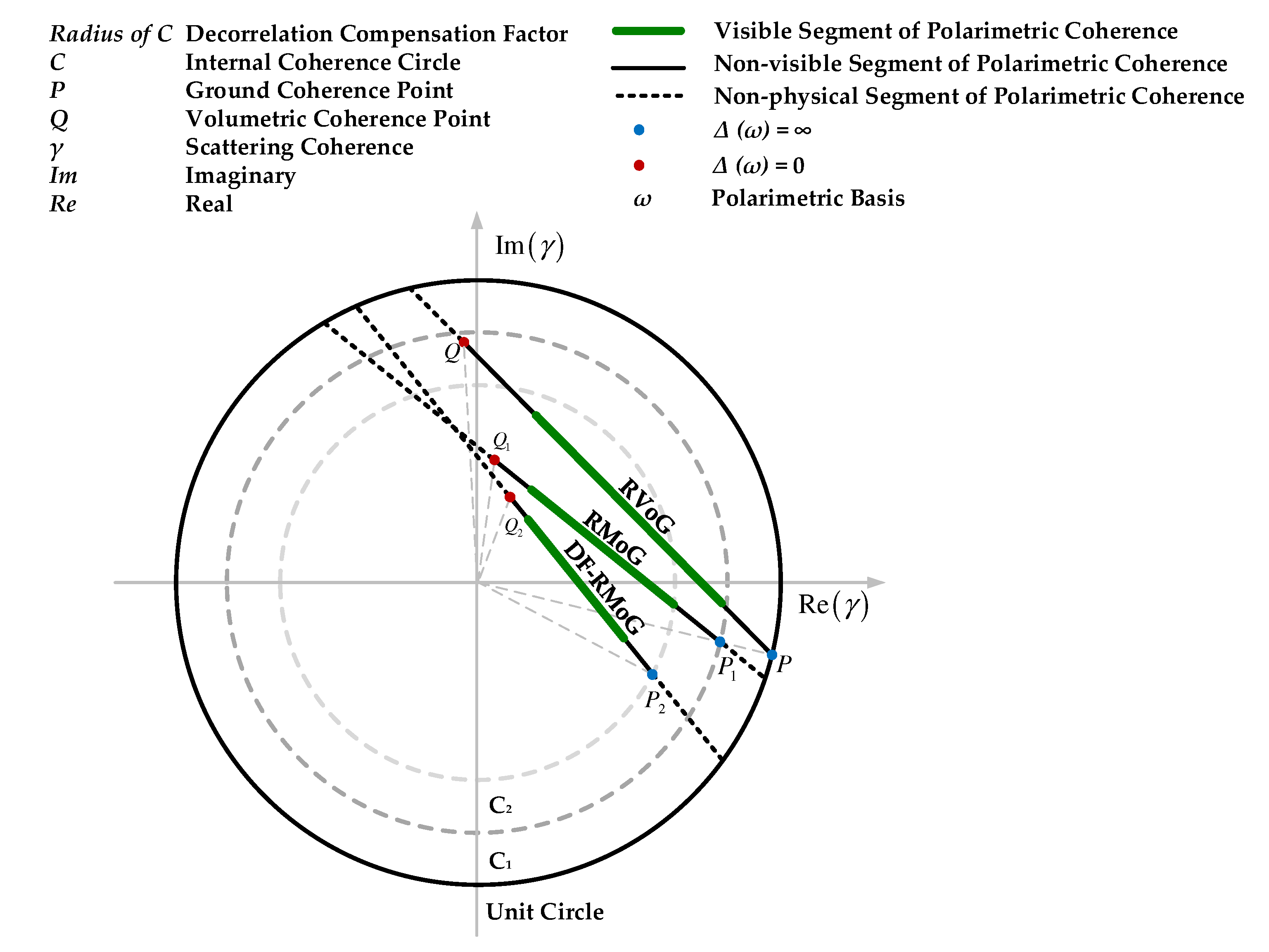
3.1.2. Geometrical Analysis

Geometrically, the coherence loci of RVoG, RMoG, and DF-RMoG models are plotted versus different polarizations, as demonstrated in Figure 5. The process for creating Figure 5 has been explained in the second stage of Section 2.4.

Figure 5 shows that the scattering coherence in the RVoG model linearly varies with the ground-to-volume ratio (polarization), which can be approximated as a line in the complex coherence plane. Theoretically, the value of the ground-to-volume ratio ranges from zero to infinity. The result reflects that if it becomes zero, all scattering components are from the volume layer, and in this condition, the coherence can be described as point Q ($\exp \left(j{\varphi }_0\right){\gamma }_v$). If it becomes infinite, all scattering contributions are from the ground, and corresponding scattering coherence comes to point P ($\exp \left(j{\varphi }_0\right)$). The angle of point P represents the topographic phase ${\varphi }_0$ and can be extracted through the intersection between the locus line and the unit circle. PQ is the physical segment of the RVoG coherence line, where the green part is the visible part that can be observed practically.

In comparison with the RVoG model, although the random motion property of the RMoG model changes the locations of the polarimetric coherences in the complex plane, the integral locus remains linear and varies with the ground-to-volume ratio, as demonstrated in Figure 5. Similarly, when the ground-to-volume ratios are zero and infinite, the coherences become point Q₁ ($\exp \left(j{\varphi }_0\right){\gamma }_{v\&m}$) and point P₁ ($\exp \left(j{\varphi }_0\right){\gamma }_g^{RM}$), respectively. P₁Q₁ is the physical segment of the RMoG locus with the visible part marked as green. Instead of the unit circle, P₁ is the intersection point between the coherence line and the internal circle C₁ whose phase is identical to point P because the ground motion decorrelation is a real number less than 1. In addition, the radius of point Q₁ is much shorter than that of point Q due to the motion decorrelation from the volume layer.

The locations of the polarization coherences of the DF-RMoG model are also influenced by the dielectric decorrelation besides the motion decorrelation. Figure 5 also shows that the introduction of the dielectric factor did not break the linear feature of DF-RMoG coherence locus. The physical segment of the DF-RMoG locus is demonstrated in Figure 5 with endpoints Q₂ ($\exp \left(j{\varphi }_0\right){\gamma }_{v\&m\&d}$) and P₂ ($\exp \left(j{\varphi }_0\right){\gamma }_g^{RM}{\gamma }_g^{DF}$) corresponding to the zero and infinite ground-to-volume ratio, respectively. In Figure 5, the DF-RMoG coherence line intersects with the internal circle C₂ at point P₂. The phase of P₂ is the sum of the topographic phase and the phase error $\mathsf{\Delta }\varphi$ from the ground dielectric decorrelation. The radius $r_{\mathrm{int}}$ of P₂ is smaller than that of P₁ because the magnitude of ${\gamma }_g^{DF}$ for P₂ is less than one. Similarly, the radius of Q₂ is also smaller than that of Q₁ due to the dielectric decorrelation from the volume layer for Q₂. Hence, Figure 5 shows that the proposed method performed best.

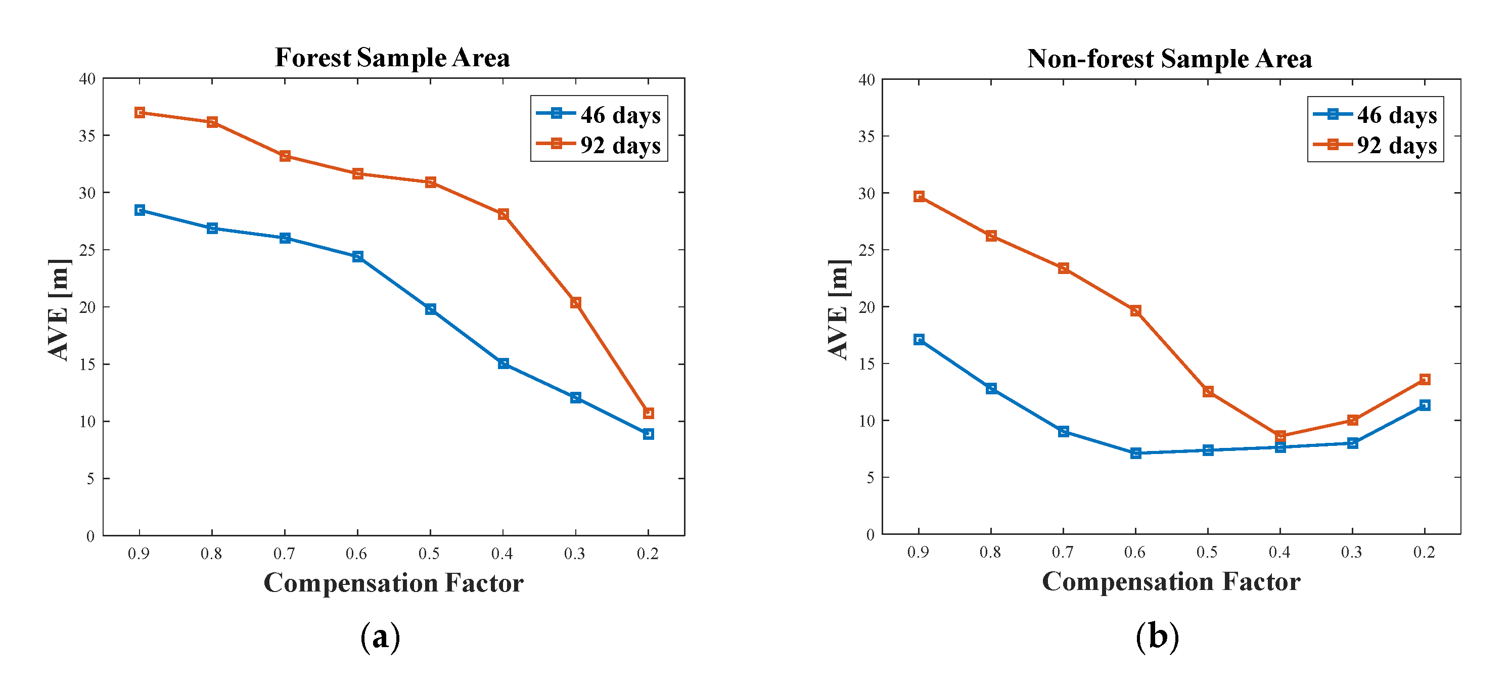
3.2. Results of DF-RMoG with Different Compensation Factor Values for Dielectric Fluctuations

This section presents and analyzes forest height estimation results from the proposed DF-RMoG model with globally consistent compensation factors (internal circle radiuses). These results are stated to analyze the effect of the compensation for dielectric fluctuations of the scattering medium caused by moisture changes and the necessity of the local compensation factor estimation.

3.2.1. Results of Data with the Temporal Baseline of 46 Days

The forest height estimation of Pol-InSAR data with a temporal baseline of 46 days are shown in Figure 6. They are the results with different sampled compensation factor values, including 0.9, 0.7, 0.5, and 0.3, as shown in Figure 6a–d, respectively.

In Figure 6, x and y axes represent the column and row of the inversed forest height maps, respectively. The color bar is the scale of the tree’s height. It is obvious in Figure 6a,b that the descending compensation factor integrally suppresses the overestimation errors in both forest and non-forest areas. However, as it continues to drop, the over-compensation problem first appears in the forest area, which is presented as the local height underestimation, as shown in Figure 6c. After that, in Figure 6d, the over-compensation occurs in the non-forest area, which is presented as the height overestimation, and in the meantime, the forest area is completely over-compensated.

3.2.2. Results of Data with Temporal Baseline of 92 Days

The forest height maps derived from Pol-InSAR data with a temporal baseline of 92 days are presented in Figure 7, where the compensation factor values are the same as those in Figure 6. Figure 7a–d shows the results with these four values. Similar to the results shown in Figure 6, the descending compensation factor from 0.9 to 0.5 integrally suppresses the overestimation error of the whole image, as shown in Figure 7a–c. Then, the local over-compensation occurs in both forest and non-forest areas when the factor continues to drop to 0.3, as shown in Figure 7d.

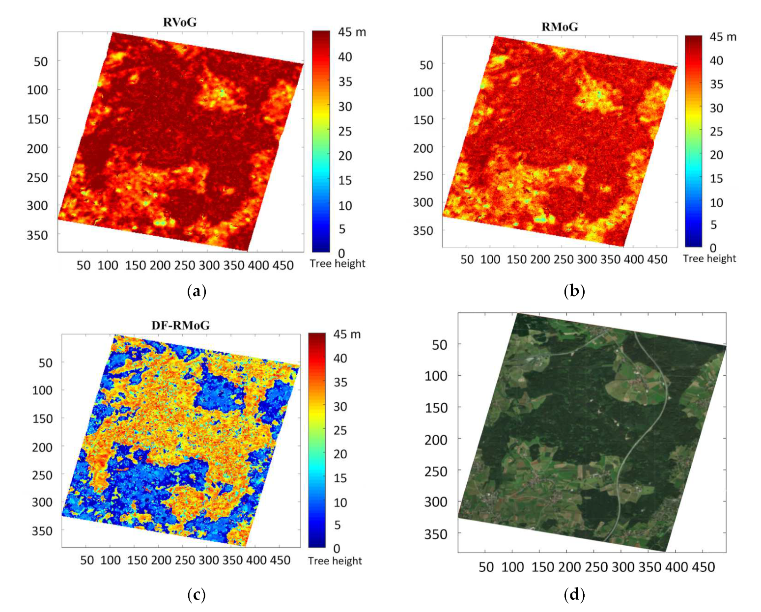
3.3. Comparison of Performance of Forest Height Estimation Results between Three Models

In order to evaluate the performance of the proposed DF-RMoG model that considers the local compensation factor for forest height estimation, it is compared with two models with the scatter plots between their results. The other two models are RVoG and RMoG. Two different temporal baselines are chosen for comparison in this research, including 46 and 92 days. The value of the factor in DF-RMoG was chosen according to the experience of the experiments stated in Section 3.2.

3.3.1. Experiments with the Temporal Baseline of 46 Days

Figure 8 displays the forest height maps obtained from the three models using Pol-InSAR data with a temporal baseline of 46 days. Figure 8a depicts the result of RVoG, where a large portion is marked in red. Figure 8b indicates the result of RMoG, which has a smaller red area compared to RVoG. Figure 8c shows the result of DF-RMoG, which reveals the least number of red pixels among the three figures. Figure 8d is the optical image of the study site from Google Earth. To present a more intuitive comparison between the three models, the scatter plots of the tree height results of RVoG versus RMoG, RVoG versus DF-RMoG, and RMoG versus DF-RMoG are shown in Figure 9a–c, respectively. The red line is x = y line, which is the identity line. The coordinate values of each blue point are the two height result values of the two chosen models. The height values shown in Figure 8 were applied as the values in Figure 9.

It can be concluded from Figure 9a that the RVoG method tends to overestimate the forest height compared with the RMoG method because all the scatter plots are located above the identity line. Furthermore, the differences between the height values from RVoG and RMoG are stable between 1.34 m and 7.68 m within the forest height interval.

Similarly, as shown in Figure 9b, the proposed DF-RMoG method is more effective in reducing the overestimation error than the RVoG method because the scatter plots are located much further to the identity line. However, in Figure 9b, the differences between the RVoG and DF-RMoG heights decrease with the ascending forest height. This is because the decorrelation compensation procedure in the DF-RMoG method is more applicable in ground areas instead of forest areas.

The same conclusion can be summarized in Figure 9c that the proposed DF-RMoG method can largely decrease the overestimation errors compared with RMoG. This is because the scatter plot locates overall above the identity line in Figure 9c. This agrees well with the results in Figure 9a,b. Meanwhile, for the same reason, the differences between the RMoG and DF-RMoG heights decrease with the ascending forest height.

3.3.2. Experiments with the Temporal Baseline of 92 Days

The forest height maps derived from the Pol-InSAR data with a temporal baseline of 92 days are demonstrated in Figure 10a–c. Figure 10d is the optical image of the study site from Google Earth, which is the same as Figure 8d. The color comparison between Figure 8 and Figure 10 reflects that the retrieved forest heights with 92 days are overall higher than those with 46 days. It is reasonable because the additional temporal baseline aggravates the overestimation error.

Similar to Section 3.3.1, the corresponding scatter plots of RVoG heights versus RMoG heights, RVoG heights versus DF-RMoG heights, and RMoG heights versus DF-RMoG heights, are generated as Figure 11a–c.

Moreover, it can be concluded from Figure 11a that the differences between the RVoG height and the RMoG height remain stable between 0.63 m and 6.94 m within the forest height interval, which is consistent with the results in Figure 11a. In addition, the same conclusion can be drawn as 46 days that in comparison with the traditional RVoG and RMoG methods, the DF-RMoG method is more capable of suppressing the overestimation errors in the ground areas instead of the forest because the differences in Figure 11b,c decrease with the ascending forest height.

The difference between Figure 9 and Figure 11 is that for the scatter plots involving the DF-RMoG heights, the locations of 92 days are much further to the identity line in comparison with 46 days, which indicates that the DF-RMoG method performs better in the condition of longer temporal baseline.

4. Discussion

4.1. Local Over-Compensation

Results of Section 3.1 show that the result values and the DF-RMoG model’s convergence are better than those of the other two. Hence, it can be concluded that DF-RMoG model performs best among these three models. Moreover, results from Section 3.2 can be concluded that the local over-compensation effect varies with different scattering elements (i.e., forest and non-forest) and different temporal baselines, and thus it is necessary to bring up a local estimation method for the compensation factor. However, the complicated relationship between the temporal and the compensation factors makes it hard to establish the mathematical estimation model directly.

As to summarize how the local over-compensation occurs with the descending compensation factor, the DF-RMoG method with a globally consistent compensation factor uniformly sampled from 0.2 to 0.9 is performed on the Pol-InSAR data with temporal baselines of 46 days and 92 days. Related AVE values of these forest height estimation results are calculated and plotted versus the compensation factor in both forest and non-forest sample areas to present the different over-compensation effects of different scattering elements.

As presented in Figure 12, the blue lines represent the variation of the AVE values derived from the forest height maps in Figure 6 with a temporal baseline of 46 days. In forest samples, a rapid drop occurs in the AVE value when the compensation factor approaches 0.6, and in non-forest areas, the AVE value first decreases and then increases with the descending compensation factor.

On the other hand, related AVE values derived from the forest height maps in Figure 7 with a temporal baseline of 92 days are also calculated and plotted as the red lines in Figure 12. Obviously, the variation trend of 92 days is the same as 46 days, but the rapid drop point in the forest area becomes 0.4, and the minimum point in the non-forest area comes later than the blue line. The main reason for this is that the temporal decorrelation of 92 days is much more severe than 46 days, and therefore the initial over-compensation factor is smaller. It is also the main reason for the overall higher AVE values of 92 days in both sample areas.

Furthermore, the different AVE variations in the forest and non-forest areas for both 46 and 92 days indicate that the optimal compensation factor varies with different ground scattering features, which validates the necessity of the local compensation factor estimation procedure from another aspect.

4.2. Forest Height Estimation

The AVEs and RDPs of the results in Figure 8 and Figure 10 are calculated to make a quantitative comparison among different forest height estimation methods. Figure 13a,b are the AVEs of the inversed height in the forest and non-forest areas, where the blue bars are the results of 46 days, and the yellow bars are 92 days. The AVE values are labeled above the histogram bars, which are proportional to the bar height.

For the temporal baseline of 46 days, in both forest and non-forest samples, the AVEs follow a decreasing trend with different forest height estimation methods. In the forest areas, the RDPs of RVoG and RMoG heights versus DF-RMoG heights are 33.4% and 19.8%. Similarly, in the non-forest areas, corresponding RDPs are 69.4% and 63.4%. These results indicate that, on the one hand, the DF-RMoG method is more effective in suppressing the over-estimation errors compared with the RVoG and the RMoG methods in both forest and non-forest areas. On the other hand, it can be concluded from the different RDPs in different sample areas that the performance of the DF-RMoG method is better in non-forest areas compared with forest areas which are consistent with the results in the scatter plots mentioned above.

For the temporal baseline of 92 days, in both forest and non-forest samples, the AVEs still follow a decreasing trend at 46 days. Likewise, the RDPs of the RVoG and RMoG heights versus DF-RMoG heights are calculated as 32.8% and 26.8% in the forest samples and 75.9% and 72.9% in the non-forest samples. These results agree with the above-mentioned conclusion that the DF-RMoG method suppresses the overestimation errors more effectively than the RVoG and the RMoG methods, especially in non-forest areas.

Furthermore, comparisons can also be carried out between the results of 46 days and 92 days. In forest and non-forest areas, the AVEs of 92 days are overall higher than that of 46 days because the additional temporal baseline aggravates the overestimation problem. In the forest areas, the RDPs of 92 days versus 46 days for the RVoG, RMoG, and DF-RMoG heights are 11.3%, 19.7%, and 12.0%, respectively. Similarly, in the non-forest areas, the RDPs of 92 days versus 46 days are 29.0%, 33.5%, and 10.0%. For the RVoG and RMoG heights, there are significant differences between the RDPs in the forest and non-forest areas. However, RDPs of the DF-RMoG height are stable at around 10% in both forest and non-forest areas. These results indicate that the DF-RMoG method is more adaptive to different ground scattering features and temporal baselines than the RVoG and RMoG methods.

What is worth noting is that, besides the dielectric fluctuation and random motion for higher forest height estimation accuracy, other temporal factors also need to be considered to compensate for the decorrelation effect. However, compared with the traditional coherence model, the proposed model is more delicate so that it can be further used for bushfire and deforestation detection along with other remote sensing techniques.

L-band is more suitable for forests because of its strong penetrability, so it was chosen in this paper. A limitation of accessing data is that most available L-band data in research are only ALOS and SAOCOM-L. This paper only has access to ALOS, so only ALOS data were applied. There are some L-band SAR satellites that have been launched recently or will be launched soon, such as NISAR-L, biomass, L-SAR, Rose-L, and Tandem-L. The DF-RMoG model can also be used on these satellites if these data are available in future. Another limitation of this paper is the absence of ground truth data. The ALOS-1 data used in this paper were collected in 2006 and 2007. However, Global Ecosystem Dynamics Investigation (GEDI) mission was launched in 2018, which is a decade later than the ALOS-1 data acquisition. Therefore, GEDI data were not applied as the ground truth in this paper. Future studies could apply ICESAT or GEDI data as ground truth data for large-scale forest height estimation.

5. Conclusions

The RMoG model has been widely applied to forest height estimation using single-pass Pol-InSAR data with short temporal baselines. However, when it comes to repeat-pass spaceborne Pol-InSAR systems with longer temporal baselines of days or months, severe temporal decorrelation can largely restrain the performance of RMoG. In order to address this problem, the unsupervised DF-RMoG model is proposed in this paper by introducing a dielectric function into the RMoG coherence. This model takes account of both dielectric fluctuation and the random motion of the scattering medium. The DF-RMoG forest height estimation method considers local compensation factor estimation, which is often ignored by most studies. Its performance is investigated using ALOS-1 PALSAR data acquired over a German forest site with temporal baselines of 46 and 92 days. The characteristics of different coherence models are analyzed from both numerical and geometrical aspects, and the local over-compensation effects are presented to indicate the necessity of the local compensation factor estimation procedure. Conclusions can be drawn from the estimation results that the local compensation factor estimation step effectively avoids the over-compensation problem compared with the globally consistent compensation. Additionally, compared with RVoG and RMoG models, the DF-RMoG model can effectively reduce overestimation errors caused by temporal decorrelation in forest height estimation. The reductions in the DF-RMoG model with a 46-day temporal baseline are 33.4% and 19.8% for forest sample areas and 69.4% and 63.4% for non-forest areas. The reductions in the model with a 92-day temporal baseline are 32.8% and 26.8% for forest samples and 75.9% and 72.9% for non-forest samples. This provides more possibilities of using repeat-pass spaceborne Pol-InSAR systems in forest observations.

References

1. Zhang, Q.; Ge, L.; Du, Z. A Modified RMoG Model for Forest Height Inversion Using L-Band Repeat-Pass Pol-InSAR Data. In Proceedings of the IGARSS 2019—2019 IEEE International Geoscience and Remote Sensing Symposium, Yokohama, Japan, 28 July–2 August 2019; pp. 3217–3220. [Google Scholar]
2. Cloude, S.; Papathanassiou, K.P.; Pottier, E. Radar polarimetry and polarimetric interferometry. IEICE Trans. Electron. 2001, 84, 1814–1822. [Google Scholar]
3. Papathanassiou, K.; Reigber, A.; Scheiber, R.; Horn, R.; Moreira, A.; Cloude, S. Airborne polarimetric SAR interferometry. In Proceedings of the IGARSS 1998—1998 IEEE International Geoscience and Remote Sensing Symposium, Seattle, WA, USA, 6–10 July 1998; pp. 1901–1903. [Google Scholar]
4. Zhang, Q.; Ge, L.; Hensley, S.; Metternicht, G.I.; Liu, C.; Zhang, R. PolGAN: A deep-learning-based unsupervised forest height estimation based on the synergy of PolInSAR and LiDAR data. ISPRS J. Photogramm. Remote Sens. 2022, 186, 123–139. [Google Scholar] [CrossRef]
5. Xie, J.; Li, L.; Zhuang, L.; Zheng, Y. A New Strategy for Forest Height Estimation Using Airborne X-Band PolInSAR Data. Remote Sens. 2022, 14, 4743. [Google Scholar] [CrossRef]
6. Papathanassiou, K.P.; Cloude, S.R. Single-baseline polarimetric SAR interferometry. IEEE Trans. Geosci. Remote Sens. 2001, 39, 2352–2363. [Google Scholar] [CrossRef] [Green Version]
7. Managhebi, T.; Maghsoudi, Y.; Amani, M. Forest Height Retrieval Based on the Dual PolInSAR Images. Remote Sens. 2022, 14, 4503. [Google Scholar] [CrossRef]
8. Eriksson, L.E.; Santoro, M.; Fransson, J.E. Temporal decorrelation for forested areas observed in spaceborne L-band SAR interferometry. In Proceedings of the IGARSS 2008—IEEE 2008 Geoscience and Remote Sensing Symposium, Boston, MA, USA, 6–11 July 2008; pp. V-283–V–285. [Google Scholar]
9. Lee, S.; Kugler, F.; Papathanassiou, K.; Moreira, A. Forest height estimation by means of Pol-InSAR limitations posed by temporal decorrelation. In Proceedings of the 11th ALOS Kyoto & Carbon Initiative, Tsukuba, Japan, 28 December 2009. [Google Scholar]
10. Papathanassiou, K.; Cloude, S.R. The effect of temporal decorrelation on the inversion of forest parameters from PoI-InSAR data. In Proceedings of the IGARSS 2003—IEEE 2003 International Geoscience and Remote Sensing Symposium, Toulouse, France, 21–25 July 2003; pp. 1429–1431. [Google Scholar]
11. Lavalle, M.; Simard, M.; Hensley, S. A temporal decorrelation model for polarimetric radar interferometers. IEEE Trans. Geosci. Remote Sens. 2012, 50, 2880–2888. [Google Scholar] [CrossRef]
12. Simard, M.; Denbina, M. An Assessment of Temporal Decorrelation Compensation Methods for Forest Canopy Height Estimation Using Airborne L-Band Same-Day Repeat-Pass Polarimetric SAR Interferometry. IEEE J. Sel. Top. Appl. Earth Obs. Remote Sens. 2018, 11, 95–111. [Google Scholar] [CrossRef]
13. Rosen, P.A.; Hensley, S.; Wheeler, K.; Sadowy, G.; Miller, T.; Shaffer, S.; Muellerschoen, R.; Jones, C.; Zebker, H.; Madsen, S. UAVSAR: A new NASA airborne SAR system for science and technology research. In Proceedings of the 2006 IEEE International Radar Symposium, Verona, NY, USA, 24–27 April 2006; p. 8. [Google Scholar]
14. Du, Z.; Ge, L.; Ng, A.H.-M.; Lian, X.; Zhu, Q.; Horgan, F.G.; Zhang, Q. Analysis of the impact of the South-to-North water diversion project on water balance and land subsidence in Beijing, China between 2007 and 2020. J. Hydrol. 2021, 603, 126990. [Google Scholar] [CrossRef]
15. Lei, Y.; Siqueira, P.; Treuhaft, R. A physical scattering model of repeat-pass InSAR correlation for vegetation. Waves Random Complex Media 2017, 27, 129–152. [Google Scholar] [CrossRef]
16. United States Geological Survey. USGS EROS Archive—Digital Elevation—Shuttle Radar Topography Mission (SRTM) 1 Arc-Second Global. Available online: https://www.usgs.gov/centers/eros/science/usgs-eros-archive-digital-elevation-shuttle-radar-topography-mission-srtm-1?qt-science_center_objects=0#qt-science_center_objects (accessed on 16 March 2023).
17. Federal Ministry of Food and Agriculture German. Spruce, Pine, Beech, Oak—The Most Common Tree Species. Available online: https://www.bundeswaldinventur.de/en/third-national-forest-inventory/the-forest-habitat-more-biological-diversity-in-the-forests/spruce-pine-beech-oak-the-most-common-tree-species (accessed on 1 January 2023).
18. Shi, Y.; He, B.; Liao, Z. An improved dual-baseline PolInSAR method for forest height inversion. Int. J. Appl. Earth Obs. Geoinf. 2021, 103, 102483. [Google Scholar] [CrossRef]
19. Ulaby, F.T.; Moore, R.K.; Fung, A.K. Microwave Remote Sensing: Active and Passive: Volume 2—Radar Remote Sensing and Surface Scattering and Emission Theory; Addison-Wesley: Reading, MA, USA, 1982. [Google Scholar]
20. Cloude, S. Polarisation: Applications in Remote Sensing; Oxford University Press: Oxford, UK, 2010. [Google Scholar]
21. Cloude, S.R.; Pottier, E. A review of target decomposition theorems in radar polarimetry. IEEE Trans. Geosci. Remote Sens. 1996, 34, 498–518. [Google Scholar] [CrossRef]
22. Lopez-Martinez, C.; Pottier, E.; Cloude, S.R. Statistical assessment of eigenvector-based target decomposition theorems in radar polarimetry. IEEE Trans. Geosci. Remote Sens. 2005, 43, 2058–2074. [Google Scholar] [CrossRef] [Green Version]
23. Lavalle, M.; Hensley, S. Extraction of structural and dynamic properties of forests from polarimetric-interferometric SAR data affected by temporal decorrelation. IEEE Trans. Geosci. Remote Sens. 2015, 53, 4752–4767. [Google Scholar] [CrossRef]
24. Lee, J.-S.; Cloude, S.R.; Papathanassiou, K.P.; Grunes, M.R.; Woodhouse, I.H. Speckle filtering and coherence estimation of polarimetric SAR interferometry data for forest applications. IEEE Trans. Geosci. Remote Sens. 2003, 41, 2254–2263. [Google Scholar]
25. Moghaddam, M. Effect of medium symmetries on parameter estimation with polarimetric interferometry. J. Electromagn. Waves Appl. 2000, 14, 173–184. [Google Scholar] [CrossRef]
26. Lee, S.; Kugler, F.; Hajnsek, I.; Papathanassiou, K.P. The impact of temporal decorrelation over forest terrain in polarimetric SAR interferometry. In Proceedings of the 2nd International Workshop POLinSAR 2009, Frascati, Italy, 26–30 January 2009. [Google Scholar]
27. Lee, S.-K.; Kugler, F.; Papathanassiou, K.; Hajnsek, I. Quantification and compensation of temporal decorrelation effects in polarimetric SAR interferometry. In Proceedings of the IGARSS 2012—IEEE 2012 Geoscience and Remote Sensing Symposium, Munich, Germany, 22–27 July 2012; pp. 3106–3109. [Google Scholar]
28. Lee, S.-K.; Kugler, F.; Papathanassiou, K.P.; Hajnsek, I. Quantification of temporal decorrelation effects at L-band for polarimetric SAR interferometry applications. IEEE J. Sel. Top. Appl. Earth Obs. Remote Sens. 2013, 6, 1351–1367. [Google Scholar] [CrossRef]
29. Lee, S.-K.; Kugler, F.; Papathanassiou, K.P.; Hajnsek, I. Quantifying temporal decorrelation over boreal forest at L-and P-band. In Proceedings of the EUSAR 2008, Friedrichshafen, Germany, 2–5 June 2008. [Google Scholar]
Figure 1. Location of the forest test site.
Remotesensing 15 01877 g001
Figure 2. The geometric schematic representation of each model. (a) RvoG, (b) RmoG, (c) DF-RmoG.
Remotesensing 15 01877 g002
Figure 3. Workflow of the proposed forest height estimation method.
Remotesensing 15 01877 g003
Figure 4. Relationship of canopy height and different parameters with RVoG, RMoG, and DF-RMoG models. (a) Relationship of canopy height and coherence magnitude. (b) Relationship of canopy height and unwrapped phase.
Remotesensing 15 01877 g004
Figure 5. The loci for polarimetric variation of scattering coherences.
Remotesensing 15 01877 g005
Figure 6. Forest height maps derived from DF-RMoG with different compensation factor values (temporal baseline of 46 days). (x, y: the column and the row of the inversed forest height maps). (a) Compensation factor value: 0.9, (b) Compensation factor value: 0.7, (c) Compensation factor value: 0.5, (d) Compensation factor value: 0.3.
Remotesensing 15 01877 g006
Figure 7. Forest height maps derived from the DF-RMoG method with different compensation factor values (temporal baseline of 92 days). (a) Compensation factor value: 0.9, (b) Compensation factor value: 0.7, (c) Compensation factor value: 0.5, (d) Compensation factor value: 0.3.
Remotesensing 15 01877 g007
Figure 8. Forest height maps derived from different models (temporal baseline of 46 days): (a) RVoG. (b) RMoG. (c) DF-RMoG. (d) Optical image of the study site (image © 2019 Google).
Remotesensing 15 01877 g008
Figure 9. Scatter plots showing the comparison of three models (temporal baseline of 46 days): (a) RVoG vs. RMoG. (b) RVoG vs. DF-RMoG. (c) RMoG vs. DF-RMoG.
Remotesensing 15 01877 g009
Figure 10. Forest height maps derived from different models (temporal baseline of 92 days): (a) RVoG. (b) RMoG. (c) DF-RMoG. (d) Optical image of the study site (image © 2019 Google).
Remotesensing 15 01877 g010
Figure 11. Scatter plots showing the comparison of three models (temporal baseline of 92 days): (a) RVoG vs. RMoG. (b) RVoG vs. DF-RMoG. (c) RMoG vs. DF-RMoG.
Remotesensing 15 01877 g011
Figure 12. AVE variation versus different compensation factors: (a) forest sample area. (b) non-forest sample area.
Remotesensing 15 01877 g012
Figure 13. The AVE histogram versus different forest height estimation methods: (a) forest sample area. (b) non-forest sample area.
Remotesensing 15 01877 g013