Abstract
Combined with the ground, airborne, and CHAMP satellite data, the lithospheric field over Xinjiang and Tibet is modeled through the three-dimensional Surface Spline (3DSS) model, Regional Spherical Harmonic Analysis (RSHA) model, and CHAOS-7.11 model. Then, we compare the results with the original measuring data, NGDC720, LCS-1, and the newest SHA model with the degree to 1000 (SHA1000). Moreover, the error estimation and the geological analysis are carried out, and we investigate the possible correspondence between the lithospheric field and the surface heat flow. The results show that the 3DSS model can better describe the detailed distribution of the lithospheric field after comparing it with other models. Some new features are reflected, particularly in the areas of Southern Xinjiang and Tibet, such as a positive anomaly stripe in the southwest, its neighboring Tashkurgan–Hotan–Cele–Minfeng–Qiemo–Ruoqiang belt, and the middle edge of the Kunlun Mountains. The stripe, in terms of rock composition, has a shallow magnetic field source and is related to magnetic intrusions; the lithospheric field in Tibet is weak. Additionally, when the heat flow distribution is compared to our results, there is a good consistency between a positive stripe of heat flow and a positive stripe of the lithospheric field in southern Tibet. The large heat flow values may be related to the shallow Curie surface, which shows that demagnetization is happening close to the surface. However, more of a ferromagnetic mineral, Titanium magnetite, is found there.
1. Introduction
The geomagnetic field fills up all spaces from the inner Earth to the magnetopause. Although the lithospheric field (sometimes called the crustal field) is just a tiny part of the geomagnetic field, it plays an important role in the evolution of the geological structure and plate movement. The characteristics of this field are temporally stable and spatially complex [1]. Generally, the core field mainly occupies the degree N = 1–20 of the Spherical Harmonic Analysis (SHA) model, and, thus, the lithospheric magnetic field becomes dominant for N > 20.
Based on the SHA theory combined with different kinds of surface, airborne, marine, and satellite measuring data, especially from the CHAMP [2] and the newest Swarm satellites [3], which provide unprecedented high-quality data, a lot of state-of-the-art geomagnetic field models have been derived. For example, comprehensive models like the CM series [4,5,6], the CHAOS series [7,8], pure lithospheric field models such as NGDC720 [9], the MF series [10,11], and LCS-1 [12] have been continuously released. The last SHA [13] model, with up to the highest degree, 1050, can simulate the 30 km wavelength of the magnetic field. These models provide a good reference for middle- and large-scale lithospheric field distribution. However, due to the rapid attenuation along the altitude, the small scale of the field cannot be excellently simulated at the satellite level. Using regional models, such as the Taylor Polynomial model (2DTP) [14], the Spherical Cap Harmonic Analysis (SCHA) model [15], the Revised Spherical Cap Harmonic Analysis (R-SCHA) model [16], the Surface Spline (2DSS) model [17], the Rectangular Harmonic model (RH) [18], etc., and dense ground measuring data is a common way to study regional lithospheric field with more small-scale parts. In order to better model the spatial distribution, the 2DTP and 2DSS are updated to the three-dimensional Taylor Polynomial (3DTP) [19] and the three-dimensional Surface Spline (3DSS) [20] model; the latter shows better modeling, and around a 50% reduction in the root-mean-squared error (RMSE) compared to 2D models.
Xinjiang and Tibet are the two largest provinces on the Chinese continent. The complicated geological structures such as large mountains, basins, and deserts, which correspond to the complicated lithospheric magnetic field [21], have been investigated by different data and models. Yang et al. [22] created a 2DSS model over Kashiwuqia and found that magnetic anomalies are related to local earthquakes, consistent with Ding et al.’s [23] findings. They modeled the lithospheric field through vector components of repeat stations in the north and south Tianshan Mountain area during 2013–2015. They found that the lithospheric field and earthquakes may be related. Chen et al. [24] studied the lithospheric area in Kashi and its adjacent regions with 45 measuring points and two phases of repeat geomagnetic data during 2014–2016. They found total intensity F, declination D, and inclination I were greatly influenced by the earthquake.
The lithospheric field and the geological structure, Curie surface, and heat flow are closely related. Gao et al. [25] analyzed Xinjiang’s crustal field and geological structure using the NGDC720V3 model. The magnetic anomaly reflects the regional tectonic structure well. The decay of the magnetic anomaly with altitude indicates that Xinjiang is a large massif composed of several magnetic blocks with different sizes and directions. Using the same model, Gao et al. [26] also investigated the lithospheric field and the Curie surface over Tarim Basin. These results show that the spatial distribution of the magnetic anomalies in the Tarim Basin coincides with the regional tectonic structure. The shallow parts of the Curie surface are located in uplifted zones of the basin and correspond to high heat flow values well. Zhao et al. [27] attempted to probe the basement structure and properties of the eastern Junggar Basin of Xinjiang based on gravitational and geomagnetic data. However, the basin comprises the upper, middle, and lower layers.
Plenty of work on the lithospheric field of Tibet has also been completed. From 1964 to 1966, the Institute of Geology and Geophysics of the Chinese Academy of Sciences made an absolute measurement of the geomagnetic field in Tibet. This provides valuable data for the study of the lithospheric field. Zhang [28] believed that the magnetic layer in this region is about 30 km, its magnetic susceptibility is similar to that of I-type granite, and it exhibits no magnetism below this depth. Wang et al. [29] analyzed the magnetic anomaly in Tibet using measuring data from 1965 and the IGRF and RH models. According to the results, the distribution of mountains is closely related to the geological structure. An [30] used the same data to calculate the geomagnetic residual field model of the Qinghai Tibet Plateau using the 2DTP and SCH model; Kang et al. [31] adopted the NGDC720 model to analyze the distribution characteristics of the crustal magnetic field of the same region and its surrounding areas. They believed that the boundary of the magnetic anomaly was consistent with the perimeter of the regional structure of the surrounding plateau. The distribution was consistent with the trend of the geological structure. These works provide some groundbreaking results on Xinjiang and Tibet’s lithospheric field. However, their data are not dense enough to reflect the precise distribution. In addition, the models they created are two-dimensional, which does not illustrate the change in the lithospheric field along with the altitude.
Furthermore, the temperature is significant in estimating the association between the lithospheric magnetic field and the thermal structure of the atmosphere. The temperature of the Earth’s interior rises as one descends. The temperature of the Curie point, the remanent magnetization of ferromagnetic materials, drops. This makes the bottom edge of the magnetic source material of the lithospheric magnetic field. This depth is called the Curie isothermal surface (Curie surface), which largely depends on the distribution of the heat flow in the crust and the size of the vertical geothermal gradient [32]. The distribution of the lithospheric field is closely related to the surface heat flow [33,34]. Hu et al. [35] pointed out that the thermal state of the lithosphere can be characterized by the heat flow observed on the surface, which is composed of the crustal heat flow and mantle heat flow.
On the one hand, establishing a three-dimensional lithospheric magnetic field model can be used to estimate the depth of the Curie surface. On the other hand, it can be used to study the crustal geothermal distribution and layered structure—a three-dimensional lithospheric magnetic field model with a ground and aviation fusion ability. The magnetic satellite data can restore information on the changes in the lithospheric magnetic field with height, extract the fine spatial structure of the rock’s residual magnetism at different crust depths, and finally realize the estimation and cognition of the three-dimensional crustal heat flow and mantle heat flow state. This research aims to create a precise model of the lithospheric field in Xinjiang and Tibet and to figure out how the lithospheric field and heat flow are related. We combine ground, aeromagnetic, and CHAMP satellite data to create the regional model 3DSS, the SHA-based regional model, and RSHA [36] and then verify and compare our results with the state-of-the-art global model LCS-1, NGDC720, and the latest SHA model with the degree to 1000 (SHA1000). The second section is about the data. The third section describes the involved methods and then presents the error estimation, the geological and heat flow analyses, and the related conclusions.
2. Research Data
2.1. Ground Data
Ground-based data from the Chinese continent are chosen in joint modeling. There are 426 measuring points for declination D, horizontal element H, and downward element Z in 1936.0; 246 points for D and an inclination I and H in 1950.0; 445 points for D, I, and H in 1960.0; 1887 points for D, I, and H in 1970.0; 255 points for D, I, and F in 1980.0; 137 points for D, I, and F in 1990.0; and 156 points for D, I, and F in 2000.0. The Institute of Geology and Geophysics, Chinese Academy of Sciences, provides the data. Diurnal variations and disturbances at the stations are eliminated by referring to the nearest magnetic observatories.
Due to the temporal stability, all available measuring data from 1936.0–1990.0 can be calculated into 2000.0, generating 179 overlap points. We, thus, retained the data that are closer to the corresponding lithospheric field of CM4 [4]. Finally, 519 ground data were selected over Xinjiang and Tibet areas. In order to obtain clean and consistent anomaly data, we uniformly subtracted the main field with degree 10 by IGRF13 [37] from 1936.0 and 1950.0’s points and by CM4 from 1960.0 to 2000.0’s points. In addition, the external noise is seen as the large-scale magnetosphere ring currents and is, thus, eliminated by the CM4 model.
2.2. Aeromagnetic Data
The aeromagnetic measuring data are also adopted. These data come from China’s Aero Geophysical Survey and Remote Sensing Center for Natural Resource between 1970 and 2011. The aeromagnetic modeling data are scalar data grids at a 1 km altitude, including 97,994 valid values covering 979.6 km2 [38]. These data are the magnetic data with the best consistency in China. The corresponding distribution of the lithospheric field with the resolution of 10 km × 10 km is perfect for investigating the national magnetic field. At most, 12,511 aeromagnetic points are adopted in this study.
2.3. Satellite Data
We chose CHAMP satellite data to participate in the modeling due to their low altitude (~300 km) vector data in 2010. The selection criteria are as follows, after referencing other models:
(I) The data from dark regions (sun at least 10° below the horizon) are chosen;
(II) Kp ≤ 2° and |RC| ≤ 2nT/h RC index are used;
(III) All vector data are only selected for the equatorward of ±55° QD latitude;
(IV) The data are chosen for when the average electric field at the magnetopause over the last 2 h was Em ≤ 0.8 mV/m. The IMF Bz index at the magnetopause averaged over the last 2 h is positive.
2.4. Satellite Model Data
Experiments show that the satellite model provides a good constraint for the modeling, so the lithospheric field prediction of the newest version of the CHAOS-7 model, CHAOS-7.11, was chosen. Here, we uniformly selected 10,236 CHAOS prediction coverages from 0~200 km in each 50 km interval to create a model.
The 3655 complementary data of the CHAOS model were chosen to largely avoid the boundary effect that the lack of control of the points outside the boundary might cause.
In order to test the sensitivity of the data number of the 3DSS model, we evenly selected different numbers of data at 1 km and 300 km four times. Finally, 20,687, 24,239, 29,776, and 34,039 points (Table 1) were used to create the four 3DSS models.

Table 1.
Four combinations of modeling data.
2.5. Surface Heat Flow Data
It is known that the Curie surface and heat flow are linked to the rock’s magnetization process. This study examines a possible link between the lithospheric field and heat flow. We selected 1230 surface measuring points from 1989~2016 all over China [39,40,41]. Finally, 252 points were fixed in Xinjiang and Tibet areas after selection. These data include the location, lower and upper depth, geothermal gradient, thermal conductivity, heat flow, and data quality level. The related analysis is described in Section 6.
Here, we list the 2D and 3D distributions of 34,039 modeling points in Figure 1.
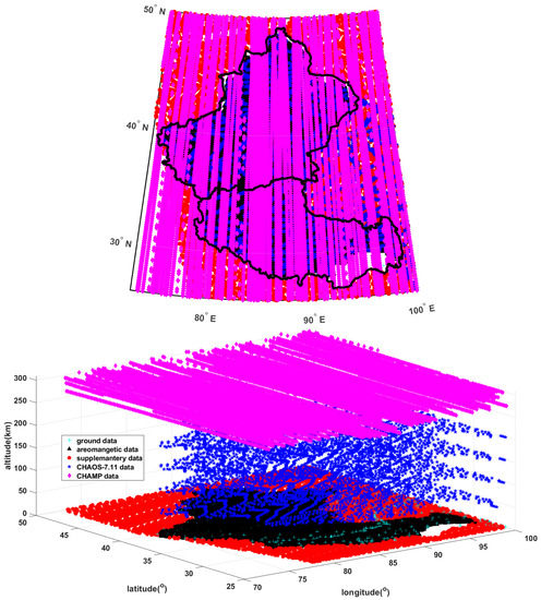
Figure 1.
All 34039 data points over Xinjiang and Tibet are distributed in 2D (top) and 3D (bottom) views. Lambert conformal projection.
3. Modeling Methods
3.1. Three-Dimensional Surface Spline Model
Based on the 2DSS model [17], Feng et al. [20] added an altitude term and obtained the three-dimensional Surface Spline (3DSS) model. The expressions are as follows:
where is a geomagnetic component; refer to latitude, longitude, and altitude, respectively; ; is the number of data; and are undetermined coefficients; are the latitudes, longitudes, and altitudes of all measuring points; and is a small value that controls the changes on the surface curvature and is generally chosen as 1 × 10⁻⁷.
The coefficients can finally be calculated by the Gaussian elimination method, , where n is the number of measuring points, and are coefficients.
3.2. Regional Spherical Harmonic Analysis Model
The Regional Spherical Harmonic Analysis (RSHA) model is based on a depleted basis of the global spherical harmonic function [36]. We focus on the lithospheric field over Xinjiang, which can be seen as a spheric cap, so the eigenvalues through Gauss coefficients are used to calculate the new coefficients that only work in the research area. Due to the uneven distribution of measuring data, we suppose the magnetic field is
where is the magnetic field, is the spherical harmonic series of the cap, and is a vector of coefficients; thus, a normal equation can be obtained, and its eigenvectors are .
Two simplified methods, the three largest eigenvalues, and the basis function’s symmetry simplify the calculation and enable the calculation to be much simpler. By transforming the spherical cap coordinate, the residuals E can be followed as
where are kernels matrices, are new coordinate system vectors, are errors, and new coefficients that are given by eigenvectors. The new Gauss coefficients can then be finally derived by
by which the resulting RSH model suitable for Xinjiang can be obtained.
Coefficients m comes from the classical spherical harmonic function
where are radial distance, co-latitude, longitude, and time; a is the reference radius of the Earth (a = 6371.2km); are Gauss coefficients; and is the Schmidt semi-normalized associated Legendre function of degree n and order m.
3.3. Other Models
Besides the two regional 3D models, the global magnetic models, SHA1000, LCS-1, and NGDC720, with higher truncation degrees, are also adopted for verification and comparison.
Thébault et al. [13] derived a global magnetic field model based on Swarm, CHAMP, WDMAM-2 grids, and the R-SCHA model. They converted this regional model into the global model with SH degree 1050 and obtained an excellent consistency with previous models. They paid more attention to the anomalies over the South Atlantic Anomaly (SAA) and found the sign’s change in the secular acceleration of element Z on the Pacific Ocean. The LCS-1 model was derived only from satellite data [12], with coefficients that are the as same as CHAOS-7 while N > 25. The NGDC720 [9] with a degree of 720 is also used for comparison. This model was derived by the National Geophysical Data Center (NGDC) of the United States by combining data from satellite, ground, oceanic, and aeromagnetic surveys.
4. Modeling Results
4.1. Comparison between Different Models
The investigations are all about the total intensity F throughout the article. After inversion and forward modeling, the 3DSS and RSHA model with degree 400 (RSHA400) that correspond to resolutions with 0.01° (about 1.11 km) are derived. We list the lithospheric field distributions based on different numbers of measuring data and models at the 1km altitude (Figure 2); they have the same color bar.
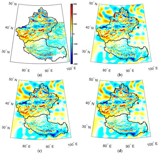
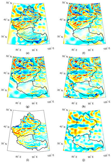
Figure 2.
The lithospheric field distribution over Xinjiang and Tibet based on different models. Units: nT. (a) Original aeromagnetic data; (b) 3DSS20678; (c) 3DSS24239; (d) 3DSS29776; (e) 3DSS34039; (f) SHA1000; (g) SHA720; (h) NGDC720; (i) RSHA400; (j) LCS−1.
All the figures show similar fundamental trends inside the research area. According to Figure 2a–e, the distributions of 3DSS with different data numbers look consistent and highly identical to the original aeromagnetic distribution. The more modeling data there is, the more details each figure reflects, particularly in the north and east parts of Xinjiang and the south-positive stripe of Tibet. Regarding the other models, it is obvious that the higher the degree of the model is, the more details it has; RSHA400 looks much simpler than SHA1000 and only reflect the medium-scale part of the magnetic field. Nevertheless, the LCS-1 model is the simplest because it is only 185 degrees and corresponds to a large scale of about 216 km. In addition, the distributions of the 3DSS model nearby and outside the boundary are not continuous, so we added supplementary points to alleviate this situation. The main reason is the need for measuring data outside the Chinese boundary; however, the four other models were derived by measuring data worldwide.
4.2. Comparison of the 3DSS Model at Different Altitudes
Here, we model the lithospheric field from 0 km to 2.0 km in intervals of 0.1 km, and list them in Figure 3, they have the same color bar. The densest data are aeromagnetic data at 1 km.
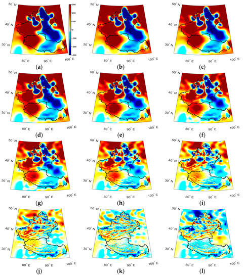
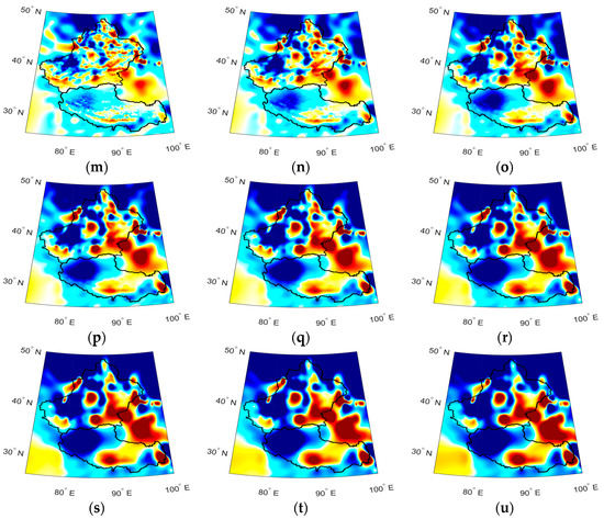
Figure 3.
The lithospheric field distribution over Xinjiang and Tibet based on 3DSS34039 at different altitudes. Units: nT. (a–u): 0, 0.1, 0.2, …, 2.0 km.
Figure 3a–h show the consistent and straightforward structures due to the unevenly distributed grounded data from 0 to 0.7 km. The number of grounded data is 519 and accounts for only 1.52%. With the increases in altitude and the number of modeling points, the distributions gradually show more details of the middle- and small-scale magnetic fields. There are 12,511 aeromagnetic points at 1.0 km (Figure 3k), accounting for 36.75%, especially in the north and east of Xinjiang and the south of Tibet. From Figure 3l, The number of points gradually decreases, and the distribution becomes simple and almost fixed since Figure 3p. This decrease is because of the modeling data being rapidly decreased, and there was a lack of control in the redial direction. Some anomalies rapidly change its intensity, such as the positive anomaly in the southwestern Xinjiang, and the negative anomaly in the southeastern Tibet. This means the distributions could be more reliable due to the uneven data coverage in a radial direction.
In order to verify the result, we calculate the lithospheric field by using only 519 pieces of ground data and compare it with the 3DSS model at 0 km. Two distributions are shown is Figure 4.
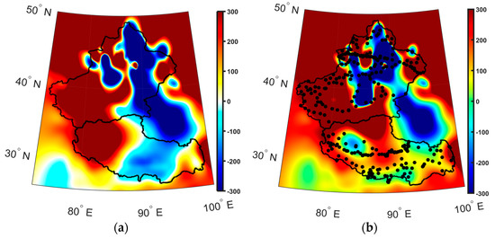
Figure 4.
The comparison of the lithospheric field at 0 km level. Units: nT. (a) 3DSS34039; (b) 3DSS only based on 519 pieces of ground data. ●: ground points.
After careful comparison, there are some differences between the two models, especially in the western part of Tibet, which shows a small negative area of the ground data model. In contrast, there is only a positive part of the 3DSS model; part of the reason is that the points in the Qinghai−Tibet Plateau are around 4 km. Hence, the exact distribution is negative and different from the distribution at 0 km by the 3DSS model. However, the total distributions of the two figures are similar, particularly in the negative part that crosses Xinjiang and Tibet and the positive part in the western parts of Xinjiang. Thus, this comparison shows that the new model is reliable.
4.3. Error Analysis
4.3.1. Comparison of Different Distributions
We calculate and illustrate the difference figures among the 3DSS34039, SHA1000, and NGDC720 models in Figure 5 to test the modeling error and to inspect the differences.
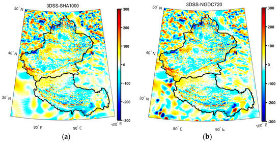
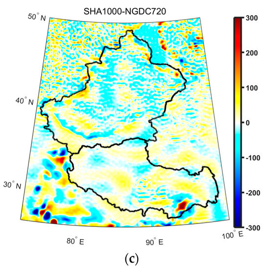
Figure 5.
The total field difference distribution of lithospheric field distribution among 3DSS34039, SHA1000, and NGDC720 models. Units: nT. (a) 3DSS−SHA1000; (b) 3DSS−NGDC720; (c) SHA1000− NGDC720.
The differences between 3DSS34039 and the other two models (Figure 5a,b) are highly consistent, except for several large anomalies in central Xinjiang; the northern, eastern, and western parts of Xinjiang; and the southern part of Tibet. However, the difference between SHA1000 and NGDC720 is minimal, which means the 3DSS model reflects more lithospheric details than the other models and illustrates the regional model’s advantages based on the dense-enough measuring data. Due to the lack of data in the southeast part of Tibet, the significant anomaly is unreliable.
4.3.2. Error Test
Due to the modeling theory of 3DSS, we abstract 11 3DSS modeling points (Figure 6), one grounded, three aeromagnetic, one supplementary, three CHAOS, and three CHAMP points, randomly according to the percentage of data and then derive the models based on the rest of the data (34,028, 29,765, 24,228, and 20,676 points). Finally, we forward predicted these 11 points to check the RMSE in Figure 7 and Table 2.
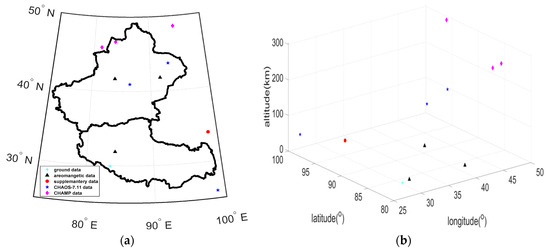
Figure 6.
The distribution of 11 absent points in 2D (a) and 3D (b) views.
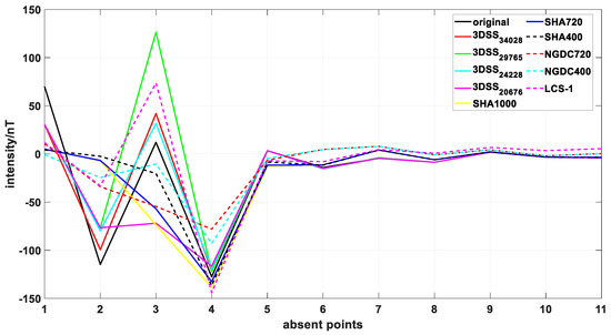
Figure 7.
The comparison of all predicted absent points based on different models.
Table 2.
The RMSE values of 11 absent points based on different models.
5. Geological Interpretation
The Xinjiang–Tibet area is mainly comprised of plateaus, mountains, and basins. This is the highest area of China, particularly in the Qinghai Tibet Plateau, which is at an elevation greater than 4 km. The study area has a kidney shape. We analyzed the Xinjiang and Tibet geological structures and lithospheric fields separately. Xinjiang is located in the hinterland of Eurasia, and the geographical range is 73°40′E–96°18′E, 34°25′N–48°10′N. The mountains and basins are arranged alternately. The basins and mountains are surrounded by each other, known as three mountains with two basins. The Altai Mountains are in the north, and the Kunlun Mountains are in the south; the Tianshan Mountains stretch across the central part of Xinjiang, dividing Xinjiang into two halves: the Tarim Basin in the south and the Junggar Basin in the north. This geomorphic feature also roughly reflects the paleo-tectonic pattern of the lithosphere. The mountains are mainly composed of paleo-continental margins and collision zones, and the basin is a subsided ancient land block. Here, we chose 3DSS and SHA1000 as an example (Figure 8) to analyze.
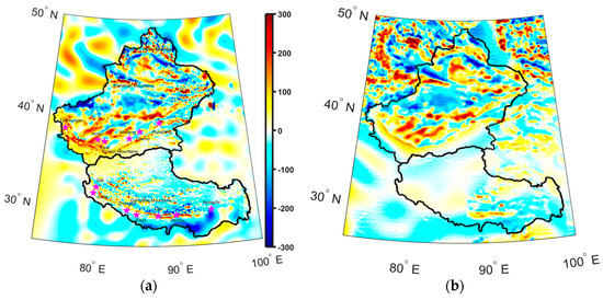
Figure 8.
The distribution of lithospheric field based on 3DSS34039 (a) and SHA1000 (b) models. Units: nT.
There are four obvious magnetic anomalies inside Xinjiang: The South Tarim magnetic anomaly, the Turpan–Hami magnetic anomaly, the Altai magnetic anomaly, and the Yili magnetic anomaly. They have good correspondence with the local structures. The consistency between the positive magnetic anomaly stripe in southwest Xinjiang and its neighboring Tashkurgan–Hotan–Cele–Minfeng–Qiemo–Ruoqiang belt (the pink stars in Figure 8a) and the middle edge of the Kunlun Mountains is the most apparent difference between 3DSS and the other models, especially the highest degree model, SHA1000. The stripe can be separated into the Western Kunlun folded belt and the Eastern Kunlun orogenic belt, forming a big lower convex arc belt anomaly. The western part of the stripe was formed in the late Early Permian, accompanied by a large number of acid magma intrusions, a Devonian sandy conglomerate, and medium and acid volcanic rocks covering the eastern part [21,23]. The sedimentary characteristics of the upper Paleozoic are consistent with those in the Qaidam block to the north, and they all belong to platform-type shallow marine facies. The desert covers the surface in the fourth quarter, so the magnetic field source is shallow, generally around 2–3 m. It is speculated that the anomaly distributed along the NE belt is related to magnetic intrusions. It is further implied that there may be a large deep fault zone beneath the middle edge of the Kunlun Mountains, and these magnetic intrusions are distributed along the fault zone.
Tibet is dominated by the plateau, composed of huge mountains and plateaus inlaid with wide valleys and basins. The geographical range is 78°25′E–99°06′E, 26°50′N–36°53′N. Repeated tectonic movements formed the plateau landform during the geological period [42]. The geological structures in Tibet are mainly Yanshan and Himalayan folds, while the rocks are mainly Himalayan basalt. Compared with Xinjiang, the lithosphere distribution in Tibet is much weaker, and the strong magnetic field is mainly distributed in southern Tibet. Compared with SHA1000, the 3DSS model can reflect more details of the lithospheric magnetic field (Figure 8).
Compared to the SHA model, the 3DSS model depicts a typical positive magnetic anomaly belt in southern Tibet that runs from northwest to southeast, starting in Gar County and continuing along Zhada, Zhongba, Saga, Lazi, Renbu, and near Nyingchi (the pink stars in Figure 8). Additionally, there is a positive and negative interlaced magnetic anomaly area near Lhasa City. Positive and negative magnetic anomaly points (29°24′N, 90°16′E) with absolute value intensity exceeding 400 nT have appeared near Renbu. In addition, some positive and negative magnetic anomalies have also appeared in central Ali and southeast Naqu, where the extreme value intensity exceeds 300 nT. The positive magnetic anomaly stripe distribution is considered highly consistent with the Gangdise Mountains, by comparing the geological structures.
The positive anomaly from the Lhasa massif and the negative anomaly from the Himalayan massif are surrounded by large orogenic belts such as the Himalayas, Longmen Mountains, Daba Mountains, etc., consistent with the results of Kang et al. [31]. The magnetic anomaly is less strong than in Tarim, Xinjiang. This shows that the orogenic terrain and the magnetic minerals in the shallow lithospheric field mainly cause it. The source of the lithospheric magnetic field is shallow, which also shows that the magnetic field strength has little relationship with the thickness of the crust.
6. Comparison between the Lithospheric Field and the Surface Heat Flow
We inspected and extracted the measuring points of the heat flow over the study area to find out the relationship between the surface heat flow and the regional lithospheric field over the study area and first list the classification of the heat flow (Figure 9).
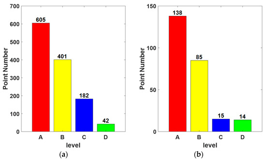
Figure 9.
The level of heat flow points over China (a) and over Xinjiang and Tibet area (b).
There are 1230 heat flow points in China. After carefully inspecting the data and finally obtaining the 252 points in the Xinjiang and Tibet area, the data quality is divided into A, B, C, and D levels, which denote very good, good, normal, and less good, respectively. Thus, the good data account for 88.5%, which shows that the modeling is reliable.
We illustrate the distribution of the heat flow based on measuring points and the distribution by the 2D Surface Spline (2DSS) model (the altitudes of all points are very close), which shows more details with a higher resolution (0.1°); the whole mainland’s distribution by Hu is also listed (Figure 10) for verification.
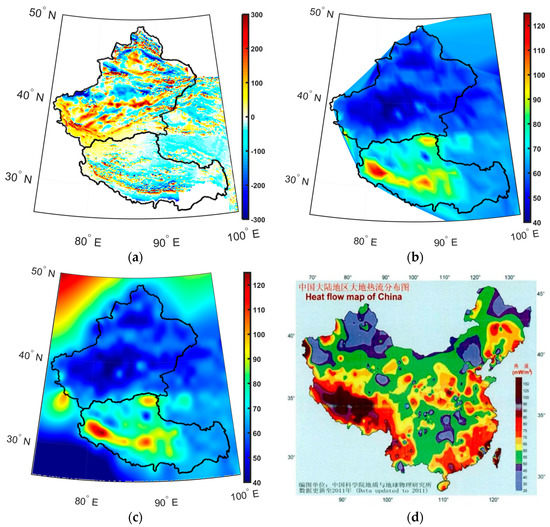
Figure 10.
The comparison between lithospheric field and heat flow. Units: nT and mW/m2. (a) the distribution of the lithospheric field based on 3DSS34039; (b) the heat flow based on the origin measuring points; (c) the heat flow based on the 2DSS model; (d), the heat flow over the Chinese mainland. Mapping department: Institute of Geology and Geophysics, Chinese Academy of Sciences [35].
All parameters are consistent with Equations (1) and (2).
The figures above show the distributions of heat flow based only on points (Figure 10b), and the model (Figure 10c) is highly consistent, which implies that the 2DSS model is reliable and consistent with the same areas of Figure 10d derived by Hu [35]. The intensity in Tibet is higher than that in Xinjiang, the intensity in Qinghai–Tibet Plateau is greater than 80 mW/ m2, and there is a big positive anomaly around 125 mW/m2 nearby Zada and a negative anomaly around 50 mW/m2 at 33.7°N, 87.9°E.
After comparing with Figure 10a, the positive heat flow stripe coincides with the lithospheric field’s positive stripe in southern Tibet. A northward negative part corresponds to the same sign part of the lithospheric field. However, the correlation in Xinjiang needs to be clarified, and there is no obvious heat flow variation.
The corners in Figure 10c show a strong boundary effect. The main reason is the need for measuring points outside the research area, or serious distortions of forward modeling are generated.
7. Conclusions
We chose ground, airborne, and CHMAP satellite data to create the lithospheric magnetic field models using 3DSS and RSHA models. The external and core parts were removed from the measuring data. The results were compared with the original measuring data and the LCS-1, NGDC-720, and SHA1000 models. In addition, we checked the variation of the field along the altitude, the possible relationship between the magnetic field and geological structure, and the surface heat flow. Finally, several conclusions were reached as follows:
1. The 3DSS model can excellently model the spatially lithospheric field and illustrate more details than other regional and global models. The main reason is that the 3DSS model is good at modeling complicated magnetic fields, and the relatively good spatial distribution of the modeling points can provide coverage in the horizontal and vertical directions. The model is robust due to no obvious artificial anomalies being yielded, even with the fewest modeling points compared to the original data.
2. Some new characteristics can be seen in the new model, such as the consistency between the positive anomaly stripe in southwest Xinjiang and its neighboring Tashkurgan–Hotan–Cele–Minfeng–Qiemo–Ruoqiang belt and the middle edge of the Kunlun Mountains. The stripe has a shallow magnetic field source and is related to magnetic intrusions; the lithospheric field in Tibet is weaker.
These findings imply that the orogenic terrain of mountains and the magnetic minerals in the shallow crust mainly cause the lithospheric field’s formation. The source of the lithospheric magnetic field is relatively shallow, implying that the magnetic field strength has little relationship with the thickness of the crust.
3. Compared with the surface heat flow, there is a good consistency between a positive stripe of heat flow and a positive stripe of the lithospheric field in southern Tibet. The high heat flow areas correspond to the low intensity of the lithospheric field, and vice versa, in Xinjiang, particularly in the south Tarim Basin and Junggar Basin magnetic anomalies. The big heat flow values might be linked with the shallow Curie surface. Gao et al. [26] suggested that the topography of the Curie surface corresponds to the heat flow values well. The high heat flow occurs in the basement where the surface is shallow, and vice versa. Due to the rock composition, the shallow Curie surface denotes the demagnetization process close to the surface. However, more ferromagnetic minerals, Titanium magnetite, are increased there, such as the Kursk magnetic anomaly in Russia. The strong heat flows in the Tibetan Plateau are still unclear and might be caused by over-modeling or the fewer measuring points.
The new 3DSS model shows its advantages for modeling the regional lithospheric magnetic field, particularly in small-scale regions, and then provides an idea reference to study the possible formation and variation of such a field. However, a few things from the modeling still deserve to be seriously considered: the precise extraction of the lithospheric field from the raw data, the denser modeling data along the radial direction, and the better supplementary data outside the boundary, such as the marine measuring data. The correspondence mechanism between the lithospheric field and heat flow may draw more attention.
Soon, the coming geomagnetic satellite, Macau Science Satellite-1 (MSS-1), will provide higher quality and revolutionary low inclination (±41° near the west–east direction) measuring data, which must be helpful to derive a better regional lithospheric magnetic field model.
Author Contributions
Conceptualization, Y.F. and Y.H.; methodology, Y.F.; software, Y.L. and J.Z. (Jinyuan Zhang); validation, J.Z. (Jiaxuan Zhang); writing—original draft preparation, Y.F.; writing—review and editing, A.N.; supervision, Y.F.; funding acquisition, Y.F. All authors have read and agreed to the published version of the manuscript.
Funding
This research was funded by the National Natural Science Foundation of China (Nos. 42250103, 41974073, and 41404053), the Macau Foundation and the pre-research project of Civil Aerospace Technologies (Nos. D020308 and D020303), and the Specialized Research Fund for State Key Laboratories.
Data Availability Statement
CHAOS-7.11 is available at http://www.spacecenter.dk/files/magnetic-models/CHAOS-7/ (accessed on 11 December 2022); LCS-1 is available at http://www.spacecenter.dk/files/magnetic-models/LCS-1/ (accessed on 17 December 2022); and NGDC720 is available at https://geomag.us/models/ngdc720.html (accessed on 11 December 2022). All measuring data are available upon request.
Acknowledgments
The authors would like to thank the reviewers for their constructive comments and suggestions.
Conflicts of Interest
The authors declare no conflict of interest.
References
- Olsen, N.; Hulot, G.; Sabaka, T.J. Geomagnetism. In Treatise in Geophysics; Schubert, G., Ed.; Elsevier Ltd.: Amsterdam, The Netherlands, 2007; Volume 5, pp. 33–75. [Google Scholar]
- Reigber, C.; Lühr, H.; Schwintzer, P. Champ Mission status. Adv. Space Res. 2002, 30, 129–134. [Google Scholar] [CrossRef]
- Friis-Christensen, E.; Lühr, H.; Hulot, G. Swarm: A constellation to study the Earth’s magnetic field. Earth Planets Space 2006, 58, 351–358. [Google Scholar] [CrossRef]
- Sabaka, T.J.; Olsen, N.; Purucker, M.E. Extending comprehensive models of the Earth’s magnetic field with Ørsted and Champ data. Geophys. J. Int. 2004, 159, 521–547. [Google Scholar] [CrossRef]
- Sabaka, T.J.; Olsen, N.; Tyler, R.H.; Kuvshinov, A. CM5, a pre-Swarm comprehensive geomagnetic field model derived from over 12 yr of CHAMP, Ørsted, SAC-C and observatory data. Geophys. J. Int. 2015, 200, 1596–1626. [Google Scholar] [CrossRef]
- Sabaka, T.J.; Toffner-Clausen, L.; Olsen, N.; Finlay, C.C. CM6: A comprehensive geomagnetic field model derived from both CHAMP and Swarm satellite observations. Earth Planets Space 2020, 72, 80. [Google Scholar] [CrossRef]
- Finlay, C.C.; Olsen, N.; Kotsiaros, S.; Gillet, N.; Tøffner-Clausen, L. Recent geomagnetic secular variation from Swarm and ground observatories as estimated in the CHAOS-6 geomagnetic field model. Earth Planets Space 2016, 68, 112. [Google Scholar] [CrossRef]
- Finlay, C.C.; Kloss, C.; Olsen, N.; Hammer, M.D.; Toffner-Clausen, L.; Grayver, A.; Kuvshinov, A. The CHAOS-7 geomagnetic field model and observed changes in the South Atlantic Anomaly. Earth Planets Space 2020, 72, 156. [Google Scholar] [CrossRef]
- Maus, S. An ellipsoidal harmonic representation of Earth’s lithospheric magnetic field todegree and order 720. Geochem. Geophys. Geosyst. 2010, 11, Q06015. [Google Scholar] [CrossRef]
- Maus, S.; Yin, F.; Lühr, H.; Manoj, C.; Rother, M.; Rauberg, J.; Stolle, C.; Müller, R.D. Resolution of direction of oceanic magnetic lineation by the sixth—Generation lithospheric magnetic field model from CHAMP satellite magnetic measurements. Geochem. Geophys. Geosyst. 2008, 9, Q07021. [Google Scholar] [CrossRef]
- Maus, S. Magnetic Field Model MF7. Available online: https://www.geomag.us/models/MF7.html (accessed on 10 October 2022).
- Olsen, N.; Ravat, D.; Finlay, C.C.; Kother, L.K. LCS-1: A highresolution global model of the lithospheric magnetic field derived from CHAMP and Swarm satellite observations. Geophys. J. Int. 2017, 211, 1461–1477. [Google Scholar] [CrossRef]
- Thébault, E.; Hulot, G.; Langlais, B.; Vigneron, P. A spherical harmonic model of Earth’s lithospheric magnetic field up to degree 1050. Geophys. Res. Lett. 2021, 48, e2021GL095147. [Google Scholar] [CrossRef]
- Le Mouel, J. Sur la Distribution des Elements Magnetiques en France. Ph.D. Thesis, University de Paris, Paris, France, 1969. [Google Scholar]
- Haines, G.V. Spherical cap harmonic analysis. J. Geophys. Res. 1985, 90, 2583–2592. [Google Scholar] [CrossRef]
- Thébault, E.; Schott, J.J.; Mandea, M. Revised spherical cap harmonic analysis (R-SCHA): Validation and properties. J. Geophys. Res. 2006, 111, B01102. [Google Scholar] [CrossRef]
- An, Z.C.; Xu, Y.F. Methods of computation of geomagnetic field at greater altitude in a local region. Chin. J. Space Sci. 1981, 1, 68–73. [Google Scholar] [CrossRef]
- Alldredge, L.R. Rectangular harmonic analysis applied to the geomagnetic field. J. Geophys. Res. 1981, 86, 3021–3026. [Google Scholar] [CrossRef]
- Liu, S.J.; Zhou, X.G.; Sun, H.; An, Z.C. The three dimension Taylor polynomial method for the calculation of regional geomagnetic field model. Prog. Geophys. 2011, 26, 1165–1174. [Google Scholar] [CrossRef]
- Feng, Y.; Jiang, Y.; Sun, H.; An, Z.C.; Huang, Y. The three-dimensional surface Spline model of geomagnetic field. Chin. J. Geophys. 2018, 61, 1352–1365. [Google Scholar] [CrossRef]
- Tu, G.Z.; He, G.Q.; Xu, X.; Li, J.Y.; Hao, J.; Cheng, S.D.; Deng, Z.Q.; Li, Y.A. Crustal Structure and Geological Evolution in Xinjiang, China; Geological Press House: Beijing, China, 2010. (In Chinese) [Google Scholar]
- Yang, F.X.; Chen, B.; Yang, X.; Zheng, L.M.; Sun, H.J.; Paerhati, Z. Analysis on the data derived from the mobile magentic repeat survey in the KASHIWUQIA region. Inland Earthq. 2010, 24, 352–358. [Google Scholar]
- Ding, X.J.; Yang, F.X.; Jia, L.; Wang, C. Analysis of Local lithospheric magnetic field anomalies characteristics before Xinjiang Pishan Ms6.5 Earthquake in 2015. J. Seismol. Res. 2017, 40, 362–367. [Google Scholar]
- Chen, L.; Liu, D.Q.; Li, J.; Ailixiati, Y.S.; Li, G.R.; Li, R.; Ding, X.J.; Sun, X.X. Mobile magnetic and gravity survey in Kashi and its adjacent regions. Technol. Earthq. Disater Prev. 2017, 12, 423–432. [Google Scholar]
- Gao, G.M.; Kang, G.F.; Bai, C.H.; Li, G.Q. Distribution of the crustal magnetic anomaly and geological structure in Xinjiang, China. J. Asian Earth Sci. 2013, 77, 12–20. [Google Scholar] [CrossRef]
- Gao, G.M.; Kang, G.F.; Li, G.Q.; Bai, C.H. Crustal magnetic anomaly and Curie surface beneath Tarim. Basin, China, and its adjacent area. Can. J. Earth Sci. 2015, 52, 357–367. [Google Scholar] [CrossRef]
- Zhao, J.M.; Chen, S.Z.; Zhang, H.; Liu, H.B.; Shao, X.Z.; Chen, X.F.; Xu, J.; Ma, Z.J. Lithospheric structure beneath the eastern Junggar Basin (NW China), inferred from velocity, gravity and geomagnetism. J. Asian Earth Sci. 2019, 177, 295–306. [Google Scholar] [CrossRef]
- Zhang, C.D. The magnetic characteristics of crust beneath Xizhang (Tibetan) plateau deduced from satellite magnetic anomaly. Prog. Geophys. 2002, 17, 325–330. [Google Scholar]
- Wang, Y.H. The investigation of geomagnetic field in Qinhai Xizang plateau. Prog. Geophys. 1998, 13, 45–51. [Google Scholar]
- An, Z.C. Studies on geomagnetic field models of Qinhai-Xizang Plateau. Chin. J. Geophys. 2000, 43, 339–345. [Google Scholar] [CrossRef]
- Kang, G.F.; GAO, G.M.; BAI, C.H.; SHAO, D.; FENG, L.L. Characteristics of the crustal magnetic anomaly and regional tectonics in the Qinghai-Tibet Plateau and the adjacent areas. Sci. China Earth Sci. 2012, 55, 1028–1036. [Google Scholar] [CrossRef]
- Ten, J.W. Lithospheric Physics and Dynamics of Kangdian Tectonic Belt; Science Press: Beijing, China, 1994. (In Chinese) [Google Scholar]
- Ou, J.M.; Du, A.M.; Thébault, E.; Xu, W.Y.; Tian, X.B.; Zhang, T.L. A high resolution lithospheric magnetic field model over China. Sci. China Earth Sci. 2013, 56, 1759–1768. [Google Scholar] [CrossRef]
- Wen, L.M.; Kang, G.F.; Bai, C.H.; Gao, G.M. Studies on the relationships of the Curie surface with heat flow and crustal structures in Yunnan Province, China, and its adjacent areas. Earth Planets Space 2019, 71, 85. [Google Scholar] [CrossRef]
- Hu, S.B.; He, L.J.; Wang, J.Y. Heat flow in the continental area of China: A new data set. Earth Planet Sci. Lett. 2000, 179, 407–419. [Google Scholar] [CrossRef]
- Jiang, Y.; Holme, R.; Xiong, S.Q.; Jiang, Y.; Feng, Y.; Yang, H. Long-wavelength lithospheric magnetic field of China. Geophys. J. Int. 2021, 224, ggaa490. [Google Scholar] [CrossRef]
- Alken, P.; Thebault, E.; Beggan, C.D.; Amit, H.; Aubert, J.; Baerenzung, J.; Bondar, T.N.; Brown, W.J.; Califf, S.; Chambodut, A.; et al. International Geomagnetic Reference Field: The thirteenth generation. Earth Planets Space 2021, 73, 49. [Google Scholar] [CrossRef]
- Xiong, S.Q.; Tong, J.; Ding, Y.Y.; Li, Z.K. Aeromagnetic data and geological structure of continental China: A review. Appl. Geophys. 2016, 13, 227–237. [Google Scholar] [CrossRef]
- Wang, J.Y.; Huang, S.P. Compilation of heat flow data in the China continental area (2nd Edition). Seimilogy Geol. 1990, 12, 351–366. [Google Scholar]
- Hu, S.B.; He, L.J.; Wang, J.Y. Compilation of heat flow data in the China continental area (3rd edition). Chin. J. Geophys. 2001, 49, 745–752. [Google Scholar] [CrossRef]
- Jiang, G.Z.; Gao, P.; Rao, S.; Zhang, L.; Tang, X.; Huang, F.; Zhao, P.; He, L.; Hu, S.; Wang, J.; et al. Compilation of heat flow data in the China continental area (4th edition). Chin. J. Geophys. 2016, 59, 2892–2910. [Google Scholar] [CrossRef]
- Yang, Y.C.; Li, B.Y.; Yi, Z.S.; Zhang, Q.S. The formation and evolution of landforms in the Xizang plateau. Acta Geophys. Sin. 1982, 37, 76–87. [Google Scholar]


Disclaimer/Publisher’s Note: The statements, opinions and data contained in all publications are solely those of the individual author(s) and contributor(s) and not of MDPI and/or the editor(s). MDPI and/or the editor(s) disclaim responsibility for any injury to people or property resulting from any ideas, methods, instructions or products referred to in the content. |
© 2023 by the authors. Licensee MDPI, Basel, Switzerland. This article is an open access article distributed under the terms and conditions of the Creative Commons Attribution (CC BY) license (https://creativecommons.org/licenses/by/4.0/).