

Geomatic Data Fusion for 3D Tree Modeling: The Case Study of Monumental Chestnut Trees
 , , , ,
  and
and 
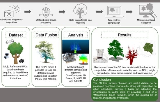
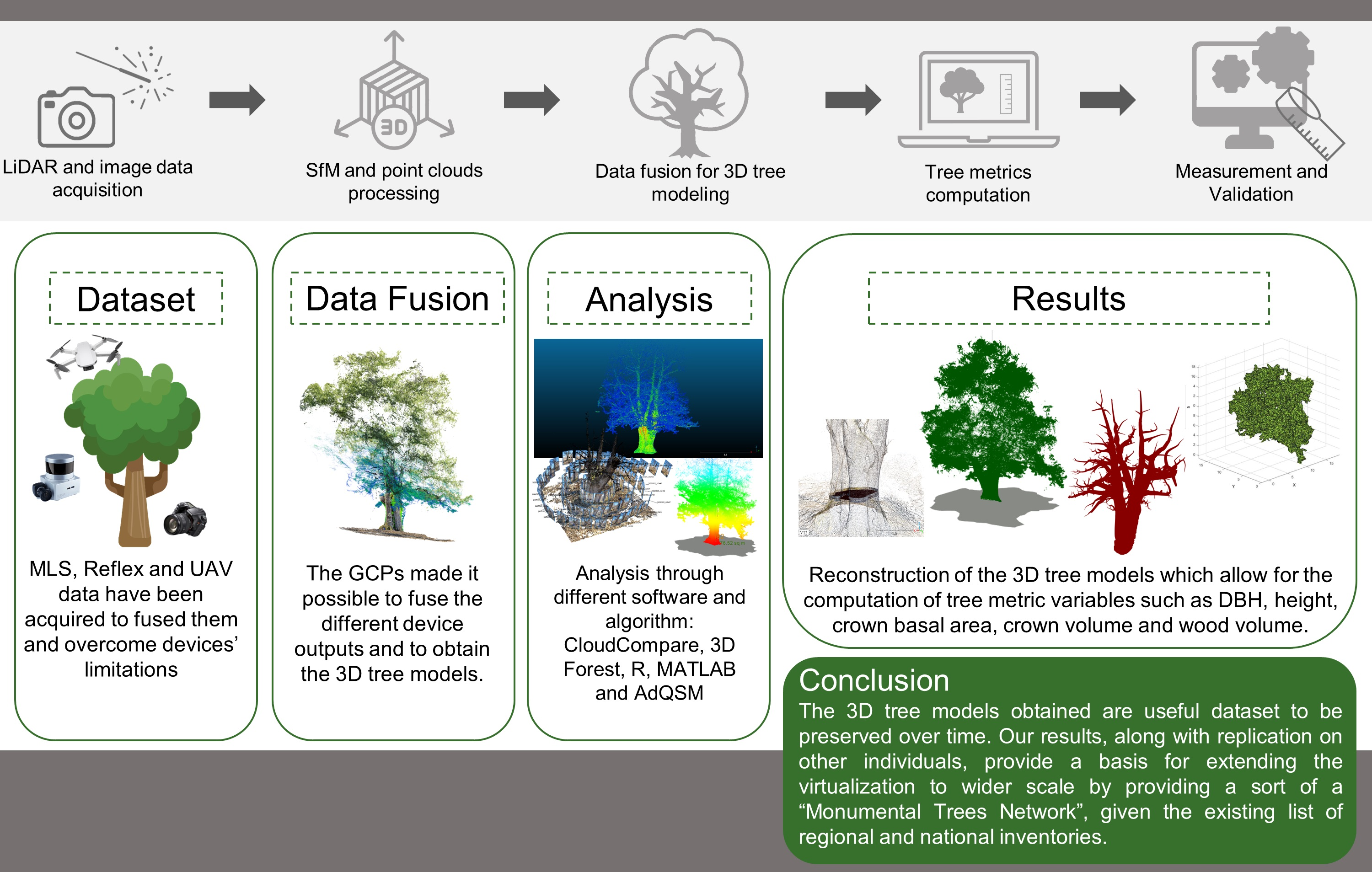
Abstract
1. Introduction
2. Materials and Methods
2.1. Monumental Tree Locations and Features
2.2. Geomatic Devices Surveys
2.3. Point Clouds Processing
3. Results
3D Models and Tree Metrics Data Extraction
4. Discussion
5. Conclusions
Author Contributions
Funding
Data Availability Statement
Acknowledgments
Conflicts of Interest
References
- Di Stefano, F.; Chiappini, S.; Gorreja, A.; Balestra, M.; Pierdicca, R. Mobile 3D scan LiDAR: A literature review. Geomat. Nat. Hazards Risk 2021, 12, 2387–2429. [Google Scholar] [CrossRef]
- Boccardo, P.; Giulio Tonolo, F. Remote sensing role in emergency mapping for disaster response. In Engineering Geology for Society and Territory-Volume 5: Urban Geology, Sustainable Planning and Landscape Exploitation; Springer: Berlin/Heidelberg, Germany, 2015; pp. 17–24. [Google Scholar]
- Dechesne, C.; Mallet, C.; Le Bris, A.; Gouet-Brunet, V. Semantic segmentation of forest stands of pure species combining airborne lidar data and very high resolution multispectral imagery. ISPRS J. Photogramm. Remote Sens. 2017, 126, 129–145. [Google Scholar] [CrossRef]
- Apostol, B.; Petrila, M.; Lorenţ, A.; Ciceu, A.; Gancz, V.; Badea, O. Species discrimination and individual tree detection for predicting main dendrometric characteristics in mixed temperate forests by use of airborne laser scanning and ultra-high-resolution imagery. Sci. Total Environ. 2020, 698, 134074. [Google Scholar] [CrossRef] [PubMed]
- Hościło, A.; Lewandowska, A. Mapping forest type and tree species on a regional scale using multi-temporal Sentinel-2 data. Remote Sens. 2019, 11, 929. [Google Scholar] [CrossRef]
- Lang, N.; Kalischek, N.; Armston, J.; Schindler, K.; Dubayah, R.; Wegner, J.D. Global canopy height regression and uncertainty estimation from GEDI LIDAR waveforms with deep ensembles. Remote Sens. Environ. 2022, 268, 112760. [Google Scholar] [CrossRef]
- Potapov, P.; Li, X.; Hernandez-Serna, A.; Tyukavina, A.; Hansen, M.C.; Kommareddy, A.; Pickens, A.; Turubanova, S.; Tang, H.; Silva, C.E. Mapping global forest canopy height through integration of GEDI and Landsat data. Remote Sens. Environ. 2021, 253, 112165. [Google Scholar] [CrossRef]
- Ghamisi, P.; Rasti, B.; Yokoya, N.; Wang, Q.; Hofle, B.; Bruzzone, L.; Bovolo, F.; Chi, M.; Anders, K.; Gloaguen, R. Multisource and multitemporal data fusion in remote sensing: A comprehensive review of the state of the art. IEEE Geosci. Remote Sens. Mag. 2019, 7, 6–39. [Google Scholar] [CrossRef]
- Zhang, J.; Lin, X. Advances in fusion of optical imagery and LiDAR point cloud applied to photogrammetry and remote sensing. Int. J. Image Data Fusion 2017, 8, 1–31. [Google Scholar] [CrossRef]
- Suwardhi, D.; Fauzan, K.N.; Harto, A.B.; Soeksmantono, B.; Virtriana, R.; Murtiyoso, A. 3D Modeling of Individual Trees from LiDAR and Photogrammetric Point Clouds by Explicit Parametric Representations for Green Open Space (GOS) Management. ISPRS Int. J. Geo-Inf. 2022, 11, 174. [Google Scholar] [CrossRef]
- Cao, L.; Liu, H.; Fu, X.; Zhang, Z.; Shen, X.; Ruan, H. Comparison of UAV LiDAR and digital aerial photogrammetry point clouds for estimating forest structural attributes in subtropical planted forests. Forests 2019, 10, 145. [Google Scholar] [CrossRef]
- Tupinambá-Simões, F.; Pascual, A.; Guerra-Hernández, J.; Ordóñez, C.; de Conto, T.; Bravo, F. Assessing the Performance of a Handheld Laser Scanning System for Individual Tree Mapping—A Mixed Forests Showcase in Spain. Remote Sens. 2023, 15, 1169. [Google Scholar] [CrossRef]
- Liu, Q.; Li, S.; Li, Z.; Fu, L.; Hu, K. Review on the applications of UAV-based LiDAR and photogrammetry in forestry. Sci. Silvae Sin. 2017, 53, 134–148. [Google Scholar]
- Lian, X.; Zhang, H.; Xiao, W.; Lei, Y.; Ge, L.; Qin, K.; He, Y.; Dong, Q.; Li, L.; Han, Y. Biomass Calculations of Individual Trees Based on Unmanned Aerial Vehicle Multispectral Imagery and Laser Scanning Combined with Terrestrial Laser Scanning in Complex Stands. Remote Sens. 2022, 14, 4715. [Google Scholar] [CrossRef]
- Qi, Y.; Coops, N.C.; Daniels, L.D.; Butson, C.R. Comparing tree attributes derived from quantitative structure models based on drone and mobile laser scanning point clouds across varying canopy cover conditions. ISPRS J. Photogramm. Remote Sens. 2022, 192, 49–65. [Google Scholar] [CrossRef]
- Qi, Y.; Coops, N.C.; Daniels, L.D.; Butson, C.R. Assessing the effects of burn severity on post-fire tree structures using the fused drone and mobile laser scanning point clouds. Front. Environ. Sci. 2022, 10, 1362. [Google Scholar] [CrossRef]
- Pyörälä, J.; Saarinen, N.; Kankare, V.; Coops, N.C.; Liang, X.; Wang, Y.; Holopainen, M.; Hyyppä, J.; Vastaranta, M. Variability of wood properties using airborne and terrestrial laser scanning. Remote Sens. Environ. 2019, 235, 111474. [Google Scholar] [CrossRef]
- Wang, Y.; Pyörälä, J.; Liang, X.; Lehtomäki, M.; Kukko, A.; Yu, X.; Kaartinen, H.; Hyyppä, J. In situ biomass estimation at tree and plot levels: What did data record and what did algorithms derive from terrestrial and aerial point clouds in boreal forest. Remote Sens. Environ. 2019, 232, 111309. [Google Scholar] [CrossRef]
- Mokroš, M.; Mikita, T.; Singh, A.; Tomaštík, J.; Chudá, J.; Wężyk, P.; Kuželka, K.; Surový, P.; Klimánek, M.; Zięba-Kulawik, K. Novel low-cost mobile mapping systems for forest inventories as terrestrial laser scanning alternatives. Int. J. Appl. Earth Obs. Geoinf. 2021, 104, 102512. [Google Scholar] [CrossRef]
- Di Pietra, V.; Grasso, N.; Piras, M.; Dabove, P. Characterization of a mobile mapping system for seamless navigation. Int. Arch. Photogramm. Remote Sens. Spat. Inf. Sci. 2020, XLIII-B1-2, 223–227. [Google Scholar] [CrossRef]
- Bauwens, S.; Bartholomeus, H.; Calders, K.; Lejeune, P. Forest inventory with terrestrial LiDAR: A comparison of static and hand-held mobile laser scanning. Forests 2016, 7, 127. [Google Scholar] [CrossRef]
- Goodbody, T.R.H.; Coops, N.C.; White, J.C. Digital aerial photogrammetry for updating area-based forest inventories: A review of opportunities, challenges, and future directions. Curr. For. Rep. 2019, 5, 55–75. [Google Scholar] [CrossRef]
- Iglhaut, J.; Cabo, C.; Puliti, S.; Piermattei, L.; O’Connor, J.; Rosette, J. Structure from motion photogrammetry in forestry: A review. Curr. For. Rep. 2019, 5, 155–168. [Google Scholar] [CrossRef]
- Bauhus, J.; Puettmann, K.; Messier, C. Silviculture for old-growth attributes. For. Ecol. Manage. 2009, 258, 525–537. [Google Scholar] [CrossRef]
- Nolan, V.; Reader, T.; Gilbert, F.; Atkinson, N. The Ancient Tree Inventory: A summary of the results of a 15 year citizen science project recording ancient, veteran and notable trees across the UK. Biodivers. Conserv. 2020, 29, 3103–3129. [Google Scholar] [CrossRef]
- Jim, C.Y. Urban Heritage Trees: Natural-Cultural Significance Informing Management and Conservation. In Greening Cities: Forms and Functions; Springer: Berlin/Heidelberg, Germany, 2017; pp. 279–305. [Google Scholar]
- Skarpaas, O.; Blumentrath, S.; Evju, M.; Sverdrup-Thygeson, A. Prediction of biodiversity hotspots in the Anthropocene: The case of veteran oaks. Ecol. Evol. 2017, 7, 7987–7997. [Google Scholar] [CrossRef]
- Wetherbee, R.; Birkemoe, T.; Sverdrup-Thygeson, A. Veteran trees are a source of natural enemies. Sci. Rep. 2020, 10, 18485. [Google Scholar] [CrossRef]
- Wilkaniec, A.; Borowiak-Sobkowiak, B.; Irzykowska, L.; Breś, W.; Świerk, D.; Pardela, Ł.; Durak, R.; Środulska-Wielgus, J.; Wielgus, K. Biotic and abiotic factors causing the collapse of Robinia pseudoacacia L. veteran trees in urban environments. PLoS ONE 2021, 16, e0245398. [Google Scholar] [CrossRef]
- Lonsdale, D. Review of oak mildew, with particular reference to mature and veteran trees in Britain. Arboric. J. 2015, 37, 61–84. [Google Scholar] [CrossRef]
- Jacobsen, R.M.; Birkemoe, T.; Evju, M.; Skarpaas, O.; Sverdrup-Thygeson, A. Veteran trees in decline: Stratified national monitoring of oaks in Norway. For. Ecol. Manag. 2023, 527, 120624. [Google Scholar] [CrossRef]
- Maravelakis, E.; Bilalis, N.; Mantzorou, I.; Konstantaras, A.; Antoniadis, A. 3D modelling of the oldest olive tree of the world. Antoniadis/Int. J. Comput. Eng. Res. 2012, 2, 2250–3005. [Google Scholar]
- Krebs, P.; Koutsias, N.; Conedera, M. Modelling the eco-cultural niche of giant chestnut trees: New insights into land use history in southern Switzerland through distribution analysis of a living heritage. J. Hist. Geogr. 2012, 38, 372–386. [Google Scholar] [CrossRef]
- Velasco, E.; Chen, K.W. Carbon storage estimation of tropical urban trees by an improved allometric model for aboveground biomass based on terrestrial laser scanning. Urban For. Urban Green. 2019, 44, 126387. [Google Scholar] [CrossRef]
- Achim, A.; Moreau, G.; Coops, N.C.; Axelson, J.N.; Barrette, J.; Bédard, S.; Byrne, K.E.; Caspersen, J.; Dick, A.R.; D’Orangeville, L. The changing culture of silviculture. Forestry 2022, 95, 143–152. [Google Scholar] [CrossRef]
- Farina, A.; Canini, L. Alberi Monumentali D’Italia; MASAF, Rodorigo Editore: Roma, Italy, 2013; ISBN 9788899544348. Available online: https://www.politicheagricole.it/flex/cm/pages/ServeBLOB.php/L/IT/IDPagina/13577 (accessed on 7 March 2023).
- Cousseran, F. Guide des Arbres Remarquables de France; Edisud: St Rémy de Provence, France, 2009; ISBN 2744908215. [Google Scholar]
- Croft, A. Ancient and Other Veteran Trees: Further Guidance on Management; Ancient Tree Forum: London, UK, 2013. [Google Scholar]
- Chang, L.; Niu, X.; Liu, T.; Tang, J.; Qian, C. GNSS/INS/LiDAR-SLAM integrated navigation system based on graph optimization. Remote Sens. 2019, 11, 1009. [Google Scholar] [CrossRef]
- Ullrich, A.; Pfennigbauer, M. Advances in lidar point cloud processing. In Proceedings of the Laser Radar Technology and Applications XXIV, Baltimore, MD, USA, 16–17 April 2019; SPIE: Bellingham, WA, USA, 2019; Volume 11005, pp. 157–166. [Google Scholar]
- CloudCompare v2.13 Software. Available online: http://www.cloudcompare.org/ (accessed on 15 February 2023).
- Sun, J.; Zhang, Z.; Long, B.; Qin, S.; Yan, Y.; Wang, L.; Qin, J. Method for determining cloth simulation filtering threshold value based on curvature value of fitting curve. Int. J. Grid Util. Comput. 2021, 12, 276–286. [Google Scholar] [CrossRef]
- Zhang, Y.; Wu, H.; Yang, W. Forests growth monitoring based on tree canopy 3D reconstruction using UAV aerial photogrammetry. Forests 2019, 10, 1052. [Google Scholar] [CrossRef]
- Salehi, M.; Rashidi, L. A Survey on Anomaly detection in Evolving Data: [with Application to Forest Fire Risk Prediction]. ACM SIGKDD Explor. Newsl. 2018, 20, 13–23. [Google Scholar] [CrossRef]
- Gollob, C.; Ritter, T.; Wassermann, C.; Nothdurft, A. Influence of scanner position and plot size on the accuracy of tree detection and diameter estimation using terrestrial laser scanning on forest inventory plots. Remote Sens. 2019, 11, 1602. [Google Scholar] [CrossRef]
- R Development Core Team. R: A Language and Environment for Statistical Computing. R Foundation for Statistical Computing; 2013; ISBN 3-900051-07-0. Available online: http://www.R-project.org/ (accessed on 11 April 2023).
- Hamal, S.N.G.; Ulvi, A. 3D modeling of underwater objects using photogrammetric techniques and software comparison. Intercont. Geoinf. Days 2021, 3, 164–167. [Google Scholar]
- Hristova, H.; Abegg, M.; Fischer, C.; Rehush, N. Monocular Depth Estimation in Forest Environments. Int. Arch. Photogramm. Remote Sens. Spat. Inf. Sci. 2022, 43, 1017–1023. [Google Scholar] [CrossRef]
- Balakrishnama, S.; Ganapathiraju, A. Linear discriminant analysis-a brief tutorial. Inst. Signal Inf. Process. 1998, 18, 1–8. [Google Scholar]
- Kuhn, M.; Wing, J.; Weston, S.; Williams, A.; Keefer, C.; Engelhardt, A.; Cooper, T.; Mayer, Z.; Kenkel, B.; R Core Team. Package ‘caret’. R J. 2020, 223, 7. [Google Scholar]
- Zhu, M.; Martinez, A.M. Subclass discriminant analysis. IEEE Trans. Pattern Anal. Mach. Intell. 2006, 28, 1274–1286. [Google Scholar] [PubMed]
- Zhang, W.; Shao, J.; Jin, S.; Luo, L.; Ge, J.; Peng, X.; Zhou, G. Automated marker-free registration of multisource forest point clouds using a coarse-to-global adjustment strategy. Forests 2021, 12, 269. [Google Scholar] [CrossRef]
- Tinkham, W.T.; Swayze, N.C. Influence of Agisoft Metashape parameters on UAS structure from motion individual tree detection from canopy height models. Forests 2021, 12, 250. [Google Scholar] [CrossRef]
- Zhang, Y.; Qiao, D.; Xia, C.; He, Q. A Point Cloud Registration Method Based on Histogram and Vector Operations. Electronics 2022, 11, 4172. [Google Scholar] [CrossRef]
- Kazhdan, M.; Chuang, M.; Rusinkiewicz, S.; Hoppe, H. Poisson surface reconstruction with envelope constraints. In Computer Graphics Forum; Wiley Online Library: Hoboken, NJ, USA, 2020; Volume 39, pp. 173–182. [Google Scholar]
- Trochta, J.; Kruček, M.; Vrška, T.; Kraâl, K. 3D Forest: An application for descriptions of three-dimensional forest structures using terrestrial LiDAR. PLoS ONE 2017, 12, e0176871. [Google Scholar] [CrossRef]
- Liang, X.; Hyyppä, J.; Kaartinen, H.; Lehtomäki, M.; Pyörälä, J.; Pfeifer, N.; Holopainen, M.; Brolly, G.; Francesco, P.; Hackenberg, J. International benchmarking of terrestrial laser scanning approaches for forest inventories. ISPRS J. Photogramm. Remote Sens. 2018, 144, 137–179. [Google Scholar] [CrossRef]
- Krůček, M.; Trochta, J.; Cibulka, M.; Král, K. Beyond the cones: How crown shape plasticity alters aboveground competition for space and light—Evidence from terrestrial laser scanning. Agric. For. Meteorol. 2019, 264, 188–199. [Google Scholar] [CrossRef]
- Fan, G.; Nan, L.; Dong, Y.; Su, X.; Chen, F. AdQSM: A new method for estimating above-ground biomass from TLS point clouds. Remote Sens. 2020, 12, 3089. [Google Scholar] [CrossRef]
- Hackenberg, J.; Spiecker, H.; Calders, K.; Disney, M.; Raumonen, P. SimpleTree—An efficient open source tool to build tree models from TLS clouds. Forests 2015, 6, 4245–4294. [Google Scholar] [CrossRef]
- Calders, K.; Newnham, G.; Burt, A.; Murphy, S.; Raumonen, P.; Herold, M.; Culvenor, D.; Avitabile, V.; Disney, M.; Armston, J. Nondestructive estimates of above-ground biomass using terrestrial laser scanning. Methods Ecol. Evol. 2015, 6, 198–208. [Google Scholar] [CrossRef]
- Dong, Y.; Fan, G.; Zhou, Z.; Liu, J.; Wang, Y.; Chen, F. Low Cost Automatic Reconstruction of Tree Structure by AdQSM with Terrestrial Close-Range Photogrammetry. Forests 2021, 12, 1020. [Google Scholar] [CrossRef]
- Miranda-Fuentes, A.; Llorens, J.; Gamarra-Diezma, J.L.; Gil-Ribes, J.A.; Gil, E. Towards an optimized method of olive tree crown volume measurement. Sensors 2015, 15, 3671–3687. [Google Scholar] [CrossRef]
- Vauhkonen, J.; Tokola, T.; Packalén, P.; Maltamo, M. Identification of Scandinavian commercial species of individual trees from airborne laser scanning data using alpha shape metrics. For. Sci. 2009, 55, 37–47. [Google Scholar]
- Vauhkonen, J.; Korpela, I.; Maltamo, M.; Tokola, T. Imputation of single-tree attributes using airborne laser scanning-based height, intensity, and alpha shape metrics. Remote Sens. Environ. 2010, 114, 1263–1276. [Google Scholar] [CrossRef]
- Zhu, Z.; Kleinn, C.; Nölke, N. Assessing tree crown volume—A review. For. An Int. J. For. Res. 2021, 94, 18–35. [Google Scholar] [CrossRef]
- Wang, K.; Zhou, J.; Zhang, W.; Zhang, B. Mobile LiDAR scanning system combined with canopy morphology extracting methods for tree crown parameters evaluation in orchards. Sensors 2021, 21, 339. [Google Scholar] [CrossRef]
- Ahongshangbam, J.; Khokthong, W.; Ellsaesser, F.; Hendrayanto, H.; Hoelscher, D.; Roell, A. Drone-based photogrammetry-derived crown metrics for predicting tree and oil palm water use. Ecohydrology 2019, 12, e2115. [Google Scholar] [CrossRef]
- MathWorks, I. MATLAB: The Language of Technical Computing: Computation, Visualization, Programming. Installation Guide for UNIX Version 5; Math Works Incorporated: Natick, MA, USA, 1996. [Google Scholar]
- Rahaman, H.; Champion, E.; Bekele, M. From photo to 3D to mixed reality: A complete workflow for cultural heritage visualisation and experience. Digit. Appl. Archaeol. Cult. Herit. 2019, 13, e00102. [Google Scholar] [CrossRef]
- Gollob, C.; Ritter, T.; Nothdurft, A. Forest Inventory with Long Range and High-Speed Personal Laser Scanning (PLS) and Simultaneous Localization and Mapping (SLAM) Technology. Remote Sens. 2020, 12, 1509. [Google Scholar] [CrossRef]
- Xu, C.; Morgenroth, J.; Manley, B. Integrating data from discrete return airborne LiDAR and optical sensors to enhance the accuracy of forest description: A review. Curr. For. Rep. 2015, 1, 206–219. [Google Scholar] [CrossRef]
- Remondino, F. Heritage recording and 3D modeling with photogrammetry and 3D scanning. Remote Sens. 2011, 3, 1104–1138. [Google Scholar] [CrossRef]
- Aicardi, I.; Dabove, P.; Lingua, A.M.; Piras, M. Integration between TLS and UAV photogrammetry techniques for forestry applications. IForest 2017, 10, 41–47. [Google Scholar] [CrossRef]
- Zhu, R.; Guo, Z.; Zhang, X. Forest 3d reconstruction and individual tree parameter extraction combining close-range photo enhancement and feature matching. Remote Sens. 2021, 13, 1633. [Google Scholar] [CrossRef]
- Mokroš, M.; Liang, X.; Surový, P.; Valent, P.; Čerňava, J.; Chudý, F.; Tunák, D.; Saloň, Š.; Merganič, J. Evaluation of close-range photogrammetry image collection methods for estimating tree diameters. ISPRS Int. J. Geo-Inf. 2018, 7, 93. [Google Scholar] [CrossRef]
- Bayati, H.; Najafi, A.; Vahidi, J.; Gholamali Jalali, S. 3D reconstruction of uneven-aged forest in single tree scale using digital camera and SfM-MVS technique. Scand. J. For. Res. 2021, 36, 210–220. [Google Scholar] [CrossRef]
- Hunčaga, M.; Chudá, J.; Tomaštík, J.; Slámová, M.; Koreň, M.; Chudý, F. The comparison of stem curve accuracy determined from point clouds acquired by different terrestrial remote sensing methods. Remote Sens. 2020, 12, 2739. [Google Scholar] [CrossRef]
- Piermattei, L.; Karel, W.; Wang, D.; Wieser, M.; Mokroš, M.; Surový, P.; Koreň, M.; Tomaštík, J.; Pfeifer, N.; Hollaus, M. Terrestrial structure from motion photogrammetry for deriving forest inventory data. Remote Sens. 2019, 11, 950. [Google Scholar] [CrossRef]
- Weiskittel, A.R.; Hann, D.W.; Kershaw, J.A., Jr.; Vanclay, J.K. Forest Growth and Yield Modeling; John Wiley & Sons: Hoboken, NJ, USA, 2011; ISBN 1119971500. [Google Scholar]
- Hui, Z.; Cai, Z.; Liu, B.; Li, D.; Liu, H.; Li, Z. A Self-Adaptive Optimization Individual Tree Modeling Method for Terrestrial LiDAR Point Clouds. Remote Sens. 2022, 14, 2545. [Google Scholar] [CrossRef]
- An, L.; Wang, J.; Xiong, N.; Wang, Y.; You, J.; Li, H. Assessment of Permeability Windbreak Forests with Different Porosities Based on Laser Scanning and Computational Fluid Dynamics. Remote Sens. 2022, 14, 3331. [Google Scholar] [CrossRef]
- Chiappini, S.; Giorgi, V.; Neri, D.; Galli, A.; Marcheggiani, E.; Malinverni, E.S.; Pierdicca, R.; Balestra, M. Innovation in olive-growing by Proximal sensing LiDAR for tree volume estimation. In Proceedings of the 2022 IEEE Workshop on Metrology for Agriculture and Forestry (MetroAgriFor), Perugia, Italy, 3–5 November 2022; IEEE: Manhattan, NY, USA, 2022; pp. 213–217. [Google Scholar]
- Yan, Z.; Liu, R.; Cheng, L.; Zhou, X.; Ruan, X. A Concave Hull Methodology for Calculating the Crown Volume of Individual Trees Based on Vehicle-Borne LiDAR Data. Remote Sens. 2019, 11, 623. [Google Scholar] [CrossRef]
- Korhonen, L.; Vauhkonen, J.; Virolainen, A.; Hovi, A.; Korpela, I. Estimation of tree crown volume from airborne lidar data using computational geometry. Int. J. Remote Sens. 2013, 34, 7236–7248. [Google Scholar] [CrossRef]
- Liu, X.; Wang, Y.; Kang, F.; Yue, Y.; Zheng, Y. Canopy parameter estimation of citrus grandis var. Longanyou based on Lidar 3d point clouds. Remote Sens. 2021, 13, 1859. [Google Scholar] [CrossRef]
- Matasov, V.; Belelli Marchesini, L.; Yaroslavtsev, A.; Sala, G.; Fareeva, O.; Seregin, I.; Castaldi, S.; Vasenev, V.; Valentini, R. IoT monitoring of urban tree ecosystem services: Possibilities and challenges. Forests 2020, 11, 775. [Google Scholar] [CrossRef]
- Song, P.; Kim, G.; Mayer, A.; He, R.; Tian, G. Assessing the ecosystem services of various types of urban green spaces based on i-Tree Eco. Sustainability 2020, 12, 1630. [Google Scholar] [CrossRef]


| Tree ID | Device | Output | Error [m] | Error [pix] |
|---|---|---|---|---|
| MT1 | SLR Sony Alpha77 | SLR dense cloud | 0.007465 | 6.576 |
| MT2 | SLR Sony Alpha77 | SLR dense cloud | 0.007528 | 7.669 |
| MT3 | SLR Sony Alpha77 | SLR dense cloud | 0.007391 | 4.384 |
| MT1 | DJI Mavic Mini | UAV dense cloud | 0.068557 | 0.731 |
| MT2 | DJI Mavic Mini | UAV dense cloud | 0.029017 | 0.555 |
| MT3 | DJI Mavic Mini | UAV dense cloud | 0.078677 | 0.910 |
| Tree ID | Season | Errors [m] | Scan Time (h:m:s) | Trajectory Length [m] |
|---|---|---|---|---|
| MT1 | Summer | 0.045934 | 00:04:13 | 155.8 |
| MT2 | Summer | 0.070326 | 00:02:23 | 103.5 |
| MT3 | Summer | 0.038402 | 00:04:08 | 180.8 |
| MT1 | Winter | 0.055897 | 00:04:32 | 190.6 |
| MT2 | Winter | 0.056023 | 00:05:10 | 176.8 |
| MT3 | Winter | 0.021010 | 00:03:46 | 121.4 |
Disclaimer/Publisher’s Note: The statements, opinions and data contained in all publications are solely those of the individual author(s) and contributor(s) and not of MDPI and/or the editor(s). MDPI and/or the editor(s) disclaim responsibility for any injury to people or property resulting from any ideas, methods, instructions or products referred to in the content. |
© 2023 by the authors. Licensee MDPI, Basel, Switzerland. This article is an open access article distributed under the terms and conditions of the Creative Commons Attribution (CC BY) license (https://creativecommons.org/licenses/by/4.0/).
Share and Cite
Balestra, M.; Tonelli, E.; Vitali, A.; Urbinati, C.; Frontoni, E.; Pierdicca, R. Geomatic Data Fusion for 3D Tree Modeling: The Case Study of Monumental Chestnut Trees. Remote Sens. 2023, 15, 2197. https://doi.org/10.3390/rs15082197
Balestra M, Tonelli E, Vitali A, Urbinati C, Frontoni E, Pierdicca R. Geomatic Data Fusion for 3D Tree Modeling: The Case Study of Monumental Chestnut Trees. Remote Sensing. 2023; 15(8):2197. https://doi.org/10.3390/rs15082197
Chicago/Turabian StyleBalestra, Mattia, Enrico Tonelli, Alessandro Vitali, Carlo Urbinati, Emanuele Frontoni, and Roberto Pierdicca. 2023. "Geomatic Data Fusion for 3D Tree Modeling: The Case Study of Monumental Chestnut Trees" Remote Sensing 15, no. 8: 2197. https://doi.org/10.3390/rs15082197
APA StyleBalestra, M., Tonelli, E., Vitali, A., Urbinati, C., Frontoni, E., & Pierdicca, R. (2023). Geomatic Data Fusion for 3D Tree Modeling: The Case Study of Monumental Chestnut Trees. Remote Sensing, 15(8), 2197. https://doi.org/10.3390/rs15082197