Abstract
Urban green space takes a dominant role in alleviating the urban heat island (UHI) effect. Most investigations into the effects of cooling factors from urban green spaces on the UHI have evaluated the correlation between each factor and land surface temperature (LST) separately, and the contribution weights of various typical cooling factors in mitigating the thermal environment have rarely been analyzed. For this research, three periods of Landsat 8 data captured between 2014 and 2018 of Xuzhou during the summer and autumn seasons were selected along with corresponding meteorological and flux measurements. The mono-window method was employed to retrieve LST. Based on the characteristics of the vegetation and spatial features of the green space, eight factors related to green space were selected and computed, consisting of three indices that measure vegetation and five metrics that evaluate landscape patterns: vegetation density (VD), evapotranspiration (ET), green space shading degree (GSSD), patch area ratio (PLAND), largest patch index (LPI), patch natural connectivity (COHESION), patch aggregation (AI), and patch mean shape index distribution (SHPAE_MN). Linear regression and bivariate spatial autocorrelation analyses between each green space factor and LST showed that there were significant negative linear and spatial correlations between all factors and LST, which proved that the eight factors were all cooling factors. In addition, LST was strongly correlated with all factors (|r| > 0.5) except for SHPAE_MN, which was moderately correlated (0.3 < |r| < 0.5). Based on this, two principal components were extracted by applying principal component analysis with all standardized green space factors as the original variables. To determine the contribution weight of each green space factor in mitigating the urban heat island (UHI) effect, we multiplied the influence coefficient matrix of the initial variables with the standardized multiple linear regression coefficients between the two principal component variables and LST. The final results indicated that the vegetation indices of green space contribute more to the alleviation of the UHI than its landscape pattern metrics, and the contribution weights are ranked as VD ≥ ET > GSSD > PLAND ≈ LPI > COHESION > AI > SHAPE_MN. Our study suggests that increasing vegetation density is preferred in urban planning to mitigate urban thermal environment, and increasing broadleaf forests with high evapotranspiration and shade levels in urban greening is also an effective way to reduce ambient temperature. For urban green space planning, a priority is to multiply the regional green space proportion or the area of largest patches. Second, improving the connectivity or aggregation among patches of green space can enhance their ability to cool the surrounding environment. Altering the green space spatial shape is likely the least significant factor to consider.
1. Introduction
The urban heat island (UHI) effect is described as higher temperatures concentrated in the urban core, with comparatively cooler areas primarily found in the surrounding suburbs and agricultural regions [1,2,3,4]. During the urbanization process, the UHI intensity and distribution characteristics change significantly with variations in the urban population and the underlying surface [5]. In addition, the large amount of anthropogenic heat emissions in cities can lead to a continuous increase in internal urban temperature, thus exacerbating the UHI effect [6,7]. Intensification of the UHI effect causes significant harm to the urban climate environment. The frequent occurrence of extremely hot weather not only increases urban energy consumption and carbon emissions but also leads to an increased human incidence rate and mortality, which has a severe impact on urban climate, ecology, and the lives of residents [8,9]. Various factors contribute to the UHI effect, including urban energy consumption and emissions, urban substrate changes, and urban planning. In addition to energy conservation, emission reduction, and green energy development, the most efficient method to alleviate the UHI is to increase and enhance green spaces in urban areas [10,11,12].
Urban green spaces are regions characterized by various types of vegetation, such as grass, trees, shrubs, and other plant life. These areas usually take the form of urban forests, parks, meadows, and other similar environments [13]. Green spaces are an essential component of urban ecological infrastructure and are regarded as an effective means of reducing the adverse impacts of the increasingly severe UHI effect [14]. Urban greenery can lower temperatures and create cooling islands, primarily due to shading, evapotranspiration, and photosynthesis [15]. In addition to this, the surrounding environment can also experience a cooling effect through convection and diffusion [16]. Studies that focus on air temperature have revealed that green spaces can exhibit temperatures that are 1–3 °C lower than the adjacent developed regions, and in certain circumstances, the temperature differential may even reach as high as 5–7 °C [17,18]. The green space cooling impact can reach beyond their physical boundaries and extend several hundred meters [19]. Using remote sensing technology is an effective way to examine how regional green spaces regulate the thermal environment. Vegetation indices, including normalized difference vegetation index (NDVI), leaf area index (LAI), and fractional vegetation coverage (FVC), were extracted from multispectral satellite images and have shown a negative impact on the UHI effect [20,21]. Benefiting from the urban RS-PM model [22], the application of remote sensing estimation of evapotranspiration (ET) was extended from natural or agricultural surfaces to urban areas with more complex underlying surface composition, and an analysis was conducted on the cooling impact of ET on the UHI effect, which revealed that an increase of 10 W/m2 in ET will lead to a decrease of 0.56 °C in LST [23]. Furthermore, the green spaces’ cooling capacity differs depending on their landscape patterns [24,25]. To investigate the impact of green space spatial patterns on UHIs, many studies have adopted a method of dividing the study area into equally sized grids, extracting the green space landscape metrics and the LST within each grid, and analyzing their correlations. The findings suggest that the spatial characteristics of urban green space, including aggregation, shape complexity, and natural connectivity, show significant negative correlation with LST [10,24,26,27].
In general, the urban green space cooling impact is determined by four primary factors: the amount of vegetation, evapotranspiration, shading ability, and landscape characteristics. Many studies have typically established independent models for the relationship between each cooling factor and LST. These four factors simultaneously contribute to the ability of green spaces to mitigate the UHI effect. Nevertheless, only a limited number of studies investigated the relative contribution of each factor in managing the UHI effect when all cooling factors operate together. For this reason, this study identified representative indicators capable of depicting the four cooling factors of urban green spaces and subsequently computed all the indicators, including LST, within the study area using Landsat 8 images. Statistical and spatial analyses were employed to compare the correlations between each green space cooling factor and LST and to provide initial assessments on the significance of each factor in managing environmental temperature. Ultimately, based on the results of the principal component analysis (PCA), the contribution weights of all the factors to LST were derived by employing multiple linear regression (MLR). The technology roadmap is shown in Figure 1.
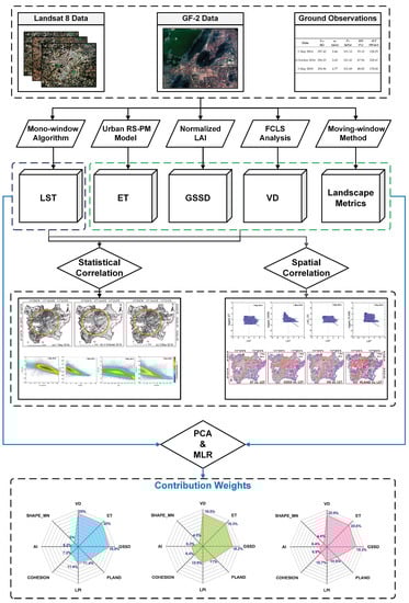
Figure 1.
Technical logic of this study.
2. Materials and Methods
2.1. Study Area
Situated in the northwest region of Jiangsu, China (Figure 2), Xuzhou serves as the central city of the Huaihai Economic Zone in China. Between 1995 and 2019, Xuzhou underwent a period of rapid urbanization, witnessing an expansion of its built-up area from 59 km2 to 274 km2. By the end of 2022, Xuzhou’s urbanization rate reached 66.81%. Xuzhou, being a typical intermediate-sized city in China, has well-developed industries in transportation, energy, and manufacturing, resulting in a significant UHI effect. In addition, Xuzhou has favorable climatic resources, with short spring and autumn seasons and long summer and winter seasons, which are conducive to the cultivation of various crops. The city’s forest cover has increased to 31.5% (by the end of 2022), which has proven to be highly effective in mitigating the urban heat environment. Thus, Xuzhou city was chosen as the study area due to its good representativeness. This study area encompasses not only the built-up areas of Xuzhou city, comprising Quanshan, Tongshan, Jiuli, Yunlong, and Gulou districts, but also some suburban regions.
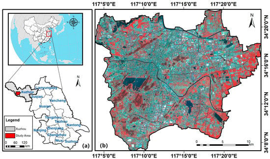
Figure 2.
(a) Geographical location of Xuzhou; (b) GF-2 image of the study area with false color band fusion.
2.2. Data Source and Preprocessing
Three Landsat 8 images were acquired from the data center of the United States Geological Survey (USGS) (https://glovis.usgs.gov/, accessed on 13 January 2023) for three periods from 2014 to 2018 (Table 1). The data were utilized to derive the LST and extract the urban green space cooling factors. Furthermore, a set of GaoFen-2 (GF-2) high-resolution remote sensing images were obtained to extract accurate land surface cover information for validating the mixed pixel decomposition. Meteorological data (Table 2), including air temperature (Tair), air relative humidity (RH), atmospheric pressure (PA), wind speed (uz), and latent heat flux observations (λET), which are necessary for land surface parameter calculations, were acquired from China University of Mining and Technology in the study area (Figure 3).

Table 1.
Technical information of Landsat 8 and GF-2 data.
Table 2.
Meteorological and latent heat flux data.
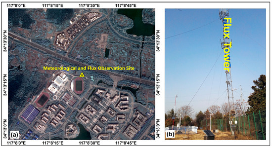
Figure 3.
(a) Location of the meteorological and flux observation site; (b) an eddy covariance (EC) system installed at 15 m height of the flux tower.
2.3. LST Retrieval
The USGS suggests utilizing the single-channel method that relies on the thermal infrared band 10 of Landsat 8 to retrieve the LST [23]. The improved mono-window algorithm [28] is an LST inversion method developed specifically for Landsat 8 data, which uses only two additional meteorological parameters, the near-surface air temperature (Tair) and the atmospheric transmittance (τ), to calculate the true LST [29]. The equations are as follows:
where a = −62.7182 and b = 0.4339 are the coefficients of the Planck blackbody radiation function for Landsat 8 band 10 in the range of 0 to 70 °C; T10 is the brightness temperature calculated from band 10 by Equation (4); ε is the land surface specific emissivity, which can be calculated by Equation (5); the regression relationship between τ and atmospheric water content (w) in summer at mid-latitudes was simulated and shown in Table 3 [30]; and w can be calculated from ground-based observed water vapor pressure data [31].
where K1 = 774.89 and K2 = 1321.08 are the preset constants of Landsat Band 10, respectively, available in the header file of the image; L10 is the radiometric brightness value transformed from the initial DN value of Band 10; Pv is the vegetation cover ratio, which can be calculated by NDVI; Rv is the radiance ratio of vegetation pixel; Rx is the radiance ratio of soil (Rs) or impervious surface pixel (Rimp) [30]; εv = 0.973 is the emissivity of pure vegetation pixel; εx is the emissivity of pure soil (εs = 0.966) or impervious surface (εimp = 0.962) pixel; and dε is the interaction value of the emissivity of each component in a pixel [29].
Table 3.
Atmospheric transmittance functions under different atmospheric water content for mid-latitude summer.
2.4. Urban Green Space Shading Degree Extraction
The shading cooling capability of green space is primarily achieved through the direct blocking of solar radiation by the vegetation canopy leaves; therefore, the degree of shading directly depends on the leaf area of the vegetation canopy. The LAI is the total surface area of leaves per unit area of vegetation, and its value directly affects the shading effect of vegetation on the ground. Therefore, the urban green space shading degree (GSSD) can be expressed by the standardized LAI. Currently, most LAI spatial and temporal distributions are extracted from multi/hyper-spectral remote sensing images. Previous studies used the vegetation indices calculated from Landsat data, including the Ratio of Vegetation Index (RVI), the Perpendicular Vegetation Index (PVI), the Soil-adjusted Vegetation Index (SAVI), the Modified Soil-adjusted Vegetation Index (MSAVI), the Atmospherically Resistant Vegetation Index (ARVI), and the Soil Atmospherically Resistant Vegetation Index (SARVI), which were regressed against the field-measured LAI. A multiple linear regression (MLR) model was ultimately identified as the best fit for the correlation between LAI and these indices [10,20], and the regression coefficient r and the fitting goodness R2 of this model were reported as 0.930 and 0.864 (p < 0.001), respectively. The equations are given below:
where NIR is the near infrared band; R is the red band; B is the blue band; L is the soil impact factor; and γ is the radiation correction coefficient of the optical path.
2.5. Vegetation Density Extraction
Vegetation density (VD) is the number or coverage ratio of plants per unit area and is an important factor affecting regional temperature regulation. The VD index in remote sensing images can be expressed by the vegetation ratio in each pixel through mixed pixel decomposition. According to the field survey, the endmembers, except for water, have been grouped into categories, including soil, forest, grassland, and impervious surfaces with high and low albedo. The vegetation endmembers (forest and grassland) in the urban mixed pixels were extracted using linear mixed spectral analysis (LMSA). The fully constrained linear mixture spectral analysis (FCLS), derived from LMSA, imposes the constraint that the total sum of component abundances must equal 100% [32]. The formula is as follows:
where fi is the abundance of component i; N = 5 is the number of component types; is the normalized reflectance of component i for band b; is the actual normalized reflectance; and eb is the error. After extracting the abundances of all endmembers, the vegetation fraction (i.e., VD) can be obtained by combining the forest abundance with grassland abundance.
To ensure the precision of VD, validation using high-resolution images is essential. A random scattering method was used to generate 100 random points on the study area image for 4 October 2016, and 100 sample areas (3 × 3 pixels of the component abundance image) were generated, centered on the pixels where these random points were located. All sample areas were overlaid with the GF-2 image (refer to Table 1), and the true vegetation proportions in the sample areas were extracted using a manual interpretation method and compared with the vegetation abundances in the corresponding areas. Finally, the extraction accuracy of VD was determined based on the linear regression of the true value and the Landsat 8 extracted value.
2.6. ET Estimation
ET includes both vegetation transpiration and soil water evaporation. Remote sensing technology provides an effective way to extract regional evapotranspiration. According to the assumption of the multi-source parallel model, vegetation and soil can be considered as two parallel parts, and the heat exchange between them can be ignored [33]. The remote sensing Penman–Menteith (RS-PM) model is widely used in ET estimation based on low- and medium-resolution remote sensing images because it requires relatively few meteorological parameters. The conventional RS-PM model assumes that only vegetation and soil components are mixed in a pixel. Therefore, vegetation transpiration (ETv) and soil water evaporation (ETs) can be calculated separately based on the FVC index [34,35]. However, mixed pixels in urban medium- and low-resolution satellite images typically comprise impervious surfaces, vegetation, soil, and other components, resulting in more complex endmember extraction and net radiation flux assignment in the pixel. Therefore, to estimate urban surface ET, the urban RS-PM model was developed [22], which is based on FCLS to extract the component abundance in an urban pixel, and the latent heat inversion parameterization scheme was improved, especially for urban surface characteristics. The algorithms are as follows:
where λ is the latent heat of water vaporization; fv and fs are the abundances of vegetation and soil components output through FCLS, respectively; △ is the curve slope of saturation water pressure (es); and are the net radiations of pure vegetation and soil pixels, respectively; is the heat flux of pure soil pixel; ρ is the air density; Cp is the specific heat capacity of air; ea is the actual water vapor pressure; rah,v and rah,s are the aerodynamic resistance of vegetation and soil, respectively; γ is the psychrometric constant; rs,v is the surface resistance of vegetation canopy transpiration; rtot is the sum of the surface resistance of soil water evaporation and aerodynamic resistance; and RH is the relative humidity of air.
2.6.1. Net Radiation Calculation
According to the natural or agricultural surface net radiation algorithm [34,36], the urban RS-PM model [22] improves the method of calculating the intermediate parameters of net radiation for each component based on urban surface characteristics. The equations used were as follows:
where av and as are the pure vegetation and soil albedos calculated by the Landsat 8 wide-band albedo algorithm [37]; Sd is the incident solar radiation, which can be calculated using the solar constant Isc (1367 W/m−2), the solar-terrestrial revision factor dm2, the solar zenith angle θ, the latitude φ, the solar declination δ, the solar time angle ω, and the wide-band atmospheric transmissivity τb [22,38]; εair is the atmospheric emissivity [39]; εv and εs are the pure vegetation and soil emissivity; Tair is the atmospheric temperature; and Tv and Ts are the component temperatures of vegetation and soil endmembers which can be estimated using the radiation ratio [30].
2.6.2. Aerodynamic Resistance Calculation
The aerodynamic resistance of vegetation (rah,v) and soil (rah,s) in the mixed pixel can be calculated using the following Equations [40]:
where Z is the height above ground for wind speed and air temperature observations; k = 0.41, which is the von Karman constant; uz is the observed wind speed at height Z; do,v, Zom,v, and Zoh,v are the zero-plane displacement, aerodynamic roughness length, and thermodynamic roughness length for the vegetation component, respectively, which can be estimated using Brutsaert et al. [41] and Kustas et al. [42]; and do,s, Zoh,s, and Zoh,s are the zero-plane displacement, aerodynamic roughness length, and thermodynamic roughness length for the soil component, respectively, and can be estimated using the methods proposed by Liu et al. [43] and Brutsaert et al. [41].
2.6.3. Surface Resistance Calculation
The vegetation component surface resistance (rs,v) can be calculated using the vegetation canopy water vapor conductivity gc, as shown in Equations (24)–(26):
where CL = 0.0013 is the empirical value of the mean potential stomatal water vapor conductivity per unit LAI [44]; m(Tmin) and m(VPD) represent air temperature and water vapor pressure stress functions calculated by the equation and look-up table [34].
The soil component surface resistance can be obtained by correcting the total surface aerodynamic impedance for the air temperature (Tair) and air pressure (PA) under standard conditions [34]:
2.6.4. Soil Heat Flux Calculation
Based on station observations, the soil heat was derived by soil component net radiation flux and solar zenith angle θ from station observations [19], as shown in Equation (29).
2.6.5. ET Validation
The footprint model considers the contribution of turbulence around an eddy covariance (EC) system, which can model the contributing source region corresponding to the EC observations in the ET inversion image and assign a normalized weight value to each pixel in the source region. This resulted in a weighted average of the ET inversion results for the source region that spatially matched the EC observations. The footprint models the problem of spatially matching ground flux observations with remote sensing inversion values, as shown in Equations (30) and (31) [45].
where x is the upwind distance; zm is the instrument observation height; Dy(x, y) is the lateral wind diffusion function; fy(x, zm) is the integrated lateral wind footprint function; λETi is the ET inversion value of pixel i in the source area; xi is the contribution weight of pixel i; and λETF is the ET remote sensing weighted inversion value of the source area.
2.7. Urban Green Space Landscape Patterns Extraction
2.7.1. Effective Urban Green Space Definition
In addition to large urban forests and grasslands, urban green space also includes scattered greenery alongside buildings and roads. Although these green spaces can be extracted through land cover classification, some pixels classified as vegetation still have a mixture of impervious surfaces. The effectiveness of vegetated pixels in mitigating the thermal environment depends on their vegetation abundance. Previous studies have demonstrated that the thermal environment can be effectively regulated only when the density of vegetation in the mixed pixels is above the medium level [46], which can be defined as effective green space. Therefore, the vegetation abundance fv extracted by the FCLS was classified into five levels by using the mean standard deviation (Table 4). Finally, patches with high and sub-high vegetation abundance were extracted as the effective green space of the study area.
Table 4.
Classification rules of vegetation abundance level.
2.7.2. Landscape Pattern of Effective Urban Green Space
Numerous investigations have demonstrated that vegetation spatial characteristics are important factors influencing environmental temperature; in particular, the area, shape, aggregation, and connectivity of vegetation patches have negative impacts on LST [26,27,46]. Landscape pattern as a geospatial index can quantify the spatial characteristics of EGS patches well. Based on previous studies [44], here, five class-level landscape metrics of percentage of landscape (PLAND), largest patch index (LPI), aggregation index (AI), mean patch shape index (SHAPE_MN), and patch cohesion index (COHESION) are used to represent the area proportion, predominance, aggregation, shape complexity, and natural connectivity of effective urban green space patches, respectively, and these metrics will represent the values of spatial cooling factors of green space. The equations are as follows:
where aij is the area of patch ij; A is the total landscape area; gii is the number of adjacent patches of the same landscape type i; pij is the perimeter (m) of patch ij; n is the total number of patches of landscape type i; and Z is the total number of cells in the landscape. The five class-level landscape metrics are calculated in Fragstats 4.2 by selecting the moving window method. This method uses a fixed-size window to assign the landscape index in its spatial extent to the center pixel of the window and moves it to the next position to continue the calculation. In this way, both the value of the landscape metrics and the spatial distribution can be obtained. According to Zhang et al. [46], the best grain size and spatial extent were set as 60 m and 780 m in moving window analysis, respectively. It should be noted that in order to spatially match the results of the landscape metrics calculated from the moving window, the resolutions of the LST and all other green space factor images were resampled to 60 m.
2.8. Bivariate Spatial Autocorrelation Model
Moran’s I, as a statistical measure for geographic elements, can characterize their spatial distribution and degree of correlation [47]. Bivariate global and local autocorrelation [48] established using Moran’s I index were employed to depict the correlation level between various factors’ spatial distribution, uncovering the association between spatial variables and other variables in adjacent areas. Bivariate global spatial autocorrelation analysis is utilized to investigate the spatial response of LST concerning each green space index, and the calculation equations are as follows:
where I represents the bivariate global spatial autocorrelation index that measures the overall correlation between the spatial distribution of independent variable x and dependent variable y; n denotes the total number of spatial cells; Mij represents the spatial weight matrix constructed using the K adjacency method; and xi and yj refer to the observed values of independent and dependent variables in spatial cells i and j, respectively. S2 signifies the variance of all samples.
To examine the spatial correlation of variable distribution within a local area, bivariate local spatial autocorrelation analysis was conducted. The local indicators of spatial association (LISA) distribution map, which is generated based on the z-test, can demonstrate the clustering and divergence traits of variables within a local area. The equations used for the calculation are as follows:
where is the local spatial relationship between the independent variable and the dependent variable of spatial cell i. is the value of attribute a located in spatial cell i; is the value of attribute b located in spatial cell j; and are the mean values of attributes a and b, respectively; and δa and δb are the variances of attributes a and b, respectively.
2.9. Principal Component Analysis
Standardized coefficients in MLR are frequently utilized to indicate the impact weight of multiple independent variables on dependent variables. Nevertheless, this method is unable to be directly applied when there is a correlation among the variables involved. By performing the orthogonal transformation, Principal Component Analysis (PCA) [49,50,51] converts a group of potentially correlated variables into a group of linearly uncorrelated principal component variables.
To eliminate the multicollinearity effect among all green space factors (Cj), the principal component variable Fi was converted [52], and then the standardized regression coefficients (βi) were calculated through MLR between LST and Fi, thus eliminating multicollinearity among the green space factors. Finally, the eigenvalues of the principal components (ηi), the initial variable influence coefficients of the principal components , and βi were employed to establish the contribution weight (Wj) of each green space factor to LST, which were shown as the following equations:
3. Results
3.1. LST Retrieval Results
Figure 4 illustrates the remote sensing inversion results of the LST during three phases, with average surface temperatures of 305 K, 309 K, and 305 K, respectively. The LST spatial distribution patterns during these three periods highlight that regions with higher LST are primarily concentrated in impervious surfaces, including commercial, industrial, and residential areas. Conversely, regions with lower LST are mainly present in vegetation-covered regions, including urban forests, grasslands, green belts, and suburban farmlands. This distribution indicates the potential alleviation impact of green space on the UHI.
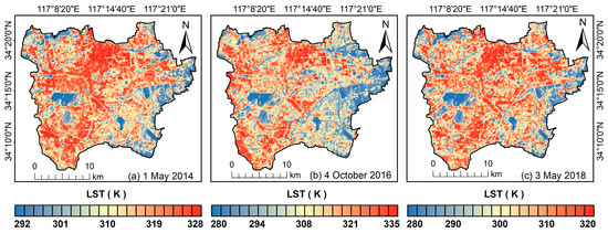
Figure 4.
LST retrieval results for three phases.
3.2. Green Space Factors Extraction Results
Figure 5 displays the spatial distribution of GSSD, ET, and VD, extracted from remote sensing data for 1 May 2014, 4 October 2016, and 3 May 2018. Owing to the complexity of the calculation process of ET and the subjectivity of the endmember selection process in the calculation of VD, it is necessary to validate the results of these two indices using flux observations and high-resolution satellite images, respectively. For the ET results, the validation results between the weighted inversion ET values of the source area and the flux observations in three periods are listed in Table 5, and the error rates of the three are −9.67%, 26.49%, and 21.03%, respectively.
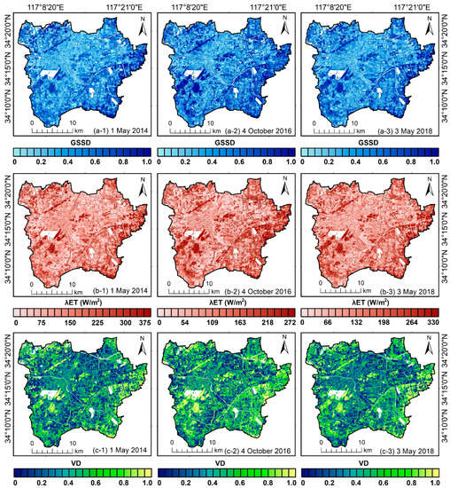
Figure 5.
The spatial distribution maps of (a-1–a-3) GSSD, (b-1–b-3) ET, and (c-1–c-3) VD on 1 May 2014, 4 October 2016, and 3 May 2018.
Table 5.
ET validation results.
Because high-resolution images for a date close to 4 October 2016 could not be acquired, only the VD remote sensing extraction result of 5 October 2016 was verified. However, considering that the extraction methods and endmember selection principles of VD are kept the same, the difference in VD remote sensing extraction accuracy between the three phases can be regarded as insignificant. Figure 6 presents the results of the accuracy validation for VD, revealing an R2 value of 0.866 (0.833 for soil endmember) between the remote sensing extracted values of VD and the actual values. These findings suggest that the precision of both ET and VD results was satisfactory, enabling their utilization for further analysis.
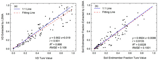
Figure 6.
Validation results of VD on 4 October 2016: (a) accuracy of VD extraction and (b) accuracy of soil endmember extraction.
3.3. Statistical Correlation Analysis
The standard deviational ellipse (SDE) indicates the primary direction and dispersion of geographic element distribution [53]. The LSTs of three phases were also divided into five UHI levels through the mean standard deviation method (Table 4), with low and sub-low LST patches designated as cool islands. SDEs were then calculated for effective green space (SDEg) and cool islands (SDEc), respectively. Figure 7 shows that the SDEg and SDEc of each period had a high degree of coincidence. Additionally, the mean centers of effective green space and cool islands for each phase were very close, with distances of 370.8 m, 1006.5 m, and 498.1 m, respectively. These results suggest a similar spatial distribution between effective green space and cool islands, supporting the preliminary evidence of the alleviation impact of green space on the UHI.
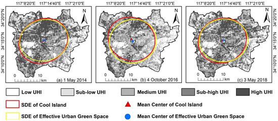
Figure 7.
The SDEs of the effective green space and cool island for three phases.
The images of LST and eight green space factors were superimposed, and scatter density maps were output (Figure 8). The density aggregation areas of the scatter cloud all showed a decreasing trend in the dependent variable (LST) with an increase in the independent variable (green space factors). The linear regression results further showed (Table 6) that all factors were significantly negatively linearly correlated with LST (p < 0.001), indicating that these factors played a role in reducing LST. Except for the SHAPE_MN, which has a moderate correlation [54] with LST (0.3 < |r| < 0.5), the other factors ET, GSSD, VD, PLAND, COHESION, LPI, and AI showed a strong correlation [54] with LST (|r| > 0.5). This indicates that the eight selected greenspace factors are effective cooling factors in mitigating the urban thermal environment. There were some variations in the ranking of the correlation coefficient values for each index among the three periods. For example, the green space index with the strongest correlation with LST on 4 October 2016 was VD, while on 1 May 2014 and 23 May 2018, it was GSSD. Therefore, it is not possible to directly determine the ranking of all green space cooling factors in terms of their influence on the thermal environment using correlation coefficients.
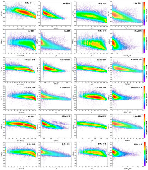
Figure 8.
Scatter density diagrams of LST versus the green space factors of ET, GSSD, PLAND, COHESION, AI, and SHAPE_MN of three phases.
Table 6.
Linear regression results of the green space factors with LST.
3.4. Spatial Correlation Analysis
Bivariate global spatial autocorrelation between LST and eight green space factors in three periods were calculated using OpenGeoda software (Table 7), and the results showed that all green space factors showed a significant negative spatial correlation with the LST (Moran’s I < 0, p < 0.001), that is, the increase in green space factors in the local area leads to the decrease in LST in the surrounding area. Except for the SHAPE_MN, which showed a moderate spatial correlation with LST (0.3 < |Moran’s I| < 0.5), the other factors all showed a strong spatial correlation with LST (|Moran’s I| > 0.5). The strongest correlation with LST on 4 October 2016 was PLAND, while on 1 May 2014 and 3 May 2018, it was GSSD.
Table 7.
Global Moran’s I of the green space factors with LST.
Further analyses of the bivariate local spatial autocorrelation of the LST with the green space factors for three periods are shown in Figure 9 and Figure 10. Moran’s scatter plot (Figure 9) shows that most scatter clouds are concentrated in the second and fourth quadrants, and the spatial clustering mode of LST and green space factors in LISA maps (Figure 10) is dominated by HL and LH. The above phenomenon indicated that pixels with higher (or lower) greenspace factors clustered around pixels with lower (or higher) LST. This provides further evidence for the spatial impact of greenspace factors in mitigating UHIs. However, the ranking of Moran’s I values remained highly variable among the three periods; thus, the weight of the effect of greenspace factors on LST could also not be revealed directly through spatial correlation.
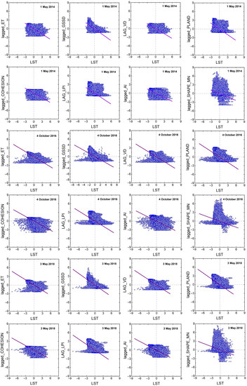
Figure 9.
Moran scatter plot of LST versus the green space factors of ET, GSSD, PLAND, COHESION, AI, and SHAPE_MN for three periods.
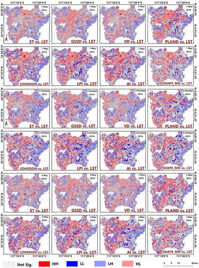
Figure 10.
LISA maps of LST with green space factors (HH represents high LST spatially aggregated with high green space index; LL represent low LST spatially aggregated with low green space index; HL refers to high LST spatially aggregated with low green space index; and LH refers to low LST spatially aggregated with high green space index).
3.5. Contribution Weights of Urban Green Space Factors on LST
Statistical correlation and spatial correlation analyses can demonstrate the impact direction and degree of each green space factor on LST, respectively. However, this single-variable analysis cannot directly reflect the contribution weight of each greenspace index in mitigating environmental temperature under the effect of multiple factors. MLR can model the LST as a function of all greenspace factors, and the standardized regression coefficient of each index can represent the corresponding impact weight. However, some of the selected green space factors were calculated using the same remote sensing image bands, or the same intermediate parameters were used in the calculation, which led to the discovery of multiple covariances among some variables in the test (variance inflation factor, VIF > 5), resulting in an inability to use MLR directly.
Therefore, PCA was applied to all initial variables to extract the principal component variables (initial LST and green space factors were normalized) to eliminate correlations between initial variables. Table 8 indicates that the Kaiser–Meyer–Olkin measure of sampling adequacy (KMO) values for the three periods are 0.796, 0.808, and 0.788, respectively. These values demonstrate that the PCA can be applied to the eight independent variables. Two principal components (F1 and F2) were extracted from each period of the independent variables, and their cumulative proportions of variance are 82.04%, 82.99%, and 84.37%, respectively, demonstrating their effectiveness in representing all independent variables.
Table 8.
KMO and Bartlett’s test and total variance explained.
Table 9 describes the influence coefficients (θ1j and θ2j) of all standardized initial independent variables (C1 to C8) in principal component variables (F1 and F2). The ranking of the θij values of the two principal components showed that F1 reflected the influence of vegetation factors on LST, and F2 reflected the influence of spatial pattern metrics on LST.
Table 9.
Influence coefficients matrix of the green space factors in principal components F1 and F2.
The results of the MLR with F1 and F2 as the independent variables and normalized LST as the dependent variable are listed in Table 10. There was a strong correlation (r > 0.71) and a significant and strong negative linear correlation (R2 > 0.50, p < 0.001) between the principal component independent variables and the dependent variable in three periods. Standardized regression coefficients β1 and β2 were used as the impact weights of F1 and F2, respectively, on LST. Finally, the contribution weight Wj of each green space factor on LST was calculated using Equation (43) by combining the influence coefficients of C1 to C8 on F1 and F2. The results are presented in Figure 11.
Table 10.
MLR coefficients between normalized LST and F1 and F2.
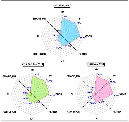
Figure 11.
The radar chart of the contribution weight of eight green space factors on LST.
The Wj for the three periods in descending order are VD ≥ ET > GSSD > PLAND ≈ LPI > COHESION > AI > SHAPE_MN, and the vegetation factors of urban green space (VD, ET, and GSSD) contribute more to UHI mitigation than its spatial pattern factors (PLAND, LPI, COHESION, AI, and SHAPE_MN). In addition, the weight values differed slightly (0.1% to 0.5%) between VD and ET, PLAND and LPI, and COHESION and AI, indicating that each pair of factors had a similar contribution to mitigating the thermal environment.
4. Discussion
Numerous vegetation indices and spatial characteristics metrics of urban green space have been demonstrated to have regulatory effects on the UHI. Concerning the association between vegetation indices and LST, a prior investigation indicated that NDVI is negatively linearly correlated with LST [55]. Moreover, it has been demonstrated that the FVC index exhibits a robust negative correlation with LST (r = −0.734) [51]. As FVC increased, the reduction in LST was more prominent, especially when FVC exceeded 0.2; for every 10% rise in FVC, the LST dropped by approximately 1.1 °C [56]. This is in line with our findings that LST is significantly negatively correlated with VD. Unlike FVC, which is obtained by band math of multispectral images, the VD index is extracted through FCLS. However, both VD and FVC represent the vegetation area ratio (or vegetation coverage density) in a single pixel, so their impact on the LST is close. There are limited techniques available for extracting the vegetation canopy shading index directly from remote sensing images with low to medium resolution. Considering that the shading function of vegetation per unit area mainly depends on the vegetation leaf area, the normalized LAI index [10,20] was utilized in our study to represent the shading degree index (GSSD) of green space. This method cannot accurately calculate the shading area of the vegetation. However, it can approximately simulate the shading intensity of the vegetation leaves within each pixel. Our findings demonstrate that LST is significantly negatively correlated with GSSD both quantitatively and spatially, which is consistent with a prior report suggesting that LAI is significantly correlated with the cooling intensity (r = 0.58) [10]. ET is a direct indicator of energy transformation resulting from the water–heat exchange between vegetation and the environment. Previous studies have also found that the influence of ET on UHIs becomes relatively weak during the cold season (November to April), while it has a more significant effect during the warm season (May to October) [23]. As the dates used in our study fall under the warm season (May to October), the results demonstrate a strong negative linear as well as spatial correlation between ET and LST.
Studies investigating the influence of green space spatial distribution on LST usually employ the grid-based approach to divide the study area into cells, followed by calculating landscape metrics and average LST for each grid unit separately [57]. This approach can obtain spatial distribution maps of landscape metrics but with low spatial resolution (generally between 200 m × 200 m and 5000 m × 5000 m) [24,26]. The spatial resolution of the landscape metric map output by the moving window method used in this study was consistent with the selected grain size (60 m × 60 m), which was closer to the spatial resolution of the LST inversion image. This not only makes the landscape index distribution characteristics more detailed but also enables us to obtain more samples, which is beneficial for analyzing the quantitative and spatial correlations between LST and green space landscape metrics. Prior investigations have compared the correlation of LST with various landscape metrics of greenspace patches [27]; the results showed that the correlation with PLAND is the highest. Additionally, the correlation coefficient of AI was higher than that of SHAPE_MN [26]. Other studies analyzed the linear relationships between LST and LPI, AI, and SHAPE_MN of green space patches and found that LPI had the highest goodness of fit (R2 = 0.41, p < 0.001), whereas SHAPE_MN had the lowest (R2 = 0.12, p < 0.001) [24]. Our results are consistent with these findings as well.
Our study used PCA to extract two principal component variables from the eight factors (initial variables) [52]. The standardized coefficients were obtained using MLR of the principal component variables with LST, which were multiplied by the impact weights of the initial variables in the principal components to obtain the contribution weights of the eight urban greenspace factors in mitigating the thermal environment. This method of weight calculation has two advantages. First, it can avoid the fact that the direct MLR of eight green space factors with LST appears to have positive normalized coefficients for some factors, which is the opposite of the actual situation. The second is to eliminate multicollinearity among the eight factors, which makes the results of the contribution weights more reasonable. The contribution weights of the eight factors indicate that increasing vegetation density is the preferred way to mitigate the UHI effect. Second, increasing broad-leaved forests with high ET and shading levels in urban greenery is also an effective way to reduce ambient temperature. In addition, enhancing the connectivity or aggregation between green space patches can enhance their cooling capacity. Because the green space shape characteristics contribute the least to the regulation of LST, they can be the lowest priority factor in urban green space planning.
5. Conclusions
Based on the Landsat 8 data, three vegetation indices and five landscape pattern metrics of urban green space were extracted as cooling factors. Statistical analysis and bivariate spatial autocorrelation analysis were applied to demonstrate the linear negative correlation and negative spatial correlation between these eight indicators and LST. PCA and MLR were applied to derive the contribution weights of the eight indicators for mitigating the UHI. The results indicate green space vegetation indices contribute more weight to the reduction in urban ambient temperature than the spatial pattern metrics. VD was the most effective cooling factor, followed by ET and GSSD. For the green space spatial patterns, PLAND and LPI make the major contribution in UHI mitigation, followed by COHESION and AI, and SHAPE_MN had the least contribution in reducing the ambient temperature. The results revealed differences in the characteristic factors of urban green space in mitigating UHI, which serve as a valuable reference in urban planning and climate enhancement.
This paper solely examined the cooling factors affecting the urban thermal environment, without taking into account other factors that influence urban temperatures, particularly those that contribute to warming. In future studies, it would be beneficial to comprehensively consider both cooling and warming factors in order to more reasonably model the contribution of various factors to changes in urban thermal conditions.
Author Contributions
Conceptualization, Y.Z. and Y.W.; methodology, Y.W.; software, N.D.; validation, Y.W.; formal analysis, Y.W.; data curation, Y.Z.; writing—original draft preparation, Y.Z.; writing—review and editing, Y.Z.; visualization, N.D. and X.Y.; supervision, X.Y.; funding acquisition, Y.W. and Y.Z. All authors have read and agreed to the published version of the manuscript.
Funding
This research was funded by the National Natural Science Foundation of China, Grant Nos. 42101049 and 42101256, and A Project Funded by the Priority Academic Program Development of Jiangsu Higher Education Institutions (PAPD).
Data Availability Statement
Not applicable.
Acknowledgments
The authors would like to thank the editor and the anonymous reviewers for their valuable comments and suggestions.
Conflicts of Interest
The authors declare no conflict of interest.
References
- Oke, T.R. The Energetic Basis of the Urban Heat Island. Q. J. R. Meteorol. Soc. 1982, 108, 1–24. [Google Scholar] [CrossRef]
- Tran, H.; Uchihama, D.; Ochi, S.; Yasuoka, Y. Assessment with Satellite Data of the Urban Heat Island Effects in Asian Mega Cities. Int. J. Appl. Earth Obs. Geoinf. 2006, 8, 34–48. [Google Scholar] [CrossRef]
- Kandel, H.; Melesse, A.; Whitman, D. An Analysis on the Urban Heat Island Effect Using Radiosonde Profiles and Landsat Imagery with Ground Meteorological Data in South Florida. Int. J. Remote Sens. 2016, 37, 2313–2337. [Google Scholar] [CrossRef]
- Sobrino, J.A.; Irakulis, I. A Methodology for Comparing the Surface Urban Heat Island in Selected Urban Agglomerations Around the World from Sentinel-3 SLSTR Data. Remote Sens. 2020, 12, 2052. [Google Scholar] [CrossRef]
- Estoque, R.C.; Murayama, Y. Monitoring Surface Urban Heat Island Formation in a Tropical Mountain City Using Landsat Data (1987–2015). ISPRS J. Photogramm. Remote Sens. 2017, 133, 18–29. [Google Scholar] [CrossRef]
- Zhang, Y.; Wang, Y.; Ding, N.; Yang, X. Spatial Pattern Impact of Impervious Surface Density on Urban Heat Island Effect: A Case Study in Xuzhou, China. Land 2022, 11, 2135. [Google Scholar] [CrossRef]
- Chen, X.; Wang, Z.; Bao, Y. Cool Island Effects of Urban Remnant Natural Mountains for Cooling Communities: A Case Study of Guiyang, China. Sustain. Cities Soc. 2021, 71, 102983. [Google Scholar] [CrossRef]
- Rakoto, P.Y.; Deilami, K.; Hurley, J.; Amati, M.; Sun, Q. (Chayn) Revisiting the Cooling Effects of Urban Greening: Planning Implications of Vegetation Types and Spatial Configuration. Urban For. Urban Green. 2021, 64, 127266. [Google Scholar] [CrossRef]
- Bartholy, J.; Pongrácz, R. A Brief Review of Health-Related Issues Occurring in Urban Areas Related to Global Warming of 1.5 °C. Curr. Opin. Environ. Sustain. 2018, 30, 123–132. [Google Scholar] [CrossRef]
- Sun, X.; Tan, X.; Chen, K.; Song, S.; Zhu, X.; Hou, D. Quantifying Landscape-Metrics Impacts on Urban Green-Spaces and Water-Bodies Cooling Effect: The Study of Nanjing, China. Urban For. Urban Green. 2020, 55, 126838. [Google Scholar] [CrossRef]
- Xiao, X.D.; Dong, L.; Yan, H.; Yang, N.; Xiong, Y. The Influence of the Spatial Characteristics of Urban Green Space on the Urban Heat Island Effect in Suzhou Industrial Park. Sustain. Cities Soc. 2018, 40, 428–439. [Google Scholar] [CrossRef]
- Zhang, Y.; Murray, A.T.; Turner, B.L. Optimizing Green Space Locations to Reduce Daytime and Nighttime Urban Heat Island Effects in Phoenix, Arizona. Landsc. Urban Plan. 2017, 165, 162–171. [Google Scholar] [CrossRef]
- Chang, C.-R.; Li, M.-H.; Chang, S.-D. A Preliminary Study on the Local Cool-Island Intensity of Taipei City Parks. Landsc. Urban Plan. 2007, 80, 386–395. [Google Scholar] [CrossRef]
- Masoudi, M.; Tan, P.Y.; Liew, S.C. Multi-City Comparison of the Relationships between Spatial Pattern and Cooling Effect of Urban Green Spaces in Four Major Asian Cities. Ecol. Indic. 2019, 98, 200–213. [Google Scholar] [CrossRef]
- Rahman, M.A.; Moser, A.; Rötzer, T.; Pauleit, S. Within Canopy Temperature Differences and Cooling Ability of Tilia Cordata Trees Grown in Urban Conditions. Build. Environ. 2017, 114, 118–128. [Google Scholar] [CrossRef]
- Yan, H.; Wu, F.; Dong, L. Influence of a Large Urban Park on the Local Urban Thermal Environment. Sci. Total Environ. 2018, 622–623, 882–891. [Google Scholar] [CrossRef]
- Chow, W.T.L.; Pope, R.L.; Martin, C.A.; Brazel, A.J. Observing and Modeling the Nocturnal Park Cool Island of an Arid City: Horizontal and Vertical Impacts. Theor. Appl. Climatol. 2011, 103, 197–211. [Google Scholar] [CrossRef]
- Spronken-Smith, R.A.; Oke, T.R. The Thermal Regime of Urban Parks in Two Cities with Different Summer Climates. Int. J. Remote Sens. 1998, 19, 2085–2104. [Google Scholar] [CrossRef]
- Bowler, D.E.; Buyung-Ali, L.; Knight, T.M.; Pullin, A.S. Urban Greening to Cool Towns and Cities: A Systematic Review of the Empirical Evidence. Landsc. Urban Plan. 2010, 97, 147–155. [Google Scholar] [CrossRef]
- Fei, Y.; Jiulin, S.; Hongliang, F.; Zuofang, Y.; Jiahua, Z.; Yunqiang, Z.; Kaishan, S.; Zongming, W.; Maogui, H. Comparison of Different Methods for Corn LAI Estimation over Northeastern China. Int. J. Appl. Earth Obs. Geoinf. 2012, 18, 462–471. [Google Scholar] [CrossRef]
- Weng, Q.; Rajasekar, U.; Hu, X. Modeling Urban Heat Islands and Their Relationship With Impervious Surface and Vegetation Abundance by Using ASTER Images. IEEE Trans. Geosci. Remote Sens. 2011, 49, 4080–4089. [Google Scholar] [CrossRef]
- Zhang, Y.; Li, L.; Qin, K.; Wang, Y.; Chen, L.; Yang, X. Remote Sensing Estimation of Urban Surface Evapotranspiration Based on a Modified Penman–Monteith Model. J. Appl. Remote Sens. 2018, 12, 046006. [Google Scholar] [CrossRef]
- Wang, Y.; Zhang, Y.; Ding, N.; Qin, K.; Yang, X. Simulating the Impact of Urban Surface Evapotranspiration on the Urban Heat Island Effect Using the Modified RS-PM Model: A Case Study of Xuzhou, China. Remote Sens. 2020, 12, 578. [Google Scholar] [CrossRef]
- Hou, H.; Estoque, R.C. Detecting Cooling Effect of Landscape from Composition and Configuration: An Urban Heat Island Study on Hangzhou. Urban For. Urban Green. 2020, 53, 126719. [Google Scholar] [CrossRef]
- Zawadzka, J.E.; Harris, J.A.; Corstanje, R. A Simple Method for Determination of Fine Resolution Urban Form Patterns with Distinct Thermal Properties Using Class-Level Landscape Metrics. Landsc. Ecol. 2021, 36, 1863–1876. [Google Scholar] [CrossRef]
- Estoque, R.C.; Murayama, Y.; Myint, S.W. Effects of Landscape Composition and Pattern on Land Surface Temperature: An Urban Heat Island Study in the Megacities of Southeast Asia. Sci. Total Environ. 2017, 577, 349–359. [Google Scholar] [CrossRef] [PubMed]
- Yao, L.; Li, T.; Xu, M.; Xu, Y. How the Landscape Features of Urban Green Space Impact Seasonal Land Surface Temperatures at a City-Block-Scale: An Urban Heat Island Study in Beijing, China. Urban For. Urban Green. 2020, 52, 126704. [Google Scholar] [CrossRef]
- Wang, F.; Qin, Z.; Song, C.; Tu, L.; Karnieli, A.; Zhao, S. An Improved Mono-Window Algorithm for Land Surface Temperature Retrieval from Landsat 8 Thermal Infrared Sensor Data. Remote Sens. 2015, 7, 4268–4289. [Google Scholar] [CrossRef]
- Qin, Z.; Karnieli, A.; Berliner, P. A Mono-Window Algorithm for Retrieving Land Surface Temperature from Landsat TM Data and Its Application to the Israel-Egypt Border Region. Int. J. Remote Sens. 2001, 22, 3719–3746. [Google Scholar] [CrossRef]
- Mao, K.; Qin, Z.; Shi, J.; Gong, P. A Practical Split-Window Algorithm for Retrieving Land-Surface Temperature from MODIS Data. Int. J. Remote Sens. 2005, 26, 3181–3204. [Google Scholar] [CrossRef]
- Zhang, Y.; Li, L.; Chen, L.; Liao, Z.; Wang, Y.; Wang, B.; Yang, X. A Modified Multi-Source Parallel Model for Estimating Urban Surface Evapotranspiration Based on ASTER Thermal Infrared Data. Remote Sens. 2017, 9, 1029. [Google Scholar] [CrossRef]
- Wu, C. Normalized Spectral Mixture Analysis for Monitoring Urban Composition Using ETM+ Imagery. Remote Sens. Environ. 2004, 93, 480–492. [Google Scholar] [CrossRef]
- Norman, J.M.M.; Kustas, W.P.P.; Humes, K.S.S. Source Approach for Estimating Soil and Vegetation Energy Fluxes in Observations of Directional Radiometric Surface Temperature. Agric. For. Meteorol. 1995, 77, 263–293. [Google Scholar] [CrossRef]
- Mu, Q.; Heinsch, F.A.; Zhao, M.; Running, S.W. Development of a Global Evapotranspiration Algorithm Based on MODIS and Global Meteorology Data. Remote Sens. Environ. 2007, 111, 519–536. [Google Scholar] [CrossRef]
- Mu, Q.; Zhao, M.; Running, S.W. Improvements to a MODIS Global Terrestrial Evapotranspiration Algorithm. Remote Sens. Environ. 2011, 115, 1781–1800. [Google Scholar] [CrossRef]
- Cleugh, H.A.; Leuning, R.; Mu, Q.; Running, S.W. Regional Evaporation Estimates from Flux Tower and MODIS Satellite Data. Remote Sens. Environ. 2007, 106, 285–304. [Google Scholar] [CrossRef]
- Liang, S.; Shuey, C.J.; Russ, A.L.; Fang, H.; Chen, M.; Walthall, C.L.; Daughtry, C.S.T.; Hunt, R. Narrowband to Broadband Conversions of Land Surface Albedo: II. Validation. Remote Sens. Environ. 2003, 84, 25–41. [Google Scholar] [CrossRef]
- Spencer, J.W. Fourier Series Representation of the Position of the Sun. Search 1971, 2, 172. [Google Scholar]
- Brutsaert, W. On a Derivable Formula for Long-wave Radiation from Clear Skies. Water Resour. Res. 1975, 11, 742–744. [Google Scholar] [CrossRef]
- Kustas, W.P.; Norman, J.M. Evaluation of Soil and Vegetation Heat Flux Predictions Using a Simple Two-Source Model with Radiometric Temperatures for Partial Canopy Cover. Agric. For. Meteorol. 1999, 94, 13–29. [Google Scholar] [CrossRef]
- Brutsaert, W. Evaporation into the Atmosphere: Theory, History and Applications; Springer: Berlin, The Netherlands, 1982; ISBN 978-90-277-1247-9. [Google Scholar]
- Kustas, W.P.; Choudhury, B.J.; Moran, M.S.; Reginato, R.J.; Jackson, R.D.; Gay, L.W.; Weaver, H.L. Determination of Sensible Heat Flux over Sparse Canopy Using Thermal Infrared Data. Agric. For. Meteorol. 1989, 44, 197–216. [Google Scholar] [CrossRef]
- Liu, S.; Lu, L.; Mao, D.; Jia, L. Evaluating Parameterizations of Aerodynamic Resistance to Heat Transfer Using Field Measurements. Hydrol. Earth Syst. Sci. 2007, 11, 769–783. [Google Scholar] [CrossRef]
- Leuning, R.; Zhang, Y.Q.; Rajaud, A.; Cleugh, H.; Tu, K. A Simple Surface Conductance Model to Estimate Regional Evaporation Using MODIS Leaf Area Index and the Penman-Monteith Equation. Water Resour. Res. 2008, 44, W10419. [Google Scholar] [CrossRef]
- Jia, Z.; Liu, S.; Xu, Z.; Chen, Y.; Zhu, M. Validation of Remotely Sensed Evapotranspiration over the Hai River Basin, China. J. Geophys. Res. Atmos. 2012, 117, D13113. [Google Scholar] [CrossRef]
- Zhang, Y.; Wang, Y.; Ding, N. Spatial Effects of Landscape Patterns of Urban Patches with Different Vegetation Fractions on Urban Thermal Environment. Remote Sens. 2022, 14, 5684. [Google Scholar] [CrossRef]
- Zhang, Y.; Liu, Y.; Zhang, Y.; Liu, Y.; Zhang, G.; Chen, Y. On the Spatial Relationship between Ecosystem Services and Urbanization: A Case Study in Wuhan, China. Sci. Total Environ. 2018, 637–638, 780–790. [Google Scholar] [CrossRef]
- Anselin, L. Local Indicators of Spatial Association—LISA. Geogr. Anal. 1995, 27, 93–115. [Google Scholar] [CrossRef]
- Uddin, M.N.; Saiful Islam, A.K.M.; Bala, S.K.; Islam, G.M.T.; Adhikary, S.; Saha, D.; Haque, S.; Fahad, M.G.R.; Akter, R. Mapping of Climate Vulnerability of the Coastal Region of Bangladesh Using Principal Component Analysis. Appl. Geogr. 2019, 102, 47–57. [Google Scholar] [CrossRef]
- Wu, T. Quantifying Coastal Flood Vulnerability for Climate Adaptation Policy Using Principal Component Analysis. Ecol. Indic. 2021, 129, 108006. [Google Scholar] [CrossRef]
- Ren, Z.; Li, Z.; Wu, F.; Ma, H.; Xu, Z.; Jiang, W.; Wang, S.; Yang, J. Spatiotemporal Evolution of the Urban Thermal Environment Effect and Its Influencing Factors: A Case Study of Beijing, China. ISPRS Int. J. Geo-Inf. 2022, 11, 278. [Google Scholar] [CrossRef]
- Liu, R.X.; Kuang, J.; Gong, Q.; Hou, X.L. Principal Component Regression Analysis with Spss. Comput. Methods Programs Biomed. 2003, 71, 141–147. [Google Scholar] [CrossRef] [PubMed]
- Mamuse, A.; Porwal, A.; Kreuzer, O.; Beresford, S. A New Method for Spatial Centrographic Analysis of Mineral Deposit Clusters. Ore Geol. Rev. 2009, 36, 293–305. [Google Scholar] [CrossRef]
- Cohen, J. Statistical Power Analysis for the Behavioral Sciences, 2nd ed.; Lawrence Earlbaum Associates: Hillsdale, NY, USA, 1988; ISBN 0805802835. [Google Scholar]
- Zhang, Y.; Zhan, Y.; Yu, T.; Ren, X. Urban Green Effects on Land Surface Temperature Caused by Surface Characteristics: A Case Study of Summer Beijing Metropolitan Region. Infrared Phys. Technol. 2017, 86, 35–43. [Google Scholar] [CrossRef]
- Li, Y.; Wang, X.; Chen, Y.; Wang, M. Land Surface Temperature Variations and Their Relationship to Fractional Vegetation Coverage in Subtropical Regions: A Case Study in Fujian Province, China. Int. J. Remote Sens. 2020, 41, 2081–2097. [Google Scholar] [CrossRef]
- Elliot, T.; Babí Almenar, J.; Rugani, B. Modelling the Relationships between Urban Land Cover Change and Local Climate Regulation to Estimate Urban Heat Island Effect. Urban For. Urban Green. 2020, 50, 126650. [Google Scholar] [CrossRef]


Disclaimer/Publisher’s Note: The statements, opinions and data contained in all publications are solely those of the individual author(s) and contributor(s) and not of MDPI and/or the editor(s). MDPI and/or the editor(s) disclaim responsibility for any injury to people or property resulting from any ideas, methods, instructions or products referred to in the content. |
© 2023 by the authors. Licensee MDPI, Basel, Switzerland. This article is an open access article distributed under the terms and conditions of the Creative Commons Attribution (CC BY) license (https://creativecommons.org/licenses/by/4.0/).