


Confidence-Guided Planar-Recovering Multiview Stereo for Weakly Textured Plane of High-Resolution Image Scenes

Abstract
1. Introduction
- (1)
- Depending on the photometric consistency, traditional depth estimation [6,7] exhibits the fuzzy matching problem in weakly textured regions. The fuzzy matching problem is that even the erroneous plane hypothesis allows patches to match highly similar regions between multiple views. This makes depth estimation insufficiently reliable in weakly textured regions.
- (2)
- During depth estimation, some views are invisible and cannot accurately reflect a reliable matching relationship due to occlusion and illumination. The matching cost calculated via invisible view would be an outlier in the multiview matching cost, which affects the accuracy of depth estimation.
- To quantify the reliability of the plane hypothesis in depth estimation, a plane hypothesis confidence calculation is proposed. The confidence consists of multiview confidence and patch confidence, which provide global geometry information and local depth consistency.
- Based on the confidence calculation, a plane supplement module is applied to generate reliable plane hypotheses and is introduced into the confidence-driven depth estimation to tackle the estimating problem of weakly textured regions to achieve the high completeness of reconstruction.
- An adaptive depth fusion method is proposed to address the imbalance in accuracy and completeness of point clouds caused by fixed parameters. The view constraint and consistency constraints for fusion are adaptively adjusted according to the dependency of each view on different neighboring views. The method achieves a good balance of accuracy and completeness when merging depth maps into dense point clouds.
2. Related Works
3. Review of Depth Estimation in ACMH
3.1. Initialization
3.2. Propagation
3.3. Multiview Matching Cost Calculation
3.4. Refinement
4. Method
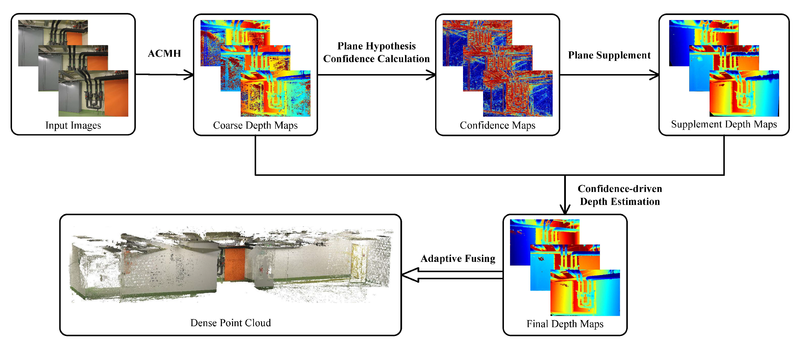
4.1. Overview
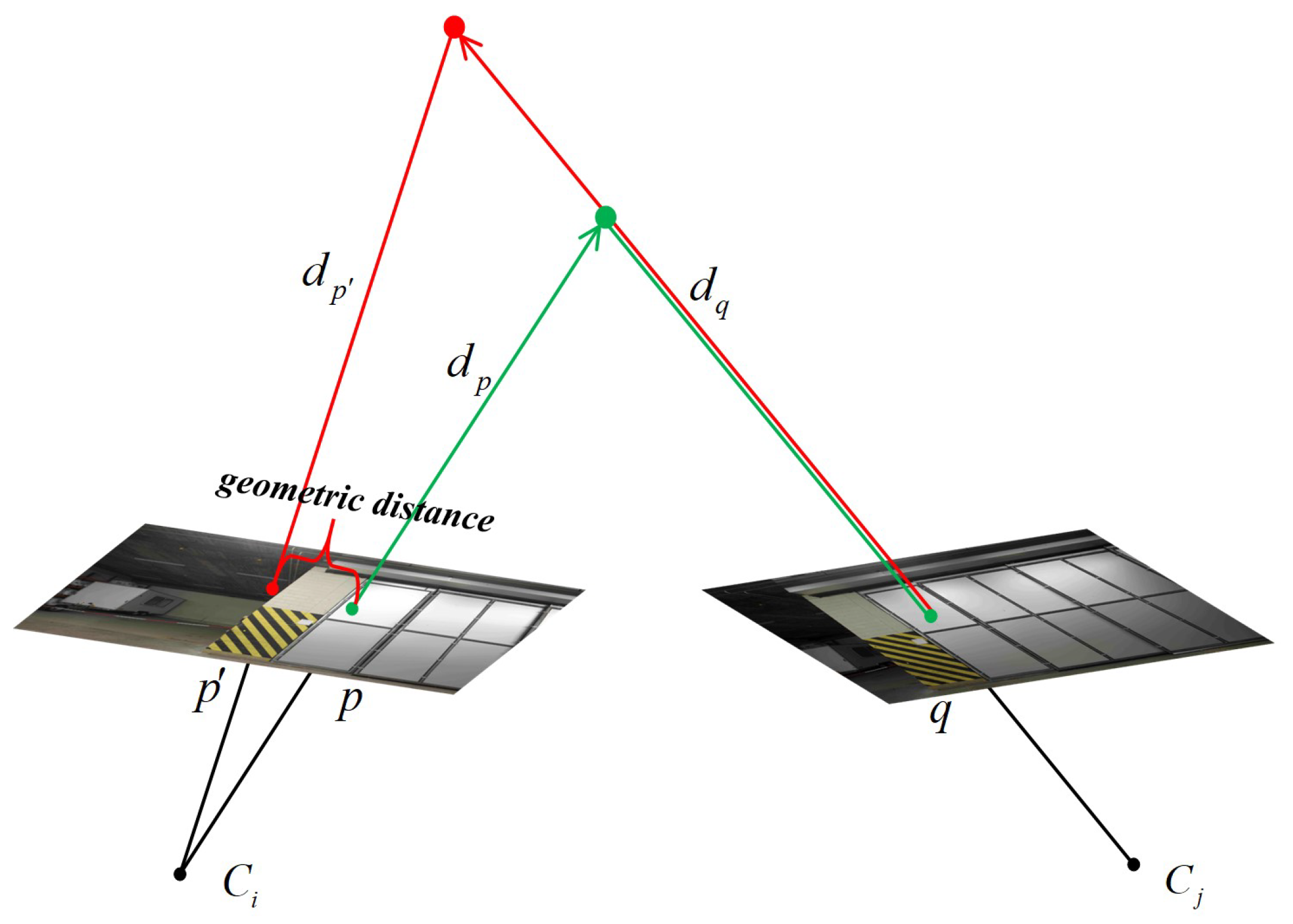
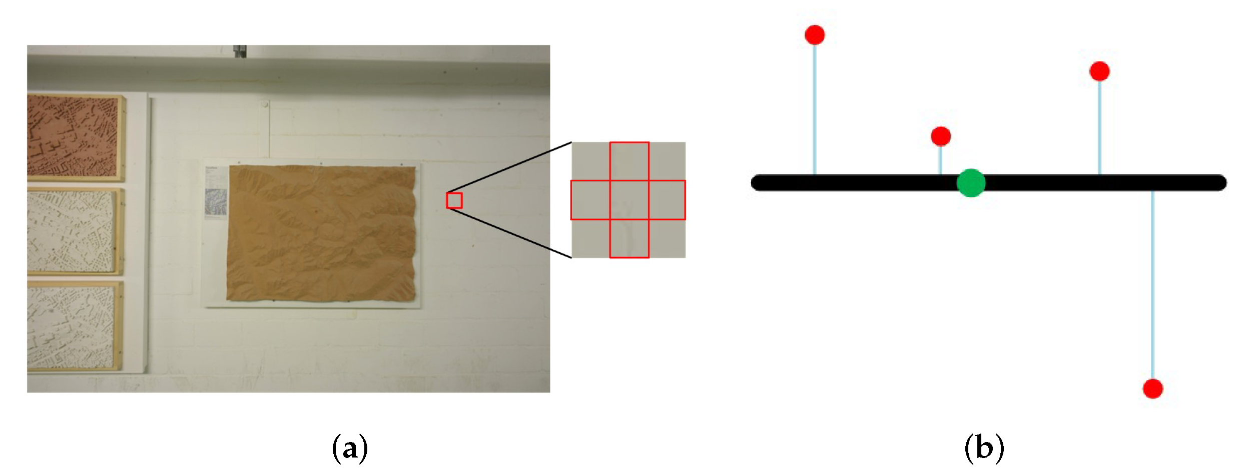
4.2. Plane Hypothesis Confidence Calculation
4.3. Plane Supplement and Confidence-Driven Depth Estimation
4.4. Adaptive Fusion
5. Experiments
5.1. Parameter Settings
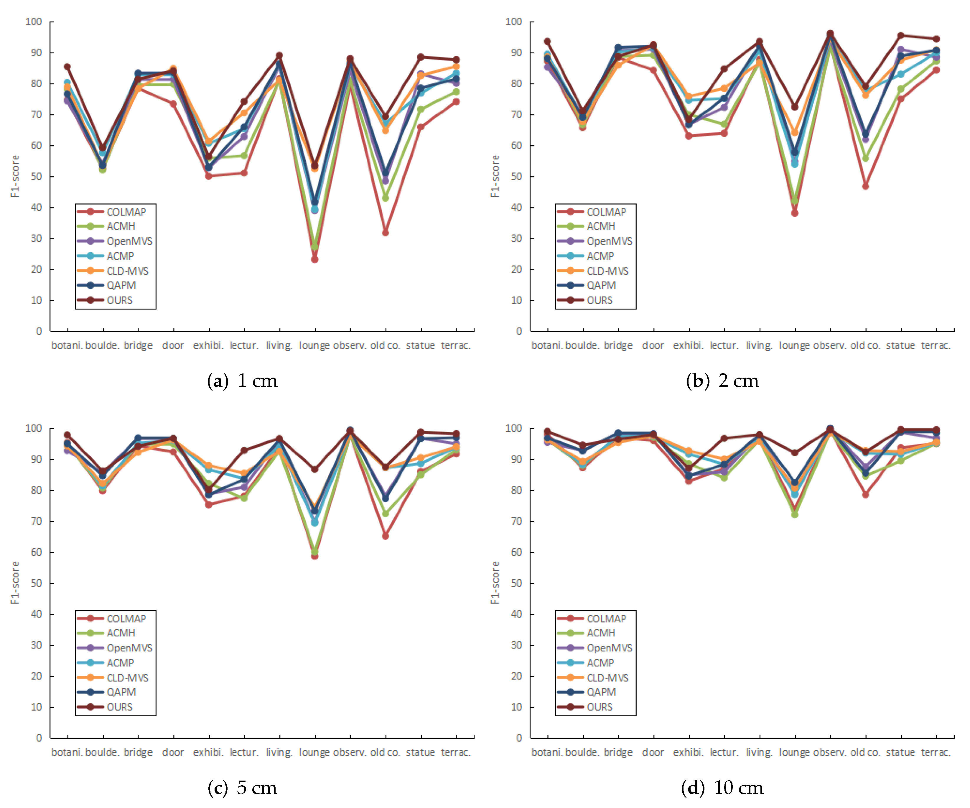
5.2. Quantification
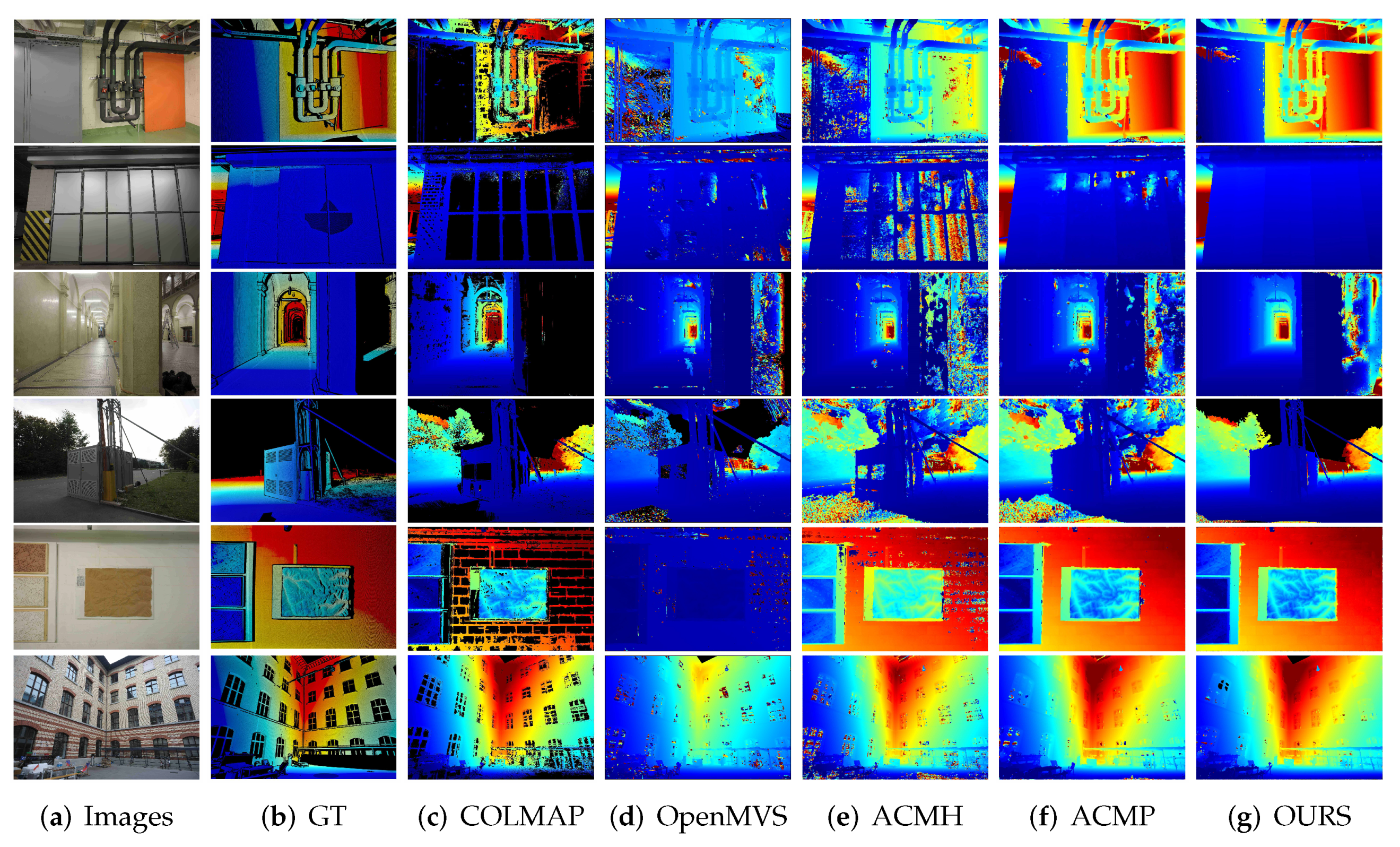
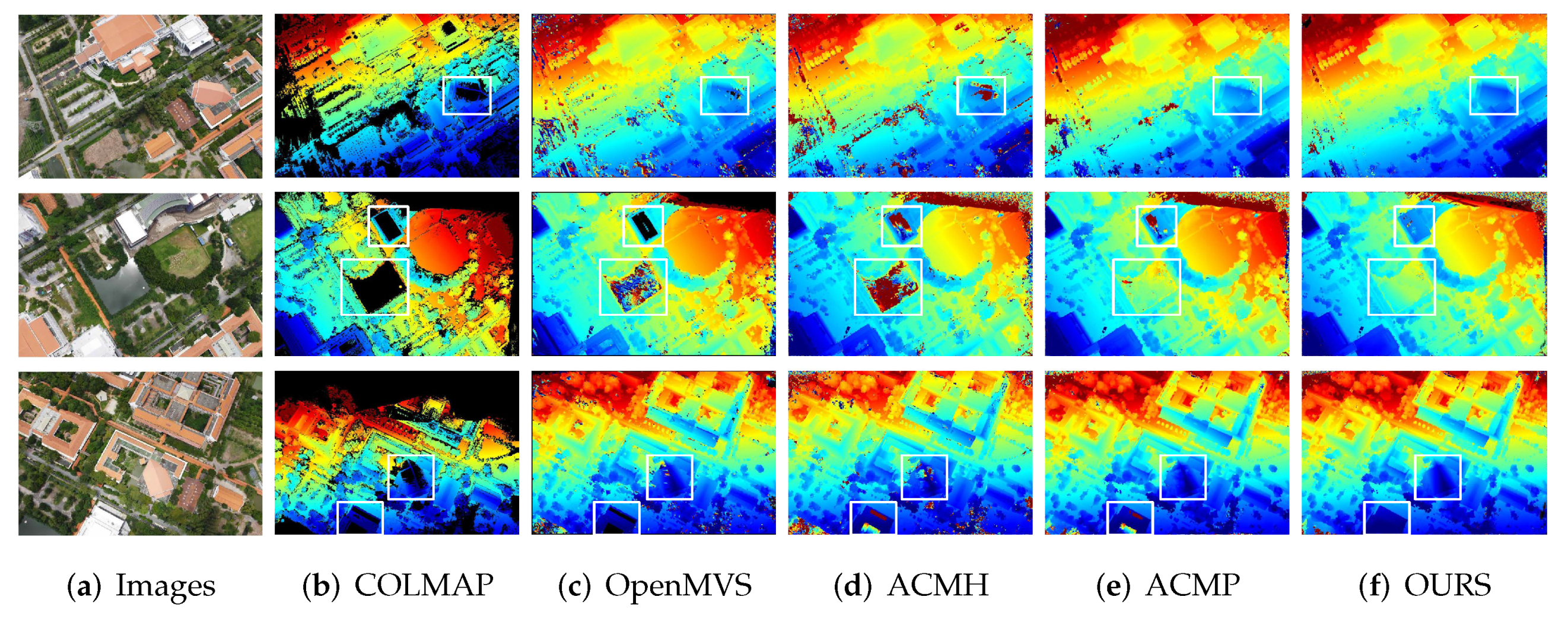
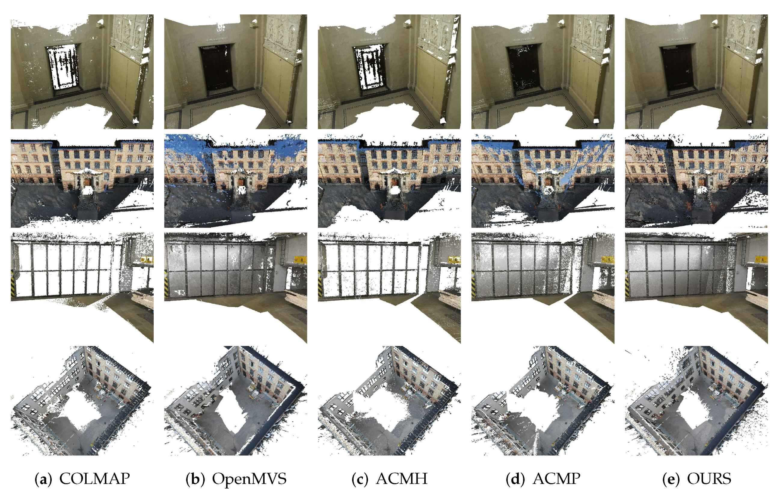
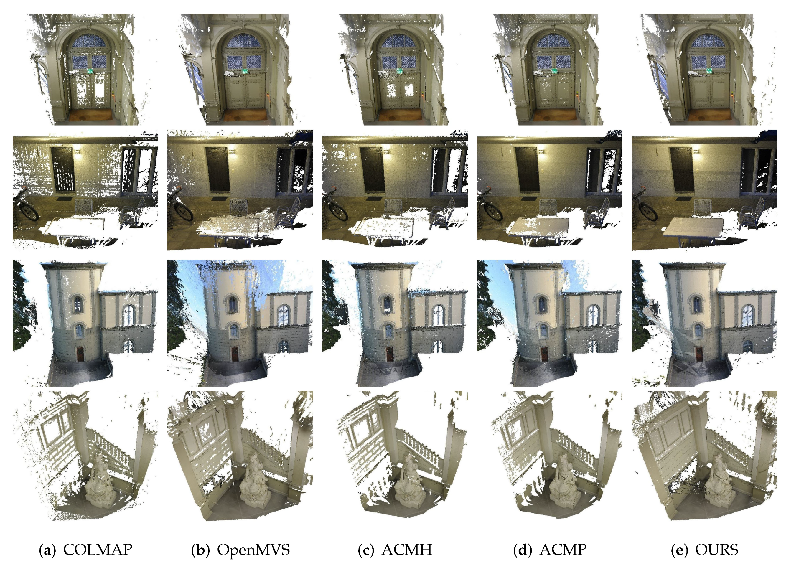
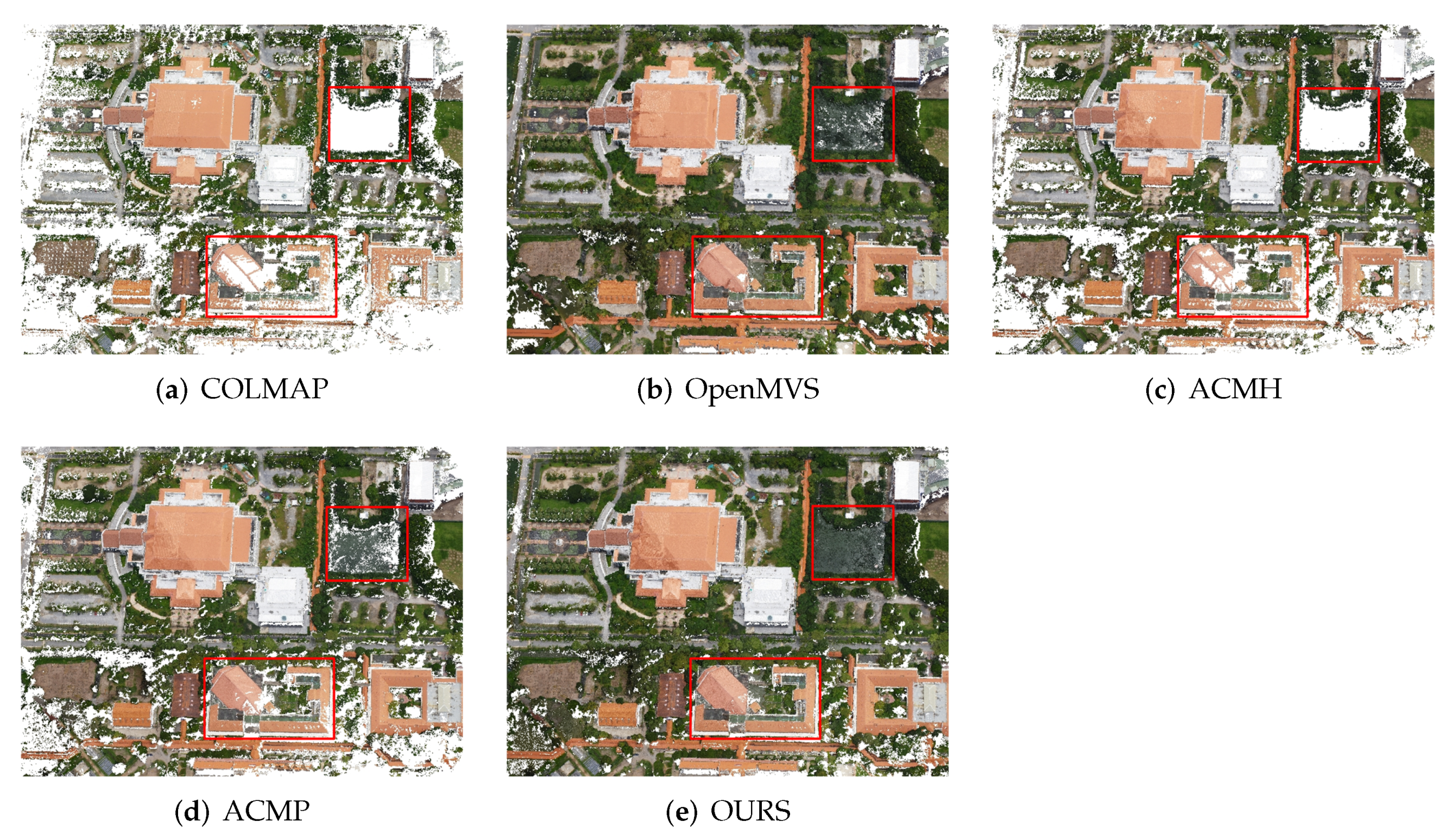
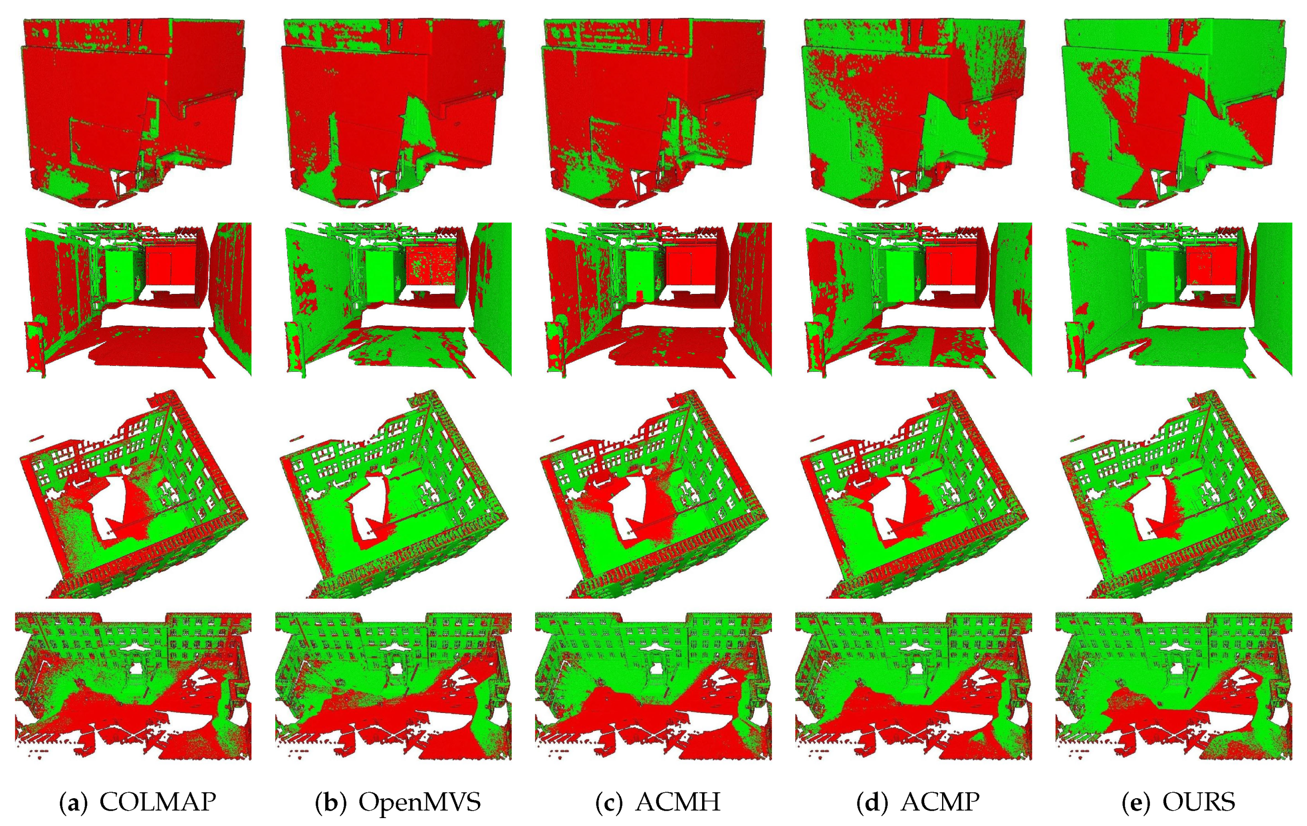
5.3. Qualification
5.4. Ablation Study
5.5. Time Evaluation
6. Conclusions
Author Contributions
Funding
Data Availability Statement
Conflicts of Interest
References
- Xu, Z.; Liu, Y.; Shi, X.; Wang, Y.; Zheng, Y. MARMVS: Matching Ambiguity Reduced Multiple View Stereo for Efficient Large Scale Scene Reconstruction. In Proceedings of the 2020 IEEE/CVF Conference on Computer Vision and Pattern Recognition (CVPR), Seattle, WA, USA, 13–19 June 2020; pp. 5980–5989. [Google Scholar] [CrossRef]
- Zhou, L.; Zhang, Z.; Jiang, H.; Sun, H.; Bao, H.; Zhang, G. DP-MVS: Detail Preserving Multi-View Surface Reconstruction of Large-Scale Scenes. Remote Sens. 2021, 13, 4569. [Google Scholar] [CrossRef]
- Zhang, Q.; Luo, S.; Wang, L.; Feng, J. CNLPA-MVS: Coarse-Hypotheses Guided Non-Local PatchMatch Multi-View Stereo. J. Comput. Sci. Technol. 2021, 36, 572–587. [Google Scholar] [CrossRef]
- Xu, Q.; Kong, W.; Tao, W.; Pollefeys, M. Multi-Scale Geometric Consistency Guided and Planar Prior Assisted Multi-View Stereo. IEEE Trans. Pattern Anal. Mach. Intell. 2023, 45, 4945–4963. [Google Scholar] [CrossRef] [PubMed]
- Bleyer, M.; Rhemann, C.; Rother, C. PatchMatch Stereo-Stereo Matching with Slanted Support Windows. In Proceedings of the British Machine Vision Conference (BMVC), Dundee, UK, 29 August–2 September 2011; pp. 14.1–14.11. [Google Scholar] [CrossRef]
- Shen, S. Accurate Multiple View 3D Reconstruction Using Patch-Based Stereo for Large-Scale Scenes. IEEE Trans. Image Process. 2013, 22, 1901–1914. [Google Scholar] [CrossRef] [PubMed]
- Cernea, D. OpenMVS: Multi-View Stereo Reconstruction Library. Available online: https://cdcseacave.github.io/openMVS (accessed on 4 August 2022).
- Fuhrmann, S.; Langguth, F.; Goesele, M. MVE—A Multi-View Reconstruction Environment. In Proceedings of the Eurographics Workshop on Graphics & Cultural Heritage, Darmstadt, Germany, 6–8 October 2014. [Google Scholar]
- Zhu, Z.; Stamatopoulos, C.; Fraser, C.S. Accurate and occlusion-robust multi-view stereo. ISPRS J. Photogramm. Remote Sens. 2015, 109, 47–61. [Google Scholar] [CrossRef]
- Galliani, S.; Lasinger, K.; Schindler, K. Massively Parallel Multiview Stereopsis by Surface Normal Diffusion. In Proceedings of the 2015 IEEE International Conference on Computer Vision (ICCV), Santiago, Chile, 7–13 December 2015; pp. 873–881. [Google Scholar] [CrossRef]
- Kuhn, A.; Hirschmüller, H.; Scharstein, D.; Mayer, H. A TV Prior for High-Quality Scalable Multi-View Stereo Reconstruction. Int. J. Comput. Vis. 2016, 124, 2–17. [Google Scholar] [CrossRef]
- Kang, S.B.; Szeliski, R.; Chai, J. Handling occlusions in dense multi-view stereo. In Proceedings of the 2001 IEEE Computer Society Conference on Computer Vision and Pattern Recognition, CVPR 2001, Kauai, HI, USA, 8–14 December 2001; Volume 1, p. I. [Google Scholar] [CrossRef]
- Strecha, C.; Fransens, R.; Van Gool, L. Combined Depth and Outlier Estimation in Multi-View Stereo. In Proceedings of the 2006 IEEE Computer Society Conference on Computer Vision and Pattern Recognition (CVPR’06), New York, NY, USA, 17–22 June 2006; Volume 2, pp. 2394–2401. [Google Scholar] [CrossRef]
- Zheng, E.; Dunn, E.; Jojic, V.; Frahm, J.M. PatchMatch Based Joint View Selection and Depthmap Estimation. In Proceedings of the 2014 IEEE Conference on Computer Vision and Pattern Recognition, Columbus, OH, USA, 23–28 June 2014; pp. 1510–1517. [Google Scholar] [CrossRef]
- Schnberger, J.L.; Zheng, E.; Pollefeys, M.; Frahm, J.M. Pixelwise View Selection for Unstructured Multi-View Stereo. In Proceedings of the European Conference on Computer Vision (ECCV), Amsterdam, The Netherlands, 11–14 October 2016. [Google Scholar]
- Romanoni, A.; Matteucci, M. TAPA-MVS: Textureless-Aware PAtchMatch Multi-View Stereo. In Proceedings of the 2019 IEEE/CVF International Conference on Computer Vision (ICCV), Seoul, Republic of Korea, 27 October–2 November 2019. [Google Scholar]
- Kuhn, A.; Lin, S.; Erdler, O. Plane Completion and Filtering for Multi-View Stereo Reconstruction. In Proceedings of the GCPR, Dortmund, Germany, 10–13 September 2019. [Google Scholar]
- Xu, Q.; Tao, W. Planar Prior Assisted PatchMatch Multi-View Stereo. In Proceedings of the AAAI Conference on Artificial Intelligence, New York, NY, USA, 7–12 February 2020; Volume 34, pp. 12516–12523. [Google Scholar]
- Yan, S.; Peng, Y.; Wang, G.; Lai, S.; Zhang, M. Weakly Supported Plane Surface Reconstruction via Plane Segmentation Guided Point Cloud Enhancement. IEEE Access 2020, 8, 60491–60504. [Google Scholar] [CrossRef]
- Huang, N.; Huang, Z.; Fu, C.; Zhou, H.; Xia, Y.; Li, W.; Xiong, X.; Cai, S. A Multi-View Stereo Algorithm Based on Image Segmentation Guided Generation of Planar Prior for Textureless Regions of Artificial Scenes. IEEE J. Sel. Top. Appl. Earth Obs. Remote Sens. 2023, 16, 3676–3696. [Google Scholar] [CrossRef]
- Stathopoulou, E.K.; Battisti, R.; Cernea, D.; Georgopoulos, A.; Remondino, F. Multiple View Stereo with quadtree-guided priors. ISPRS J. Photogramm. Remote Sens. 2023, 196, 197–209. [Google Scholar] [CrossRef]
- Xu, Q.; Tao, W. Multi-Scale Geometric Consistency Guided Multi-View Stereo. In Proceedings of the 2019 IEEE/CVF Conference on Computer Vision and Pattern Recognition (CVPR), Long Beach, CA, USA, 15–20 June 2019. [Google Scholar]
- Seitz, S.; Curless, B.; Diebel, J.; Scharstein, D.; Szeliski, R. A Comparison and Evaluation of Multi-View Stereo Reconstruction Algorithms. In Proceedings of the 2006 IEEE Computer Society Conference on Computer Vision and Pattern Recognition (CVPR’06), New York, NY, USA, 17–22 June 2006; Volume 1, pp. 519–528. [Google Scholar] [CrossRef]
- Goesele, M.; Curless, B.; Seitz, S. Multi-View Stereo Revisited. In Proceedings of the 2006 IEEE Computer Society Conference on Computer Vision and Pattern Recognition (CVPR’06), Seattle, WA, USA, 14–19 June 2006; Volume 2, pp. 2402–2409. [Google Scholar] [CrossRef]
- Kostrikov, I.; Horbert, E.; Leibe, B. Probabilistic Labeling Cost for High-Accuracy Multi-view Reconstruction. In Proceedings of the 2014 IEEE Conference on Computer Vision and Pattern Recognition, Washington, DC, USA, 23–28 June 2014; pp. 1534–1541. [Google Scholar] [CrossRef]
- Hiep, V.H.; Keriven, R.; Labatut, P.; Pons, J.P. Towards high-resolution large-scale multi-view stereo. In Proceedings of the 2009 IEEE Conference on Computer Vision and Pattern Recognition, Miami, FL, USA, 20–25 June 2009; pp. 1430–1437. [Google Scholar] [CrossRef]
- Cremers, D.; Kolev, K. Multiview Stereo and Silhouette Consistency via Convex Functionals over Convex Domains. IEEE Trans. Pattern Anal. Mach. Intell. 2011, 33, 1161–1174. [Google Scholar] [CrossRef]
- Lhuillier, M.; Quan, L. A quasi-dense approach to surface reconstruction from uncalibrated images. IEEE Trans. Pattern Anal. Mach. Intell. 2005, 27, 418–433. [Google Scholar] [CrossRef] [PubMed]
- Furukawa, Y.; Ponce, J. Accurate, Dense, and Robust Multiview Stereopsis. IEEE Trans. Pattern Anal. Mach. Intell. 2010, 32, 1362–1376. [Google Scholar] [CrossRef]
- Strecha, C.; Fransens, R.; Van Gool, L. Wide-baseline stereo from multiple views: A probabilistic account. In Proceedings of the 2004 IEEE Computer Society Conference on Computer Vision and Pattern Recognition, CVPR 2004, Washington, DC, USA, 27 June–2 July 2004; Volume 1, p. I. [Google Scholar] [CrossRef]
- Liao, J.; Fu, Y.; Yan, Q.; Xiao, C. Pyramid Multi-View Stereo with Local Consistency. Comput. Graph. Forum 2019, 38, 335–346. [Google Scholar] [CrossRef]
- Jung, W.K.; Han, J.k. Depth Map Refinement Using Super-Pixel Segmentation in Multi-View Systems. In Proceedings of the 2021 IEEE International Conference on Consumer Electronics (ICCE), Las Vegas, NV, USA, 10–12 January 2021; pp. 1–5. [Google Scholar] [CrossRef]
- Wei, M.; Yan, Q.; Luo, F.; Song, C.; Xiao, C. Joint bilateral propagation upsampling for unstructured multi-view stereo. Vis. Comput. 2019, 35, 797–809. [Google Scholar] [CrossRef]
- Yodokawa, K.; Ito, K.; Aoki, T.; Sakai, S.; Watanabe, T.; Masuda, T. Outlier and Artifact Removal Filters for Multi-View Stereo. In Proceedings of the 2018 25th IEEE International Conference on Image Processing (ICIP), Athens, Greece, 7–10 October 2018; pp. 3638–3642. [Google Scholar] [CrossRef]
- Egnal, G.; Mintz, M.; Wildes, R.P. A stereo confidence metric using single view imagery with comparison to five alternative approaches. Image Vis. Comput. 2004, 22, 943–957. [Google Scholar] [CrossRef]
- Pfeiffer, D.; Gehrig, S.; Schneider, N. Exploiting the Power of Stereo Confidences. In Proceedings of the 2013 IEEE Conference on Computer Vision and Pattern Recognition, Portland, OR, USA, 23–28 June 2013; pp. 297–304. [Google Scholar] [CrossRef]
- Seki, A.; Pollefeys, M. Patch Based Confidence Prediction for Dense Disparity Map. In Proceedings of the British Machine Vision Conference (BMVC), York, UK, 19–22 September 2016; pp. 23.1–23.13. [Google Scholar] [CrossRef]
- Li, Z.; Zuo, W.; Wang, Z.; Zhang, L. Confidence-Based Large-Scale Dense Multi-View Stereo. IEEE Trans. Image Process. 2020, 29, 7176–7191. [Google Scholar] [CrossRef]
- Li, Z.; Zhang, X.; Wang, K.; Jiang, H.; Wang, Z. High accuracy and geometry-consistent confidence prediction network for multi-view stereo. Comput. Graph. 2021, 97, 148–159. [Google Scholar] [CrossRef]
- Kuhn, A.; Sormann, C.; Rossi, M.; Erdler, O.; Fraundorfer, F. DeepC-MVS: Deep Confidence Prediction for Multi-View Stereo Reconstruction. In Proceedings of the 2020 International Conference on 3D Vision (3DV), Fukuoka, Japan, 25–28 November 2020; pp. 404–413. [Google Scholar]
- Wang, Y.; Guan, T.; Chen, Z.; Luo, Y.; Luo, K.; Ju, L. Mesh-Guided Multi-View Stereo With Pyramid Architecture. In Proceedings of the 2020 IEEE/CVF Conference on Computer Vision and Pattern Recognition (CVPR), Seattle, WA, USA, 13–19 June 2020; pp. 2036–2045. [Google Scholar] [CrossRef]
- Stathopoulou, E.E.K.; Remondino, F. Semantic photogrammetry—Boosting image-based 3D reconstruction with semantic labeling. Int. Arch. Photogramm. Remote Sens. Spat. Inf. Sci. 2019, 42, 685–690. [Google Scholar] [CrossRef]
- Stathopoulou, E.K.; Remondino, F. Multi view stereo with semantic priors. arXiv 2020, arXiv:2007.02295,. [Google Scholar] [CrossRef]
- Stathopoulou, E.K.; Battisti, R.; Cernea, D.; Remondino, F.; Georgopoulos, A. Semantically Derived Geometric Constraints for MVS Reconstruction of Textureless Areas. Remote Sens. 2021, 13, 1053. [Google Scholar] [CrossRef]
- Barnes, C.; Shechtman, E.; Finkelstein, A.; Goldman, D.B. PatchMatch: A randomized correspondence algorithm for structural image editing. ACM Trans. Graph. 2009, 28, 24. [Google Scholar] [CrossRef]
- Delaunay, B. Sur la sphère vide. A la mémoire de Georges Voronoï. Bull. De L’académie Des Sci. De L’urss. Cl. Des Sci. Mathématiques Et Na 1934, 6, 793–800. [Google Scholar]
- Liba, O.; Movshovitz-Attias, Y.; Cai, L.; Pritch, Y.; Tsai, Y.T.; Chen, H.; Eban, E.; Barron, J.T. Sky Optimization: Semantically aware image processing of skies in low-light photography. In Proceedings of the 2020 IEEE/CVF Conference on Computer Vision and Pattern Recognition Workshops (CVPRW), Seattle, WA, USA, 14–19 June 2020; pp. 2230–2238. [Google Scholar] [CrossRef]
- Schöps, T.; Schönberger, J.L.; Galliani, S.; Sattler, T.; Schindler, K.; Pollefeys, M.; Geiger, A. A Multi-View Stereo Benchmark with High-Resolution Images and Multi-Camera Videos. In Proceedings of the Conference on Computer Vision and Pattern Recognition (CVPR), Honolulu, HI, USA, 21–26 July 2017. [Google Scholar]


| Parameter | Meaning | Value |
|---|---|---|
| constant of geometric confidence | ||
| constant of depth confidence | ||
| constant of normal confidence | ||
| constant of cost confidence | ||
| K | best K neighboring views | 2 |
| constant of patch confidence | ||
| confidence threshold | ||
| constant of confidence constraint in multiview matching cost | ||
| threshold of view weight | ||
| the strictest depth difference | ||
| the strictest normal angle | ||
| the strictest geometry error |
| Method | All | Indoor | Outdoor | ||||||
|---|---|---|---|---|---|---|---|---|---|
| Acc. | Comp. | Acc. | Comp. | Acc. | Comp. | ||||
| Gipuma [10] | 36.38 | 86.47 | 24.91 | 35.80 | 89.25 | 24.61 | 37.07 | 83.23 | 25.26 |
| COLMAP [15] | 67.66 | 91.85 | 55.13 | 66.76 | 95.01 | 52.90 | 68.70 | 88.16 | 57.73 |
| ACMH [22] | 70.71 | 88.94 | 61.59 | 70.00 | 92.62 | 59.22 | 71.54 | 84.65 | 64.36 |
| OpenMVS [7] | 76.15 | 78.44 | 74.92 | 76.82 | 81.39 | 73.91 | 75.37 | 74.99 | 76.09 |
| ACMP [18] | 79.79 | 90.12 | 72.15 | 80.53 | 92.30 | 72.25 | 78.94 | 87.58 | 72.03 |
| CLD-MVS [38] | 79.35 | 82.75 | 77.36 | 81.23 | 87.22 | 77.29 | 77.16 | 77.54 | 77.45 |
| QAPM [21] | 78.47 | 80.43 | 77.50 | 80.22 | 84.34 | 77.43 | 76.43 | 75.86 | 77.59 |
| OURS | 82.64 | 86.66 | 79.39 | 85.03 | 88.52 | 82.13 | 79.86 | 84.48 | 76.19 |
| Method | All | Indoor | Outdoor | ||||||
|---|---|---|---|---|---|---|---|---|---|
| Acc. | Comp. | Acc. | Comp. | Acc. | Comp. | ||||
| Gipuma [10] | 45.18 | 84.44 | 34.91 | 41.86 | 86.33 | 31.44 | 55.16 | 78.78 | 45.30 |
| COLMAP [15] | 73.01 | 91.97 | 62.98 | 70.41 | 91.95 | 59.65 | 80.81 | 92.04 | 72.98 |
| ACMH [22] | 75.89 | 89.34 | 68.62 | 73.93 | 91.14 | 64.81 | 81.77 | 83.96 | 80.03 |
| OpenMVS [7] | 79.77 | 81.98 | 78.54 | 78.33 | 82.00 | 75.92 | 84.09 | 81.93 | 86.41 |
| ACMP [18] | 81.51 | 90.54 | 75.58 | 80.57 | 90.60 | 74.23 | 84.36 | 90.35 | 79.62 |
| CLD-MVS [38] | 82.31 | 83.18 | 82.73 | 81.65 | 82.64 | 82.35 | 84.29 | 84.79 | 83.86 |
| QAPM [21] | 80.88 | 82.59 | 79.95 | 79.50 | 82.59 | 77.39 | 85.03 | 82.58 | 87.64 |
| OURS | 85.76 | 86.17 | 85.71 | 85.29 | 85.54 | 85.46 | 87.17 | 88.05 | 86.46 |
| Method | Score | Accuracy | Completeness |
|---|---|---|---|
| Baseline | 72.77 | 90.65 | 62.46 |
| CGPR-MVS/C | 74.40 | 76.59 | 73.70 |
| CGPR-MVS/S | 78.41 | 85.68 | 73.40 |
| CGPR-MVS/A | 79.71 | 90.72 | 71.87 |
| CGPR-MVS | 82.64 | 86.66 | 79.39 |
| Module | Time(s) | Ratio (%) |
|---|---|---|
| depth estimation of ACMH | 18.79 | 49.70 |
| plane hypothesis confidence calculation | 2.36 | 6.24 |
| plane supplement | 3.52 | 9.31 |
| confidence-driven depth estimation | 13.14 | 34.75 |
| Total | 37.81 | - |
| Method | COLMAP | ACMM | ACMP | OURS |
|---|---|---|---|---|
| Time(s) | 129.9 | 43.0 | 23.7 | 37.8 |
Disclaimer/Publisher’s Note: The statements, opinions and data contained in all publications are solely those of the individual author(s) and contributor(s) and not of MDPI and/or the editor(s). MDPI and/or the editor(s) disclaim responsibility for any injury to people or property resulting from any ideas, methods, instructions or products referred to in the content. |
© 2023 by the authors. Licensee MDPI, Basel, Switzerland. This article is an open access article distributed under the terms and conditions of the Creative Commons Attribution (CC BY) license (https://creativecommons.org/licenses/by/4.0/).
Share and Cite
Fu, C.; Huang, N.; Huang, Z.; Liao, Y.; Xiong, X.; Zhang, X.; Cai, S. Confidence-Guided Planar-Recovering Multiview Stereo for Weakly Textured Plane of High-Resolution Image Scenes. Remote Sens. 2023, 15, 2474. https://doi.org/10.3390/rs15092474
Fu C, Huang N, Huang Z, Liao Y, Xiong X, Zhang X, Cai S. Confidence-Guided Planar-Recovering Multiview Stereo for Weakly Textured Plane of High-Resolution Image Scenes. Remote Sensing. 2023; 15(9):2474. https://doi.org/10.3390/rs15092474
Chicago/Turabian StyleFu, Chuanyu, Nan Huang, Zijie Huang, Yongjian Liao, Xiaoming Xiong, Xuexi Zhang, and Shuting Cai. 2023. "Confidence-Guided Planar-Recovering Multiview Stereo for Weakly Textured Plane of High-Resolution Image Scenes" Remote Sensing 15, no. 9: 2474. https://doi.org/10.3390/rs15092474
APA StyleFu, C., Huang, N., Huang, Z., Liao, Y., Xiong, X., Zhang, X., & Cai, S. (2023). Confidence-Guided Planar-Recovering Multiview Stereo for Weakly Textured Plane of High-Resolution Image Scenes. Remote Sensing, 15(9), 2474. https://doi.org/10.3390/rs15092474