Recent Cereal Phenological Variations under Mediterranean Conditions

Abstract

This study analyzes the temporal patterns of rainfed cereal phenology extracted from the GIMMS NDVI3g dataset in the main cereal-growing regions under a Mediterranean climate in Spain, Portugal, France and Italy during the period 1982–2022. The series before and after the beginning of the 21st century were analyzed separately. Phenological parameters were extracted using the modified dynamic threshold method, and their trends were analyzed. Correlation analyses were performed to study the relationships among these parameters and to analyze the influence of hydroclimatic variables on the start (SOS) and end (EOS) of the growing season. Results showed a temporal reversal in phenological trends between both study periods, coinciding with the global warming hiatus. In the first period (1982–2002), SOS and EOS advanced (−7.5 and −3.1 days, respectively), and the length of growing season (LOS) increased. However, during the second stage (2003–2022), SOS and EOS were delayed (7.5 and 1.7 days, respectively), and LOS decreased. Similar dynamics were observed for the influence of the hydroclimatic variables on SOS and EOS, stronger in the first period and weaker in the second. This study provides valuable information on the phenological dynamics of rainfed cereals that may be useful for their management and planning in climate change scenarios.

1. Introduction

Vegetation phenology dynamics are considered important biological indicators that reflect the cyclical and seasonal responses of ecosystems to climate and hydrological regimes [1]. In this context, global warming is an undeniable phenomenon with a significant impact on terrestrial vegetation, altering its phenological cycles [2]. Thus, an accurate characterization of phenology and monitoring of its behavior at different times are fundamental to understanding the variations in climate change impacts. This is of particular interest in water-limited areas, such as the Mediterranean, as it is one of the most vulnerable regions to climate change, and this vulnerability is likely to worsen in the future [3]. The soil moisture (SM) drought risk is projected to increase around the world, resulting in increased frequency and intensity of agricultural droughts under all climate scenarios, with the Mediterranean region being the most affected [4,5]. The Mediterranean region is characterized by water-limited conditions, where rainfed cereal cultivation predominates [6]. This increases the interest in the study of the phenological behavior of cereals under the Mediterranean climate, which could be an essential tool for better agronomic management under a global climate change scenario [7].

Crop phenological information is mainly extracted from in situ ground records and remote sensing data [8]. In situ monitoring of vegetation is mainly based on field observation methods and provides detailed and accurate information on plant development. However, this approach is limited by its spatial and temporal scales, making it impossible to detect phenological dynamics at larger spatial scales and to conduct long-term studies. Several studies used information from in situ observations for the analysis of phenological trends but recognized that the geographic extent is limited, as are long-term observations in complex environments [9,10].

However, satellite data are effective tools for monitoring land surfaces at large spatial and suitable temporal scales, which allow tracking of the phenological dynamics of vegetation over large areas [11]. The phenology obtained from satellite data is usually determined from vegetation indices (VIs), such as the normalized difference vegetation index (NDVI) or the enhanced vegetation index (EVI) [11,12,13]. Many studies have investigated the vegetation phenology using satellite sensors, including mainly the Advanced Very High Resolution Radiometer (AVHRR) [14,15], the Moderate Resolution Imaging Spectroradiometer (MODIS) [13] and the Satélite Pour l’Observation de la Terre (SPOT) [16]. In particular, the NDVI derived from the AVHRR sensor is the most widely used tool for studying the long-term phenological dynamics of vegetation at global, continental and regional scales. It is the longest NDVI time series to date and has been shown to have a good capability for long-term vegetation monitoring [17].

With the impressive advancements in remote sensing technologies, which make it possible to effectively monitor vegetation phenology, recent research on phenological trends and their responses to climate change has been performed at different scales. Various climatic factors, such as temperature, precipitation, photoperiod, etc., can influence the seasonal development of plants and the calendar of phenological phases [18,19]. Many studies have incorporated these variables into analyses of climatic impacts on phenology [20,21]. However, the use of other important factors, such as the soil water content, in phenological analyses using remote sensing data is uncommon, despite its crucial importance for crops and the impacts that agricultural drought is causing [5].

The main vegetation parameters that are extracted to monitor phenological dynamics are the start of the growing season (SOS), the end of the growing season (EOS) and the length of the growing season (LOS); the latter is calculated from the previous two parameters. Many studies have shown that prior to the 2000s, there was a general trend of advanced SOS in many regions, and different time periods and study methods were used [22,23]. However, since the start of the 2000s, several studies have suggested that the trend may have slowed [24,25] or even reversed [26,27,28]. In contrast, the overall trend of the EOS was more heterogeneous and less marked than that of the SOS, with a majority of advances [24,29] but also some delays [27]. The discrepancy in the trends of the main phenological metrics before and after the beginning of the 21st century has been attributed to the global warming hiatus [30]. However, it is still not clear how these trends evolved beyond that period and whether they have persisted in recent years, specifically in agricultural areas. Accordingly, Piao et al. [30] recommended continuous monitoring and analysis using satellite observations to verify whether and how the trends in phenological parameters will continue in the coming decades. Several studies [31,32,33] have noted that, despite the interest in detecting the phenological dynamics of cultivated plants at a regional scale, most researchers did not consider it due to the perception that it was influenced by anthropogenic activities. Thus, instead of focusing on cultivated plants, attention has been mostly focused towards phenological changes in natural vegetation. Moreover, in the few cases where cultivated plants have been considered, they were small-scale studies based on in situ field data [32]. Therefore, assessments of plant phenology covering both the periods before and after the global warming hiatus are needed, especially for cultivated plants. This would provide a more complete understanding of the temporal phenological dynamics of vegetation and would allow verification of the trends of most current phenological parameters.

This study aimed to analyze the patterns of the temporal phenological parameters of rainfed cereals based on the NDVI AVHRR data and their responses to hydroclimatic variables under Mediterranean conditions. The analysis was performed in the main cereal-growing regions with a Mediterranean climate in Spain, Portugal, France and Italy during the period from 1982 to 2022. This study provides a deep understanding of the phenological dynamics of crops as important as cereals, particularly in water-limited regions. In these environments, accurate management and yield forecasting are crucial to ensure food security and agricultural sustainability under a climate change scenario. This work can significantly contribute to inform management decisions with the aim to address future situations in water-limited regions for these key crops.

2. Materials and Methods

2.1. Study Area

In the Mediterranean region, the most common crops are rainfed cereals, with wheat and barley being the main crops [34,35]. The area is characterized by water-limited conditions, with dry, hot summers and mild, humid winters. The main cereal-growing regions under a Mediterranean climate in Spain (e.g., Castilla y León and Castilla-La Mancha, CL and CM, respectively); Portugal (e.g., Alentejo, AT); France (e.g., Occitanie, OC); and Italy (e.g., Puglia, PG), as highlighted in previous works [36,37,38,39], were selected as the study areas (Figure 1).

2.2. Data Source

2.2.1. Detection of Cereal Zones

To study rainfed cereal areas in the selected study areas (Figure 1), two databases were used to create a mask that filtered out all the areas other than the target areas. The Climate Change Initiative (CCI) Land Cover (LC) map obtained from the European Space Agency (ESA) was used to discard areas with different land cover types than cereal crops. It describes Earth’s land surface in 37 original LC classes based on the United Nations Land Cover Classification System (UN-LCCS) [40], with a spatial resolution of 300 m [41]. Additionally, the Digital Global Map of Irrigation Areas of the Food and Agriculture Organization (FAO) was used to exclude irrigated areas. It represents the global area that is equipped with irrigation at a spatial resolution of 5 arc minutes [42]. In this study, pixels with more than a 10% irrigated area and with land cover types different from those of rainfed and mosaic cropland were hidden. This mask was applied to all databases to select those pixels that only represented areas of rainfed cereal crops, assuming that cereals are the predominant crop in each region.

2.2.2. Remote Sensing Data and Processing

The normalized difference vegetation index third-generation V1.2 (NDVI3g) dataset for Global Inventory Modeling and Mapping Studies (GIMMS) was used as the remote sensing source data. It is based on corrected and calibrated measurements from the Advanced Very High Resolution Radiometer (AVHRR) that were obtained from different sensors onboard the National Oceanic and Atmospheric Association (NOAA) polar-orbiting meteorological satellites [43]. The dataset provided two NDVI values per month over 14–16 day compositing periods, with a spatial resolution of 0.0833 degrees and global coverage from 1982 to 2022.

The cubic spline interpolation method was used to obtain the daily NDVI time series, since it is one of the most common methods used for time interpolation [44,45]. Cubic spline interpolation of the data with piecewise cubic polynomials allows the NDVI curve to pass through two endpoints with their respective derivatives [45]. Additionally, for noise reduction, the NDVI time series was smoothed by calculating the moving average with a 30-day window.

2.2.3. Hydroclimatic Data

Climatic and SM data were used to analyze the relationships among phenological patterns and environmental conditions. The climate variables were obtained from the E-OBS database, which is a gridded daily Earth observation dataset over Europe belonging to the Copernicus Climate Change Service (C3S) European climate and assessment dataset [46]. The E-OBS database used, version 28.0, provides data with a spatial resolution of 0.1° × 0.1° and daily temporal resolution, with data available from January 1950 to December 2023. Climatic data were resampled into NDVI3g GIMMS grids using a majority filter. Among the set of climate variables that is provided by this database, four variables were selected for this study: accumulated precipitation (P), maximum temperature (Tmax), minimum temperature (Tmin) and relative humidity (RH). However, the latter was only used to calculate the vapor pressure deficit (VPD), which was defined for its agronomic relevance in vegetation development. The VPD (kPa) is the difference between the saturated vapor pressure (e_s) and the actual vapor pressure (e_a) and was calculated according to Equations (1)–(4) [47,48], where e^o is the saturated vapor pressure at the air temperature (kPa), and T_i is T_max or T_min (°C).

$$\mathrm{V}\mathrm{P}\mathrm{D}=e_s-e_a$$

(1)

$${\mathrm{e}}_{\mathrm{s}}=\frac{{\mathrm{e}}^{\mathrm{o}}\left({\mathrm{T}}_{\mathrm{m}\mathrm{a}\mathrm{x}}\right)+{\mathrm{e}}^{\mathrm{o}}\left({\mathrm{T}}_{\mathrm{m}\mathrm{i}\mathrm{n}}\right)}{2}$$

(2)

$${\mathrm{e}}^{\mathrm{o}}\left({\mathrm{T}}_{\mathrm{i}}\right)=0.6108\mathrm{e}\mathrm{x}\mathrm{p}\left(\frac{17.27{\mathrm{T}}_{\mathrm{i}}}{{\mathrm{T}}_{\mathrm{i}}+237.3}\right)$$

(3)

$${\mathrm{e}}_{\mathrm{a}}=\frac{RH}{100}\left(\frac{{\mathrm{e}}^{\mathrm{o}}\left({\mathrm{T}}_{\mathrm{m}\mathrm{a}\mathrm{x}}\right)+{\mathrm{e}}^{\mathrm{o}}\left({\mathrm{T}}_{\mathrm{m}\mathrm{i}\mathrm{n}}\right)}{2}\right)$$

(4)

As in the previous section, the moving averages were calculated using a 30-day window for P, Tmax, Tmin and VPD. Finally, to obtain the variables by season, the averages of each of the variables and for each pixel in each season of the year were calculated. Thus, autumn was considered to occur from September to November, winter from December to February, spring from March to May and summer from June to August.

The ERA5-Land reanalysis database was used as the SM database. It is provided by the European Centre for Medium-Range Weather Forecasts (ECMWF) in the framework of the C3S [49]. This reanalysis database has been widely validated and used [50,51,52]. The series provides SM data from 1981 to the present, with an hourly temporal resolution and a regular grid of 0.1°. The SM data were resampled into NDVI3g GIMMS grids using a majority filter. In addition, it provides the SM in three different depth layers in each pixel (0–100 cm). In this study, the SM values of the three layers at different depths were averaged at 12 am and 12 pm to determine the daily SM in the root zone (0–100 cm). As in the previous subsection, the moving averages SM were calculated with a 30-day window and then averaged for each season of the year.

2.3. Data Analyses

Figure 2 shows the general technical flow chart of this study. The three main components are: (1) data collection and preprocessing of phenological parameters, (2) data collection and preprocessing of hydroclimatic data, and (3) analysis of phenological parameters and hydroclimatic data.

2.3.1. Phenology Parameter Extraction

The identification of the phenological parameters of cereals was performed using the modified dynamic threshold method [53], which is an improved method of the original dynamic threshold method [54,55]. The time series of crop vegetation indices tend to be asymmetric; therefore, this method solves this problem by using two different amplitudes for the recovery of the SOS and EOS of crops [53]. A diagrammatic sketch of the modified dynamic threshold method is shown in Figure 3.

The agricultural year was defined as the period from the season in which the SOS occurred to the season in which the EOS occurred. In all study regions and for cereal crops, the SOS occurs in autumn, and the EOS occurs in summer of the following year [56,57,58,59,60,61]; therefore, the agricultural year was considered to extend from 1 September to 31 August of the following year. The SOS and EOS dates were retrieved at the pixel scale, and the amplitude thresholds were defined to be 20% according to the methodology used in several studies [14,20,62,63]. The calculations of SOS and EOS thresholds are summarized in Equation (5).

$$\left\{\begin{array}{c}{NDVI}_{SOS}\ge x+20\%\times a_1\\ {NDVI}_{EOS}\le b+20\%\times a_2\end{array}\right.$$

(5)

Derived from these two parameters, the LOS was calculated as the time between the SOS and EOS. In addition, the booting stage (BS) was identified as the date when the NDVI value during the crop year reached its maximum, indicating the peak of green biomass development [64,65], and the NDVI value in the BS (BV) was also determined. Finally, following the methodology of Jeong et al. [24], 10-year moving averages were calculated to remove statistical uncertainties caused by the first and last values and individual outliers in the time series for each pixel and for all identified phenological parameters.

2.3.2. Trend Analysis

The Mann–Kendall (MK) statistical test was used in the present study for the trend analyses. It is a nonparametric test used to identify trends in time-series data [66,67]. The ability of this test to detect trends has been demonstrated in many studies on the dynamics of vegetation phenology based on satellite observations [7,21,68]. In this study, the MK test was used to detect whether there were statistically significant increasing or decreasing trends in phenological parameters at the pixel scale. Under the null hypothesis of no trend H0, the MK test statistic (S) was calculated as follows:

$$S=\sum _{i=1}^{n-1}\sum _{j=i+1}^{n}sgn(x_j-x_i)$$

(6)

where

$$sgn\left(x\right)=\left\{\begin{array}{ll}1& ifx>0\\ 0& ifx=0\\ -1& ifx<0\end{array}\right.$$

(7)

For an upward trend, the S statistic is increased by +1, while it is decreased by −1 for a downward trend. The S statistics remain unchanged for a zero difference. The statistical parameter Z allows us to determine whether a trend is significant:

$$Z=\left\{\begin{array}{ll}\frac{S-1}{\sqrt{var\left(S\right)}}& ifS>0\\ 0& ifS=0\\ \frac{S+1}{\sqrt{var\left(S\right)}}& ifS<0\end{array}\right.$$

(8)

Throughout this study, a p value of 0.05 (95% confidence level) was used as the criterion for determining the statistical significance of a trend. Thus, for an absolute value of Z greater than 1.96, a significant trend is considered.

2.3.3. Correlation Analysis

Pearson’s correlation coefficients (R) were calculated at the pixel scale to analyze the relationships among the main phenological parameters (e.g., the SOS, EOS and LOS). The significance of the correlations was identified with p values at the 95% confidence level.

In addition, for the analysis of the influence of the hydroclimatic variables on the SOS and EOS parameters, the mean SOS and EOS dates were previously calculated for all the pixels of the study regions as well as for each season of the hydroclimatic variables. Subsequently, R values were calculated between each hydroclimatic variable and the main phenological parameters, SOS and EOS, with the statistical significance level set to p < 0.05. This analysis was conducted during the season in which the SOS and EOS occurred, as well as during the previous season. Therefore, for the SOS, the autumn season and summer season of the previous agricultural year were considered, while for the EOS, the summer and spring of the current agricultural year were considered.

3. Results

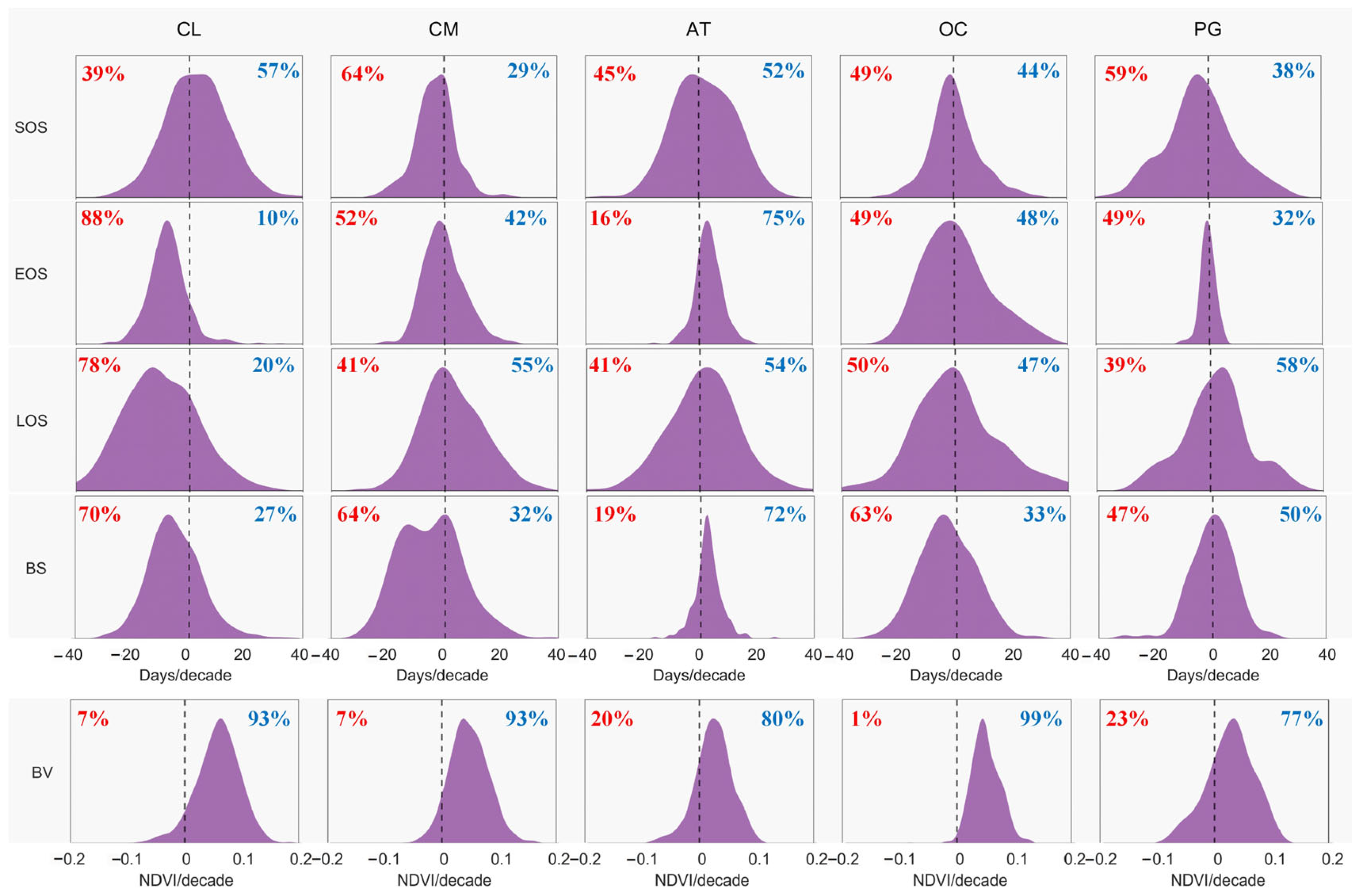
3.1. Phenological Dynamics over Decades

The initial analysis of the extracted parameters involved comparing the dates of the phenological parameters, SOS, EOS, and BS, with the LOS and BV values between the first and last decades of the study (Figure 4). Advanced dates predominated for the SOS, EOS, and BS, while the LOS increased. CM stood out, with an advanced SOS in 64% of the pixels. Regarding the EOS and LOS, the CL showed very pronounced advance and shortening, with 88% and 78%, respectively, of negative pixels. For BS, the AT showed a delay in the dates in 72% of the pixels. Conversely, for the BV, all regions showed an increase, with an average increase of 88% of the pixels.

Several authors reported changes in the phenological parameters from the 2000s onward [25,26] and associated these with the global warming hiatus [29]. In the study areas, this slowdown in global warming was also observed between the end of the 20th century and the beginning of the 21st century, as shown in Figure 5.

With the aim of studying the behavioral patterns before and after this climatic inflection, the study period was divided into two parts: the first period covered the first two decades (1982–2002), and the second period covered the last two decades (2003–2022). This approach, which involves dividing the period into two parts, namely, before and after the slowdown in global warming, has been used in other studies [2,24], although with a shorter observation period and for all types of vegetation cover.

Figure 6, Figure 7 and Figure 8 show that the decadal differences in both periods had inverse behaviors, considering the predominant pattern of each phenological parameter, except for BV, which increased in both periods. Thus, in the decadal differences of the first period, advances in the SOS and EOS and an increase in the LOS were predominantly observed (Figure 6 and Figure 7). The SOS advanced in all regions except for CL, with PG standing out for its advancement in 81% of the pixels, while for the EOS, CL showed an advancement in 75% of the pixels. The length of the phenological cycle of the PG increased in 79% of the pixels. In contrast, the differences in the decades of the second period showed delays in the SOS and EOS and decreases in the LOS (Figure 6 and Figure 7). The SOS experienced delays in all regions, with the percentages of positive pixels ranging between 52% and 67%, while the LOS decreased in all regions, with the percentages of negative pixels ranging between 56% and 64%. The EOS predominantly experienced delays, with the PG region standing out with a delay for 68% of its pixels.

BS followed the same pattern that was observed for the SOS and EOS in each period (Figure 8). During the first period, not only did the SOS and EOS advance, but they also caused a change in the phenological cycle, thus advancing the BS. In all regions, the BS advanced with an average of 76% of the pixels, except in the PG, where delayed pixels predominated, with a negligible difference of 48% compared to 45% for advanced pixels.

However, in the second period, the BS was mostly delayed, with CL occurring in 57% of the delayed pixels. In contrast, the BV showed a consistent pattern in the same direction in both periods, with average percentages of increasing pixels of 70% and 86% in the first and second periods, respectively.

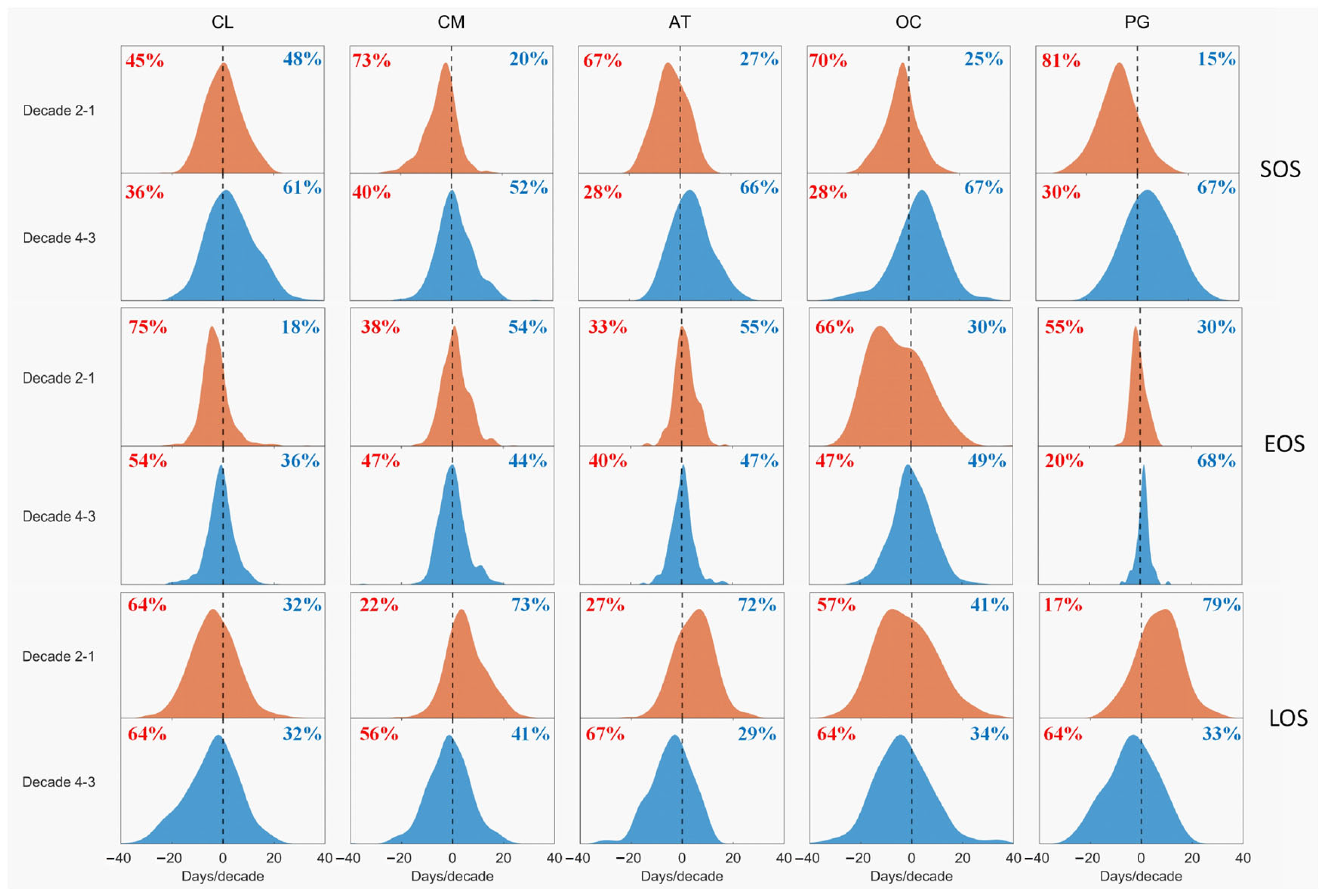
3.2. Temporal Patterns of Phenological Trends

The trends of the phenological parameters during the first and second periods are shown in

Table 1. Trends of the cereal phenological parameters, SOS, EOS, LOS, BS and BV, at the pixel scale in CL, CM, AT, OC and PG and the averages of these parameters for the two study periods. The data indicate the percentages of pixels with positive trends (P), negative trends (N), statistically significant trends p < 0.05 (S), significant positive trends (SP) and significant negative trends (SN). The highest percentages (above 50) for each parameter have been colored in red (negative trends) and blue (positive trends).

Regions	1st Period (%)					2nd Period (%)
	P	N	S	SP	SN	P	N	S	SP	SN
	SOS
CL	38	62	62	22	40	68	32	64	45	19
CM	26	73	67	13	54	66	33	65	44	21
AT	18	81	75	7	68	89	11	77	73	4
OC	21	79	70	13	57	75	25	81	64	17
PG	14	86	75	7	68	55	38	60	40	20
Average	23	76	69	12	57	71	28	69	53	16
	EOS
CL	15	85	70	8	62	39	61	59	21	38
CM	45	54	54	25	30	53	46	62	34	28
AT	48	51	59	27	32	73	27	67	51	16
OC	32	68	80	22	58	58	41	63	40	22
PG	35	65	70	25	45	75	17	72	59	13
Average	35	65	66	21	45	60	38	65	41	23
	LOS
CL	38	61	61	20	41	30	70	68	18	50
CM	66	34	55	41	14	39	60	62	23	39
AT	78	22	68	59	10	21	78	66	8	58
OC	44	55	64	27	37	32	68	62	15	47
PG	82	18	71	60	11	40	52	56	26	29
Average	62	38	64	41	23	32	66	63	18	45
	BS
CL	7	93	80	4	77	67	33	73	51	22
CM	21	78	65	10	56	38	61	82	29	54
AT	27	73	63	8	55	84	15	73	67	6
OC	16	84	74	7	67	49	51	71	34	37
PG	49	49	56	22	34	57	35	61	39	22
Average	24	75	68	10	58	59	39	72	44	28
	BV
CL	70	30	62	49	13	79	21	73	62	11
CM	58	42	62	41	21	84	16	83	73	11
AT	58	42	48	28	20	90	10	84	80	4
OC	98	2	96	94	1	92	8	93	87	6
PG	68	32	74	50	24	66	27	74	52	22
Average	70	30	68	52	16	82	17	81	71	11

, and the values of the slopes of these trends are shown in

Table 2. Slopes of the MK trends of the phenological parameters of SOS, EOS, LOS, BS and BV cereals in CL, CM, AT, OC and PG and the average of these parameters for the two study periods. Δ% indicates the percentage increase in the NDVI from the first period (1P) to the second period (2P).

Periods	Regions	SOS	EOS	LOS	BS	BV
		Days/Period				NDVI/Period	Δ% 2P-1P
1	CL	−3.2	−6.6	−3.3	−13.0	0.009
	CM	−6.1	0.0	5.6	−6.9	0.005
	AT	−10.6	−1.1	9.5	−3.7	0.004
	OC	−5.9	−7.3	−1.1	−10.6	0.021
	PG	−11.4	−0.6	10.5	−1.0	0.005
	Average	−7.5	−3.1	4.3	−7.0	0.009
2	CL	6.5	−2.0	−8.7	4.7	0.015	40
	CM	4.2	1.4	−3.3	−5.0	0.018	69
	AT	11.8	3.3	−8.7	6.6	0.020	81
	OC	9.4	2.9	−6.5	−0.6	0.020	−8
	PG	5.5	2.8	−2.6	2.4	0.012	54
	Average	7.5	1.7	−6.0	1.6	0.017	47

. Significant changes in the SOS, EOS, LOS and BS were observed in the two study periods, with an inverse pattern between them. During the first period, the SOS, EOS and BS dates tended to advance in all regions, with 76%, 65% and 75%, respectively, of the pixels showing negative trends (Table 1). The average pixels across all regions with significant trends toward advancing dates for the SOS, EOS, and BS represented nearly 55% of the total pixels. The SOS presented an average advance of 7.5 days, with the AT and PG regions experiencing the greatest advancements, exceeding 10 days (Table 2). The EOS presented an average advance of 3.1 days, while the BS advanced by 7 days, with the OC and CL regions showing the greatest advancements in both cases. In most regions, the LOS exhibited increases, although the distribution was more heterogeneous, with the CL and OC regions showing decreases due to greater advancements of the EOS than of the SOS. The average increase in the LOS across all regions was 4.3 days, with an average increase in regions with a higher percentage of positive pixels of 9 days and a mean decrease in CL and OC of 2.2 days. When contrasting regions with LOS increases and decreases, the increases in the number of days were observed to be four times greater than the decreases.

In contrast, during the second period, there was a predominant trend toward delays in the SOS, EOS, and BS dates across all regions, with 70%, 60%, and 59%, respectively, of the pixels showing positive trends (Table 1). On average, nearly 43% of the pixels across all regions exhibited significant trends toward delayed SOS, EOS, and BS dates. The SOS presented an average delay of 7.5 days, with AT and OC being the regions with the greatest advances, averaging 10.6 days (Table 2). The EOS presented an average advance of 1.7 days, and the BS presented an average advance of 1.6 days, with AT experiencing the most prolonged delay. The BS trend was more heterogeneous across all regions, as it advanced in CM and OC, while in the remaining regions, it was delayed, which was similar to what occurred in CL with the EOS, which was the only region with a higher percentage of positives. However, compared to the first period, the rate of advancement slowed, with the average advancement of the BS decreasing from 8.8 days to 2.8 days in CM and OC and from 6.6 days to 2 days in the EOS for CL. Considering all territories as a whole, the LOS presented a decreasing trend in 66% of the pixels, 68% of which were significant, with an average decrease of 6 days. BV increased in both periods, with a 47% difference in the increase between the second and first periods (Table 2). Overall, clear inverse trends in the phenological parameters were observed between the two periods, with a tendency toward delayed SOS, EOS, and BS, along with a reduction in the LOS in the latter years.

3.3. Relationships between the Phenological Parameters of Vegetation

The interrelationships among the main phenological parameters of cereals, namely, the SOS, EOS and LOS, were analyzed (

Table 3. Correlation coefficients between the phenological parameters, SOS, EOS and LOS, at the pixel scale in CL, CM, CM, AT, OC, and PG and the averages of these parameters for the two study periods. The data indicate the average R value in pixels (R), the percentage of pixels with a positive correlation (P), a negative correlation (N), a statistical significance of p < 0.05 (S), a positive significant correlation (SP) and a significant negative correlation (SN). The highest percentages (above 50) for each parameter have been colored in red (negative trends) and blue (positive trends).

Regions	1st Period						2nd Period
	P	N	S	SP	SN	R	P	N	S	SP	SN	R
	SOS—EOS
CL	57	41	52	32	20	0.09	55	45	50	28	23	0.05
CM	47	52	52	26	27	−0.02	55	44	56	33	23	0.08
AT	41	57	52	20	32	−0.09	68	32	53	43	10	0.24
OC	62	37	61	41	21	0.16	57	43	56	34	23	0.09
PG	46	52	52	24	28	−0.01	51	49	59	33	25	0.02
Average	51	48	54	28	26	0.03	57	43	55	34	21	0.09
	SOS—LOS
CL	5	95	81	0	81	−0.67	2	98	92	0	91	−0.82
CM	7	92	82	3	79	−0.65	8	92	86	4	82	−0.70
AT	0	100	95	0	95	−0.87	2	98	96	0	95	−0.84
OC	22	77	65	7	57	−0.41	6	93	84	1	83	−0.70
PG	0	100	100	0	100	−0.96	1	99	99	0	99	−0.94
Average	7	93	85	2	83	−0.71	4	96	91	1	90	−0.80
	EOS—LOS
CL	88	12	74	72	2	0.56	79	21	60	54	6	0.40
CM	90	9	78	77	1	0.64	83	17	67	62	5	0.49
AT	83	17	68	62	6	0.46	68	32	54	38	16	0.19
OC	93	7	86	84	2	0.71	83	17	67	62	5	0.50
PG	66	34	61	42	19	0.22	61	39	62	45	17	0.20
Average	84	16	73	67	6	0.52	75	25	62	52	10	0.36

). The results showed that there were no clear relationships between the SOS and EOS in either period since no marked patterns were detected in any region. The percentage of positive correlations is slightly greater than that of negative correlations, with an average percentage of significant positive correlations in all regions of approximately 55% in both the first and second periods. The mean R value in all regions was irrelevant, with values of 0.03 and 0.09 in the first and second periods, respectively.

However, when the relationships of the SOS and EOS with the LOS were analyzed, very marked patterns were observed in both periods. During the first period, there was an inverse relationship between the SOS and LOS, with an average of 93% of pixels having a negative correlation in all regions, 89% of which were significant, with an average R value of −0.71. The AT and PG regions had inverse correlations for 100% of their pixels, with 100% and 95% of the correlations being significant and with average pixel R values of −0.96 and −0.87, respectively. This indicates that the SOS advances caused an increase in the LOS, as shown in the previous section.

In the second period, relationships between the SOS and LOS were observed to be in the same direction as those in the first period but were more pronounced (Table 3). Across all regions, there were pixel percentages with inverse correlations between 92% and 99%, of which an average of 94% were significant. The average R value for the study region was −0.80. OC increased the number of pixels with a negative correlation by 16%, increased the number of pixels with an inverse and significant correlation by 26%, and increased the R value from −0.41 to −0.70. Although the relationship between the SOS and LOS remained consistent in both periods, it was slightly more pronounced in the second period. Thus, the dynamics of the SOS inversely influenced the LOS, with a stronger relationship observed in later years.

The relationships between the EOS and LOS (Table 3) were direct in both study periods, in contrast to the relationships between the SOS and LOS. In the first and second study periods, the average percentages of pixels showing direct correlations were 84% and 75%, respectively, of which 80% and 69%, respectively, were statistically significant. Across all regions, there were slight decreases in the percentages of positively correlated pixels from the first to the second period. The average R values were 0.52 and 0.36 in the first and second periods, respectively. Although this relationship remained consistent in both periods, it was slightly less pronounced in the second period. Consequently, the EOS has become less decisive in affecting the LOS in recent years. Therefore, while the SOS is becoming more determinant of the LOS, the EOS has the opposite influence. This suggests that the SOS varied more significantly than the EOS, as observed in the trend analysis.

3.4. Influence of Hydroclimatic Variables on Phenological Parameters

The analysis of the potential controls of the hydroclimatic variables on the dynamics of phenological parameters under Mediterranean conditions is shown in

Table 4. Correlation coefficients between the SOS, EOS and hydroclimatic variables during the current phenological season and the previous season for the five study regions as a whole, considering the first (1P) and second (2P) periods. p < 0.05 indicates statistical significance (*).

Variables	SOS				EOS
	Autumn		Last Summer		Summer		Spring
	1P	2P	1P	2P	1P	2P	1P	2P
P	−0.10	−0.17	0.04	0.11	−0.16	0.08	0.09	0.06
Tmax	0.27	0.53 *	−0.52 *	0.30	−0.37	0.45 *	−0.71 *	0.26
Tmin	0.08	0.03	−0.71 *	−0.14	−0.61 *	0.04	−0.58 *	−0.04
VPD	0.36	0.40	−0.45 *	0.28	−0.26	0.41	−0.54 *	0.19
SM	−0.17	−0.36	0.40	0.07	0.29	−0.04	0.50 *	−0.15

. During the first period, a distinctive pattern of statistically significant inverse correlations was observed, involving the relationships of the SOS and EOS with the Tmax, Tmin and VPD variables of the previous summer and spring, respectively. Among these, the highest R values correspond to the relationships of the SOS and EOS with Tmin and Tmax, respectively, with R values of −0.71 in both cases. During the second period, a similar pattern was also observed for both phenological parameters, with significant direct correlations of the autumn and summer Tmax values with the SOS and EOS dates, with R values of 0.53 and 0.45, respectively. Furthermore, during the spring of the first period, the EOS also showed a significant direct correlation with SM, with R values of 0.50. Similarly, during the summer of the first period, an inverse correlation between the EOS and Tmin was observed, with an R value of −0.61.

Specifically, the energy variables and SM could have played a significant role in the observed variations in the SOS and EOS during the first study period. However, in recent decades, Tmax has emerged as the variable that exerts predominant control over the dynamics of these key phenological parameters.

4. Discussion

The results revealed a clearly delineated pattern of reversal or slowdown of the phenological parameters from the beginning of the 21st century. During the first period, the SOS, EOS, and BS dates improved by averages of 7.5 days, 3.1 days, and 7 days, respectively, while the LOS increased by 4.3 days. These results are consistent with those of many previous investigations, such as Stockli and Vidale [22], which revealed a general shift toward earlier and longer growing periods in Europe, which were approximately 5.4 days/decade and 9.6 days/decade, respectively, during the period from 1982 to 2001. Piao et al. [23] reported that in China from 1982 to 1999, the SOS advanced at a rate of 7.9 days/decade, and the LOS increased by 10.16 days/decade. Furthermore, there is extensive evidence that spring events such as BS occurred increasingly earlier in the studies prior to the 2000s. For instance, Menzel et al. [69] reported an advance of 2.5 days/decade in spring phenology in Europe from 1971–2000. A study carried out by Peñuelas et al. [70] revealed that in the Mediterranean region, plants altered their cycles, with advances in phenological phases of approximately 6 days during the period from 1952 to 2000.

However, during the first decades of the 21st century, changes in the trends of phenological parameters were evident. In the present study, average delays of 7.5 days in the SOS, 1.7 days in the EOS and 1.6 days in the BS were recorded, while the LOS decreased by 6 days. Similar results were obtained by Touhami et al. [27], who detected an average delay in the SOS of 7.8 days and a decrease in the LOS of 12.8 days from 2000 to 2017 in the Mediterranean region of northeastern Tunisia. Additionally, several studies have reported trends toward delayed EOS in recent decades [71,72]. Thus, Zhu et al. [73] reported a delayed EOS of 1.6 days/decade in China. Zhang et al. [74] studied the phenology in the Northern Hemisphere and observed EOS delays of 6.3 days/decade.

The present study found strong evidence that the BV tended to increase in both periods, with average increases in the first period of 0.009 NDVI and 0.017 NDVI in the second period. The observed increase in the second period was significantly greater than that in the first period, being 47% greater. This finding is consistent with that obtained in the study of Gao et al. [75], who also identified a trend toward greening during the 1982–2020 growing season, with an average increase of 0.048 NDVI per decade. This trend showed two distinct periods, one of gradual growth before 2006 and another of drastic increase in the NDVI after 2006. De Jong et al. [76] reported a continuous increase in plant activity in Europe. Several studies have shown that the increasing rate of CO₂ fertilization caused by increasing temperatures and CO₂ levels are the main drivers of the observed greening [77,78,79]. The Intergovernmental Panel on Climate Change (IPCC) 2023 report [80] highlights that the greenhouse gas (GHG) emissions during 2010–2019 were higher than those in any previous decade. In 2019, GHG emissions were 12% higher than those in 2010 and 54% higher than those in 1990, which explains the notable increase observed in the second study period.

According to previous studies [81,82,83], an advanced SOS was associated with a longer LOS in the first study period, and this association was slightly stronger in the second period, when a delayed SOS was associated with a shorter LOS. Alternatively, it was observed that an earlier EOS was associated with a shorter LOS in the first period, but this relationship was also weaker in the second period, with a more delayed EOS associated with a longer LOS. The relationships between the SOS and LOS were slightly stronger than those between the EOS and LOS, suggesting that the SOS had a greater impact on the LOS than did the EOS; moreover, this impact was slightly more pronounced in the second period than in the first period. Additionally, a negligible relationship was found in the first period, although it was slightly more prominent in the second period between the SOS and EOS, with a positive relationship of 57% of pixels, of which 60% were significant. This finding suggests that in the second period, later SOS in autumn are usually accompanied by later EOS in summer, regardless of the summer conditions.

Changes in vegetation phenology are considered to be a consequence of adaptive responses to climatic factors [84]. Particularly in rainfed agriculture, environmental conditions determine the correct development of crops. A greater influence of the energetic variables and SM was observed during the first period in the previous season on the SOS and EOS. The discrepancy between the first and second periods coincides with the changes observed in the trends of the phenological parameters. Stronger and more significant associations were found between the first periods of the SOS and EOS in the previous summer and spring, respectively, and Tmax, Tmin, VPD and SM. More specifically, in the first period, the variables Tmax, Tmin and VPD of the previous summer were the variables that most influenced the SOS with an inverse relationship. The same pattern was observed for the EOS, except for SM aggregation, which had a direct relationship. Thus, increases in Tmax, Tmin and VPD would lead to advances in the SOS and EOS, while a decrease in SM would also advance the EOS. Several studies obtained similar results [21,85], and others have confirmed these results since at the end of the 20th century there were increases in VPD [86] and a warming of the Earth’s surface with significant increases in temperature [87]. Furthermore, in the study by Almendra-Martín et al. [88], a general decreasing trend in SM in Europe was observed. However, in the second period, the pattern that was observed in the first period changed, and only the direct relationships of Tmax in autumn and summer with the SOS and EOS, respectively, were significant. Thus, an increase in Tmax would cause delays in the SOS and EOS. In agreement with these results, del Río et al. [89] observed an increase in Tmax at a greater rate than in Tmin.

As previously observed, there is a disparity in the phenological patterns as well as in the relationships among these patterns and climatic factors between the first and second periods of this study, with the inflection point that occurred around the beginning of the 21st century. A reversal of the SOS, EOS, LOS and BV was observed after 2002. From the late 20th century until approximately 2012, the global surface temperature did not increase as rapidly as predicted by global climate models [90,91]. This slowdown in warming is known as the global warming hiatus. However, since approximately 2012, particularly more intense warming has been observed [92,93]. In the Mediterranean region under study, a reversal of the dynamics of the phenological parameters as well as a decrease in the influence of climatic variables and SM on the phenology of cereals between the first and second periods of study was obtained. This phenomenon can be attributed to the global warming hiatus, which resulted in a pause in warming around the early 2000s, as observed in most of the world [94]. Consequently, further studies in other regions are suggested to evaluate the generalizability of these findings and to better understand the impact of the global warming hiatus on crop plant phenological trends.

5. Conclusions

The results obtained in this study reveal a clear distinction between the last decades of the 20th century and the first decades of the 21st century. The trends in SOS, EOS, LOS and BS experienced significant changes between these periods. In the first period, advances in SOS, EOS and BS were observed, as well as an increase in LOS; in the second period, these trends reversed, showing delays in SOS, EOS and BS and a decrease in LOS. However, BV continued to show a steady increase in both study periods. Additionally, the SOS was more decisive than the EOS in determining the lengthening of the LOS. A greater influence of the energy climatic variables and SM was observed in the season prior to the SOS and EOS. In addition, a decrease in the influence of the energetic and SM variables on the SOS and EOS was detected throughout the study period. In the first period, the energetic variables with an inverse relationship and SM with a direct relationship during the previous season had a more significant impact on the progression of the SOS and EOS. However, in the second period, only Tmax during the SOS and EOS emergence seasons showed a direct relationship with their delays.

These findings, which are consistent with the timing of the global warming hiatus, reflect changes in the trends of phenological parameters around the beginning of the 21st century. Furthermore, they highlight the suitability of using the NDVI obtained through remote sensing to analyze the dynamics of cereal phenological parameters over time. These results extend the understanding of the changes in cereal phenology in regions under a Mediterranean climate and provide a valuable reference for understanding ecosystem responses to climate change.

Continuous monitoring of phenological parameters using remote sensing is essential for detecting long-term changes in vegetation and for better understanding the ecosystem responses to climate change. These detected phenological changes are crucial because they could impact food security, especially in regions susceptible to SM scarcity due to climate change. However, it is recommended to explore the phenology of vegetation and crops other than cereals, as well as in other areas under different environmental conditions, to determine whether this trend is generalizable. This study demonstrated the importance of understanding the phenological trends and their relationships with climate change to develop adaptation strategies and strengthen the resilience of agricultural systems to changing environmental conditions. These findings may be useful for agricultural management practices, such as sowing planning, seed and crop selection and management, as well as for developing strategies and strengthening the resilience of agricultural systems to changing environmental conditions. Furthermore, these results provide a solid basis for future research in this field, thus contributing to the advancement of knowledge and management of agricultural systems in a constantly evolving context of climate change.

References

1. Zhang, X.; Friedl, M.A.; Schaaf, C.B.; Strahler, A.H.; Hodges, J.C.; Gao, F.; Reed, B.C.; Huete, A. Monitoring vegetation phenology using MODIS. Remote Sens. Environ. 2003, 84, 471–475. [Google Scholar] [CrossRef]
2. Zhao, J.; Zhang, H.; Zhang, Z.; Guo, X.; Li, X.; Chen, C. Spatial and temporal changes in vegetation phenology at middle and high latitudes of the Northern Hemisphere over the past three decades. Remote Sens. 2015, 7, 10973–10995. [Google Scholar] [CrossRef]
3. Gu, L.; Chen, J.; Yin, J.; Sullivan, S.C.; Wang, H.-M.; Guo, S.; Zhang, L.; Kim, J.-S. Projected increases in magnitude and socioeconomic exposure of global droughts in 1.5 and 2 °C warmer climates. Hydrol. Earth Syst. Sci. 2020, 24, 451–472. [Google Scholar] [CrossRef]
4. Tramblay, Y.; Koutroulis, A.; Samaniego, L.; Vicente-Serrano, S.M.; Volaire, F.; Boone, A.; Le Page, M.; Llasat, M.C.; Albergel, C.; Burak, S.; et al. Challenges for drought assessment in the Mediterranean region under future climate scenarios. Earth-Sci. Rev. 2020, 210, 103348. [Google Scholar] [CrossRef]
5. Benito-Verdugo, P.; Martínez-Fernández, J.; González-Zamora, Á.; Almendra-Martín, L.; Gaona, J.; Herrero-Jiménez, C.M. Impact of Agricultural Drought on Barley and Wheat Yield: A Comparative Case Study of Spain and Germany. Agriculture 2023, 13, 2111. [Google Scholar] [CrossRef]
6. Jacobsen, S.-E.; Jensen, C.R.; Liu, F. Improving crop production in the arid Mediterranean climate. Field Crop. Res. 2012, 128, 34–47. [Google Scholar] [CrossRef]
7. Jiao, F.; Liu, H.; Xu, X.; Gong, H.; Lin, Z. Trend evolution of vegetation phenology in China during the period of 1981–2016. Remote Sens. 2020, 12, 572. [Google Scholar] [CrossRef]
8. Zhan, W.; Luo, F.; Luo, H.; Li, J.; Wu, Y.; Yin, Z.; Wu, Y.; Wu, P. Time-Series-Based Spatiotemporal Fusion Network for Improving Crop Type Mapping. Remote Sens. 2024, 16, 235. [Google Scholar] [CrossRef]
9. Meng, L.; Zhou, Y.; Gu, L.; Richardson, A.D.; Peñuelas, J.; Fu, Y.; Wang, Y.; Asrar, G.R.; De Boeck, H.J.; Mao, J.; et al. Photoperiod decelerates the advance of spring phenology of six deciduous tree species under climate warming. Glob. Change Biol. 2021, 27, 2914–2927. [Google Scholar] [CrossRef]
10. Walther, G.-R.; Post, E.; Convey, P.; Menzel, A.; Parmesan, C.; Beebee, T.J.; Fromentin, J.-M.; Hoegh-Guldberg, O.; Bairlein, F. Ecological responses to recent climate change. Nature 2002, 416, 389–395. [Google Scholar] [CrossRef]
11. Liao, C.; Wang, J.; Shan, B.; Shang, J.; Dong, T.; He, Y. Near real-time detection and forecasting of within-field phenology of winter wheat and corn using Sentinel-2 time-series data. ISPRS J. Photogramm. Remote Sens. 2023, 196, 105–119. [Google Scholar] [CrossRef]
12. Kibret, K.S.; Marohn, C.; Cadisch, G. Use of MODIS EVI to map crop phenology, identify cropping systems, detect land use change and drought risk in Ethiopia—An application of Google Earth Engine. Eur. J. Remote Sens. 2020, 53, 176–191. [Google Scholar] [CrossRef]
13. Gerard, F.F.; George, C.T.; Hayman, G.; Chavana-Bryant, C.; Weedon, G.P. Leaf phenology amplitude derived from MODIS NDVI and EVI: Maps of leaf phenology synchrony for Meso-and South America. Geosci. Data J. 2020, 7, 13–26. [Google Scholar] [CrossRef]
14. You, X.; Meng, J.; Zhang, M.; Dong, T. Remote sensing based detection of crop phenology for agricultural zones in China using a new threshold method. Remote Sens. 2013, 5, 3190–3211. [Google Scholar] [CrossRef]
15. Tian, R.; Li, J.; Zheng, J.; Liu, L.; Liu, Y.; Han, W.; Wang, X. The spatial-temporal patterns of spring phenology in the temperate grasslands of China and their response mechanisms to climatic factors. J. Spat. Sci. 2024, 1–19. [Google Scholar] [CrossRef]
16. Meroni, M.; Verstraete, M.M.; Rembold, F.; Urbano, F.; Kayitakire, F. A phenology-based method to derive biomass production anomalies for food security monitoring in the Horn of Africa. Int. J. Remote Sens. 2014, 35, 2472–2492. [Google Scholar] [CrossRef]
17. Fu, Y.; He, H.S.; Zhao, J.; Larsen, D.R.; Zhang, H.; Sunde, M.G.; Duan, S. Climate and spring phenology effects on autumn phenology in the Greater Khingan Mountains, Northeastern China. Remote Sens. 2018, 10, 449. [Google Scholar] [CrossRef]
18. Gordo, O.; Sanz, J.J. Impact of climate change on plant phenology in Mediterranean ecosystems. Glob. Change Biol. 2010, 16, 1082–1106. [Google Scholar] [CrossRef]
19. Menzel, A.; Yuan, Y.; Matiu, M.; Sparks, T.; Scheifinger, H.; Gehrig, R.; Estrella, N. Climate change fingerprints in recent European plant phenology. Glob. Change Biol. 2020, 26, 2599–2612. [Google Scholar] [CrossRef]
20. Jin, H.; Jönsson, A.M.; Olsson, C.; Lindström, J.; Jönsson, P.; Eklundh, L. New satellite-based estimates show significant trends in spring phenology and complex sensitivities to temperature and precipitation at Northern European latitudes. Int. J. Biometeorol. 2019, 63, 763–775. [Google Scholar] [CrossRef]
21. Yuan, M.; Wang, L.; Lin, A.; Liu, Z.; Qu, S. Variations in land surface phenology and their response to climate change in Yangtze River basin during 1982–2015. Theor. Appl. Climatol. 2019, 137, 1659–1674. [Google Scholar] [CrossRef]
22. Stöckli, R.; Vidale, P.L. European plant phenology and climate as seen in a 20-Year AVHRR land-surface parameter dataset. Int. J. Remote Sens. 2004, 25, 3303–3330. [Google Scholar] [CrossRef]
23. Piao, S.; Fang, J.; Zhou, L.; Ciais, P.; Zhu, B. Variations in satellite-derived phenology in China’s temperate vegetation. Glob. Chang. Biol. 2006, 12, 672–685. [Google Scholar] [CrossRef]
24. Jeong, S.-J.; HO, C.-H.; GIM, H.-J.; Brown, M.E. Phenology shifts at start vs. end of growing season in temperate vegetation over the Northern Hemisphere for the period 1982–2008. Glob. Chang. Biol. 2011, 17, 2385–2399. [Google Scholar] [CrossRef]
25. Cong, N.; Wang, T.; Nan, H.; Ma, Y.; Wang, X.; Myneni, R.B.; Piao, S. Changes in satellite-derived spring vegetation green-up date and its linkage to climate in China from 1982 to 2010: A multimethod analysis. Glob. Chang. Biol. 2013, 19, 881–891. [Google Scholar] [CrossRef]
26. Fu, Y.H.; Piao, S.; Op de Beeck, M.; Cong, N.; Zhao, H.; Zhang, Y.; Menzel, A.; Janssens, I.A. Recent spring phenology shifts in western Central Europe based on multiscale observations. Glob. Ecol. Biogeogr. 2014, 23, 1255–1263. [Google Scholar] [CrossRef]
27. Touhami, I.; Moutahir, H.; Assoul, D.; Bergaoui, K.; Aouinti, H.; Bellot, J.; Andreu, J.M. Multi-year monitoring land surface phenology in relation to climatic variables using MODIS-NDVI time-series in Mediterranean forest, Northeast Tunisia. Acta Oecol. 2022, 114, 103804. [Google Scholar] [CrossRef]
28. Zhang, R.; Zhou, Y.; Hu, T.; Sun, W.; Zhang, S.; Wu, J.; Wang, H. Detecting the Spatiotemporal Variation of Vegetation Phenology in Northeastern China Based on MODIS NDVI and Solar-Induced Chlorophyll Fluorescence Dataset. Sustainability 2023, 15, 6012. [Google Scholar] [CrossRef]
29. Zhu, W.; Tian, H.; Xu, X.; Pan, Y.; Chen, G.; Lin, W. Extension of the growing season due to delayed autumn over mid and high latitudes in North America during 1982–2006. Glob. Ecol. Biogeogr. 2012, 21, 260–271. [Google Scholar] [CrossRef]
30. Piao, S.; Liu, Q.; Chen, A.; Janssens, I.A.; Fu, Y.; Dai, J.; Liu, L.; Lian, X.; Shen, M.; Zhu, X. Plant phenology and global climate change: Current progresses and challenges. Glob. Chang. Biol. 2019, 25, 1922–1940. [Google Scholar] [CrossRef]
31. Guo, J.; Hu, Y. Spatiotemporal Variations in Satellite-Derived Vegetation Phenological Parameters in Northeast China. Remote Sens. 2022, 14, 705. [Google Scholar] [CrossRef]
32. Ren, S.; An, S. Temporal Pattern Analysis of Cropland Phenology in Shandong Province of China Based on Two Long-Sequence Remote Sensing Data. Remote Sens. 2021, 13, 4071. [Google Scholar] [CrossRef]
33. Measho, S.; Li, F.; Chen, G.; Hirwa, H. Characterizing Cropland Patterns Across North-East Africa Using Time Series Vegetation Indices. J. Geophys. Res. Biogeosci. 2023, 128, e2022JG007075. [Google Scholar] [CrossRef]
34. Savin, R.; Cossani, C.M.; Dahan, R.; Ayad, J.Y.; Albrizio, R.; Todorovic, M.; Karrou, M.; Slafer, G.A. Intensifying cereal management in dryland Mediterranean agriculture: Rainfed wheat and barley responses to nitrogen fertilisation. Eur. J. Agron. 2022, 137, 126518. [Google Scholar] [CrossRef]
35. Mefleh, M. Cereals of the Mediterranean region: Their origin, breeding history and grain Quality Traits. In Cereal-Based Foodstuffs: The Backbone of Mediterranean Cuisine; Boukid, F., Ed.; Springer International Publishing: Cham, Switzerland, 2021; pp. 1–18. ISBN 978-3-030-69228-5. [Google Scholar]
36. MAPA. Anuario de Estadística; Ministerio de Agricultura Pesca y Alimentación (MAPA): Madrid, Spain, 2023. [Google Scholar]
37. Stoate, C.; Borralho, R.; Araújo, M. Factors affecting corn bunting Miliaria calandra abundance in a Portuguese agricultural landscape. Agric. Ecosyst Environ. 2000, 77, 219–226. [Google Scholar] [CrossRef]
38. García-León, D.; López-Lozano, R.; Toreti, A.; Zampieri, M. Local-scale cereal yield forecasting in Italy: Lessons from different statistical models and spatial aggregations. Agronomy 2020, 10, 809. [Google Scholar] [CrossRef]
39. Statistique Agricole Annuelle 2022 et Nouvelles Séries 2010–2022. DRAAF Occitanie. Available online: https://draaf.occitanie.agriculture.gouv.fr/statistique-agricole-annuelle-2022-et-nouvelles-series-2010-2022-a7672.html (accessed on 12 April 2024).
40. Di Gregorio, A. Land Cover Classification System: Classification Concepts and User Manual: Software Version 2; Food and Agriculture Organization of the United Nations (FAO): Rome, Italy, 2005; ISBN 92-5-105327-8. [Google Scholar]
41. Defourny, P.; Kirches, G.; Brockmann, C.; Boettcher, M.; Peters, M.; Bontemps, S.; Lamarche, C.; Schlerf, M.; Santoro, M. Land Cover CCI: Product User Guide Version 2; European Space Agency (ESA): Louvain-la-Neuve, Belgium, 2012. [Google Scholar]
42. Siebert, S.; Henrich, V.; Frenken, K.; Burke, J. Update of the Digital Global Map of Irrigation Areas to Version 5; Food and Agriculture Organization of the United Nations (FAO): Rome, Italy, 2013. [Google Scholar]
43. Pinzon, J.E.; Pak, E.W.; Tucker, C.J.; Bhatt, U.S.; Frost, G.V.; Macander, M.J. Glob. Vegetation Greenness (NDVI) from AVHRR GIMMS-3G+, 1981–2022; ORNL DAAC: Oak Ridge, TN, USA, 2023. [Google Scholar] [CrossRef]
44. Wolberg, G.; Alfy, I. Monotonic cubic spline interpolation. In Proceedings of the Computer Graphics International, Canmore, AB, Canada, 7–11 June 1999; ISBN 0-7695-0185-0. [Google Scholar]
45. Talebi, H.; Samadianfard, S.; Valizadeh Kamran, K. Estimation of daily reference evapotranspiration implementing satellite image data and strategy of ensemble optimization algorithm of stochastic gradient descent with multilayer perceptron. Environ. Dev. Sustain. 2023. [Google Scholar] [CrossRef]
46. Bandhauer, M.; Isotta, F.; Lakatos, M.; Lussana, C.; Båserud, L.; Izsák, B.; Szentes, O.; Tveito, O.E.; Frei, C. Evaluation of daily precipitation analyses in E-OBS (V19.0e) and ERA5 by comparison to regional high-resolution datasets in European regions. Int. J. Climatol. 2022, 42, 727–747. [Google Scholar] [CrossRef]
47. Yoder, R.E.; Odhiambo, L.O.; Wright, W.C. Effects of vapor-pressure deficit and net-irradiance calculation methods on accuracy of standardized Penman-Monteith equation in a humid climate. J. Irrig. Drain. Eng. 2005, 131, 228–237. [Google Scholar] [CrossRef]
48. Allen, R.G.; Pereira, L.S.; Raes, D.; Smith, M. Crop Evapotranspiration: Guidelines for Computing Crop Requirements; FAO Irrigation and Drainage Paper, 56; FAO: Rome, Italy, 1998. [Google Scholar]
49. Muñoz-Sabater, J.; Dutra, E.; Agustí-Panareda, A.; Albergel, C.; Arduini, G.; Balsamo, G.; Boussetta, S.; Choulga, M.; Harrigan, S.; Hersbach, H.; et al. ERA5-Land: A state-of-the-art global reanalysis dataset for land applications. Earth Syst. Sci. Data 2021, 13, 4349–4383. [Google Scholar] [CrossRef]
50. González-Zamora, Á.; Almendra-Martín, L.; de Luis, M.; Gaona, J.; Martínez-Fernández, J. How Are Pine Species Responding to Soil Drought and Climate Change in the Iberian Peninsula? Forests 2023, 14, 1530. [Google Scholar] [CrossRef]
51. Almendra-Martín, L.; Martínez-Fernández, J.; Piles, M.; González-Zamora, Á.; Benito-Verdugo, P.; Gaona, J. Influence of atmospheric patterns on soil moisture dynamics in Europe. Sci. Total Environ. 2022, 846, 157537. [Google Scholar] [CrossRef]
52. Gaona, J.; Benito-Verdugo, P.; Martínez-Fernández, J.; González-Zamora, Á.; Almendra-Martín, L.; Herrero-Jiménez, C.M. Soil Moisture Outweighs Climatic Factors in Critical Periods for Rainfed Cereal Yields: An Analysis in Spain. Agriculture 2022, 12, 533. [Google Scholar] [CrossRef]
53. Huang, X.; Liu, J.; Zhu, W.; Atzberger, C.; Liu, Q. The Optimal Threshold and Vegetation Index Time Series for Retrieving Crop Phenology Based on a Modified Dynamic Threshold Method. Remote Sens. 2019, 11, 2725. [Google Scholar] [CrossRef]
54. White, M.A.; Thornton, P.E.; Running, S.W. A continental phenology model for monitoring vegetation responses to interannual climatic variability. Glob. Biogeochem. Cycles 1997, 11, 217–234. [Google Scholar] [CrossRef]
55. Jonsson, P.; Eklundh, L. Seasonality extraction by function fitting to time-series of satellite sensor data. IEEE Trans. Geosci. Remote Sens. 2002, 40, 1824–1832. [Google Scholar] [CrossRef]
56. MAPA. Calendario de Siembra, Recolección y Comercialización; Ministerio de Agricultura Pesca y Alimentación (MAPA): Madrid, Spain, 2023. [Google Scholar]
57. Morais, T.G.; Silva, C.; Jebari, A.; Álvaro-Fuentes, J.; Domingos, T.; Teixeira, R.F. A proposal for using process-based soil models for land use Life cycle impact assessment: Application to Alentejo, Portugal. J. Clean. Prod. 2018, 192, 864–876. [Google Scholar] [CrossRef]
58. Manfron, G.; Delmotte, S.; Busetto, L.; Hossard, L.; Ranghetti, L.; Brivio, P.A.; Boschetti, M. Estimating inter-annual variability in winter wheat sowing dates from satellite time series in Camargue, France. Int. J. Appl. Earth Obs. Geoinf. 2017, 57, 190–201. [Google Scholar] [CrossRef]
59. Yang, C.; Fraga, H.; van Ieperen, W.; Santos, J.A. Assessing the impacts of recent-past climatic constraints on potential wheat yield and adaptation options under Mediterranean climate in southern Portugal. Agric. Syst. 2020, 182, 102844. [Google Scholar] [CrossRef]
60. Ventrella, D.; Stellacci, A.M.; Castrignano, A.; Charfeddine, M.; Castellini, M. Effects of crop residue management on winter durum wheat productivity in a long term experiment in Southern Italy. Eur. J. Agron. 2016, 77, 188–198. [Google Scholar] [CrossRef]
61. Meyer, N.; Bergez, J.-E.; Constantin, J.; Belleville, P.; Justes, E. Cover crops reduce drainage but not always soil water content due to interactions between rainfall distribution and management. Agric. Water Manag. 2020, 231, 105998. [Google Scholar] [CrossRef]
62. Ersi, C.; Bayaer, T.; Bao, Y.; Bao, Y.; Yong, M.; Lai, Q.; Zhang, X.; Zhang, Y. Comparison of Phenological Parameters Extracted from SIF, NDVI and NIRv Data on the Mongolian Plateau. Remote Sens. 2023, 15, 187. [Google Scholar] [CrossRef]
63. Kern, A.; Marjanović, H.; Barcza, Z. Spring vegetation green-up dynamics in Central Europe based on 20-Year Long MODIS NDVI data. Agric. For. Meteorol. 2020, 287, 107969. [Google Scholar] [CrossRef]
64. Pan, Z.; Huang, J.; Zhou, Q.; Wang, L.; Cheng, Y.; Zhang, H.; Blackburn, G.A.; Yan, J.; Liu, J. Mapping crop phenology using NDVI time-series derived from HJ-1 A/B data. Int. J. Appl. Earth Obs. Geoinf. 2015, 34, 188–197. [Google Scholar] [CrossRef]
65. Benedetti, R.; Rossini, P. On the use of NDVI profiles as a tool for agricultural statistics: The case study of wheat yield estimate and forecast in Emilia Romagna. Remote Sens. Environ. 1993, 45, 311–326. [Google Scholar] [CrossRef]
66. Mann, H.B. Nonparametric Tests against Trend. Econometrica 1945, 13, 245–259. [Google Scholar] [CrossRef]
67. Kendall, M.G. Rank Correlation Methods; Griffin: London, UK, 1948. [Google Scholar]
68. Karkauskaite, P.; Tagesson, T.; Fensholt, R. Evaluation of the Plant Phenology Index (PPI), NDVI and EVI for Start-of-Season Trend Analysis of the Northern Hemisphere Boreal Zone. Remote Sens. 2017, 9, 485. [Google Scholar] [CrossRef]
69. Menzel, A.; Sparks, T.H.; Estrella, N.; Koch, E.; Aasa, A.; Ahas, R.; Alm-Kübler, K.; Bissolli, P.; Braslavská, O.; Briede, A.; et al. European phenological response to climate change matches the warming pattern. Glob. Chang. Biol. 2006, 12, 1969–1976. [Google Scholar] [CrossRef]
70. Peñuelas, J.; Filella, I.; Comas, P. Changed plant and animal life cycles from 1952 to 2000 in the Mediterranean region. Glob. Chang. Biol. 2002, 8, 531–544. [Google Scholar] [CrossRef]
71. Fan, J.; Min, J.; Yang, Q.; Na, J.; Wang, X. Spatial-Temporal Relationship Analysis of Vegetation Phenology and Meteorological Parameters in an Agro-Pasture Ecotone in China. Remote Sens. 2022, 14, 5417. [Google Scholar] [CrossRef]
72. Liu, Y.; Shen, X.; Zhang, J.; Wang, Y.; Wu, L.; Ma, R.; Lu, X.; Jiang, M. Variation in Vegetation Phenology and Its Response to Climate Change in Marshes of Inner Mongolian. Plants 2023, 12, 2072. [Google Scholar] [CrossRef] [PubMed]
73. Zhu, E.; Fang, D.; Chen, L.; Qu, Y.; Liu, T. The Impact of Urbanization on Spatial–Temporal Variation in Vegetation Phenology: A Case Study of the Yangtze River Delta, China. Remote Sens. 2024, 16, 914. [Google Scholar] [CrossRef]
74. Zhang, J.; Zhao, J.; Wang, Y.; Zhang, H.; Zhang, Z.; Guo, X. Comparison of land surface phenology in the Northern Hemisphere based on AVHRR GIMMS3g and MODIS datasets. ISPRS J. Photogramm. Remote Sens. 2020, 169, 1–16. [Google Scholar] [CrossRef]
75. Gao, W.; Zheng, C.; Liu, X.; Lu, Y.; Chen, Y.; Wei, Y.; Ma, Y. NDVI-based vegetation dynamics and their responses to climate change and human activities from 1982 to 2020: A case study in the Mu Us Sandy Land, China. Ecol. Indic. 2022, 137, 108745. [Google Scholar] [CrossRef]
76. De Jong, R.; Verbesselt, J.; Zeileis, A.; Schaepman, M.E. Shifts in Global Vegetation Activity Trends. Remote Sens. 2013, 5, 1117–1133. [Google Scholar] [CrossRef]
77. Mishra, N.B.; Mainali, K.P. Greening and browning of the Himalaya: Spatial patterns and the role of climatic change and human drivers. Sci. Total Environ. 2017, 587–588, 326–339. [Google Scholar] [CrossRef] [PubMed]
78. Kumar, R.; Nath, A.J.; Nath, A.; Sahu, N.; Pandey, R. Landsat-based multi-decadal spatio-temporal assessment of the vegetation greening and browning trend in the Eastern Indian Himalayan Region. Remote Sens. Appl. Soc. Environ. 2022, 25, 100695. [Google Scholar] [CrossRef]
79. Piao, S.; Yin, G.; Tan, J.; Cheng, L.; Huang, M.; Li, Y.; Liu, R.; Mao, J.; Myneni, R.B.; Peng, S.; et al. Detection and attribution of vegetation greening trend in China over the last 30 years. Glob. Chang. Biol. 2015, 21, 1601–1609. [Google Scholar] [CrossRef] [PubMed]
80. Lee, H.; Calvin, K.; Dasgupta, D.; Krinner, G.; Mukherji, A.; Thorne, P.; Trisos, C.; Romero, J.; Aldunce, P.; Barrett, K. Climate Change 2023: Synthesis Report. Contribution of Working Groups I, II and III to the Sixth Assessment Report of the Intergovernmental Panel on Climate Change; IPCC: Geneva, Switzerland, 2023; pp. 35–115. [Google Scholar] [CrossRef]
81. Julien, Y.; Sobrino, J. Global land surface phenology trends from GIMMS database. Int. J. Remote Sens. 2009, 30, 3495–3513. [Google Scholar] [CrossRef]
82. Wu, C.; Chen, J.; Gonsamo, A.; Price, D.; Black, T.; Kurz, W. Interannual variability of carbon sequestration is determined by the lag between ends of net uptake and photosynthesis: Evidence from long records of two contrasting forest stands. Agric. For. Meteorol. 2012, 164, 29–38. [Google Scholar] [CrossRef]
83. Wu, C.; Hou, X.; Peng, D.; Gonsamo, A.; Xu, S. Land surface phenology of China’s temperate ecosystems over 1999–2013: Spatial–temporal patterns, interaction effects, covariation with climate and implications for productivity. Agric. For. Meteorol. 2016, 216, 177–187. [Google Scholar] [CrossRef]
84. Hmimina, G.; Dufrêne, E.; Pontailler, J.-Y.; Delpierre, N.; Aubinet, M.; Caquet, B.; de Grandcourt, A.; Burban, B.; Flechard, C.; Granier, A.; et al. Evaluation of the potential of MODIS satellite data to predict vegetation phenology in different biomes: An investigation using ground-based NDVI measurements. Remote Sens. Environ. 2013, 132, 145–158. [Google Scholar] [CrossRef]
85. Yuan, Z.; Bao, G.; Dorjsuren, A.; Oyont, A.; Chen, J.; Li, F.; Dong, G.; Guo, E.; Shao, C.; Du, L. Climatic Constraints of Spring Phenology and Its Variability on the Mongolian Plateau From 1982 to 2021. J. Geophys. Res. Biogeosci. 2024, 129, e2023JG007689. [Google Scholar] [CrossRef]
86. Yuan, W.; Zheng, Y.; Piao, S.; Ciais, P.; Lombardozzi, D.; Wang, Y.; Ryu, Y.; Chen, G.; Dong, W.; Hu, Z.; et al. Increased atmospheric vapor pressure deficit reduces global vegetation growth. Sci. Adv. 2019, 5, eaax1396. [Google Scholar] [CrossRef] [PubMed]
87. Braganza, K.; Karoly, D.J.; Arblaster, J.M. Diurnal temperature range as an index of global climate change during the twentieth century. Geophys. Res. Lett. 2004, 31, L13217. [Google Scholar] [CrossRef]
88. Almendra-Martín, L.; Martínez-Fernández, J.; Piles, M.; González-Zamora, Á.; Benito-Verdugo, P.; Gaona, J. Analysis of soil moisture trends in Europe using rank-based and empirical decomposition approaches. Glob. Planet. Chang. 2022, 215, 103868. [Google Scholar] [CrossRef]
89. del Río, S.; Cano-Ortiz, A.; Herrero, L.; Penas, A. Recent trends in mean maximum and minimum air temperatures over Spain (1961–2006). Theor. Appl. Climatol. 2012, 109, 605–626. [Google Scholar] [CrossRef]
90. Fyfe, J.C.; Gillett, N.P.; Zwiers, F.W. Overestimated global warming over the past 20 years. Nat. Clim. Chang. 2013, 3, 767–769. [Google Scholar] [CrossRef]
91. Medhaug, I.; Stolpe, M.B.; Fischer, E.M.; Knutti, R. Reconciling controversies about the Global Warming Hiatus. Nature 2017, 545, 41–47. [Google Scholar] [CrossRef]
92. Zahradníček, P.; Brázdil, R.; Štěpánek, P.; Trnka, M. Reflections of global warming in trends of temperature characteristics in the Czech Republic, 1961–2019. Int. J. Climatol. 2021, 41, 1211–1229. [Google Scholar] [CrossRef]
93. Huang, X.; Ma, L.; Liu, T.; Sun, B.; Chen, Y.; Qiao, Z.; Liang, L. Response relationship between the abrupt temperature change-climate warming hiatus and changes in influencing factors in China. Int. J. Climatol. 2021, 41, 5178–5200. [Google Scholar] [CrossRef]
94. Kosaka, Y.; Xie, S.-P. Recent global-warming hiatus tied to equatorial Pacific surface cooling. Nature 2013, 501, 403–407. [Google Scholar] [CrossRef] [PubMed]
Figure 1. Location map of the cereal zones in the study regions: Castilla y León (CL) and Castilla La Mancha (CM) in Spain; Alentejo (AT) in Portugal; Occitanie (OC) in France; and Puglia (PG) in Italy.
Remotesensing 16 01879 g001
Figure 2. The technical flow chart of this study.
Remotesensing 16 01879 g002
Figure 3. Application of the modified dynamic threshold method on the NDVI series throughout the agricultural year to extract the phenological parameters: start (SOS), end (EOS), length (LOS) of the growing season, booting stage (BS), and the NDVI value in the BS (BV). BV is the maximum NDVI value within the growing season, “x” is the minimum NDVI value on the left side of BV and “b” is the minimum value on the right side of BV. The black arrow indicates the retrieval of the BS date from BV. “a1” denotes the difference between BV and x, while “a2” denotes the difference between BV and b; these are the amplitudes used to retrieve SOS and EOS, respectively.
Remotesensing 16 01879 g003
Figure 4. Histograms of the distributions of the start (SOS), end (EOS), length (LOS) of the growing season, booting stage (BS), and the NDVI value in the BS (BV) differences between the last (2013–2022) and first (1982–1992) decades of the study period at the pixel scale in Castilla y León (CL), Castilla La Mancha (CM), Alentejo (AT), Occitanie (OC) and Puglia (PG). Values equal to 0 are excluded from the percentages (advance, red; delay, blue).
Remotesensing 16 01879 g004
Figure 5. Average monthly mean temperature (°C) of the study regions from 1982 to 2022 and the regression lines and their equations for the period associated with the global warming hiatus (green) and the periods before (red) and after (blue).
Remotesensing 16 01879 g005
Figure 6. Spatial distribution of the differences in the start (SOS), end (EOS) and length (LOS) of the growing season, between the two decades (1993–2002 minus 1982–1992) of the first period and of the second period (2013–2022 minus 2003–2012), represented at the pixel scale in Castilla y León (CL), Castilla La Mancha (CM), Alentejo (AT), Occitanie (OC) and Puglia (PG).
Remotesensing 16 01879 g006
Figure 7. Histograms of the distributions of the differences in the start (SOS), end (EOS) and length (LOS) of the growing season between the second (1993–2002) and first (1982–1992) decade (Decade 2–1, brown) and between the fourth (2013–2022) and third (2003–2012) decade (Decade 4–3, blue), represented at the pixel scale in in Castilla y León (CL), Castilla La Mancha (CM), Alentejo (AT), Occitanie (OC) and Puglia (PG). Values equal to 0 are excluded from the percentages (advance, red; delay, blue).
Remotesensing 16 01879 g007
Figure 8. Histograms of the distribution of the differences in the booting stage (BS) and the NDVI value in the BS (BV) between the second (1993–2002) and first (1982–1992) decade (Decade 2–1, brown) and between the fourth (2013–2022) and third (2003–2012) decade (Decade 4–3, blue), represented at the pixel scale in Castilla y León (CL), Castilla La Mancha (CM), Alentejo (AT), Occitanie (OC) and Puglia (PG). Values equal to 0 are excluded from the percentages (advance, red; delay, blue).
Remotesensing 16 01879 g008