Abstract
The study focused on the prediction of the Temperature Vegetation Dryness Index (TVDI), an agricultural drought index, for a Mango orchard in Tamale, Ghana. It investigated the temporal relationship between the meteorological drought index, Standardized Precipitation Index (SPI), and TVDI. The SPI was calculated based on utilizing precipitation data from the World Meteorological Organization (WMO) database (2010–2022) and CMIP6 projected precipitation data (2023–2050) from 35 climate models representing various Shared Socioeconomic Pathway (SSP) climate change scenarios. Concurrently, TVDI was derived from Landsat 8/9 satellite imagery, validated using thermal data obtained from unmanned aerial vehicle (UAV) surveys. A comprehensive cross-correlation analysis between TVDI and SPI was conducted to identify lag times between these indices. Building on this temporal relationship, the TVDI was modeled as a function of SPI, with varying lag times as inputs to the Wavelet-Adaptive Neuro-Fuzzy Inference System (Wavelet-ANFIS). This innovative approach facilitated robust predictions of TVDI as an agricultural drought index, specifically relying on SPI as a predictor of meteorological drought occurrences for the years 2023–2050. The research outcome provides practical insights into the dynamic nature of drought conditions in the Tamale mango orchard region. The results indicate significant water stress projected for different time frames: 186 months for SSP126, 183 months for SSP245, and 179 months for both SSP370 and SSP585. This corresponds to a range of 55–57% of the projected months. These insights are crucial for formulating proactive and sustainable strategies for agricultural practices. For instance, implementing supplemental irrigation systems or crop adaptations can be effective measures. The anticipated outcomes contribute to a nuanced understanding of drought impacts, facilitating informed decision-making for agricultural planning and resource allocation.
1. Introduction
Global climate changing, especially in arid and semi-arid regions, has caused notable shifts in precipitation patterns. Consequently, this has led to changes in the occurrence of hydrological extreme events like floods or droughts, both temporally and spatially [1]. Responding appropriately to these threatening impacts requires specific measures to protect the population, increase their resilience, and support more sustainable and climate-resilient agricultural practices [2]. In this regard, the simulation and prediction of drought condition using historical data and climate change scenarios for agricultural farmland is needed. This can be done by downloading the data of Coupled Model Intercomparison Project Phase 6 (CMIP6), which is based on different shared socioeconomic pathway (SSP) scenarios of projected socioeconomic global changes up to the end of this century [3,4]. One of the major threats to agricultural productivity is drought. Drought is a multidimensional concept and categorized as a natural hazard. It is a complex phenomenon, which is difficult to monitor and define. In order to have a tangible understanding of drought, it is better to categorize different types of droughts. Then the best definition for each category can be provided. Agricultural water management studies have mostly focused on two types of droughts, meteorological and agricultural [5]. Meteorological drought occurs when there is a deficit in precipitation compared to the long-term average. Standard precipitation index (SPI) makes it possible to calculate meteorological drought base on the amount of precipitation [6]. Agricultural droughts are usually accompanied by meteorological droughts. If the available water for a crop in each stage of the development is not sufficient, the farming system will be faced with water stress and consequently the crop yields will drop and agricultural drought occurs [7,8]. Indication of water stress of plants are manifested in increased leaf temperature and decreased vegetation (leaf) water content (VWC). Thus, many studies focusing on vegetation water balance are based on land surface temperature (LST). In the past, the LST was measured by infrared thermometers, which was costly and time-consuming. Since the 1980s, remote sensing (RS) data, particularly satellite imagery, has been used for LST calculations [9]. When referring to satellite position, the term “surface” denotes anything visible from the atmosphere on the Earth’s surface. For instance, in a mango orchard, the tree canopy is regarded as a surface, therefore the Land Surface Temperature (LST) is equivalent to the leaf surface temperature [10]. In this regard, many studies developed and improved LST retrieval methods to estimate crop water stress and consequently irrigation water demands for RS data [11,12,13,14]. Furthermore, RS has been used to calculate vegetation indices (VIs) like the normalized difference vegetation index (NDVI). The relationship between NDVI and LST has been used to track crop and orchard water stress through the temperature vegetation dryness index (TVDI). The TVDI measures a combined signal of both soil moisture under trees and the leaves water status [15]. The Landsat 8 and 9 satellite platform combines multispectral and thermal band information and comes with relatively high spatial resolutions, consistency and the free availability of the data by the U.S. Geological Survey (USGS), which made these platforms especially useful for calculating TVDI information [16,17,18,19].
Various fields of science and technology have utilized data-driven computing tools such as artificial neural networks (ANNs) and fuzzy logic, for modeling purposes [20,21]. These techniques are based on ideas how information is processed in biological systems. One of the advantages of such “soft” computing methods in system modeling is getting accurate results without having well-defined nonlinear physical relations between variables [22,23]. Adaptive Neuro-Fuzzy Inference System (ANFIS) is a method that combines the advantages of both neural networks and fuzzy logic. ANFIS are a type of adaptive networks that functions like fuzzy inference systems, and are potent processing tools for solving complex problems [24,25]. Many studies have been shown that ANFIS is one of the most suitable data driven models for drought monitoring [26,27,28,29,30]. Although artificial intelligence-(AI) methods such as ANFIS and feed forward neural network (FFNN) are flexible and useful methods in meteorological simulation studies, they have some limitations with non-stationary time series data, and input/output data requires pre-processing. One way to accomplish this is using signal processing with wavelet transforms, which, in combination, lead to hybrid models known as Wavelet-ANFIS [31].
The main aim of the present study is to predict the TVDI as an agricultural drought index for a Mango orchard located in Tamale, Ghana. The research focuses on exploring the lag time between the meteorological drought index, SPI, and the TVDI. The approach involves utilizing precipitation data obtained from the World Meteorological Organization (WMO) database, which contains 18 years of monthly-observed data from 2005 to 2022. Additionally, CMIP6 projected precipitation data between 2023 and 2050 from 35 different climate models representing various SSP scenarios are included. The SPI is then calculated based on the latter data. The TVDI is calculated in the next step using Landsat 8 and 9 satellite data validated with an unmanned aerial vehicle (UAV) thermal data survey. By analyzing the cross-correlation between the TVDI and SPI, the lag time between the two indices is identified. Based on this, the TVDI is defined as a function of SPI with varying lag times as inputs to a machine learning model, Wavelet-ANFIS, i.e., the TVDI will be predicted based on SPI as an agricultural drought index for upcoming decades (2023–2050).
2. Materials and Methods
2.1. Study Area and Precipitation Data
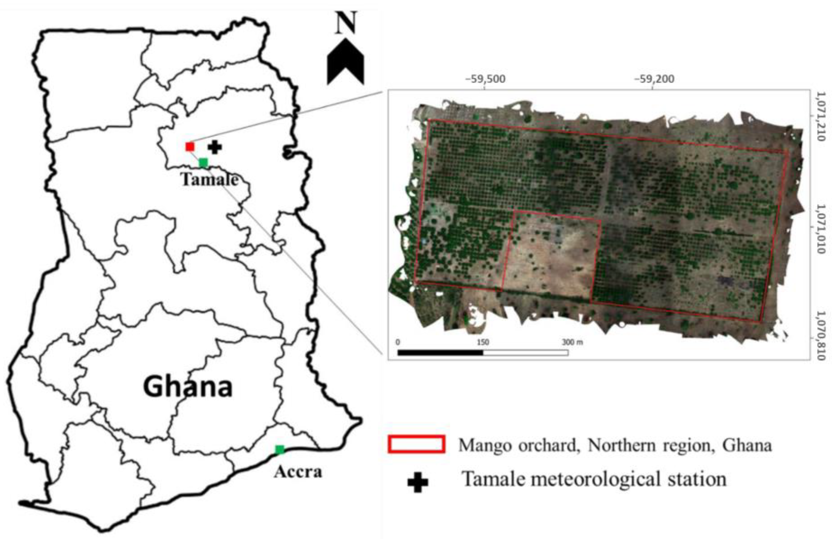
In this study, a Mango orchard located in the northern region of Ghana with the distance of about 9 km from Tamale meteorological station was selected (Figure 1). The longitude and latitude of the field center and meteorological station are 9°32′44.1″N, 0°55′58.2″W and 9°33′00.0″N, 0°51′00.0″W, respectively (path/row: 194/53 for Landsat 8 and 9 satellite images).

Figure 1.
The study area: Mango orchard northwest from Tamale (Ghana).
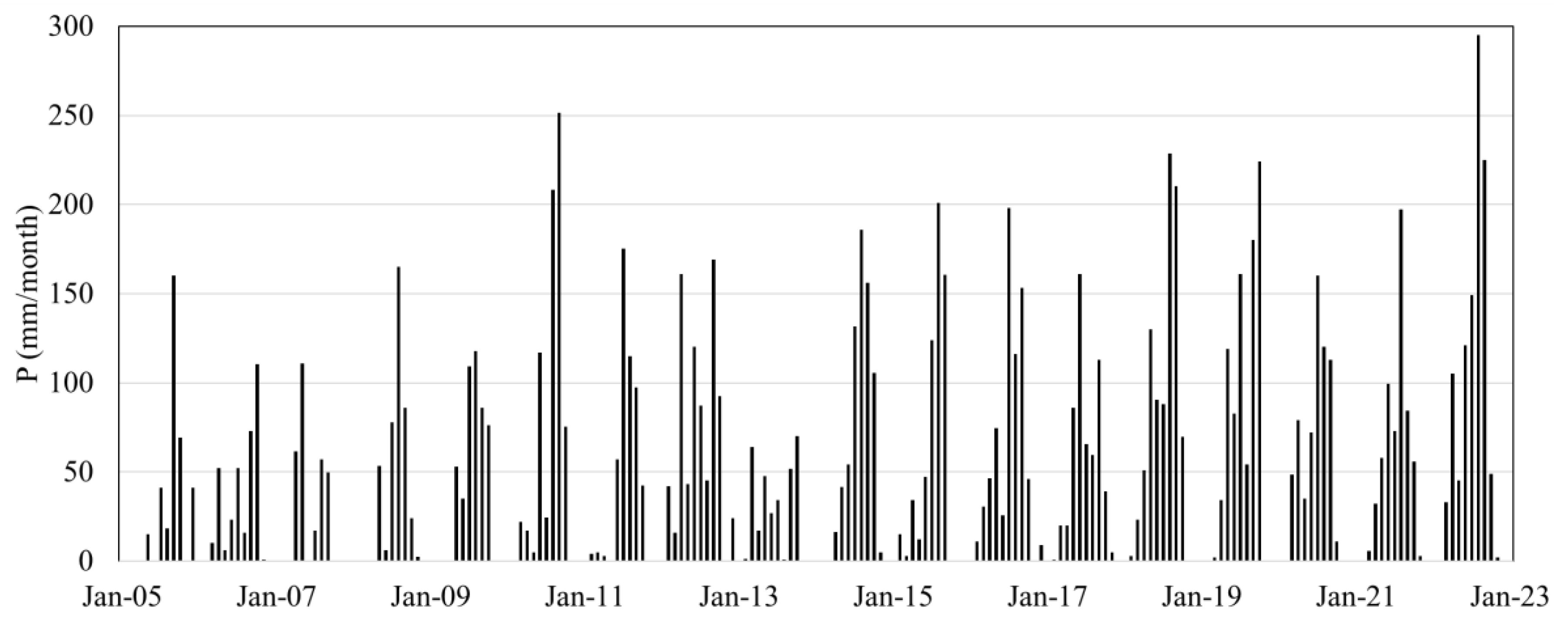
Monthly precipitation data for the time interval of January 2005 to December 2022 were obtained from SYNOP/BUFR (SYNoptic/Binary Universal Form for the Representation of meteorological data) meteorological observations, which are provided by the World Meteorological Organization (WMO) for global exchange of meteorological data between national weather services (Figure 2).

Figure 2.
Monthly precipitation (P) data for Tamale (2005–2022).
2.2. Extracting Precipitation Data for Time Interval of 2023–2050 Using CMIP6 Data
The Coupled Model Intercomparison Project Phase 6 (CMIP6) is a multi-model approach aimed at improving the prediction of climate change. It involves the coordinated use of global climate models developed by various research groups worldwide. CMIP6 provides a platform for comparing and synthesizing projections of future climate change. In total, it incorporates 35 climate models (Table 1) representing 4 different shared socioeconomic pathway (SSP) climate scenarios. These SSP based scenarios span a range from sustainable and green pathway (SSP126) to ongoing growth in emissions from fossil fuels (SSP585). SSP245 and SSP370 fall in between the two scenarios mentioned above [32].

Table 1.
The list of the complete names of the 35 models in CMIP6.
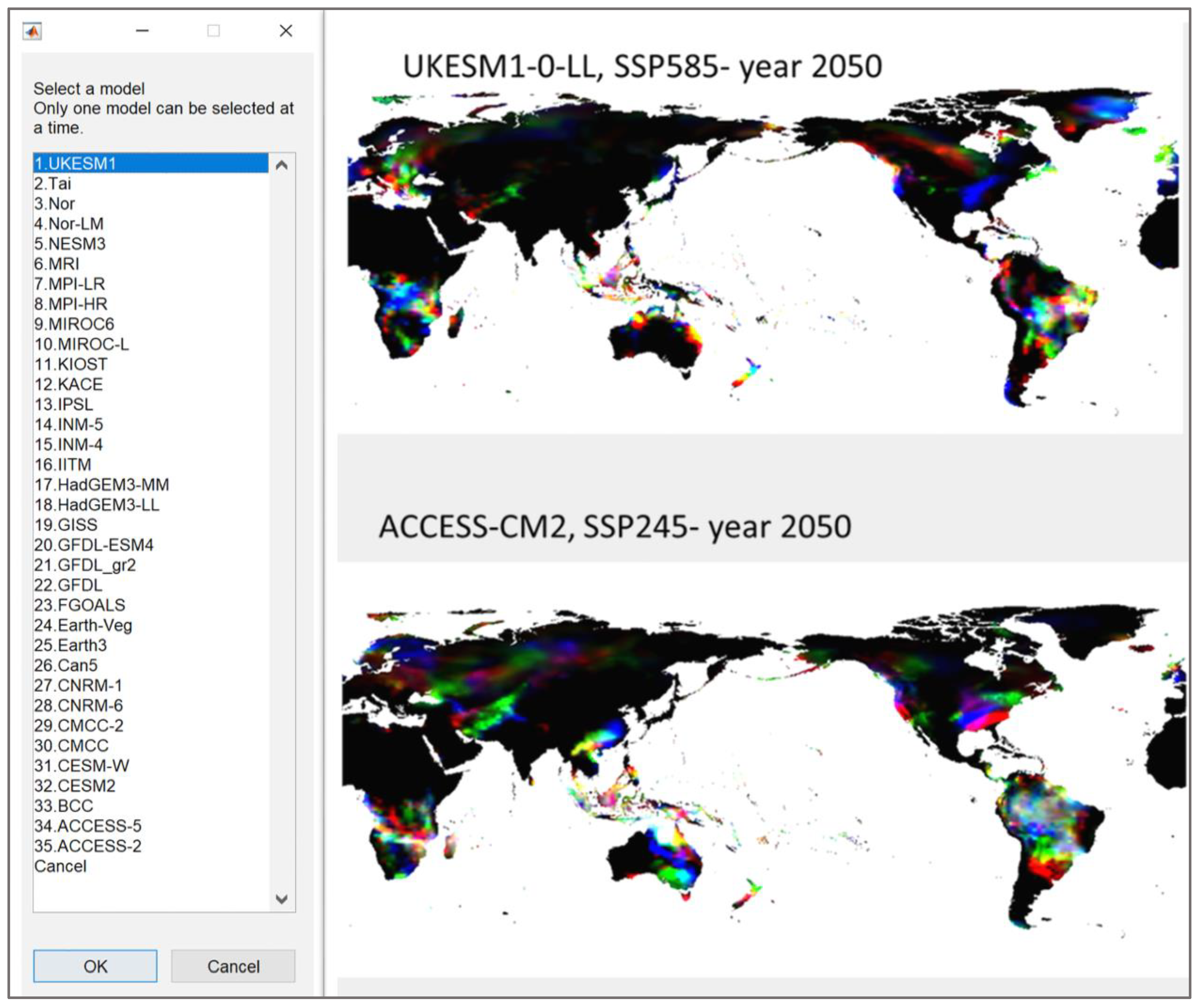
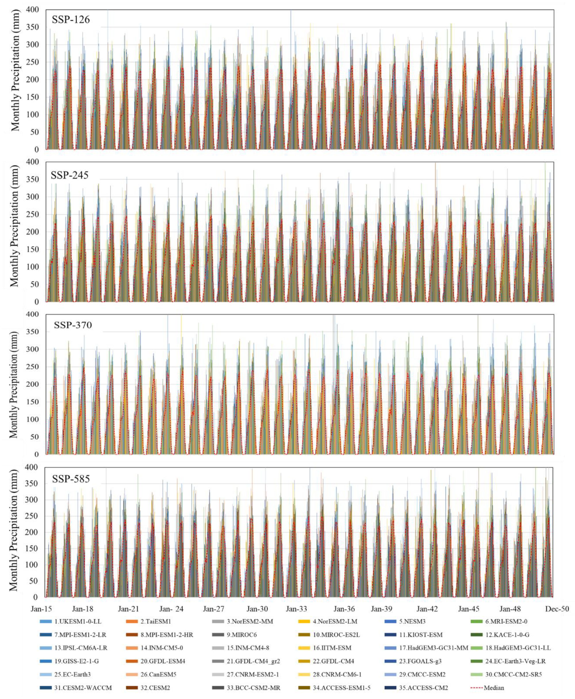
As shown in Figure 3, the climate change scenarios can be obtained from the NASA Earth Exchange Global Daily Downscaled Projections-CMIP6 (NEX-GDDP-CMIP6) archive using a GitHub repository [33]. Since the estimation of monthly meteorological drought index is needed for the present study, the time series of monthly precipitation drought for each SSP scenario has been extracted from the global climate models. To mitigate the influence of outlier data (extreme values) for each month, the median values of the 35 models have been selected to represent monthly precipitation in the study area (see Figure 4). Specifically, the median precipitation value across the 35 global climate models (GCMs) has been utilized to assess changes in monthly precipitation [34]. The median value reflects the consensus among the majority of models regarding drought, normal, or wet conditions. For instance, if at least 18 models indicate a drought condition, the median value would indicate a drought condition for each Shared Socioeconomic Pathway (SSP) scenario.

Figure 3.
List of Coupled Model Intercomparison Project Phase 6 (CMIP6) models (left) and monthly precipitation for different socioeconomic pathways of one model for december 2050 (right).

Figure 4.
The monthly precipitation values for of CMIP6 climate change scenarios for Tamale, Ghana (lat/lon: 9°32′44.1″N/0°55′58.2″W).
2.3. Landsat 8 and 9 Satellite Image Acquisition and Data Preprocessing
Landsat 8/9 satellite provides nine spectral bands based on the Operational Land Imager (OLI) sensor that covers the range from 0.45 to 2.29 μm, and two thermal bands based on the Thermal InfraRed Sensor (TIRS) sensor that work in the high infrared range of 10.0–12.5 μm. The OLI bands have a relatively high horizontal resolution of 30 m, and the frequent sweep of the satellite over the same corridor at the earth’s surface appeared in intervals of 16 days. These images are freely available through the USGS website, http://earthexplorer.usgs.gov (accessed on 21 March 2024). In total, 52 cloud-free Landsat images (39 from Landsat 8 and 13 from Landsat 9), with less than 5% cloudiness, were acquired during the time interval of 2020–2022 (Table 2).
Table 2.
Landsat 8 and 9 (L8/L9) overpass over the orchards; path/row: 194/53, Time: between 10:20 and 10:21 Local time (equal to Greenwich Mean Time).
To preprocess the satellite images for analysis, the digital numbers (DN) of the TIRS and OLI bands were transformed into spectral radiance and top-of-atmosphere (TOA) planetary reflectance. The formula below was utilized to convert the DNs to radiance [35,36].
where is the spectral radiance (W/(m2 sr µm)), is the radiance multiplicative scaling factor, is the DN value of each pixel and is the radiance additive scaling factor. TIRS data were converted from spectral radiance to brightness temperature [35,36].
where is Top of Atmosphere (TOA) brightness temperature for TIRS band (=10, 11) in Kelvin. The K coefficients are thermal conversion constants for Landsat 8/9 TIRS bands (Table 3).
Table 3.
Thermal conversion constants for Landsat 8 and 9 (L8 and L9).
The NDVI is computed by TOA planetary spectral reflectance with solar angle correction. The DNs are converted to TOA planetary reflectance by the equation below [35,36]:
where and are TOA planetary spectral reflectance with and without solar angle correction (unitless), is reflectance multiplicative scaling factor, is reflectance additive scaling factor and is solar elevation angle. and parameters in Equations (1) and (3) are extracted from metadata file obtained from satellite images downloaded from the USGS EarthExplorer.
2.4. NDVI and TVDI Calculation Using Landsat Satellite Imagery
After conversion of the DN to reflectance, the normalized difference vegetation index (NDVI) was calculated by the following equation using the red and near infrared (NIR) bands [37]
The NDVI range lies between −1 and 1. If the NDVI value is negative, it suggests the presence of water bodies or snow cover. On the other hand, if the NDVI value is greater than 0.5, it indicates the existence of dense vegetation cover [17].
In order to calculate TVDI, the land surface temperature (LST) should be determined using radiative transfer theory (RTT) equation and split-window (SW) algorithm. A simplified radiative transfer equation expresses the apparent radiance received by a sensor [38].
where radiance received by channel i (i = 10, 11) of the sensor with brightness temperature ; is the ground radiance and is the atmospheric transmittance for channel i when viewing zenith angle is . The Landsat-8 TIRS is at an altitude of 705 km with a swath width of 185 km., TIRS was treated as nadir viewing, because the maximum zenith viewing angle is not more than 7.5°. Therefore, was ignored because at that angle, the effect of the atmospheric transmittance on TIRS band is negligible. is land surface emissivity (LSE); and are down-welling and up-welling path radiance, respectively [39]. In order to retrieve LST from Landsat TIRS bands by RTT equation, split window (SW) algorithm that proposed by [40] has been used in the present study Equation (6)
where:
C and D are middle term variables:
and coefficients are determined by linear regression between intermediate parameter and . is the derivative of the Plank’s law function for band at brightness temperature [41].
As shown in the above equations the A coefficients depend on LSE () and atmospheric transmittance ().
The LSE is the ratio of radiated thermal energy by surface and a blackbody in the same temperature [9]. It can be estimated by NDVI-based emissivity method (NBEM):
where and are constant coefficients. For Landsat TIRS band 10, and are 0.973 and 0.047, respectively; and are the thresholds of soil and full vegetation pixels; and are soil and vegetation emissivity values [42]; is proportion of vegetation in mixed pixels Equation (13).
is cavity effect due to the surface roughness. It is considered zero for flat surface, otherwise the value needs to be estimated [43]:
where is a geometrical factor, which spans the range 0 to 1, and is frequently set to 0.55 [43]. The atmosphere absorbs surface spectral reflections, and the main factor affecting reflector absorption is the amount of water vapor (w) present. This quantity can be estimated by:
where is the temperature near the surface of the earth. The atmospheric transmittance () mainly depends on w. The relation between w and is shown in Table 4.
Table 4.
Relation between atmospheric transmittance factor (, i = 10, 11) and water vapor content (w) for mid-latitude atmospheric profile.
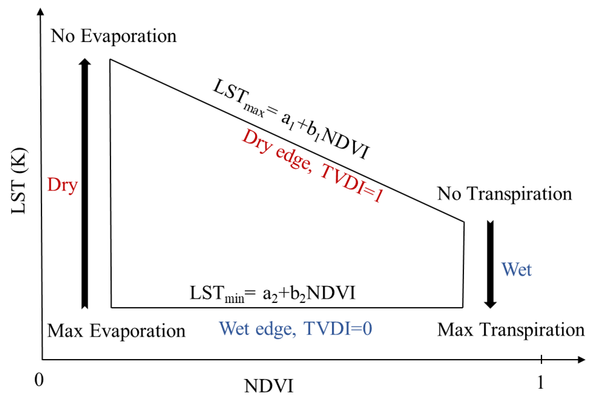
The calculated LST (Figure 5) and NDVI scatter plot produces a space with a trapezoid-like shape [45,46]. As depicted in Figure 6, every region within this space carries valuable information regarding the water content of both the canopy and soil, enabling the extraction of details about the orchard’s water status. The dry and wet edges can be leveraged to infer the water condition of the orchard. Specifically, a negative correlation between NDVI and LST can be observed in the dry edge, indicating the occurrence of water stress. Conversely, the tree is not experiencing stress in the wet edge. The TVDI, which ranges between 0 and 1, is defined as follows:
where a1 and b1 are the intercept and slope of dry edge line (Figure 6), i is the pixel number.
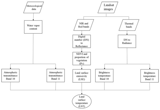
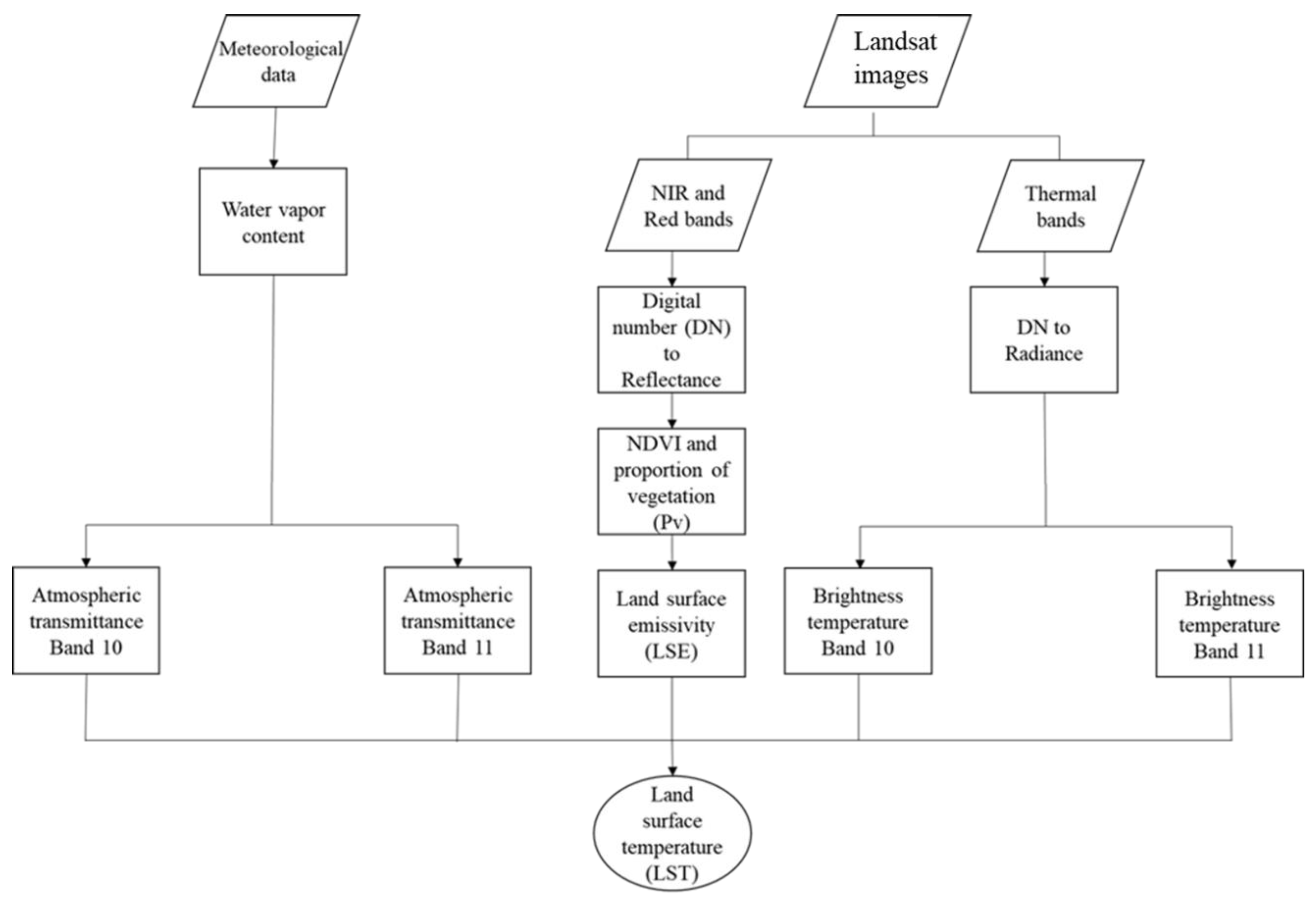
Figure 5.
Flowchart of split window (SW) algorithm.
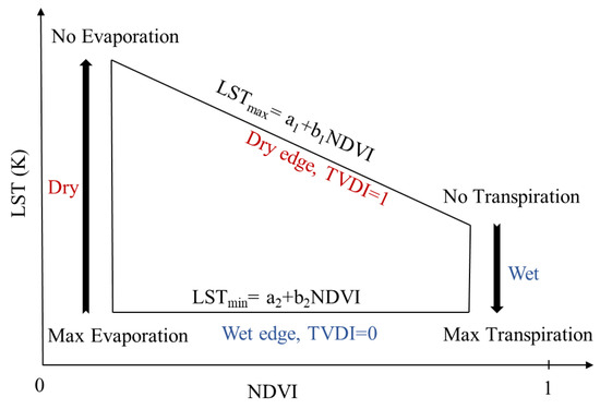
Figure 6.
Land surface temperature (LST)—NDVI trapezoidal space for temperature vegetation dryness index (TVDI [0, 1]) estimation, from [13].
2.5. Ortho Image Creation from UAV Imagery
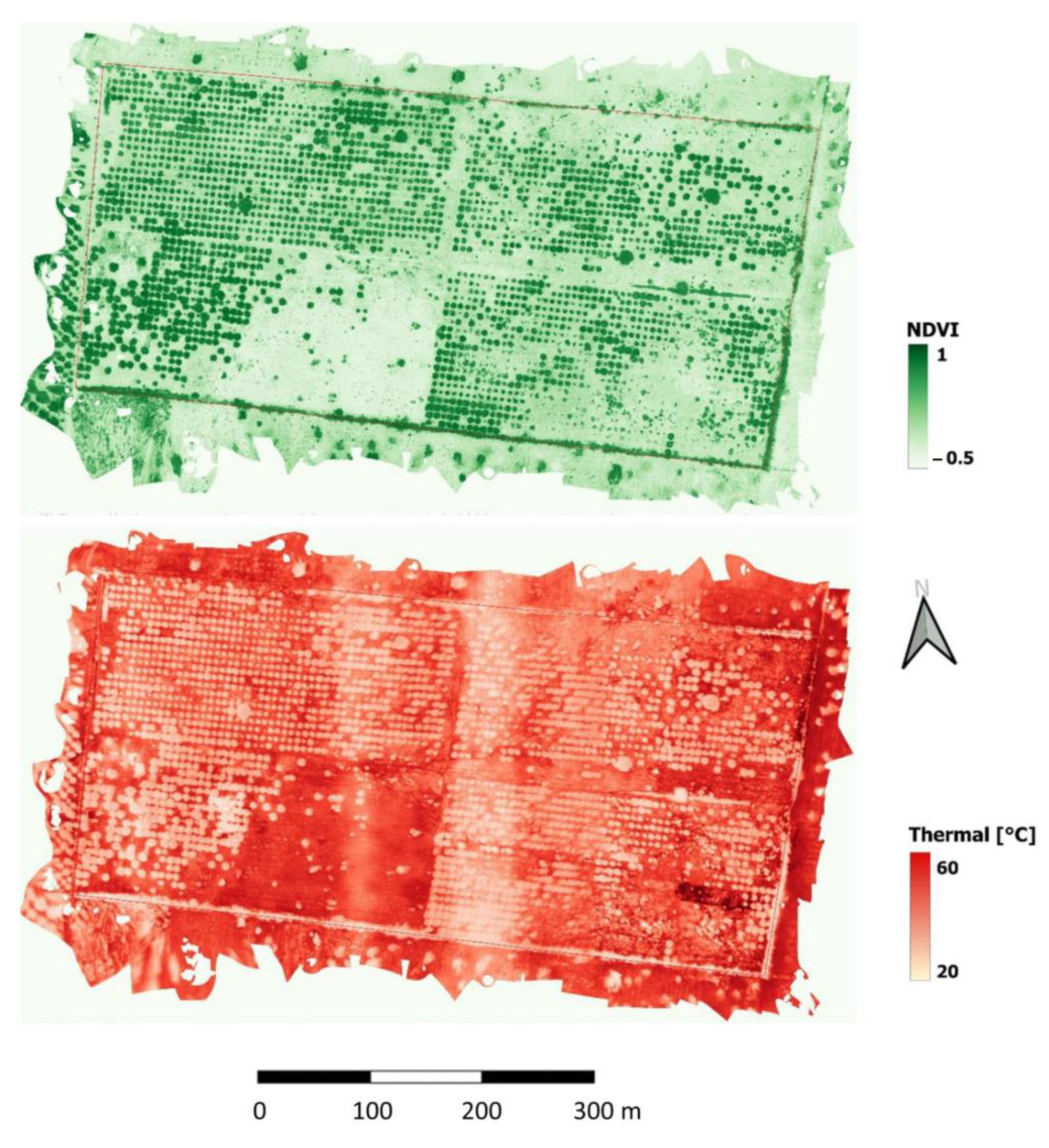
The validation of satellite-based TVDI was carried out with a UAV survey on 23 March 2023 (Figure 7). A quadrocopter (Matrice 300 RTK, DJI, China) was mounted with a combination of a multispectral and thermal camera sensor (Altum, MicaSense, Seattle, WA, USA). During the UAV survey, multispectral as well as thermal imagery data were collected from an altitude of 50 m in nadir perspective. Images were taken with over 90% forward and side overlap. Total flight distance over the site with an area of 18.7 ha was about 28.8 km and took over 3 h and 12 min. The thermal band took measurements from 8–14 µm with a focal length of 1.77 mm and a sensor resolution of 160 × 120 px. Images were stored once a second with a 33.75 cm ground sample distance.

Figure 7.
Orthoimages showing NDVI and thermal band from UAV survey completed on 19 March 2022.
From the UAV flights, 1800 multispectral and thermal images were collected. The imagery was photogrammetrically processed with structure-from-motion in Metashape (version 1.8.4, Agisoft LLC, St. Petersburg, Russia, 2020) to calculate orthoimages of the individual bands of the area. The surface temperature, measured in centi Kelvin, was transformed to °C as follows:
for which T is the thermal sensor response of the surface temperature in centi Kelvin and is the temperature transformed to °C. From the multispectral bands, the NDVI was calculated as follows:
for which NIR is the reflectance measured in the near infrared wavelengths (840 nm center with 40 nm bandwidth) and RED in the red wavelengths (668 nm center with 10 nm bandwidth) recorded by the multispectral camera.
2.6. Standard Precipitation Index (SPI)
Regarding the availability of data and the rainfed agricultural system in Tamale, Ghana, alongside the popularity of the standardized precipitation index (SPI), the SPI index was chosen over other meteorological drought indices such as Palmer drought severity Index (PDSI), percent of normal precipitation, standardized precipitation-evapotranspiration Index (SPEI), effective drought index (EDI), rainfall anomaly index (RAI) and deciles index. SPI is the most common drought index, developed by [46]. It is based on precipitation data for different time scales. In order to calculate SPI, long-term monthly precipitation data are needed. For SPI calculation, it has been assumed that the frequency distribution of precipitation data (g(x)) follows the two-parameter gamma probability distribution [46,47]:
where is precipitation accumulation; and are the shape and scale parameters of the gamma distribution; is the gamma function. To calculate the SPI, the fitted data to gamma distribution was transformed to standard normal distribution function. The SPI can be calculated for 3, 6, 12, 24 and 48-month time scales. Positive SPI values show greater precipitation than median and negative values indicate less than median precipitation. The SPI spans are between −3 to +3, because it has been transformed to the standard normal distribution. The classification of drought severity is shown in Table 5 [46].
Table 5.
SPI classification [46].
The seasonal drought in Tamale, Ghana can be classified into two categories: wet/dry seasons, which divide the year into 6-month periods, and the year divided into four seasons. Therefore, 3 and 6-month time scales has been used to calculate the SPI (SPI3 and SPI6). It is important to note that the calculated SPI is based on n-month cumulative precipitation data, which means that the precipitation accumulation in Equation (19) is calculated by adding up the precipitation from the current month, as well as the 2 (SPI3) and 5 (SPI6) preceding months.
2.7. Prediction of Agricultural Drought by a Hybrid Wavelet-ANFIS/Fuzzy C-Means (FCM) Clustering Model
To study the effects of meteorological drought on the agricultural one, a hybrid Wavelet-Adaptive Neuro-Fuzzy Inference System (ANFIS) model based on fuzzy C-means (FCM) clustering was developed, which is a data-driven input-output prediction model [31]. The following input-output prediction model for TVDI at time t, TVDIt as a function of SPI3,t-i and SPI6,t-i is used:
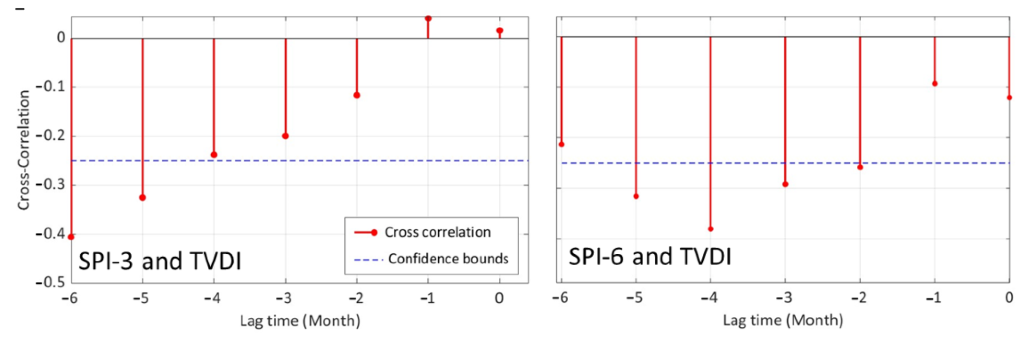
For determining the maximum i and j, the cross-correlation function RTVDI, SPI between two time series is defined by following Equation (21), i.e., the discrete cross correlation between TVDI and SPIm (m = 3, m = 6) with N data at the lag time l, which reads as [48]:
The cross-correlation functions between both drought indices have been calculated to see the lag-time between SPI with different time scales and TVDI. Figure 8 shows that the is mostly correlated with . Therefore, the final input-output Wavelet-ANFIS model Equation (19) can be written as:
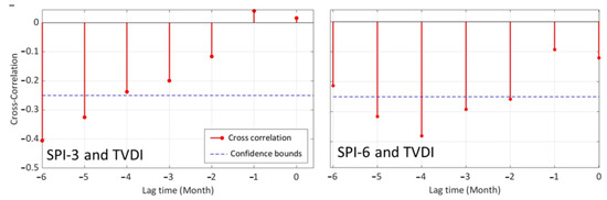
Figure 8.
Cross correlation function between meteorological and agricultural drought indices, namely standard precipitation index (SPI) and temperature vegetation dryness index (TVDI).left panel: SPI3-month and TVDI; right panel: SPI6-month and TVDI.
To conduct model training and testing, the 52 TVDI values were distributed across 36 months. When there were two satellite overpasses in a given month, the average of those values was used as the month’s representative TVDI. Additionally, 8 extreme data points (with TVDI values of 0.2 and 0.9, corresponding to SPI values of 2.9 and −2.9, representing extremely wet and dry conditions) were introduced artificially to ensure that all data fell within the specified range [0, 1]. In order to augment the TVDI dataset, a specific TVDI value (denoted as ) have been assigned to each corresponding SPI input (, where i ranges from 2 to 6). This resulted in 191 TVDI data points for 191 SPI inputs (199 considering 8 extreme values). Furthermore, for each of these data points, a random value within the range [0, 1] was generated and multiplied by ±0.05. These random values, falling within the interval [−0.05, 0.05], were then added to the original TVDI values. This augmentation process increased the dataset size to a total of 597 data points.
The proposed scientific methodology comprises of three distinct components: discrete wavelet transform/multiresolution analysis (DWT/MRA), fuzzy C-means (FCM) clustering and ANFIS [31]. These techniques will be elaborated in subsequent sections.
2.7.1. Multiresolution Analysis of Input Data Using the Discrete Wavelet Transform
The analysis of a time series using wavelets is an expansion of traditional Fourier analysis. Unlike Fourier analysis, wavelet analysis enables the identification of the frequency content of a time signal at a specific time point, even if the signal is non-stationary. In practical applications, two main forms of wavelet analysis are distinguished: the continuous wavelet transform (CWT), which is used to generate two-dimensional time-frequency (or scale) scalograms of a time-series, and the discrete wavelet transform (DWT), which is used primarily to approximate high-frequency signals at lower frequency levels by performing a low-pass (resolution) filtering, see [31] for more details. The DWT of a time series of x(t) is defined as [49,50] and was chosen here:
where aj = 2j is the scale (i.e., inverse of frequency) (dilatated/compressed), bk = k 2j is the shift (translate) parameter, and is the wavelet, i.e., are the scaled and shifted wavelets. If the wavelet function belongs to a so-called tight frame of wavelet classes, forms a complete and orthonormal basis, so that the signal x(t) can be reconstructed by the classical formula
This equation is the basis of the MRA [51] Using the fundamental decomposition exposed by Equation (23) over the finite range of scales and shift times, one obtains the equation for the complete decomposition of the signal x(t). The wavelet function can cover the whole frequency range of the signal, starting from the Nyquist sampling frequency (the lowest scale) down to a minimum frequency (highest scale). High scale (low frequency) component of x(t), generated by the low-pass scaling function. It represents the Aj max-approximation of the signal at the highest decomposition level. The low-scale, high frequency details Dj of the signal, generated by the high-pass wavelet functions (j = 1,.., jmax). Thus, Equation (24) can be simplified as [23,25,51]:
When it comes to selecting the discrete scaling and wavelet filter functions for DWT/MRA, the popular choices include Haar, Daubechies wavelet (db), and Symlet (sym) irregular wavelet. Haar is the most basic mother wavelet function that is orthogonal. However, it may not be able to capture nonlinear shifts between input and decomposed signals because it only has two filtering taps and a linear phase. In contrast, db and Sym mother wavelets have 2N filtering taps and are better suited for applications where capturing nonlinear shifts is necessary. In this study, the sym irregular wavelet with order 4 was the most appropriate option (Figure 9).
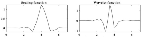
Figure 9.
Scaling and wavelet function for the sym4 wavelet.
2.7.2. Fuzzy C-Means (FCM) Clustering
After applying MRA to decompose the input signals, and the resulting approximations are included into the fuzzy C-means (FCM) clustering module. FCM is a modified and enhanced version of K-means clustering, in which every data point belongs partially to each cluster with a varying membership degree between 0 and 1.
2.7.3. Hybrid Wavelet-ANFIS/FCM Model
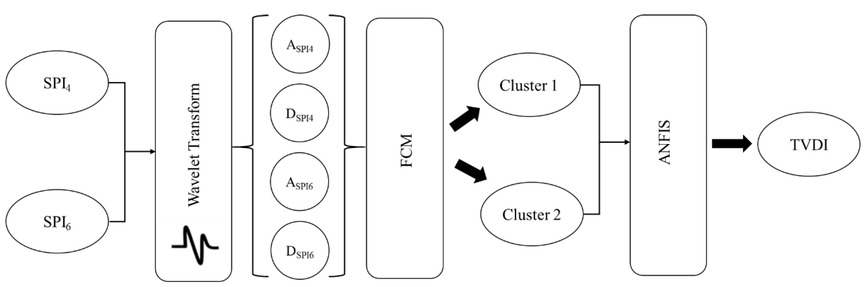
The ANFIS model is the last step in the machine learning methodology. The ANFIS class of adaptive neural networks is functionally equivalent to fuzzy inference systems. As introduced by [26], ANFIS is a network-based model that combines fuzzy logic and artificial neural networks (network-based architecture) By putting all pieces together, the flowchart of the whole hybrid Wavelet-ANFIS/FCM model developed by [26] is obtained (Figure 10).
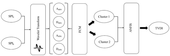
Figure 10.
Flowchart of the hybrid Wavelet-ANFIS/FCM model.
3. Results and Discussions
3.1. Meteorological and Agricultural Drought Index
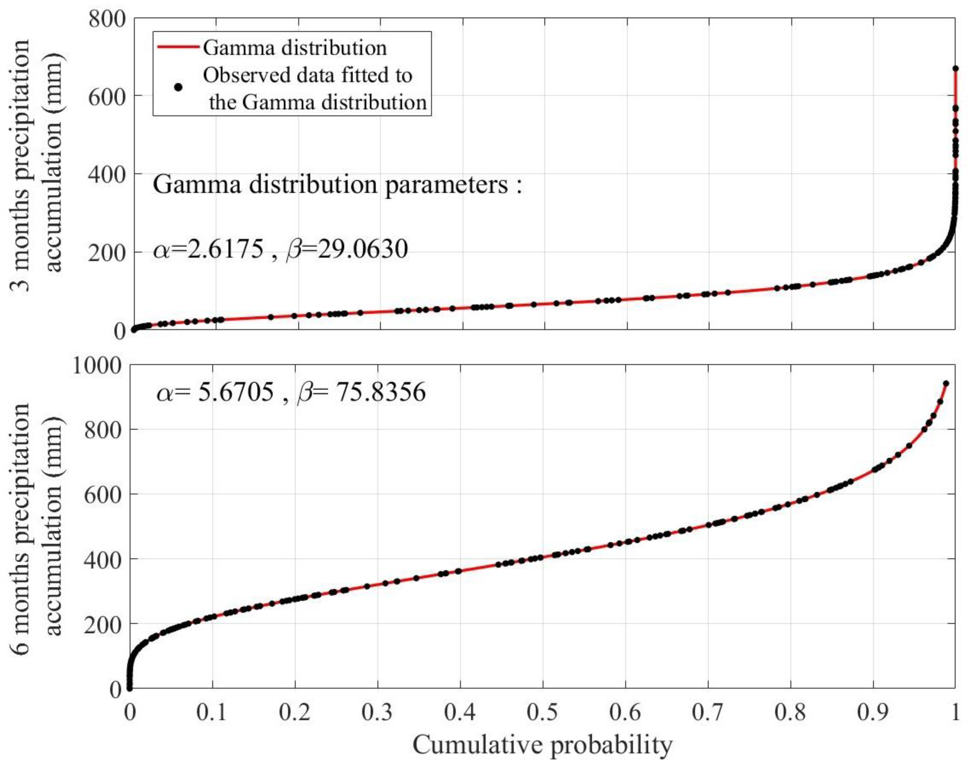
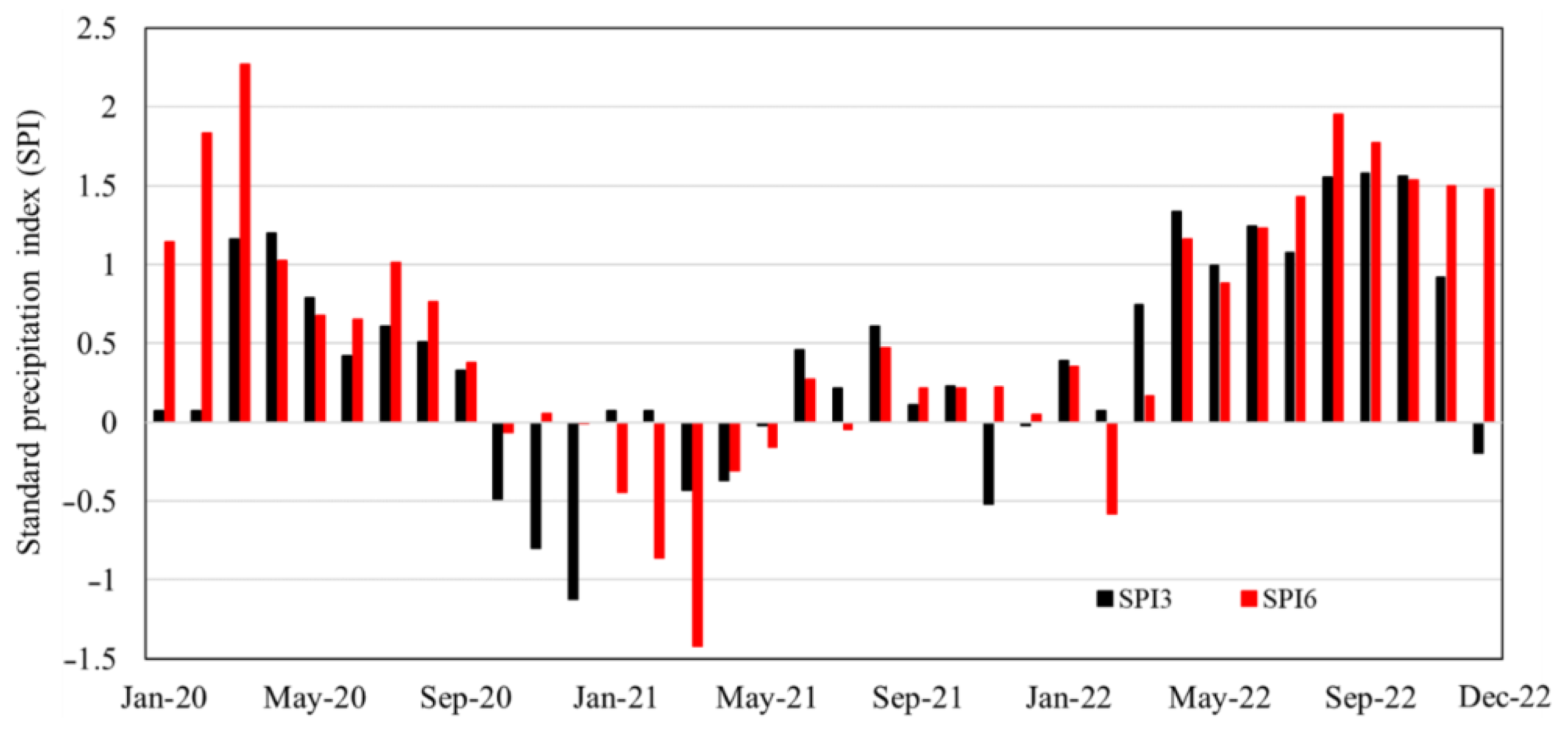
The SPI have been calculated for 3 and 6-months time scales, using the gamma distribution parametric method (Figure 11) for the long-term time series of observed monthly precipitation (2005–2022) in Tamale, Ghana. In Figure 12, the SPI values for the period 2020–2022 extracted from the gamma distribution are shown. For the first half of 2020, higher than normal rainfall conditions with maxima in March and April can be stated. Then the SPI values decline and it becomes dryer than normal for the first half of 2021. With beginning of 2022, SPI values strongly increase again showing higher than usual wet conditions for August until October for this year.
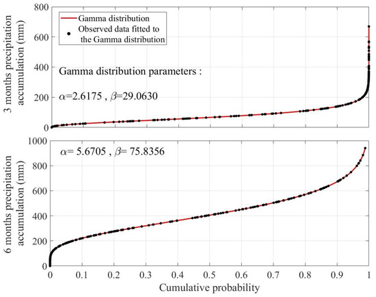
Figure 11.
Fitted Gamma distribution on observed monthly precipitation accumulation (mm) for calculating SPI3 (top panel) and SPI6 (bottom panel).

Figure 12.
The SPI values for three consecutive years (2020–2022).
For the same time interval, all agricultural drought events were calculated using the TVDI values delineated from satellite data (Landsat 8 and 9). The TVDI is based on LST-NDVI (Land surface temperature-normalized difference vegetation index) using the trapezoidal area and split window method, for more details please see. [9]. Using the equation of dry and wet edges of trapezoidal space, the TVDI was estimated for each pixel of Landsat 8/9 satellite images. Figure 13 shows the procedure of TVDI calculation for Landsat 9 satellite image (path/row: 194/53) on 6 November 2022.
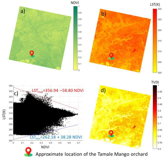
Figure 13.
(a) The spatial distribution of normalized difference vegetation index (NDVI), (b) land surface temperature (LST) using the split window (SW) method, (c) the Trapezoidal space of LST/NDVI, and (d) the Temperature Vegetation Dryness Index (TVDI) based on Landsat 9 satellite images (path/row: 194/53) acquired on 6th November 2022. The wet edge is represented by the blue line (TVDI = 0), while the dry edge is marked by the red line (TVDI = 1).
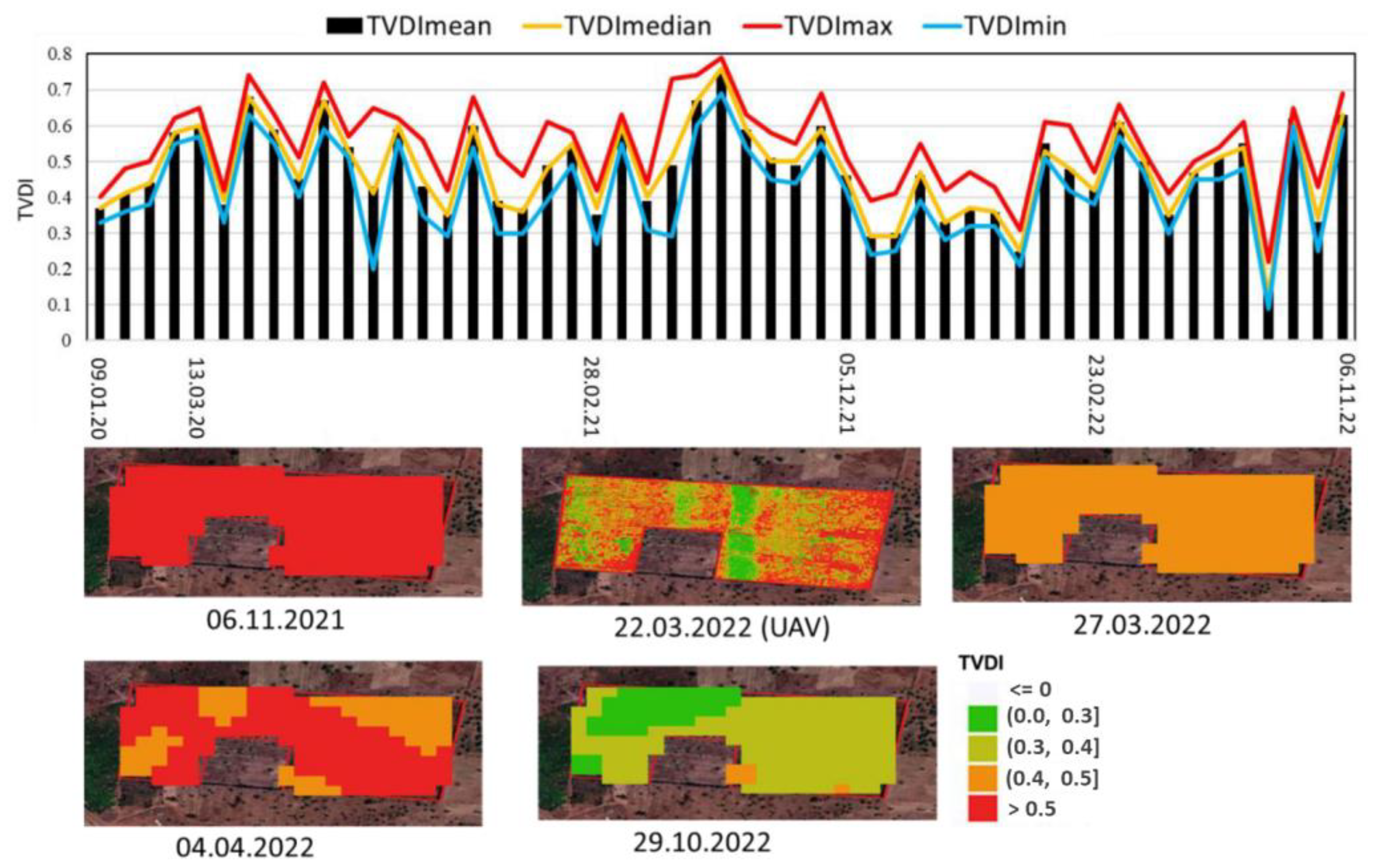
The TVDI for the Tamale Mango orchard was determined by isolating the specific study area from all satellite-based TVDI maps listed in Table 2 (refer to Figure 14 for details). The average TVDI value has been utilized as an indicator to assess agricultural drought conditions within the orchard. In order to validate the accuracy of the satellite-based TVDI maps, the resolution of the satellite data recorded on 27 March 2022, has been adjusted to match the resolution of the UAV ortho image obtained on 22 March 2022, and the results were subsequently compared for consistency. As Figure 15 shows, within the dataset, 74% (133 out of 180) of the pixels exhibit an absolute error of less than 0.1 when comparing two similar pixels from the TVDI maps, while 93% of the pixels have an absolute error of less than 0.2.

Figure 14.
(Upper panel) statistical evaluation of Temperature Vegetation Dryness Index (TVDI) maps across 51 Landsat 8/9 images; (Lower panel) the spatial distribution of TVDI in four satellite overpasses and one UAV (Unmanned Aerial Vehicle) image.
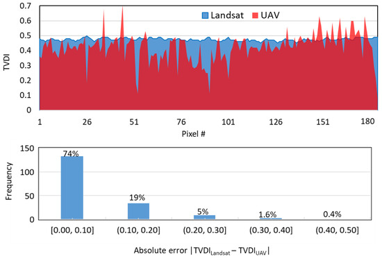
Figure 15.
Analysis of Absolute Error in Temperature Vegetation Dryness Index (TVDI) maps derived from Landsat and UAV based data.
3.2. Climate Change Scenarios
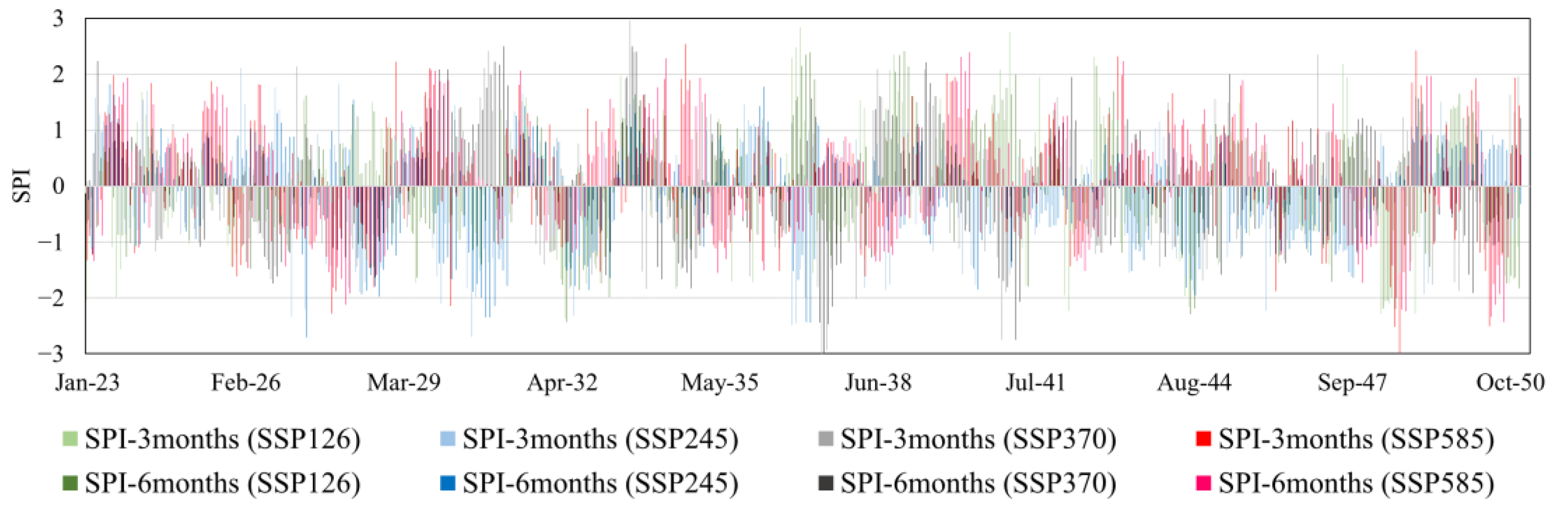
In order to project the standard precipitation index (SPI) values for the period spanning from 2023 to 2050, the SPI 3 and 6-month values were extrapolated based on projected rainfall data obtained from the four Shared Socioeconomic Pathways (SSPs)—namely, SSP126, SSP245, SSP370, and SSP585. The analyses were conducted within the framework of CMIP6 (Coupled Model Intercomparison Project Phase 6), which has been utilized to provide a comprehensive basis for climate model comparison and projection. Across all 35 models for each SSP scenario, the median values of monthly precipitation were used to calculate the SPI 3 and 6-month values. Figure 16 shows an overview of the SPI patterns and variations associated with these different scenarios.
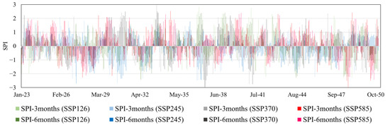
Figure 16.
The standard precipitation index (SPI) with time scale of 3 and 6 months using 4 different Shared Socioeconomic Pathways (SSPs) within the framework of CMIP6 (Coupled Model Intercomparison Project Phase 6).
Using Equation (22) (), the agricultural drought based on the TVDI was predicted using the Hybrid Wavelet-ANFIS/FCM model from 2023 to 2050.
3.3. Wavelet ANFIS Model Results
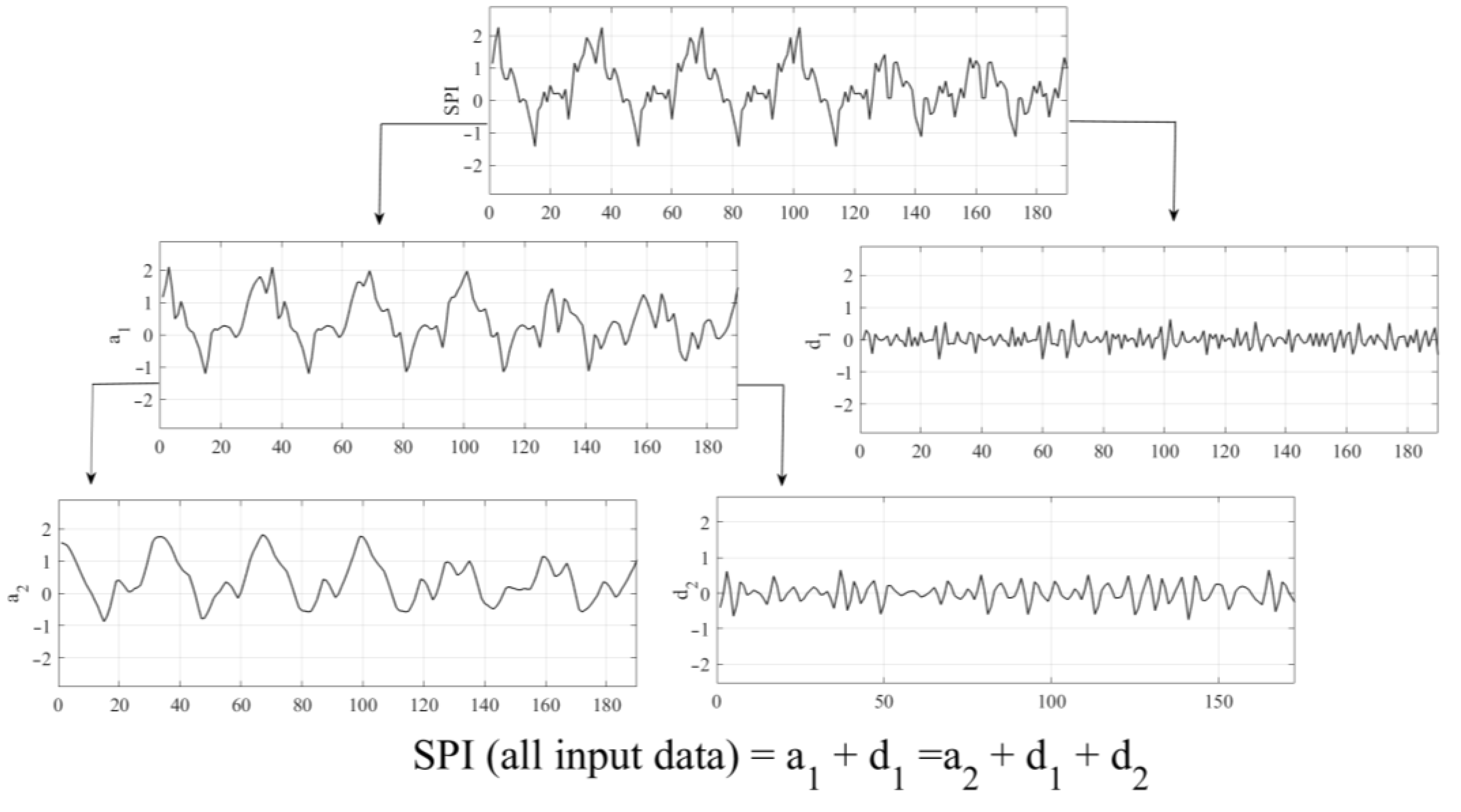
By employing the sym4 wavelet for Multiresolution Analysis (MRA) on all SPI values within Equation (22) and subsequently applying Equations (24) and (25), we have successfully obtained the 2-level multiresolution decompositions of the monthly data time series spanning three years (2020–2022), as depicted in Figure 17.
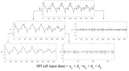
Figure 17.
2-level MRA-decomposition of standard precipitation index (SPI) using the sym4 wavelet.
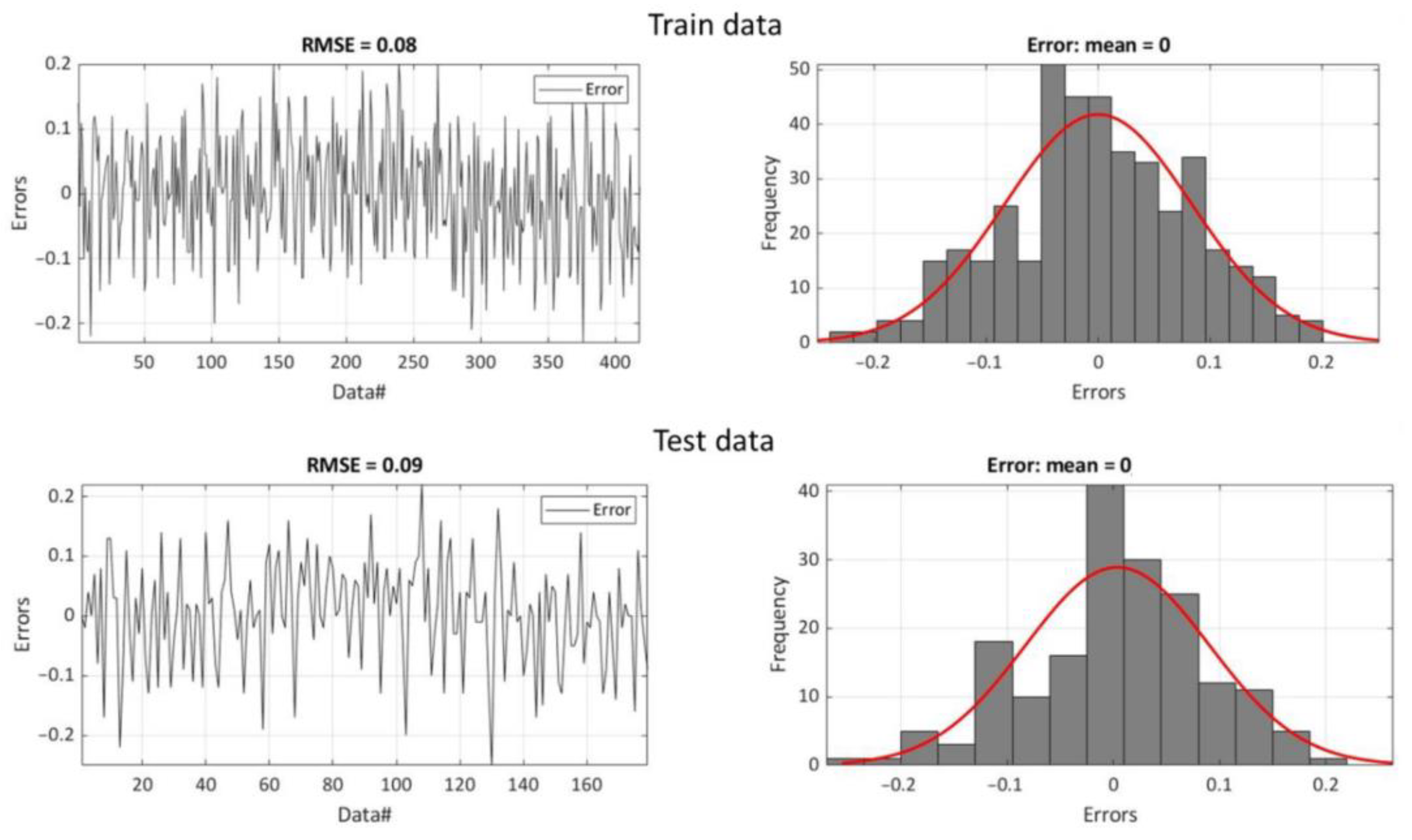
Using the algorithm of the hybrid wavelet-ANFIS/FCM-model as sketched in Figure 10, TVDI-fluctuations were simulated first. The results are shown in Figure 18 for the training and testing phases of the data period and they indicate that the simulated TVDIs match the observed ones rather well with a root mean square errors, RMSE, of less than 0.1 in both training and testing phases. More details of the statistical results of the hybrid Wavelet-ANFIS/FCM model are illustrated by errors plots of the simulated over the observed TVDI-data in the left panel of Figure 19, which clearly indicate that the selected hybrid model delivers good and reliable predictions of the TVDI. All data-driven prediction methods are based on the idea that the random errors are drawn from a normal distribution and the hybrid Wavelet-ANFIS model is not an exemption. The histograms of Figure 19 illustrates that a posteriori computed errors of the computed TVDIs with this model follow indeed a normal distribution.
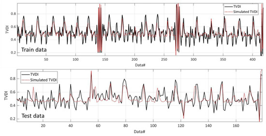
Figure 18.
Wavelet-ANFIS/Sym4—simulated and observed TVDI for the training (upper panel) and testing (lower panel) phases.
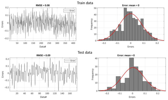
Figure 19.
Distribution of the TVDI-random errors of the wavelet-ANFIS model.
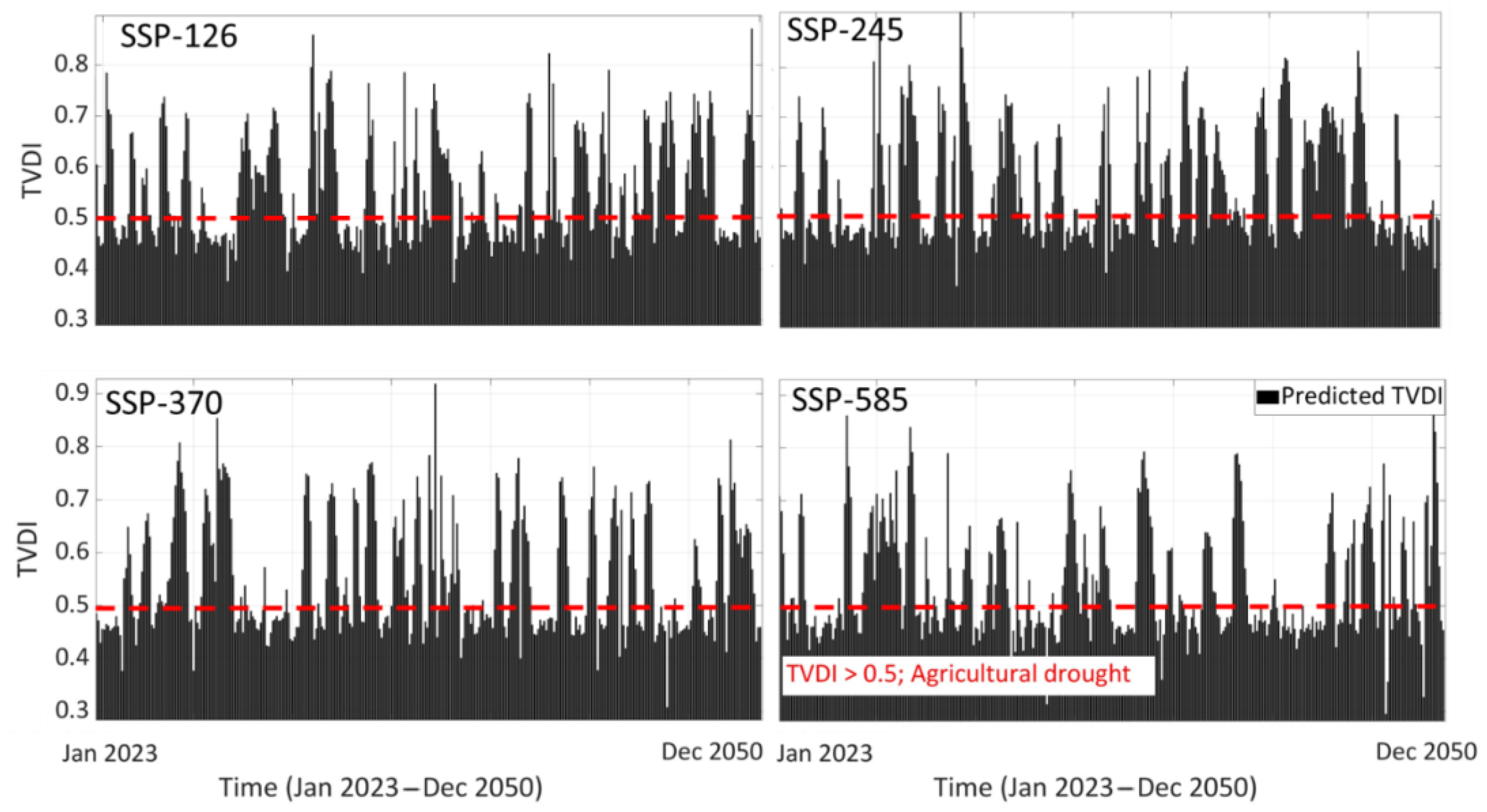
Figure 20 shows the monthly TVDI predictions calculated from utilizing Equation (22) with the hybrid wavelet-ANFIS model for the Mango orchard located in Tamale for the time period of 2023 to 2050. These predictions were based on input values derived from the SPI modeled by using various climate change scenarios under the Shared Socioeconomic Pathways (SSPs). It can be used as an agricultural drought indicator, where TVDI values exceeding 0.5 serve as an indicator of orchard water stress.
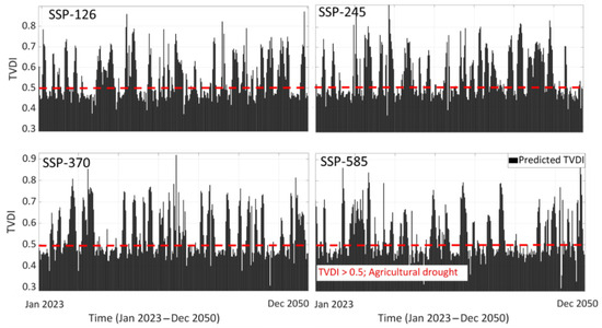
Figure 20.
TVDI predictions for the period of 2023–2050 under the Shared Socioeconomic Pathways (SSPs) climate change scenarios.
An examination of the outcomes depicted in Figure 20 reveals that, across the SSP126, SSP245, SSP370, and SSP585 scenarios, 186, 183, 179, and 179 months are estimated to exceed TVDI levels of 0.5. Within the timeframe, spanning from 2023 to 2050, this orchard is expected to experience agricultural drought conditions depending on climate change. This implies that over 50% of the time, under all climate change scenarios, the area will grapple with such conditions. These findings highlight the pronounced prevalence of water stress in the Tamale mango orchard, underscoring the imperative need for the implementation of supplementary irrigation systems to mitigate the adverse consequences of agricultural drought, particularly in light of the evolving climate conditions.
In this study, the agricultural drought index, the TVDI, has been modelled using the meteorological drought index, the SPI. Drawing upon climate models outlined by the IPCC, frequency of drought conditions in a mango orchard located in Tamale, Ghana, has been projected for the forthcoming decades. Aligning with results of present study, Bedair et al. [14] underscore the heightened vulnerability of Ghana to drought. This heightened risk jeopardizes food security and poses threats to both human and livestock well-being. While current models relying on the SPI have provided acceptable short-term predictions for drought conditions [7], the results this research emphasis on a comprehensive, long-term projection. It has been indicated that the region will be significantly (more than 50% of the projected months) affected by agricultural drought conditions across all types of SSP climate change scenarios.
4. Conclusions
The research findings unveiled a comprehensive understanding of the relationship between the meteorological and agricultural drought indices, namely, SPI and TVDI. They were subsequently integrated into the Wavelet-ANFIS predictive model, which was employed to estimate TVDI as an agricultural drought indicator for the extensive period spanning from 2023 to 2050.
The results revealed that significant water stress will be observed in the Tamale mango orchard under diverse climate change scenarios represented by the Shared Socioeconomic Pathways (SSPs). A high number of months, specifically, 186, 183, 179, and 179 months for SSP126, SSP245, SSP370, and SSP585, respectively, was characterized by agricultural drought conditions for this forthcoming period. That corresponds to 55–57% of the projected months. These findings underscored the pressing need for proactive measures like supplementary irrigation to safeguard the orchard’s agricultural sustainability in the next decades. According to [52], models can be used to support decision making for long-term transformative responses that require strategic planning. Such measures are pivotal in ensuring the resilience of agricultural activities in the face of climate change and thus guarantee local food security.
In conclusion, this research was a critical step towards unraveling the complex dynamics of meteorological drought and its profound implications for agriculture. The Wavelet-ANFIS predictive model exposed imminent challenges faced by the Tamale mango orchard, which can point the way to a more resilient and sustainable agricultural future. Acknowledging these challenges and implementing decisive measures, e.g., supplementary irrigation systems or crop adaptations, holds the key to ensure economic stability in the midst of ongoing climate change. To enhance our understanding of agricultural drought dynamics and adaptation strategies, future research should focus on improving data-driven predictive models by integrating additional spatial and temporal data sources. This entails considering climate model uncertainty, evaluating socioeconomic impacts, establishing long-term monitoring programs, and expanding research to other geographic regions with varying climate conditions.
Author Contributions
Conceptualization, M.Z. and M.H.; methodology, M.Z and S.K.; software, M.Z. and M.H. validation, M.Z., M.S. and M.H.; formal analysis, M.Z.; investigation, M.Z., M.H., G.B.-M., A.-H.A. and M.S.; resources, M.Z., M.H., A.-H.A. and M.S.; data curation, M.Z., M.H. and M.S.; writing—original draft preparation, M.Z.; writing—review and editing, M.Z.; M.S., M.H., G.B.-M., A.-H.A. and S.K. visualization, M.Z., M.H. and M.S.; supervision, M.S.; project administration, M.S.; funding acquisition, M.S., A.-H.A. and G.B.-M. All authors have read and agreed to the published version of the manuscript.
Funding
This article was co-funded from the European Union’s Horizon 2020 Research and Innovation Programme under grand agreement No. 861924.
Data Availability Statement
Data and used scripts for this paper can be downloaded at https://github.com/hyddata (accessed on 21 March 2024).
Conflicts of Interest
Author Godwin Badu-Marfo was employed by the company Dexafrica Limited. The remaining authors declare that the research was conducted in the absence of any commercial or financial relationships that could be construed as a potential conflict of interest.
References
- IPCC. Climate Change 2022: Impacts, Adaptation, and Vulnerability. Contribution of Working Group II to the Sixth Assessment Report of the Intergovernmental Panel on Climate Change; Pörtner, H.-O., Roberts, D.C., Tignor, M., Poloczanska, E.S., Mintenbeck, K., Alegría, A., Craig, M., Langsdorf, S., Löschke, S., Möller, V., et al., Eds.; Cambridge University Press: Cambridge, UK; New York, NY, USA, 2022; 3056p. [Google Scholar] [CrossRef]
- Zare, M.; Schumann, G.J.-P.; Teferle, F.N.; Mansorian, R. Generating Flood Hazard Maps Based on an Innovative Spatial Interpolation Methodology for Precipitation. Atmosphere 2021, 12, 1336. [Google Scholar] [CrossRef]
- Pascoe, C.; Lawrence, B.N.; Guilyardi, E.; Juckes, M.; Taylor, K.E. Documenting Numerical Experiments in Support of the Coupled Model Intercomparison Project Phase 6 (CMIP6). Geosci. Model Dev. 2020, 13, 2149–2167. [Google Scholar] [CrossRef]
- Riahi, K.; van Vuuren, D.P.; Kriegler, E.; Edmonds, J.; O’Neill, B.C.; Fujimori, S.; Bauer, N.; Calvin, K.; Dellink, R.; Fricko, O.; et al. The Shared Socioeconomic Pathways and Their Energy, Land Use, and Greenhouse Gas Emissions Implications: An Overview. Glob. Environ. Change 2017, 42, 153–168. [Google Scholar] [CrossRef]
- Ding, Y.; Gong, X.; Xing, Z.; Cai, H.; Zhou, Z.; Zhang, D.; Sun, P.; Shi, H. Attribution of Meteorological, Hydrological and Agricultural Drought Propagation in Different Climatic Regions of China. Agric. Water Manag. 2021, 255, 106996. [Google Scholar] [CrossRef]
- Van Loon, A.F.; Laaha, G. Hydrological Drought Severity Explained by Climate and Catchment Characteristics. J. Hydrol. 2015, 526, 3–14. [Google Scholar] [CrossRef]
- Paxian, A.; Ziese, M.; Kreienkamp, F.; Pankatz, K.; Brand, S.; Pasternack, A.; Früh, B. User-oriented global predictions of the GPCC drought index for the next decade. Meteorol. Z. 2019, 28, 3–21. [Google Scholar] [CrossRef]
- Wilhite, D.A.; Sivakumar, M.V.K.; Pulwarty, R. Managing Drought Risk in a Changing Climate: The Role of National Drought Policy. Weather Clim. Extrem. 2014, 3, 4–13. [Google Scholar] [CrossRef]
- Zare, M.; Drastig, K.; Zude-Sasse, M. Tree Water Status in Apple Orchards Measured by Means of Land Surface Temperature and Vegetation Index (LST–NDVI) Trapezoidal Space Derived from Landsat 8 Satellite Images. Sustainability 2020, 12, 70. [Google Scholar] [CrossRef]
- Sun, D.; Pinker, R.T. Estimation of Land Surface Temperature from a Geostationary Operational Environmental Satellite (GOES-8). J. Geophys. Res. Atmos. 2003, 108. [Google Scholar] [CrossRef]
- Sheng, J.; Wilson, J.P.; Lee, S. Comparison of Land Surface Temperature (LST) Modeled with a Spatially-Distributed Solar Radiation Model (SRAD) and Remote Sensing Data. Environ. Model. Softw. 2009, 24, 436–443. [Google Scholar] [CrossRef]
- Yang, J.; Wang, Y. Estimating Evapotranspiration Fraction by Modeling Two-Dimensional Space of NDVI/Albedo and Day–Night Land Surface Temperature Difference: A Comparative Study. Adv. Water Resour. 2011, 34, 512–518. [Google Scholar] [CrossRef]
- Zare, M.; Drastig, K.; Zude-Sasse, M. Estimating Tree Water Status in Apple Orchard Using Reflectance in the Thermal Domain of Landsat 8 Satellite. In Proceedings of the 2019 IEEE International Workshop on Metrology for Agriculture and Forestry (MetroAgriFor), Portici, Italy, 24–26 October 2019; pp. 255–259. [Google Scholar] [CrossRef]
- Bedair, H.; Alghariani, M.S.; Omar, E.; Anibaba, Q.A.; Remon, M.; Bornman, C.; Alzain, H.M. Global Warming Status in the African Continent: Sources, Challenges, Policies, and Future Direction. Int. J. Environ. Res. 2023, 17, 45. [Google Scholar] [CrossRef]
- Yi, Q.; Bao, A.; Wang, Q.; Zhao, J. Estimation of Leaf Water Content in Cotton by Means of Hyperspectral Indices. Comput. Electron. Agric. 2013, 90, 144–151. [Google Scholar] [CrossRef]
- Guermazi, E.; Bouaziz, M.; Zairi, M. Water Irrigation Management Using Remote Sensing Techniques: A Case Study in Central Tunisia. Environ. Earth Sci. 2016, 75, 202. [Google Scholar] [CrossRef]
- Ozelkan, E.; Chen, G.; Ustundag, B.B. Multiscale Object-Based Drought Monitoring and Comparison in Rainfed and Irrigated Agriculture from Landsat 8 OLI Imagery. Int. J. Appl. Earth Obs. Geoinf. 2016, 44, 159–170. [Google Scholar] [CrossRef]
- Veysi, S.; Naseri, A.A.; Hamzeh, S.; Bartholomeus, H. A Satellite Based Crop Water Stress Index for Irrigation Scheduling in Sugarcane Fields. Agric. Water Manag. 2017, 189, 70–86. [Google Scholar] [CrossRef]
- Nugraha, A.S.A.; Gunawan, T.; Kamal, M. Modification of Temperature Vegetation Dryness Index (TVDI) Method for Detecting Drought with Multi-Scale Image. IOP Conf. Ser. Earth Environ. Sci. 2022, 1039, 012048. [Google Scholar] [CrossRef]
- Brion, G.M.; Neelakantan, T.R.; Lingireddy, S. A Neural-Network-Based Classification Scheme for Sorting Sources and Ages of Fecal Contamination in Water. Water Res. 2002, 36, 3765–3774. [Google Scholar] [CrossRef] [PubMed]
- Goel, A.; Goel, A.K.; Kumar, A. The Role of Artificial Neural Network and Machine Learning in Utilizing Spatial Information. Spat. Inf. Res. 2023, 31, 275–285. [Google Scholar] [CrossRef]
- Nayak, P.C.; Sudheer, K.P.; Rangan, D.M.; Ramasastri, K.S. A Neuro-Fuzzy Computing Technique for Modeling Hydrological Time Series. J. Hydrol. 2004, 291, 52–66. [Google Scholar] [CrossRef]
- Zare, M.; Koch, M. Hybrid Signal Processing/Machine Learning and PSO Optimization Model for Conjunctive Management of Surface–Groundwater Resources. Neural Comput. Appl. 2021, 33, 8067–8088. [Google Scholar] [CrossRef]
- Jang, J.-S. ANFIS: Adaptive-network-based fuzzy inference system. IEEE Trans. Syst. Man Cybern. 1993, 23, 665–685. [Google Scholar] [CrossRef]
- Jang, J.-S.; Sun, C.-T. Neuro-Fuzzy Modeling and Control. Proc. IEEE 1995, 83, 378–406. [Google Scholar] [CrossRef]
- Zare, M. Application and Analysis of Physical and Data-Driven Stochastic Hydrological Simulation-Optimization Methods for the Optimal Management of Surface-Groundwater Resources Systems; University of Kassel: Kassel, Germany, 2017. [Google Scholar]
- Dikshit, A.; Pradhan, B.; Santosh, M. Artificial Neural Networks in Drought Prediction in the 21st Century—A Scientometric Analysis. Appl. Soft Comput. 2022, 114, 108080. [Google Scholar] [CrossRef]
- Mohammed, S.; Elbeltagi, A.; Bashir, B.; Alsafadi, K.; Alsilibe, F.; Alsalman, A.; Zeraatpisheh, M.; Széles, A.; Harsányi, E. A Comparative Analysis of Data Mining Techniques for Agricultural and Hydrological Drought Prediction in the Eastern Mediterranean. Comput. Electron. Agric. 2022, 197, 106925. [Google Scholar] [CrossRef]
- Prodhan, F.A.; Zhang, J.; Hasan, S.S.; Pangali Sharma, T.P.; Mohana, H.P. A Review of Machine Learning Methods for Drought Hazard Monitoring and Forecasting: Current Research Trends, Challenges, and Future Research Directions. Environ. Model. Softw. 2022, 149, 105327. [Google Scholar] [CrossRef]
- Adnan, R.M.; Dai, H.-L.; Kuriqi, A.; Kisi, O.; Zounemat-Kermani, M. Improving Drought Modeling Based on New Heuristic Machine Learning Methods. Ain Shams Eng. J. 2023, 14, 102168. [Google Scholar] [CrossRef]
- Zare, M.; Koch, M. Groundwater Level Fluctuations Simulation and Prediction by ANFIS- and Hybrid Wavelet-ANFIS/Fuzzy C-Means (FCM) Clustering Models: Application to the Miandarband Plain. J. Hydro-Environ. Res. 2018, 18, 63–76. [Google Scholar] [CrossRef]
- Petrie, R.; Denvil, S.; Ames, S.; Levavasseur, G.; Fiore, S.; Allen, C.; Antonio, F.; Berger, K.; Bretonnière, P.-A.; Cinquini, L.; et al. Coordinating an Operational Data Distribution Network for CMIP6 Data. Geosci. Model Dev. 2021, 14, 629–644. [Google Scholar] [CrossRef]
- Zare, M. Download CMIP6 Data. Available online: https://Github.Com/Hyddata/CMIP6_data (accessed on 21 March 2024).
- Giustarini, L.; Schumann, G.J.-P.; Kettner, A.J.; Smith, A.; Nawrotzki, R. Simulating Changes in Hydrological Extremes—Future Scenarios for Morocco. Water 2023, 15, 2722. [Google Scholar] [CrossRef]
- USGS. Landsat 8 Data Users Handbook; USGS: Sioux Falls, SD, USA, 2016. [Google Scholar]
- USGS. Landsat 9 Data Users Handbook; USGS: Sioux Falls, SD, USA, 2022. [Google Scholar]
- Tucker, C.J. Red and Photographic Infrared Linear Combinations for Monitoring Vegetation. Remote Sens. Environ. 1979, 8, 127–150. [Google Scholar] [CrossRef]
- Mao, K.; Qin, Z.; Shi, J.; Gong, P. A Practical Split-window Algorithm for Retrieving Land-surface Temperature from MODIS Data. Int. J. Remote Sens. 2005, 26, 3181–3204. [Google Scholar] [CrossRef]
- Rozenstein, O.; Qin, Z.; Derimian, Y.; Karnieli, A. Correction: Rozenstein, O.; et al. Derivation of Land Surface Temperature for Landsat-8 TIRS Using a Split Window Algorithm. Sensors 2014, 14, 11277. [Google Scholar] [CrossRef]
- Qin, Z.; Dall’Olmo, G.; Karnieli, A.; Berliner, P. Derivation of Split Window Algorithm and Its Sensitivity Analysis for Retrieving Land Surface Temperature from NOAA-Advanced Very High Resolution Radiometer Data. J. Geophys. Res. Atmos. 2001, 106, 22655–22670. [Google Scholar] [CrossRef]
- Yang, L.; Cao, Y.; Zhu, X.; Zeng, S.; Yang, G.; He, J.; Yang, X. Land Surface Temperature Retrieval for Arid Regions Based on Landsat-8 TIRS Data: A Case Study in Shihezi, Northwest China. J. Arid Land 2014, 6, 704–716. [Google Scholar] [CrossRef]
- Sobrino, J.A.; Jiménez-Muñoz, J.C.; Paolini, L. Land Surface Temperature Retrieval from LANDSAT TM 5. Remote Sens. Environ. 2004, 90, 434–440. [Google Scholar] [CrossRef]
- Nikam, B.R.; Ibragimov, F.; Chouksey, A.; Garg, V.; Aggarwal, S.P. Retrieval of Land Surface Temperature from Landsat 8 TIRS for the Command Area of Mula Irrigation Project. Environ. Earth Sci. 2016, 75, 1169. [Google Scholar] [CrossRef]
- Abuzar, M.; O’Leary, G.; Fitzgerald, G. Measuring Water Stress in a Wheat Crop on a Spatial Scale Using Airborne Thermal and Multispectral Imagery. Field Crops Res. 2009, 112, 55–65. [Google Scholar] [CrossRef]
- Zhang, F.; Zhang, L.-W.; Shi, J.-J.; Huang, J.-F. Soil Moisture Monitoring Based on Land Surface Temperature-Vegetation Index Space Derived from MODIS Data. Pedosphere 2014, 24, 450–460. [Google Scholar] [CrossRef]
- Mckee, T.B.; Doesken, N.J.; Kleist, J.R. The Relationship of Drought Frequency and Duration to Time Scales. In Proceedings of the 8th Conference on Applied Climatology, Anaheim, CA, USA, 17–22 January 1993; pp. 179–184. [Google Scholar]
- Mansorian, R.; Zare, M.; Schumann, G. Study on the Correlation between Meteorological and Agricultural Drought, Based on Remotely Sensed Indices. In Proceedings of the EGU General Assembly Conference Abstracts, Vienna, Austria, 4–8 May 2020; p. 13925. [Google Scholar] [CrossRef]
- Fathian, F. Chapter 3—Introduction of Multiple/Multivariate Linear and Nonlinear Time Series Models in Forecasting Streamflow Process. In Advances in Streamflow Forecasting; Sharma, P., Machiwal, D., Eds.; Elsevier: Amsterdam, The Netherlands, 2021; pp. 87–113. ISBN 978-0-12-820673-7. [Google Scholar]
- Jukić, D.; Denić-Jukić, V.; Kadić, A. Temporal and Spatial Characterization of Sediment Transport through a Karst Aquifer by Means of Time Series Analysis. J. Hydrol. 2022, 609, 127753. [Google Scholar] [CrossRef]
- Mallat, S.G. A Theory for Multiresolution Signal Decomposition: The Wavelet Representation. IEEE Trans. Pattern Anal. Mach. Intell. 1989, 11, 674–693. [Google Scholar] [CrossRef]
- Kim, J.; Chun, C.-Y. Cho Implementation of EKF Combined with Discrete Wavelet Transform-Based MRA for Improved SOC Estimation for a Li-Ion Cell. In Proceedings of the 2013 Twenty-Eighth Annual IEEE Applied Power Electronics Conference and Exposition (APEC), Long Beach, CA, USA, 17–21 March 2013; pp. 2720–2725. [Google Scholar] [CrossRef]
- Holzkämper, A. Adapting Agricultural Production Systems to Climate Change—What’s the Use of Models? Agriculture 2017, 7, 86. [Google Scholar] [CrossRef]


Disclaimer/Publisher’s Note: The statements, opinions and data contained in all publications are solely those of the individual author(s) and contributor(s) and not of MDPI and/or the editor(s). MDPI and/or the editor(s) disclaim responsibility for any injury to people or property resulting from any ideas, methods, instructions or products referred to in the content. |
© 2024 by the authors. Licensee MDPI, Basel, Switzerland. This article is an open access article distributed under the terms and conditions of the Creative Commons Attribution (CC BY) license (https://creativecommons.org/licenses/by/4.0/).