Monitoring Land Use Changes in the Yellow River Delta Using Multi-Temporal Remote Sensing Data and Machine Learning from 2000 to 2020

Abstract

The Yellow River Delta (YRD), known for its vast and diverse wetland ecosystem, is the largest estuarine delta in China. However, human activities and climate change have significantly degraded the wetland ecosystem in recent decades in the YRD. Therefore, an understanding of the land use modifications is essential for the efficient management and preservation of ecosystems in this region. This study utilized time series of remote sensing data and the extreme gradient boosting method to generate land use maps of the YRD from 2000 to 2020. Several methods, including transition matrix, land use dynamic degree, and standard deviation ellipse, were employed to explore the characteristics of land use transitions. The results underscore significant spatial variations in land use over the past two decades. The most rapid increase was observed in built-up area, followed by terrestrial water and tidal flats, while unutilized land experienced the fastest decrease, followed by forest–grassland. The spatial distribution patterns of agricultural land, built-up area, terrestrial water, and forest–grassland demonstrated stronger directionality compared to other land use types. The wetlands have expanded in size and improved in structure. Unutilized land has been converted into artificial wetlands comprising ponds, reservoirs, salt ponds, shrimp and crab ponds, and natural wetlands featuring mudflats and forest–grassland. The wetland conservation efforts after 2008 have proven very effective, playing a positive role in ecological and environmental preservation, as well as in regional sustainable development.

1. Introduction

Land use/cover transformation serves as an important indicator of the impacts of human activities on the Earth’s surface and is an essential aspect of global environmental change [1]. With the progress of global urbanization, land cover and land use have changed significantly, causing various problems, including biodiversity loss and landscape fragmentation [2]. Therefore, an investigation into land use/cover (LULC) changes provides critical information for policy formulation and decision-making to the local government.

Remote sensing imagery from satellites has been extensively exploited for land use classification and the investigation of their dynamic changes. Among various remote sensing data sources, medium-resolution satellites such as the Landsat and Sentinel satellite series are very suitable for land use classification at the regional scale [3]. Compared with Sentinel-2, the Landsat satellites series with its decades-long continuous observation time series image data, excels in long-term land use change monitoring and analysis. Initially, remote sensing image classification used statistical classifiers such as the maximum likelihood [4] and Mahalanobis distance [5]. However, methods for machine learning like the use of support vector machines [6], tree-based decisions [7], and deep learning [8] have emerged as a result of the satellite data’s increased accessibility and resolution. After 1990, support vector machines (SVMs) and decision trees (RF) are widely used in remote sensing science, especially in LULC classification. Artificial neural networks (ANNs) are also widely used, but the classification accuracy is not significantly improved compared to non-ANN algorithms [9]. After 2010, with the enhancement of computing power and data volume, deep learning (DL) has developed [10]. Although the DL algorithms have higher accuracy compared to other algorithms [11,12], they also have some challenges compared to traditional machine learning algorithms, such as high hardware requirements and complex parameter tuning, which limit their development [13].

Estuarine ecological instability arises from the intricate interplay between oceans and rivers [14]. One of China’s biggest and most biodiverse river deltas is the Yellow River Delta (YRD), which is situated at the river’s estuary [15]. Concurrently, the Yellow River Delta region has become a hotspot for ecological and environmental studies owning to its rich natural resources and strategic location [16]. Due to climate drought, runoff of the Yellow River decreased severely from 1997 to 2002 and led to serious wetland degradation in the Yellow River Delta [17,18]. As a famous oil production base in China, roads were constructed between the river and wetland, which damaged the natural hydrological relationships between the river and its flood plain and induced the degradation of both wetlands and bird habitats before 2002 [17,18]. Rapid industrialization and urbanization have accelerated human activities such as resource exploitation, farmland expansion, and land reclamation, resulting in significant landscape transformations [19]. Consequently, the ecological integrity of the YRD region has been compromised, evident through water scarcity issues and escalating soil salinization [20]. Investigating the patterns of land use alteration in the YRD area over time and space can help to conserve the environment and encourage sustainable development along the shore. However, due to the spectral similarity, fragmentation, and heterogeneity of different land use types, the mapping of wetlands based on optical remote sensing data still faces difficulties [21]. The existing land cover and land use products cannot be applied to a detailed analysis of land use changes in the YRD.

To address these gaps, the objectives of this study include (1) to test the ability of machine learning classifiers in LULC classification by comparing XGB, RF, and SVM machine learning algorithms; (2) to produce multi-temporal land use maps by combining spectral features, spectral index time series, and texture features in the Yellow River Delta region; (3) to provide insightful information for land resource management through land use change analysis using methods such as land utilization dynamics, transfer matrix, and standard differential ellipse.

2. Study Area and Dataset

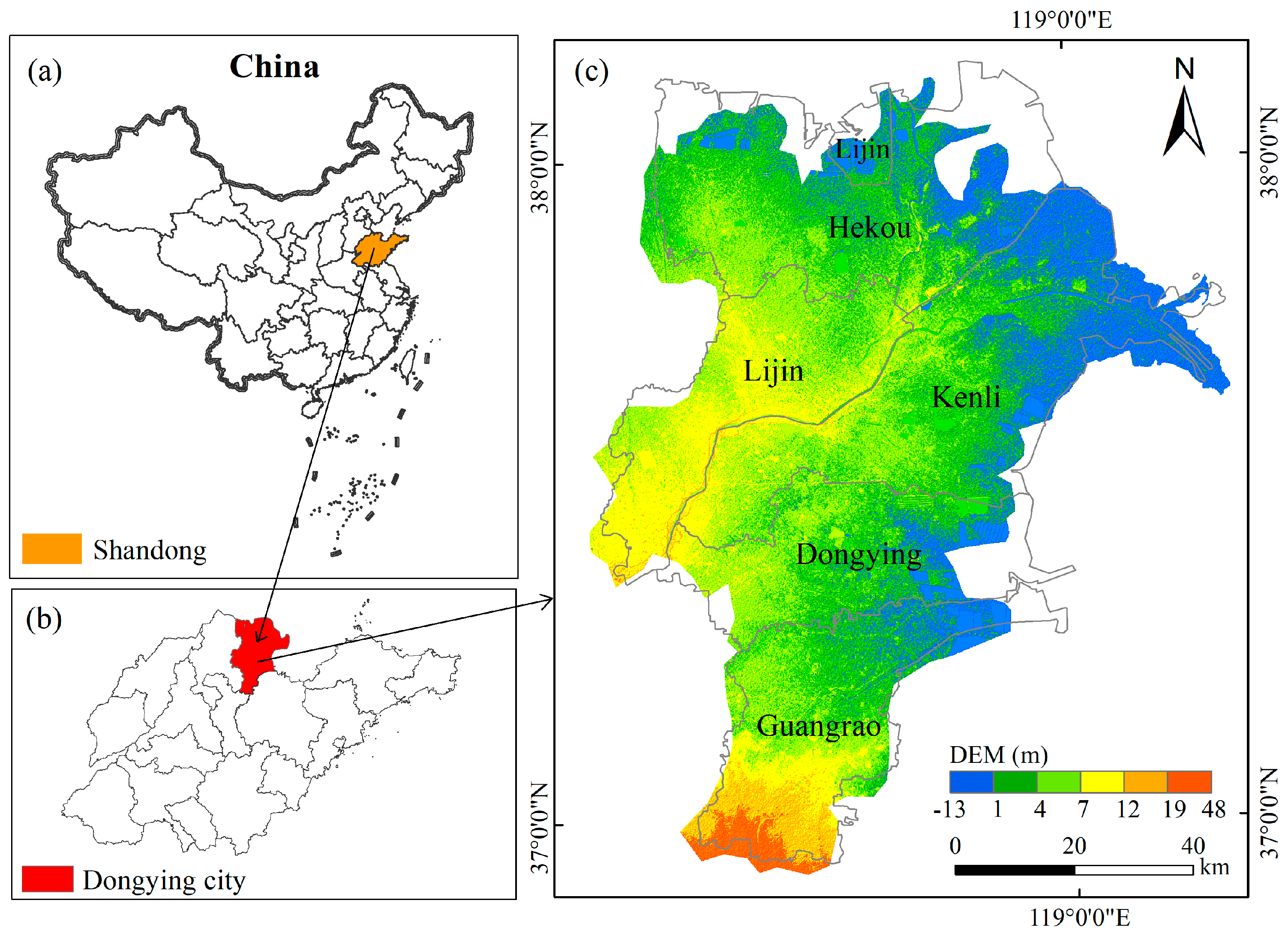
2.1. Study Area

Situated in Shandong Province’s northern section, the Yellow River Delta region is bounded by Laizhou Bay to the east and Bohai Bay to the north. Its geographic coordinates fall between 117°31′–119°18′E and 36°55′–38°16′N. A warm temperate semi-humid continental monsoon climate, with hot and rainy summers and cold dry winters, predominates, influenced by the Pacific Ocean and the Eurasian continent. There is an average of 12.6 °C in temperature and 551.6 mm of precipitation every year [22]. Shaped by the river–sea interaction, the region forms a huge fan-shaped accumulation with Lijin as the apex. The Yellow River Delta can be categorized as ancient, modern, or contemporary, depending on age differences and unique geographic features [23]. Since approximately 93% of the current YRD is situated in Dongying City, this study centers on the seaward expansion of Dongying City as the study area (Figure 1). Dongying District, Kenli District, Hekou District, Guangrao County, and Lijin County are the three urban districts and two counties that make up the city of Dongying. At present, the Yellow River Delta region suffers from numerous ecological problems, including land subsidence, water scarcity, ecological degradation, land resources competition, and natural disaster risks [20,24,25]. Urgent and effective measures are imperative to protect and restore the local ecological environment.

2.2. Remote Sensing Data

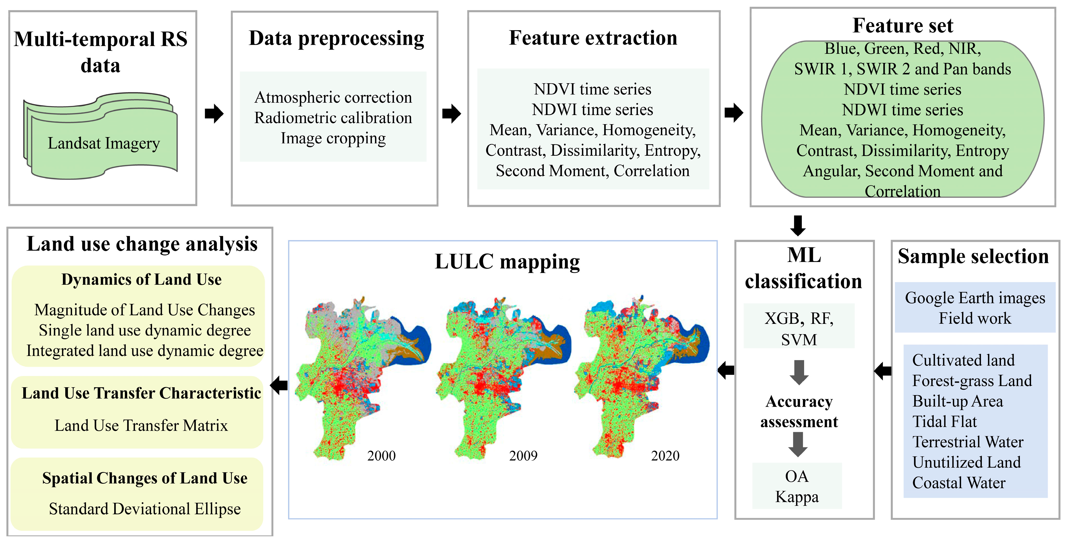
This study utilizes a total of 23 sets of Landsat TM/OLI data for the years 2000, 2009, and 2020. The datasets were obtained from the United States Geological Survey (USGS) Earth explorer (https://earthexplorer.usgs.gov/ (accessed on 10 October 2022)). The specific description of the Landsat data used are provided in

Table A1. Remote sensing image information.

Time Period	Sensor	Acquisition Time	Path/Row	Cloud Coverage (%)
2000	Landsat5 TM	20 December 2000	121/34	2.00
2000	Landsat5 TM	2 November 2000	121/34	1.00
2000	Landsat5 TM	17 October 2000	121/34	1.00
2000	Landsat5 TM	15 September 2000	121/34	4.00
2000	Landsat5 TM	8 April 2000	121/34	0.00
2000	Landsat5 TM	7 March 2000	121/34	1.00
2000	Landsat7 ETM+	9 October 2000	121/34	0.00
2000	Landsat7 ETM+	2 May 2000	121/34	1.00
2000	Landsat7 ETM+	28 February 2000	121/34	0.00
2000	Landsat7 ETM+	17 January 2000	121/34	7.00
2009	Landsat5 TM	13 December 2009	121/34	9.00
2009	Landsat5 TM	26 October 2009	121/34	2.00
2009	Landsat5 TM	3 May 2009	121/34	0.00
2009	Landsat5 TM	1 April 2009	121/34	0.00
2009	Landsat5 TM	16 March 2009	121/34	4.00
2009	Landsat5 TM	27 January 2009	121/34	2.00
2020	Landsat8 OLI	27 December 2020	121/34	5.74
2020	Landsat8 OLI	9 November 2020	121/34	0.00
2020	Landsat8 OLI	24 October 2020	121/34	0.28
2020	Landsat8 OLI	20 July 2020	121/34	0.28
2020	Landsat8 OLI	1 May 2020	121/34	0.50
2020	Landsat8 OLI	15 April 2020	121/34	5.67
2020	Landsat8 OLI	14 March 2020	121/34	0.22

in Appendix A. Images with less than 10% cloudiness in the study area were acquired to minimize atmospheric interference. All the satellite images were pre-processed using procedures such as cropping, radiometric calibration, image enhancement, etc.

3. Methodology

This study utilizes image bands, spectral index time series, and texture features in conjunction with the XGBoost (XGB) method to classify land use in the Yellow River Delta region (Figure 2). Additionally, it employs the land use transfer matrix, land use dynamic degree, and standard differential ellipse to analyze the temporal and spatial variations in land use.

3.1. Land Use Classification

Considering the land use classification standard and the degree of image decipherability, the land use/cover categories are categorized into seven types: cultivated land, forest–grassland, built-up area, tidal flats, terrestrial water (including reservoirs, ponds, saline, and rivers), unutilized land (including saline and barren land), and coastal water. The wetlands mainly consist of tidal flats, terrestrial water, and forest–grassland. Forest–grassland typically refers to sparsely vegetated grasslands and shrublands growing on moist soil such as marshes. Coastal water is near the coastline, including bays, straits, and marine areas, influenced by the ocean. Terrestrial water is water bodies away from the ocean, primarily influenced by land factors.

3.1.1. Image Features

Details of the image features for land use classification in this study are provided in

Table 1. Image features used in this study.

Type	Description
Image band	Blue, green, red, NIR, SWIR 1, SWIR 2, and pan bands
Spectral index	Normalized Difference Vegetation Index ($\mathrm{N}\mathrm{D}\mathrm{V}\mathrm{I}$) Normalized Difference Water Index ($\mathrm{N}\mathrm{D}\mathrm{W}\mathrm{I}$)
Textural feature	Homogeneity, variance, mean dissimilarity, entropy, contrast, second moments, and correlation

.

(1)

Image band

The seven bands from the Landsat images taken during the vegetation growth seasons on 2 May 2000, 3 May 2009, and 1 May 2020 include blue, green, red, near-infrared (NIR), short-wave infrared 1 (SWIR 1), short-wave infrared 2 (SWIR 2), and panchromatic (pan).

(2)

Spectral index

One vegetation index that is frequently used to identify changes in land use and cover is the Normalized Difference Vegetation Index (NDVI) [26]. Due to variations in vegetation NDVI across different months of the year, this study utilized Landsat images from the months of 2000, 2009, and 2020 to construct NDVI time series. The NDVI can be calculated using Equation (1):

$$NDVI=\frac{{\mathrm{R}}_{nir}-{\mathrm{R}}_r}{{\mathrm{R}}_{nir}+{\mathrm{R}}_r}$$

(1)

where ${\mathrm{R}}_{nir}$ and ${\mathrm{R}}_r$ stand for the reflectance values in the red and near-infrared bands, respectively.

The Normalized Difference Water Index (NDWI) is an index used for monitoring and analyzing remotely sensed water bodies [27], which can help to detect water bodies. This study uses Landsat images of the months of 2000, 2009, and 2020 to construct NDWI time series. The NDWI can be calculated using Equation (2):

$$NDWI=\frac{{\mathrm{R}}_g-{\mathrm{R}}_{nir}}{{\mathrm{R}}_g+{\mathrm{R}}_{nir}}$$

(2)

where ${\mathrm{R}}_g$ represents the reflectance value in green band.

(3)

Textural feature

Satellite image textures can provide extensive information on vegetation structure [28] and land use [29]. The gray-level co-occurrence matrix (GLCM) is a method for calculating the texture features of an image by considering the relationship between different pairs of pixel values [30]. The dataset used for textural feature calculation consists of remote sensing images captured on 2 May 2000, 3 May 2009, and 1 May 2020. The window size for texture extraction was set to 3. Eight texture features, including homogeneity, variance, mean, dissimilarity, entropy, contrast, second moments, and correlation, were calculated using the GLCM.

3.1.2. Machine Learning Methods

As a machine learning approach, the XGB (extreme gradient boosting) classifier is based on gradient boosting decision trees. It obtains strong classifiers by serially training weak classifiers, and usually performs well in classification and regression tasks. In this study, the XGBoost 1.6.2 in Python was used. To enhance the accuracy of the classification results, mathematical morphology operations were further performed on the results obtained from the XGB classification. These included expansion and erosion operations, followed by the merging of adjacent similar regions.

3.1.3. Training, Testing, and Validation

A total of 1000 samples for each land cover type were collected in the study area for each time period. For year 2020, the authors conducted field work in the study area to collect samples and determine their land use types. For 2000 and 2009, the reference samples were collected by visually interpreting historical high-resolution satellite images from Google Earth. An 8:2 ratio was used to randomly separate the samples into training and test sets (

Table 2. The reference samples for model training and validation.

Class	Training	Test
Cultivated Land	800	200
Forest–Grassland	800	200
Built-up Area	800	200
Tidal Flat	800	200
Terrestrial Water	800	200
Unutilized Land	800	200
Coastal Water	800	200
Total	5600	1400

). In this work, we used 4-fold cross-validation to determine the model’s ideal hyperparameters. Twenty percent of the samples were used for accuracy verification, while the remaining eighty percent were used to train the XGB classifier. Overall accuracy and kappa coefficients were used for land use classification accuracy evaluation.

3.2. Land Use Transfer Matrix

The direction and extent of land conversion are described by the transfer matrix [31]. It can be defined using Equation (3):

$$S_{ij}=\left[\begin{array}{cccc}{S}_{11}& S_{12}& \cdots & S_{1n}\\ S_{21}& S_{22}& \cdots & S_{2n}\\ ⋮& ⋮& ⋮& ⋮\\ S_{n1}& S_{n2}& \cdots & S_{nn}\end{array}\right]$$

(3)

where $S_{ij}$ represents an n × n matrix, $S$ represents the area of land, and $i$ and $j$ represent the land use type at the start and finish time periods, respectively.

3.3. Land Use Dynamics

3.3.1. Magnitude of Land Use Changes

The degree of change in land area is characterized by the extent of change in land use. It can be calculated using Equation (4):

$$L_t=\frac{U_b-U_a}{U_a}\times 100\%$$

(4)

where $L_t$ denotes the extent of change for the land type over the research period. The areas of a land use type at the start and finish time periods are denoted by $U_a$ and $U_b$, respectively.

3.3.2. Single Land Use Dynamic Degree

The changing rate of a certain land use type over a specified time range is indicated by the single land use dynamic degree [32] (Equation (5)):

$$K=\frac{U_b-U_a}{U_a}\times \frac{1}{T}\times 100$$

(5)

where $K$ indicates the land use dynamic degree of a land use type, and $T$ represents the study time. For a specific land use type, $K$ denotes the annual changing rate when $T$ is expressed in years.

3.3.3. Integrated Land Use Dynamic Degree

The changing rate of regional land use types can be characterized by integrated land use dynamic degrees [33]. It can be calculated using Equation (6):

$$LC=\frac{{\sum }_{i=1}^n\Delta {LU}_{i-j}}{2{\sum }_{i=1}^n{LU}_i}\times \frac{1}{T}\times 100\%$$

(6)

where $LC$ represents the pace at which the region’s land use is changing. The area transferred from land use type $i$ to $j$ is represented by the absolute value ${LU}_{i-j}$. The area of land use type $i$ at the start time point is denoted by ${LU}_i$. T refers to the length of the study period.

3.4. Standard Deviational Ellipse

The standard deviational ellipse is able to represent the spatial concentration trend, discrete trend, and directional distribution of geographic elements [33]. The three main features of the standard deviational ellipse include the long axis $x$ (standard deviation along the major axis), the short axis $y$ (standard deviation along the minor axis), and the angle of rotation $\theta$. The variance of the long and short semi-axes can be calculated using Equation (7):

$$\left.\begin{array}{l}SDEx=\sqrt{\frac{{\sum }_{i=1}^n{\left(x_i - \bar{x}\right)}^2}{n}}\\ {SDE}_y=\sqrt{\frac{{\sum }_{i=1}^n{\left(y_i - \bar{y}\right)}^2}{n}}\end{array}\right\}$$

(7)

where $SDEx$ and $SDEy$ represent the variance of the long and short semi-axes, respectively. $x_i$ and $y_i$ are the spatial location coordinates of each element. $\bar{x}$ and $\bar{y}$ are arithmetic mean centers.

The tangent of rotation angle can be calculated using Equation (8):

$$tan \theta =\frac{\sum _{i=1}^n{\tilde{x}}_i^2-\sum _{i=1}^n{\tilde{y}}_i^2+\sqrt{{\left(\sum _{i=1}^n{\tilde{x}}_i^2-\sum _{i=1}^n{\tilde{y}}_i^2\right)}^2+4{\left(\sum _{i=1}^n{\tilde{x}}_i{\tilde{y}}_i\right)}^2}}{2\sum _{i=1}^n{\tilde{x}}_i{\tilde{y}}_i}$$

(8)

where $\theta$ represents the angle of rotation, clockwise to the $x$-axis in the north direction. $\tilde{x}$ and ${\tilde{y}}_i$ are the mean central deviations.

The standard deviation can be calculated using Equation (9):

$$\left.\begin{array}{rr}{\sigma }_x& =\sqrt{2}\sqrt{\frac{{\sum }_{i=1}^n{\left({\tilde{x}}_i\mathrm{c}\mathrm{o}\mathrm{s} \theta - {\tilde{y}}_i\mathrm{c}\mathrm{o}\mathrm{s} \theta \right)}^2}{n}}\\ {\sigma }_y& =\sqrt{2}\sqrt{\frac{{\sum }_{i=1}^n{\left({\tilde{x}}_i\mathrm{s}\mathrm{i}\mathrm{n} \theta + {\tilde{y}}_i\mathrm{c}\mathrm{o}\mathrm{s} \theta \right)}^2}{n}}\end{array}\right\}$$

(9)

where ${\sigma }_x, {\sigma }_y$ represent the standard deviation of the $x$- and $y$-axes, respectively.

4. Results

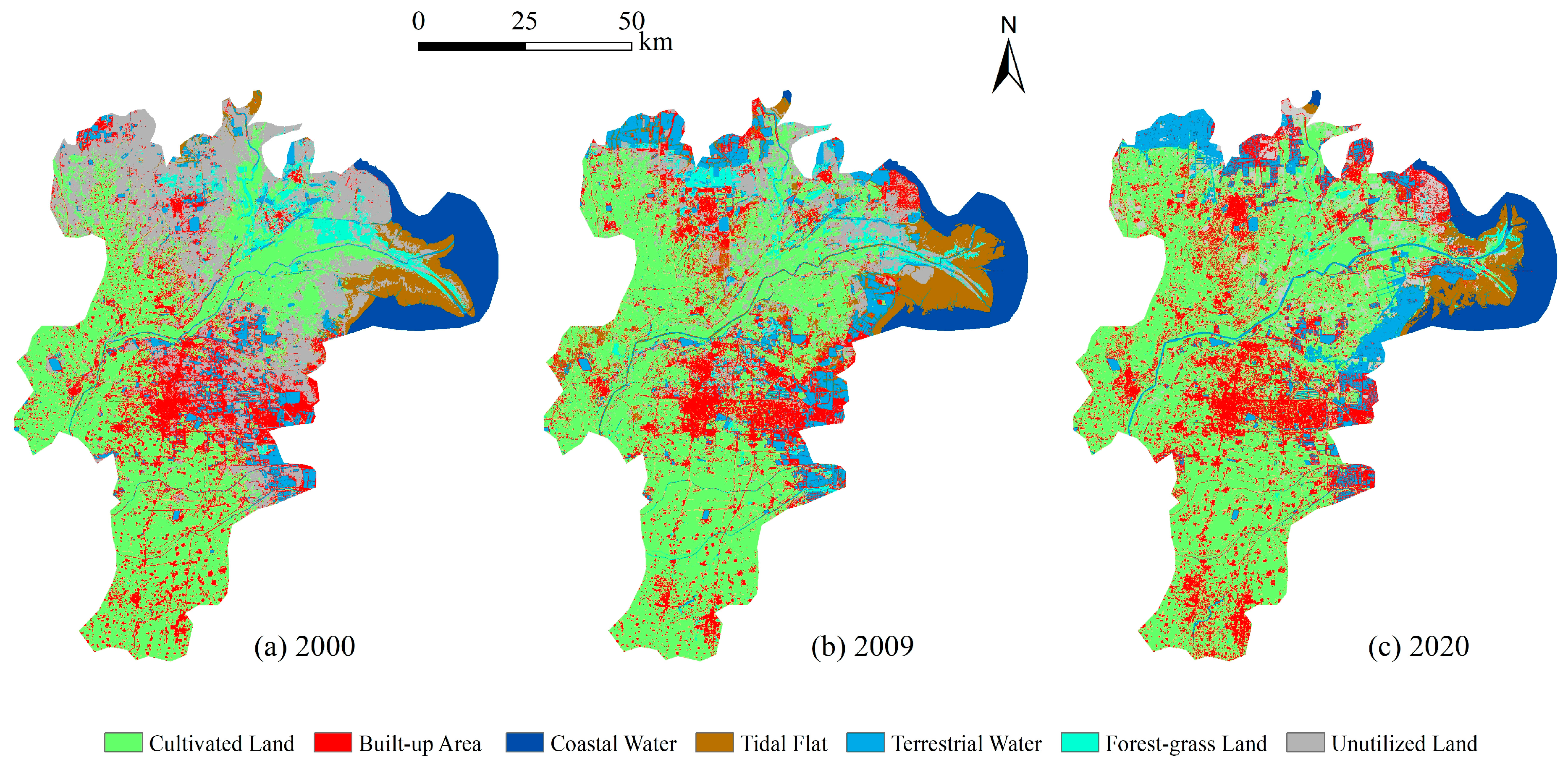
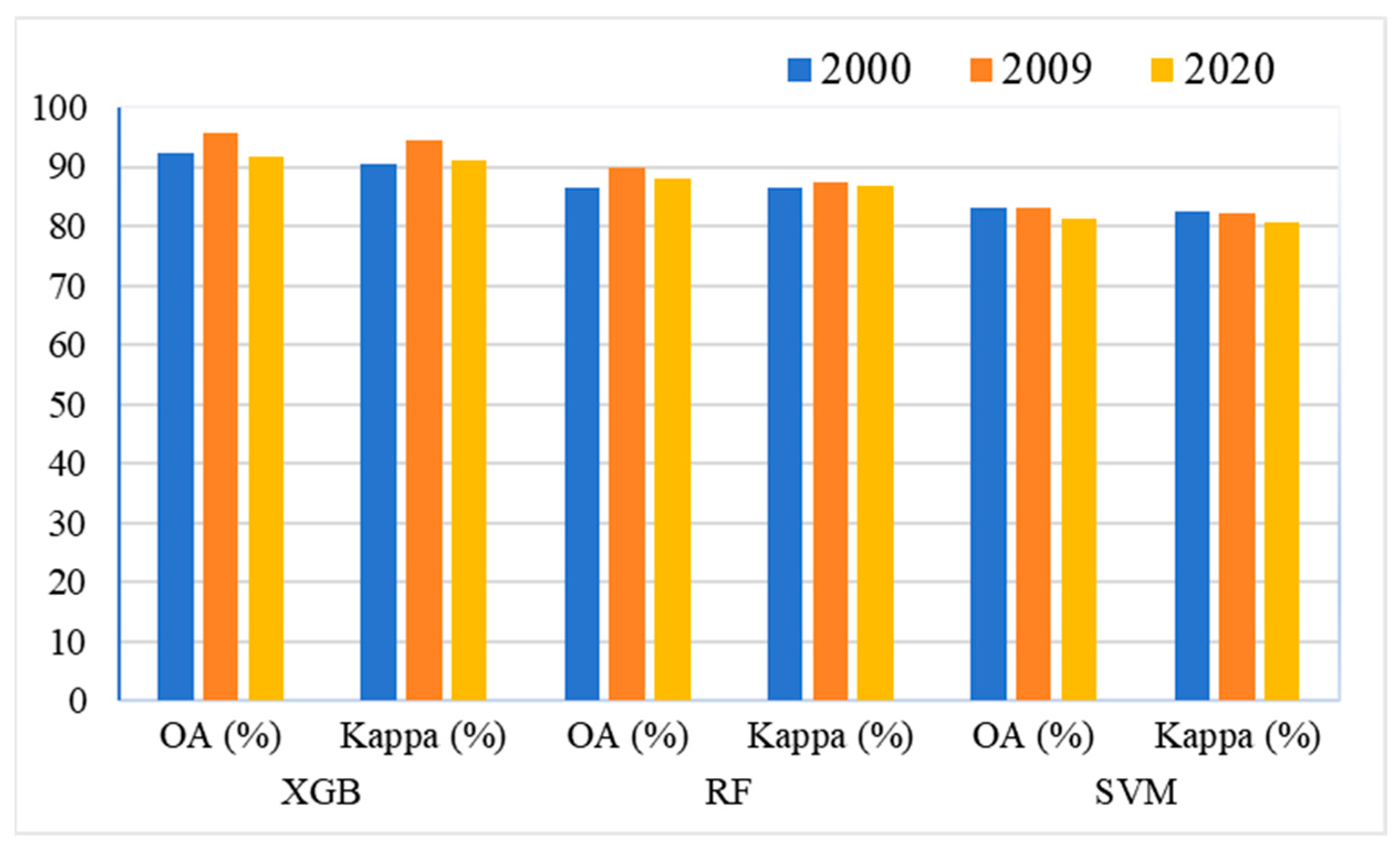
4.1. Land Use Classification and Distribution

The land use classification results for 2000, 2009, and 2020 were obtained using Landsat remote sensing images (Figure 3). The area and proportion of each land use type were obtained in different periods (

Table 3. Land use structures in the Yellow River Delta from 2000 to 2020.

Land Use Type	2000		2009		2020
	Area (km2)	Proportion (%)	Area (km2)	Proportion (%)	Area (km2)	Proportion (%)
Tidal Flat	227.47	3.09	543.03	7.37	269.11	3.65
Cultivated Land	3451.75	46.84	3388.80	45.98	3829.46	51.95
Coastal Water	500.05	6.79	424.98	5.77	463.95	6.29
Built-up Area	931.02	12.63	1193.98	16.20	1564.04	21.22
Forest–Grassland	248.60	3.37	336.65	4.57	76.97	1.04
Terrestrial Water	467.25	6.34	672.56	9.13	753.81	10.23
Unutilized Land	1543.66	20.95	810.21	10.99	413.70	5.61
Other Land Types	1.24	0.02	0.85	0.01	0.0031	0.00
Total Area	7371.04	100.00	7371.04	100.00	7371.04	100.00

) by analyzing the multi-temporal land use maps. Cultivated land is the main land use type in the study area, with an area and share of more than 45%. It shows a decreasing and then increasing trend. The areas of built-up area and terrestrial water are increasing. The area of unutilized land is decreasing. The YRD’s acreage has grown and expanded eastward during the last 20 years, while the sea area has shrunk. Tidal flats are mainly found around sea areas, salt flats, and ponds. A small portion is found along inland rivers and lakes. The majority of the croplands are located along the Yellow River and in the study area’s southwest and south. The majority of built-up area is located in the study area’s center, where it is progressively growing to the periphery while agriculture is scattered throughout. The Yellow River Delta Nature Reserve and the area close to the river’s mouth are home to the majority of the forest–grassland. Most of the vacant land is located in the estuary and along the coast.

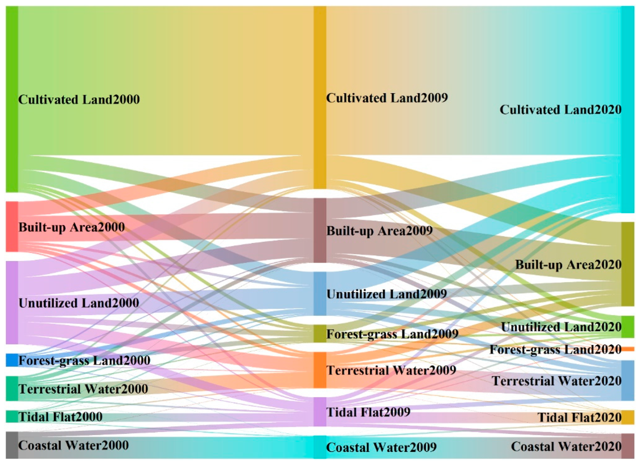
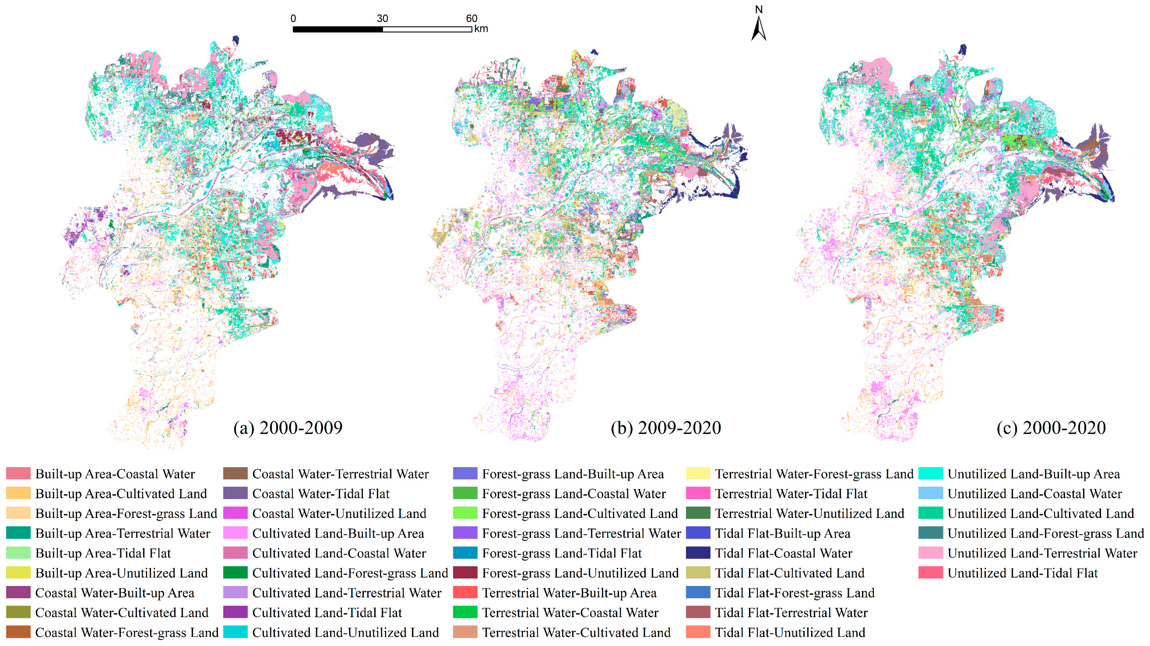
4.2. Land Use Transfer Characteristic

The transfer matrix is used to examine the land use changes in the Yellow River Delta region. Detailed statistical analysis results are provided in

Table A2. Transfer matrix among land use categories from 2000 to 2009.

From 2000 to 2009	Tidal Flat	Cultivated Land	Coastal Water	Built-Up Area	Forest–Grassland	Terrestrial Water	Unutilized Land	Total in 2009	Transfer to
Tidal Flats	159.45	65.41	90.03	23.19	12.99	29.55	162.35	542.97	383.52
Cultivated Land	1.79	2762.26	0.02	262.68	28.45	36.26	297.14	3388.59	626.33
Coastal Water	14.13	0.13	403.26	0.02	0.73	1.87	4.77	424.93	21.66
Built-up Area	6.64	266.64	0.59	478.08	16.39	80.22	345.03	1193.58	715.51
Forest–Grassland	5.60	71.00	0.68	45.02	87.48	20.48	106.36	336.61	249.13
Terrestrial Water	8.31	41.26	4.83	72.56	15.34	274.51	245.57	672.39	397.88
Unutilized Land	21.54	244.84	0.61	49.37	87.20	24.30	382.28	810.13	427.86
Total in 2000	227.46	3451.54	500.03	930.91	248.58	467.19	1543.50	7369.21
Transfer Out	68.01	689.28	96.76	452.83	161.10	192.67	1161.22

,

Table A3. Transfer matrix among land use categories from 2009 to 2020.

From 2009 to 2020	Tidal Flat	Cultivated Land	Coastal Water	Built-Up Area	Forest–Grassland	Terrestrial Water	Unutilized Land	Total in 2020	Transfer to
Tidal Flats	200.73	8.18	26.04	2.88	9.04	11.86	10.36	269.10	68.37
Cultivated Land	85.33	2759.65	0.09	375.99	149.82	60.78	397.61	3829.27	1069.63
Coastal Water	63.50	0.06	396.60	0.29	0.44	2.90	0.13	463.93	67.32
Built-up Area	64.61	446.41	0.60	643.84	79.26	162.38	166.44	1563.54	919.70
Forest–Grassland	15.19	13.17	0.89	5.83	24.07	3.02	14.81	76.97	52.90
Terrestrial Water	84.34	52.30	0.74	92.42	34.97	389.92	99.00	753.70	363.77
Unutilized Land	29.33	109.03	0.01	72.72	39.04	41.69	121.84	413.66	291.81
Total in 2009	543.03	3388.79	424.98	1193.97	336.64	672.55	810.20	7370.17
Transfer Out	342.30	629.15	28.37	550.13	312.57	282.63	688.36

and

Table A4. Transfer matrix among land use categories from 2000 to 2020.

From 2000 to 2020	Tidal Flat	Cultivated Land	Coastal Water	Built-Up Area	Forest–Grassland	Terrestrial Water	Unutilized Land	Total in 2020	Transfer to
Tidal Flats	108.10	7.67	74.57	1.89	10.81	8.14	57.90	269.09	160.98
Cultivated Land	8.90	2742.02	1.89	320.92	116.44	84.33	554.73	3829.23	1087.20
Coastal Water	40.23	0.29	405.22	0.17	2.67	4.19	11.13	463.90	58.68
Built-up Area	13.21	478.59	1.45	500.37	40.30	149.73	379.69	1563.34	1062.98
Forest–Grassland	5.91	14.08	11.94	2.94	23.33	2.86	15.92	76.97	53.64
Terrestrial Water	39.26	89.41	3.79	78.47	18.31	195.69	328.68	753.62	557.93
Unutilized Land	11.86	119.68	1.19	26.25	36.74	22.31	195.60	413.63	218.03
Total in 2000	227.47	3451.75	500.04	931.01	248.60	467.25	1543.65	7369.77
Transfer out	119.37	709.72	498.60	904.76	225.27	271.56	1348.06

in Appendix A. There has been a significant shift in land use types over the past 20 years, mainly between unutilized land, built-up area, cultivated land, and terrestrial water (Figure 4). More land area was transferred to cultivated land in 2009–2020 than in 2000–2009. Tidal flats increased and then decreased from 2000 to 2020, increasing by 41.63 km². The land transferred to the tidal flats is mainly coastal and unutilized land. Cultivated land decreased and then increased, increasing by a total of 377.71 km². Unutilized land, built-up area, and forest–grassland are the main sources of cultivated land. Built-up area increased by 633.03 km², and the land transferred to built-up area mainly came from cultivated land, unutilized land, and terrestrial water. Forest–grassland increased and then decreased, with a net decrease of 171.63 km². It was mainly converted to cultivated land, built-up area, and unutilized land. Terrestrial water increased by 286.57 km², mainly from unutilized land, cultivated land, and built-up area. Unutilized land decreased by 1129.96 km², mainly converted to cultivated land, built-up area, and terrestrial water.

The spatial pattern of land use conversion in the study area between 2000 and 2020 is displayed in Figure 5. Wetlands include artificial wetlands dominated by terrestrial waters and natural wetlands dominated by rivers, lakes, tidal flats, and forest–grassland. Between 2000 and 2020, most of the land converted to wetlands was distributed along the Yellow River and the region where the Yellow River flows into the sea. Cultivated land converted to tidal flats is mostly distributed along the Yellow River. Interchange occurs between tidal flats, forest–grassland, and terrestrial water in the Yellow River estuary. Tidal flats in the Yellow River estuary area have increased, with more coastal water being converted to tidal flats than tidal flats to coastal water. Wetlands are mainly distributed in the Hekou and Kenli districts. The Hekou district mainly consists of artificial wetlands, such as ponds and reservoirs. Both artificial wetlands and natural wetlands are distributed in the Kenli District. From 2000–2009, large areas of unutilized land were converted to terrestrial water in the Hekou District, the northern part of Lijin County, and the eastern part of Kenli District, leading to an increase in artificial wetlands. From 2009–2020, part of the unutilized land became terrestrial water in the eastern Kenli District. Constrained by the influx of water and sand from the Yellow River, the area of the tidal flats has diminished. Since measures such as protecting wetlands and developing unutilized land as wetlands have been implemented, the area of wetlands has not been significantly reduced. The Hekou District, Lijin County, and the Kenli District have achieved remarkable results in wetland protection. Before 2009, the wetlands in the area were not properly planned and allowed to develop freely. There is a large amount of unutilized land. After 2009, part of the unutilized land in the Yellow River Estuary Ecotourism Zone was converted into built-up area. This shows that wetland protection has attracted people’s attention, so a large amount of unutilized land has been transformed into wetlands. Artificial wetlands, mainly terrestrial water, and natural wetlands, represented by forest–grassland and tidal flats, have been rationally planned and laid out. This contributes to ecosystem stability and has a positive impact on wetland conservation.

Table 4. Area, magnitude, and dynamic degree of land use changes between 2000 and 2020 in the Yellow River Delta.

Land Use Type	2000–2009			2009–2020			2000–2020
	Areal Change/km2	${\mathit{L}}_{\mathit{t}}$	$\mathit{K}$	Areal Change/km2	${\mathit{L}}_{\mathit{t}}$	$\mathit{K}$	Areal Change/km2	${\mathit{L}}_{\mathit{t}}$	$\mathit{K}$
Tidal Flat	315.55	138.72%	13.87%	−273.92	−50.44%	−4.59%	41.63	15.47%	0.87%
Cultivated Land	−62.95	−1.82%	−0.18%	440.66	13.00%	1.18%	377.71	9.86%	0.52%
Coastal Water	−75.07	−15.01%	−1.50%	38.96	9.17%	0.83%	−36.1	−7.78%	−0.34%
Built-up Area	262.96	28.24%	2.82%	370.07	30.99%	2.82%	633.03	40.47%	3.24%
Forest–Grassland	88.05	35.42%	3.54%	−259.67	−77.14%	−7.01%	−171.63	−222.98%	−3.29%
Terrestrial Water	205.31	43.94%	4.39%	81.26	12.08%	1.10%	286.57	38.02%	2.92%
Unutilized Land	−733.46	47.51%	−4.75%	−396.51	−48.94%	−4.45%	−1129.96	−273.14%	−3.49%
$LC$	1.91%			1.92%			1.09%

illustrates the changes in land use types in the Yellow River Delta region. Other landforms are not discussed in this paper due to their small proportions. The land use types that increased (positive K-value) are mainly built-up area, terrestrial water, tidal flats, and cultivated land. The increasing area in descending order is built-up area, terrestrial water, and cultivated land, with values of 3.24%, 2.92%, and 0.52%, respectively. The land use types that decreased (negative K-value) are coastal water, forest–grassland, and unutilized land. The decreasing area, in descending order, is unutilized land, forest–grassland, and coastal water, with values of −3.49%, −3.29%, and −0.34%, respectively. The K-value was positive only for built-up area and terrestrial water in all intervals of time. Cultivated land had a negative K-value and then a positive K-value, with an increase in total area. The K-value of tidal flats was positive and then negative, and the total area increased. The K-value of unutilized land was always negative. The K-value of coastal water was negative and then positive, and the total area decreased. Forest–grassland had a positive K-value at first, but eventually it turned negative, and its overall area drastically shrunk. The combined land use dynamics were 1.91% for 2000–2009, 1.92% for 2009–2020, and 1.09% for 2000–2020 in terms of integrated land use dynamics.

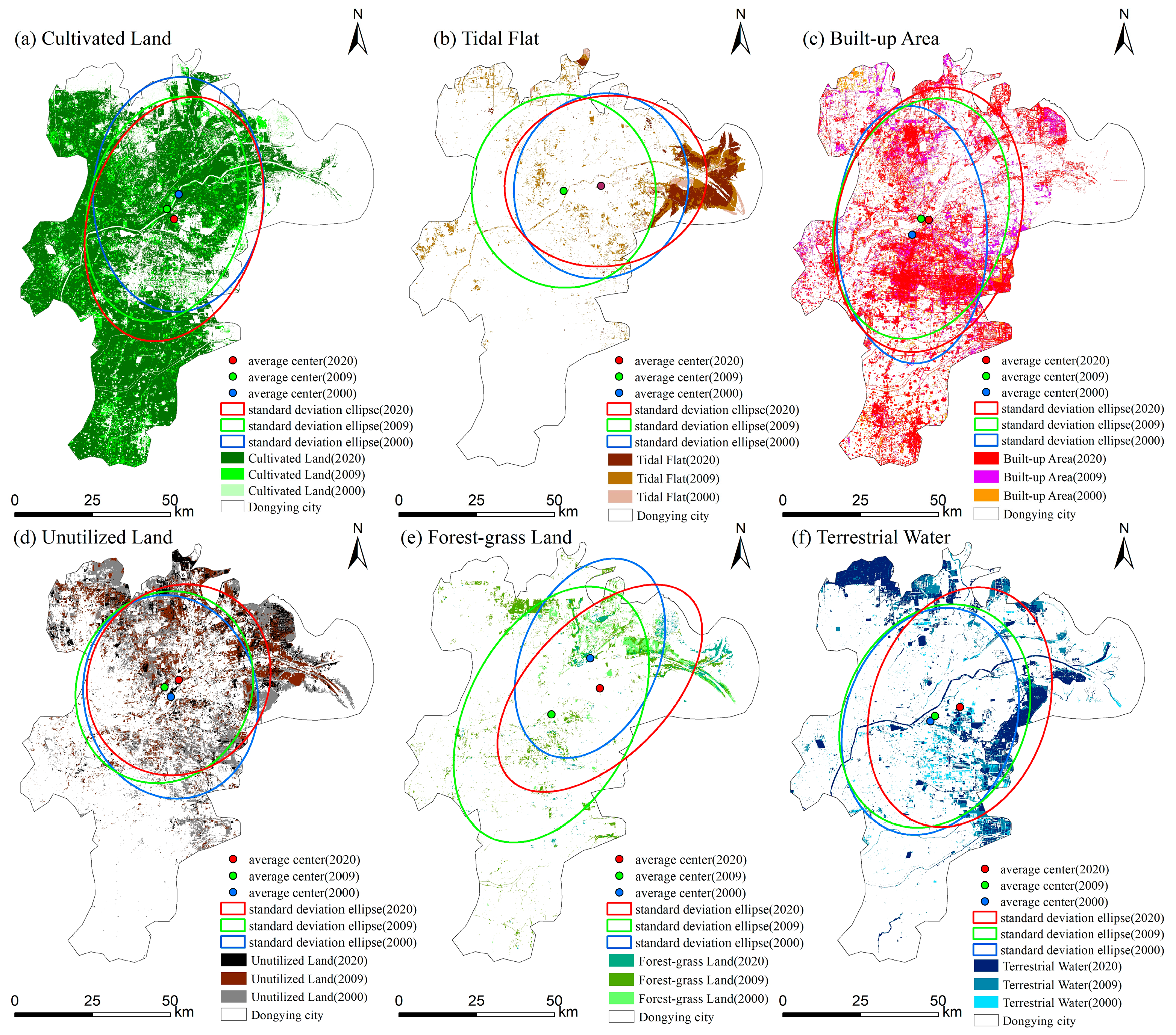
4.3. Spatial Changes of Land Use

In order to investigate the changing pattern and direction of each land use type, the standard deviation ellipse was created (Figure 6). Detailed parameters are given in

Table A5. Standard deviation ellipse parameters for various land use types over time.

Land Use Categories	Year	Circumference (km)	Area (km2)	X-Coordinate of Centroid (km)	Y-Coordinate of Centroid (km)	Short Axis (km)	Long Axis (km)	Orientation Angle (°)	Ellipticity
Cultivated Land	2000	205.77	3247.25	646,798.96	4,174,407.97	27,464.64	37,637.21	2.15	0.07
	2009	196.21	2905.03	643,006.59	4,169,677.33	25,163.44	36,749.99	15.35	0.08
	2020	213.99	3452.67	645,325.56	4,166,492.82	27,394.74	40,120.42	17.35	0.08
Tidal Flats	2000	181.00	2610.80	657,651.53	4,177,004.91	27,739.98	29,959.82	21.17	0.02
	2009	190.26	2877.88	645,618.06	4,175,339.75	29,542.20	31,009.98	170.30	0.01
	2020	188.32	2787.19	659,094.67	4,178,532.00	27,192.11	32,628.44	79.64	0.04
Built-up Area	2000	209.05	3130.45	634,686.96	4,161,262.76	24,143.63	41,274.99	178.39	0.10
	2009	210.99	3376.20	637,611.91	4,166,429.24	27,384.55	39,246.40	15.24	0.08
	2020	229.60	3969.69	640,040.13	4,166,034.79	29,307.79	43,117.26	14.11	0.08
Terrestrial Water	2000	203.15	3171.88	640,818.70	4,163,902.54	27,271.67	37,023.78	18.24	0.07
	2009	207.87	3364.95	642,301.48	4,165,580.94	29,019.99	36,910.93	25.05	0.05
	2020	213.17	3470.62	650,257.66	4,168,391.28	28,150.52	39,246.16	18.73	0.07
Forest–Grassland	2000	175.37	2284.24	655,311.21	4,183,997.58	21,722.14	33,474.80	24.01	0.09
	2009	225.26	3695.29	642,909.31	4,166,079.58	26,826.85	43,848.96	27.54	0.10
	2020	202.78	2858.72	658,418.13	4,174,417.75	22,238.98	40,920.71	44.46	0.11
Unutilized Land	2000	191.08	2876.53	644,248.64	4,172,020.20	27,888.25	32,833.78	167.41	0.04
	2009	186.26	2747.38	642,200.81	4,175,107.73	27,934.18	31,307.99	24.59	0.03
	2020	188.85	2829.25	646,799.08	4,177,460.38	28,685.99	31,395.97	33.36	0.02

of Appendix A. From 2000 to 2020, cultivated land was tilted in a north–south direction, and gradually shifted to a northeast–southwest direction, with a more pronounced directionality. The mean center shifted to the south. The directionality of the spatial distribution of the tidal flats was not significant, and the mean center did not change obviously. The built-up area’s major axes skewed from northwest to northeast. The mean center shifted to the northeast. The spatial distribution ranges gradually expanded, and the pattern tended to be discrete. The orientation weakened. The major axis of the terrestrial water extended in a northeasterly direction. The mean center shifted to the northeast. The spatial distribution extent gradually expanded and the pattern tended to be decentralized. The orientation of the spatial distribution was first weakened and then obvious. Forest–grassland gradually shifted to the northeast–southwest direction and the orientation became more pronounced. The mean center shifted to the southeast. The spatial distribution tended to be discrete and then centralized. The unutilized land’s major axis shifted from northwest to northeast. The mean center moved to the northeast. The directionality of the spatial distribution was gradually significant, and the area first decreased sharply and then increased. From 2000 to 2009, the development of unutilized land led to a decrease, and from 2009 to 2020, because of the worsening of soil salinity, part of the cultivated land was changed into unutilized land, which led to an area increase.

The standard deviation ellipse parameters for various terrain types are shown in Figure 7 as a variation of the long axis, short axis, short axis/long axis, and angle. The lengths of the short and long axes indicate the degree of dispersion of the data in the secondary and primary directions, respectively. As seen in Figure 7a,b, from 2000 to 2020, the short and long axes of forest–grassland both rise first and then fall, which indicates that the distribution of forest–grassland is first discrete and then aggregated. From 2000 to 2009, a portion of the widely distributed unutilized land and cultivated land in the region was transformed into forest–grassland. From 2009 to 2020, there was a conversion of unutilized land and tidal flats near the Yellow River estuary into forest–grassland, and during the same period, forest–grassland in the inland area decreased while the distribution of forest–grassland became more aggregated. The short/long axis characterizes the flatness of the data distribution. According to Figure 7c, the short/long axis of both unutilized land and tidal flats is greater than 0.8, indicating that the distribution of unutilized land and tidal flats is strongly concentrated in a certain direction. Combined with Figure 6, it is clear that the unutilized land is more concentrated in the north–south direction. Mudflats are found primarily in an easterly orientation. The direction angle shows the angle formed by the ellipse’s main axis and the direction of due north. As illustrated in Figure 7d, between 2000 and 2009, the angle of the direction of built-up and unutilized area decreased, getting closer to 0° and 180°, indicating that the data are still spread along a north–south axis. Combined with Figure 6, it can be seen that the distribution of unutilized land gradually shifted due north, while the distribution of built-up area moved to the north and south. The angle of the tidal flats shifted from near 0° and 180° to nearly 90°, suggesting that the tidal flat distribution shifted from a north–south to an east–west direction. This is due to the increase in tidal flats at the mouth of the Yellow River Delta.

5. Discussion

5.1. Land Use Classification Method

Previous studies have often relied on pre-existing land use/cover products for land change analyses [34]. While these products are suitable for monitoring long-term change and have the advantage of easier access, they may suffer from a lack of classification accuracy as well as missing data. Furthermore, the application of large-scale land use data to mesoscale areas can limit the analysis [35]. Therefore, this study combines image features with machine learning classification using Landsat remote sensing imagery. With the advantages of low computational resource requirements and high efficiency [36], machine learning methods have wide applications in land use classification. Among machine learning algorithms, as an effective, adaptable, and scalable gradient boosting algorithm, XGBoost is becoming increasingly popular in the remote sensing field. Most studies have been conducted using support vector machines [37] and random forest [38] for land use/cover classification. Although SVM and RF are superior in many ways, XGBoost performs better on many datasets, handles category imbalances better, and is able to achieve higher accuracy [39,40,41]. In this study, RF and SVM methods were used for a comparative analysis using the same input features as XGBoost. The OA and kappa coefficients of different classifiers are shown in Figure 8. The results indicate that the XGBoost method obtained an overall accuracy and kappa coefficients both exceeding 90%, while RF and SVM’s overall accuracy and kappa coefficients were both below 90%.

5.2. Spatial Differentiation of Land Use Change

Over the past two decades, the YRD region has witnessed substantial changes in land use, particularly in unutilized land, built-up area, cultivated land, and terrestrial water. The relatively stable wetland areas, along with the strategic layout of both artificial and natural wetlands, contribute to the stability of the overall ecosystem. Such results are intricately tied to the city’s efforts in wetland conservation. In 2008, the Shandong provincial government formulated the “Development Plan for the High-Efficiency Eco-Economic Zone in the Yellow River Delta of Shandong Province” and issued the “Opinions on Supporting the Good and Fast Development of the Zone”. The High-Efficiency Eco-Economic Zone covers the entire area of Dongying city. The establishment of the Yellow River Delta High-Efficiency Eco-Economic Zone in 2009, along with the implementation of its development plan, prioritized high-efficiency and eco-economic growth. The implementation of wetland restoration and protection projects, as well as water system connectivity initiatives, along with the construction of natural reserve areas, wetland parks, forest parks, etc., integrates ecological protection and restoration into the entirety of urban planning and construction management processes. To protect the new estuarine wetlands of the Yellow River Delta Nature Reserve (YRDNR), the Yellow River Conservancy Commission decided, in 2008, to directly deliver fresh water from the YR to estuarine wetlands within the reserve [42]. Both the wetland areas and their ecosystem parameters have significantly improved [43]. The stability of wetland areas and ecosystems reflects the outcomes of wetland protection efforts. Zhang et al. found that the habitat quality in 2020 increased compared to that in 2011, which is mainly due to the background of the major strategy of ecological protection and high-quality development of the Yellow River basin and the continuous ecological replenishment work since 2008. More policies and management measures have been implemented to strengthen the protection of the Yellow River Delta Wetland [44]. This aligns with the findings of a previous study, indicating an increase in water flow into wetlands since 2000 and the effectiveness of artificial wetlands in preventing wetland degradation [45]. Zhang found that, from 2006 to 2018, as environmental policies were implemented and wetland protection became more important, the rate of development of wetland areas increased in a north–south direction, the proportion of landscape types became more balanced, and the spatial distribution homogenized [46]. Yin et al. found that cultural services within the various ecosystem services of the Yellow River Delta wetlands are generally in harmony with other ecosystem services, indicating a relatively stable relationship between humans and wetlands in this region [47]. This is consistent with the improvement in the stability of wetland ecosystems revealed in this study.

The predominant land use type is cultivated land, with an increasing built-up area and decreasing unutilized land from 2000 to 2020. The increased built-up land was primarily converted from cultivated and unutilized areas. This aligns with a previous study indicating that from 2000 to 2018, cultivated land remained dominant while built-up areas expanded, mainly through the conversion of cultivated and unutilized land [48]. Our study revealed a transformation of unutilized and built-up areas into cultivated land, initially decreasing before experiencing subsequent growth, resulting in a substantial overall increase in cultivated land. The reason for this is that, in 2008, the Dongying municipal government established efficient demonstration zones for unutilized land, fostering significant development and land transfers. This strategy aimed to foster economic expansion while protecting cultivated land areas. Economically, the Yellow River Delta region boasts abundant natural resources like oil, natural gas, and salt, coupled with a strategic location advantage. The thriving marine economy and expanding port infrastructure significantly drive economic growth, attracting more laborers and boosting population numbers. This demographic surge increases the demand for food. In addition, technological developments in agriculture improve productivity by making it easier to use land that was previously idle and hastening the transformation of different kinds of land into cultivated areas. Advancements in saline land management technology have enhanced the utilization of previously unutilized land, thereby helping safeguard the quantity of cultivated land to some extent. For the changes in built-up areas, urban and rural planning authorities may rearrange some construction land that is no longer used or undeveloped as agricultural land. Some salinized cropland has been abandoned and converted into forest–grassland.

Unutilized land and built-up areas stretch north–south, with unutilized land migrating directly northward and built-up areas spreading in a north–south fashion. This hints at faster development in the southern region due to the transformation of unutilized land into alternative land uses. Tidal flats are distributed east–west due to the Yellow River’s geographic location and that of its estuary. The annual rate and scale of land use change are significant and accelerating. From 2009 to 2020, compared to the previous decade, there was a slight decrease in overall land use dynamics, accompanied by a slower pace of change across different land use types. This transition was driven by the rise of high-tech industries and the optimization of industrial structure, which have elevated the tertiary sector as the primary driver of regional economic growth.

5.3. Limitations and Future Directions

Using a variety of techniques, this study was able to determine the land use change’s temporal and spatial distribution pattern in the YRD region. However, there are still limitations that need to be improved. The data utilized in this paper have a spatial resolution of 30 m and a temporal scale of 10 years, indicating a relatively coarse spatial and temporal resolution. Future research could consider integrating multi-source remote sensing data to enhance data quality. The classification methods employed lack input feature selection and a comparison of multiple models, potentially impacting classification accuracy and the attainment of optimal results. In order to better understand the complex interaction between land use change and socioeconomic issues, future research might explore the reasons behind the land use changes.

6. Conclusions

This study examined in depth the changes in land use in the YRD region using time series of Landsat data from the past twenty years. The land use classification reached an accuracy of 90.45% based on Landsat time series data and XGB methods. Significant land use/cover type conversion was revealed in the study area between 2000 and 2020, primarily involving unutilized land, built-up area, cultivated land, and terrestrial water. The changing rates varied across different time periods. The areas of built-up area, cultivated land, terrestrial water, and tidal flats increased, while those of unutilized land, forest–grassland, and coastal water decreased. Built-up area and terrestrial water sustained accelerated growth, whereas unutilized land consistently decreased at a decelerated rate.

The spatial distribution of land use/cover categories saw a considerable change between 2000 and 2020. Built-up area, cultivated land, terrestrial water, and forest–grassland showed a clear orientation, oscillating mainly between the east and north directions. Tidal flats and unutilized land lacked a distinct spatial distribution. The mean centers of cultivated land and forest–grassland shifted southeastward, while those of unutilized land, built-up area, and terrestrial water shifted northeastward, with no significant shift observed for tidal flats.

From 2000 to 2020, wetland area in the YRD initially increased, and then slightly decreased. Overall, over the past two decades, there has been a notable increase in wetland area. This expansion is marked by the significant conversion of unutilized land into both artificial and natural wetlands, reflecting the positive effects in conservation and restoration efforts. This transformation led to a diversified wetland composition and an improved ecological environment. After 2009, the protection and restoration efforts in nature reserves, such as wetland ecological restoration and coastal zone protection projects, yielded remarkable positive outcomes.

References

1. Wang, H.; Liu, Y.; Wang, Y.; Yao, Y.; Wang, C. Land Cover Change in Global Drylands: A Review. Sci. Total Environ. 2023, 863, 160943. [Google Scholar] [CrossRef]
2. Grimm, N.B.; Faeth, S.H.; Golubiewski, N.E.; Redman, C.L.; Wu, J.; Bai, X.; Briggs, J.M. Global Change and the Ecology of Cities. Science 2008, 319, 756–760. [Google Scholar] [CrossRef]
3. Huang, C.; Zhang, C.; He, Y.; Liu, Q.; Li, H.; Su, F.; Liu, G.; Bridhikitti, A. Land Cover Mapping in Cloud-Prone Tropical Areas Using Sentinel-2 Data: Integrating Spectral Features with Ndvi Temporal Dynamics. Remote Sens. 2020, 12, 1163. [Google Scholar] [CrossRef]
4. Edgeworth, F.Y. On the Probable Errors of Frequency-Constants. J. R. Stat. Soc. 1908, 71, 381–397. [Google Scholar] [CrossRef]
5. Mahalanobis, P.C. On the Generalized Distance in Statistics. Sankhyā Indian J. Stat. Ser. A (2008-) 2018, 80, S1–S7. [Google Scholar]
6. Hearst, M.A.; Dumais, S.T.; Osuna, E.; Platt, J.; Scholkopf, B. Support Vector Machines. IEEE Intell. Syst. Their Appl. 1998, 13, 18–28. [Google Scholar] [CrossRef]
7. Quinlan, J.R. Simplifying Decision Trees. Int. J. Man-Mach. Stud. 1987, 27, 221–234. [Google Scholar] [CrossRef]
8. Bengio, Y. Learning Deep Architectures for AI. Found. Trends Mach. Learn. 2009, 2, 1–127. [Google Scholar] [CrossRef]
9. Wilkinson, G.G. Results and Implications of a Study of Fifteen Years of Satellite Image Classification Experiments. IEEE Trans. Geosci. Remote Sens. 2005, 43, 433–440. [Google Scholar] [CrossRef]
10. LeCun, Y.; Bengio, Y.; Hinton, G. Deep Learning. Nature 2015, 521, 436–444. [Google Scholar] [CrossRef] [PubMed]
11. Kussul, N.; Lavreniuk, M.; Skakun, S.; Shelestov, A. Deep Learning Classification of Land Cover and Crop Types Using Remote Sensing Data. IEEE Geosci. Remote Sens. Lett. 2017, 14, 778–782. [Google Scholar] [CrossRef]
12. Zhong, L.; Hu, L.; Zhou, H. Deep Learning Based Multi-Temporal Crop Classification. Remote Sens. Environ. 2019, 221, 430–443. [Google Scholar] [CrossRef]
13. Ball, J.E.; Anderson, D.T.; Chan, C.S. Comprehensive Survey of Deep Learning in Remote Sensing: Theories, Tools, and Challenges for the Community. J. Appl. Remote Sens. 2017, 11, 042609. [Google Scholar] [CrossRef]
14. Marcelo Acha, E.; Mianzan, H.; Guerrero, R.; Carreto, J.; Giberto, D.; Montoya, N.; Carignan, M. An Overview of Physical and Ecological Processes in the Rio de La Plata Estuary. Cont. Shelf Res. 2008, 28, 1579–1588. [Google Scholar] [CrossRef]
15. Wang, L.; Yang, Z.; Niu, J.; Wang, J. Characterization, Ecological Risk Assessment and Source Diagnostics of Polycyclic Aromatic Hydrocarbons in Water Column of the Yellow River Delta, One of the Most Plenty Biodiversity Zones in the World. J. Hazard. Mater. 2009, 169, 460–465. [Google Scholar] [CrossRef]
16. Wohlfart, C.; Kuenzer, C.; Chen, C.; Liu, G. Social–Ecological Challenges in the Yellow River Basin (China): A Review. Environ. Earth Sci. 2016, 75, 1066. [Google Scholar] [CrossRef]
17. Cui, B.; Yang, Q.; Yang, Z.; Zhang, K. Evaluating the Ecological Performance of Wetland Restoration in the Yellow River Delta, China. Ecol. Eng. 2009, 35, 1090–1103. [Google Scholar] [CrossRef]
18. Guo, B.; Liu, Y.; Fan, J.; Lu, M.; Zang, W.; Liu, C.; Wang, B.; Huang, X.; Lai, J.; Wu, H. The Salinization Process and Its Response to the Combined Processes of Climate Change–Human Activity in the Yellow River Delta between 1984 and 2022. Catena 2023, 231, 107301. [Google Scholar] [CrossRef]
19. Xie, C.; Cui, B.; Xie, T.; Yu, S.; Liu, Z.; Wang, Q.; Ning, Z. Reclamation Shifts the Evolutionary Paradigms of Tidal Channel Networks in the Yellow River Delta, China. Sci. Total Environ. 2020, 742, 140585. [Google Scholar] [CrossRef] [PubMed]
20. Zhang, J.; Chen, G.-C.; Xing, S.; Shan, Q.; Wang, Y.; Li, Z. Water Shortages and Countermeasures for Sustainable Utilisation in the Context of Climate Change in the Yellow River Delta Region, China. Int. J. Sustain. Dev. World Ecol. 2011, 18, 177–185. [Google Scholar] [CrossRef]
21. Lu, L.; Qureshi, S.; Li, Q.; Chen, F.; Shu, L. Monitoring and Projecting Sustainable Transitions in Urban Land Use Using Remote Sensing and Scenario-Based Modelling in a Coastal Megacity. Ocean Coast. Manag. 2022, 224, 106201. [Google Scholar] [CrossRef]
22. Zhang, W.; Wang, L.; Xiang, F.; Qin, W.; Jiang, W. Vegetation Dynamics and the Relations with Climate Change at Multiple Time Scales in the Yangtze River and Yellow River Basin, China. Ecol. Indic. 2020, 110, 105892. [Google Scholar] [CrossRef]
23. Xue, C. Historical Changes in the Yellow River Delta, China. Mar. Geol. 1993, 113, 321–330. [Google Scholar] [CrossRef]
24. Higgins, S.; Overeem, I.; Tanaka, A.; Syvitski, J.P.M. Land Subsidence at Aquaculture Facilities in the Yellow River Delta, China. Geophys. Res. Lett. 2013, 40, 3898–3902. [Google Scholar] [CrossRef]
25. Wang, M.; Qi, S.; Zhang, X. Wetland Loss and Degradation in the Yellow River Delta, Shandong Province of China. Environ. Earth Sci. 2012, 67, 185–188. [Google Scholar] [CrossRef]
26. Carlson, T.N.; Ripley, D.A. On the Relation between NDVI, Fractional Vegetation Cover, and Leaf Area Index. Remote Sens. Environ. 1997, 62, 241–252. [Google Scholar] [CrossRef]
27. Gao, B. NDWI—A Normalized Difference Water Index for Remote Sensing of Vegetation Liquid Water from Space. Remote Sens. Environ. 1996, 58, 257–266. [Google Scholar] [CrossRef]
28. Wood, E.M.; Pidgeon, A.M.; Radeloff, V.C.; Keuler, N.S. Image Texture as a Remotely Sensed Measure of Vegetation Structure. Remote Sens. Environ. 2012, 121, 516–526. [Google Scholar] [CrossRef]
29. Kupidura, P. The Comparison of Different Methods of Texture Analysis for Their Efficacy for Land Use Classification in Satellite Imagery. Remote Sens. 2019, 11, 1233. [Google Scholar] [CrossRef]
30. Soh, L.-K.; Tsatsoulis, C. Texture Analysis of SAR Sea Ice Imagery Using Gray Level Co-Occurrence Matrices. IEEE Trans. Geosci. Remote Sens. 1999, 37, 780–795. [Google Scholar] [CrossRef]
31. Liping, C.; Yujun, S.; Saeed, S. Monitoring and Predicting Land Use and Land Cover Changes Using Remote Sensing and GIS Techniques—A Case Study of a Hilly Area, Jiangle, China. PLoS ONE 2018, 13, e0200493. [Google Scholar] [CrossRef]
32. Li, P.; Zuo, D.; Xu, Z.; Zhang, R.; Han, Y.; Sun, W.; Pang, B.; Ban, C.; Kan, G.; Yang, H. Dynamic Changes of Land Use/Cover and Landscape Pattern in a Typical Alpine River Basin of the Qinghai-Tibet Plateau, China. Land Degrad. Dev. 2021, 32, 4327–4339. [Google Scholar] [CrossRef]
33. Lefever, D.W. Measuring Geographic Concentration by Means of the Standard Deviational Ellipse. Am. J. Sociol. 1926, 32, 88–94. [Google Scholar] [CrossRef]
34. Guidigan, M.L.G.; Sanou, C.L.; Ragatoa, D.S.; Fafa, C.O.; Mishra, V.N. Assessing Land Use/Land Cover Dynamic and Its Impact in Benin Republic Using Land Change Model and CCI-LC Products. Earth Syst. Environ. 2019, 3, 127–137. [Google Scholar] [CrossRef]
35. Dou, X.; Guo, H.; Zhang, L.; Liang, D.; Zhu, Q.; Liu, X.; Zhou, H.; Lv, Z.; Liu, Y.; Gou, Y.; et al. Dynamic Landscapes and the Influence of Human Activities in the Yellow River Delta Wetland Region. Sci. Total Environ. 2023, 899, 166239. [Google Scholar] [CrossRef]
36. Murshed, M.G.S.; Murphy, C.; Hou, D.; Khan, N.; Ananthanarayanan, G.; Hussain, F. Machine Learning at the Network Edge: A Survey. ACM Comput. Surv. 2021, 54, 170. [Google Scholar] [CrossRef]
37. Samardžić-Petrović, M.; Dragićević, S.; Kovačević, M.; Bajat, B. Modeling Urban Land Use Changes Using Support Vector Machines. Trans. GIS 2016, 20, 718–734. [Google Scholar] [CrossRef]
38. Rana, V.K.; Venkata Suryanarayana, T.M. Performance Evaluation of MLE, RF and SVM Classification Algorithms for Watershed Scale Land Use/Land Cover Mapping Using Sentinel 2 Bands. Remote Sens. Appl. Soc. Environ. 2020, 19, 100351. [Google Scholar] [CrossRef]
39. Abdi, A.M. Land Cover and Land Use Classification Performance of Machine Learning Algorithms in a Boreal Landscape Using Sentinel-2 Data. GISci. Remote Sens. 2020, 57, 1–20. [Google Scholar] [CrossRef]
40. Georganos, S.; Grippa, T.; Vanhuysse, S.; Lennert, M.; Shimoni, M.; Wolff, E. Very High Resolution Object-Based Land Use–Land Cover Urban Classification Using Extreme Gradient Boosting. IEEE Geosci. Remote Sens. Lett. 2018, 15, 607–611. [Google Scholar] [CrossRef]
41. Shao, Z.; Ahmad, M.N.; Javed, A. Comparison of Random Forest and XGBoost Classifiers Using Integrated Optical and SAR Features for Mapping Urban Impervious Surface. Remote Sens. 2024, 16, 665. [Google Scholar] [CrossRef]
42. Zhou, R.; Li, Y.; Wu, J.; Gao, M.; Wu, X.; Bi, X. Need to Link River Management with Estuarine Wetland Conservation: A Case Study in the Yellow River Delta, China. Ocean Coast. Manag. 2017, 146, 43–49. [Google Scholar] [CrossRef]
43. Dong, G.T.; Huang, K.; Dang, S.Z.; Gu, X.W.; Yang, W.L. Effect of Ecological Water Supplement on Land Use and Land Cover Changes in Diaokou River. Adv. Mater. Res. 2013, 864–867, 2403–2407. [Google Scholar] [CrossRef]
44. Zhang, H.; Wang, F.; Zhao, H.; Kang, P.; Tang, L. Evolution of Habitat Quality and Analysis of Influencing Factors in the Yellow River Delta Wetland from 1986 to 2020. Front. Ecol. Evol. 2022, 10, 1075914. [Google Scholar] [CrossRef]
45. Chen, A.; Sui, X.; Wang, D.; Liao, W.; Ge, H.; Tao, J. Landscape and Avifauna Changes as an Indicator of Yellow River Delta Wetland Restoration. Ecol. Eng. 2016, 86, 162–173. [Google Scholar] [CrossRef]
46. Zhang, X.; Wang, G.; Xue, B.; Zhang, M.; Tan, Z. Dynamic Landscapes and the Driving Forces in the Yellow River Delta Wetland Region in the Past Four Decades. Sci. Total Environ. 2021, 787, 147644. [Google Scholar] [CrossRef]
47. Yin, L.; Zheng, W.; Shi, H.; Wang, Y.; Ding, D. Spatiotemporal Heterogeneity of Coastal Wetland Ecosystem Services in the Yellow River Delta and Their Response to Multiple Drivers. Remote Sens. 2023, 15, 1866. [Google Scholar] [CrossRef]
48. Jia, Y.; Wang, S. Land Use Change and Its Correlation with Habitat Quality in High Efficiency Eco-Economic Zone of Yellow River Delta. Bull. Soil Water Conserv. 2020, 40, 213–220. [Google Scholar]
Figure 1. The study area: (a) Shandong province; (b) Dongying city; (c) the Yellow River Delta region.
Remotesensing 16 01946 g001
Figure 2. Data processing workflow.
Remotesensing 16 01946 g002
Figure 3. Land use maps of the Yellow River Delta.
Remotesensing 16 01946 g003
Figure 4. Changes in land use types in the Yellow River Delta between 2000 and 2020.
Remotesensing 16 01946 g004
Figure 5. Changes in land use types in the Yellow River Delta: (a) 2000 to 2009; (b) 2009 to 2020; (c) 2000 to 2020.
Remotesensing 16 01946 g005
Figure 6. Standard deviation ellipse and centroid changes for six land use types from 2000 to 2020 in the Yellow River Delta.
Remotesensing 16 01946 g006
Figure 7. Standard deviation ellipse parameter information. Changes in minor axis (a), major axis (b), minor axis/major axis (c), angle (d).
Remotesensing 16 01946 g007
Figure 8. Overall accuracy and kappa of three classifiers: XGBoost (XGB), random forest (RF), and support vector machine (SVM).
Remotesensing 16 01946 g008