The Time Lag Effects and Interaction among Climate, Soil Moisture, and Vegetation from In Situ Monitoring Measurements across China

Abstract

The interaction between soil moisture (SM) and vegetation dynamics has been proven in previous studies. In situ measurements have provided reliable data to investigate and validate the time effect in different zones, which is important in the hydrology and agriculture fields. There were 845 SM in situ monitoring measurements utilized with the correlation between SM and vegetation across various soil depths and climate zones in China. The impact of climate and teleconnection factors on SM and the leaf area index (LAI) are also discussed. The results indicate that SM increases from northwest to southeast in China. The time lag responses of SM to temperature, precipitation, relative humidity, and sunshine duration are 0–3 days, 3–7 days, 1–3 days, and 3–15 days, respectively. The LAI is most strongly correlated with the climate of the current month. When the LAI leads SM, a negative correlation is observed, whereas a positive correlation is observed when SM leads the LAI. This proves that vegetation growth restricts the increase in SM, and soil drying further restricts the growth of vegetation. There was a response time of 2–4 months between the LAI and SM. The effect of vegetation and deeper SM was significant in the arid zone, while they were coupled with shallow SM in the humid zone. Additionally, the El Niño–Southern Oscillation (ENSO) showed a significant positive correlation with SM in 2015–2016 with signals of 9–14 months. The results provide support for balancing the contradiction between future vegetation restoration and water resource scarcity.

1. Introduction

Soil moisture (SM), which refers to the water in the unsaturated zone, is a crucial component in hydrological processes and plays a significant role in hydrological cycling [1,2]. It controls the distribution of precipitation between runoff and soil water, affecting the runoff process. It is also the most important source of surface evapotranspiration, directly controlling the land–atmosphere water and heat exchange and affecting the surface water heat balance [3]. A large amount of soil evolution and hydrological process information has been accumulated on soil moisture dynamics [4]. The spatiotemporal variation of SM is influenced by various factors, such as climate, terrain, vegetation, soil properties, etc. [5].

It is widely acknowledged that an interaction exists between SM and vegetation dynamics [6,7]. Vegetation plays a crucial role in the water balance, which is driven by climate, soil, terrain, human activities, etc. [8], as it can alter the input and output of SM through precipitation interception, root water absorption, and transpiration [9]. For instance, plant canopies intercept precipitation and light radiation, redistributing precipitation and reducing soil transpiration. Meanwhile, transpiration and root water absorption maintain normal vegetation growth and directly affect soil moisture dynamics [10]. Furthermore, SM is impacted by various vegetation types or community structures, which can be attributed to the differences in functional attributes [11]. In turn, the distribution pattern of vegetation can also be affected indirectly by SM changes. As a primary source, SM affects the vegetation growth obviously, and its availability in the root zone affects the physiological activities, growth, development, and functional structure of vegetation. It ultimately impacts the stability of terrestrial ecosystems [12].

The time lag effect is a key characteristic in the interaction between SM and vegetation. This means local SM (vegetation) may have a closer connection with temporarily lagging vegetation (SM) [7,13]. Li et al. [14] concluded that moist soil can promote sequential vegetation growth. Denser vegetation can lead to more transpiration, which reduces the subsequent SM [15]. Additionally, climate is an important factor influencing vegetation and SM. Climate affects vegetation primarily by inducing SM and atmospheric moisture deficit [16]. It has been proven that there is a strong relationship between soil and atmospheric water, that is SM and climate factors [17,18]. This suggests that climate can have a direct impact on SM and vegetation growth dynamics, and vegetation can affect SM indirectly in turn. It is important to note that vegetation growth is a slow process, and even under optimal climate conditions, it cannot occur immediately. As a result, there may be a delay between seasonal climate changes and vegetation growth responses [19]. Therefore, there is a response time among climate, SM, and vegetation dynamics, which is called the time lag effect. It is necessary to study the effects of climate and vegetation changes on SM in different regions, which is significant for understanding and clarifying ecological hydrological processes and evolutionary characteristics under changing environments [20,21].

Unlike hydrological elements in water balance processes, such as precipitation and runoff, the monitoring station network and development of SM are currently incomplete [22,23,24]. In situ SM observation data can, to some extent, represent the surrounding SM conditions, making it one of the most accurate methods for monitoring SM. Li et al. [14] analyzed the relationship among global SM, the leaf area index (LAI), land use, climate, and root depth. However, most of these stations are located in North America, and there are only a few stations in China, having the shortest time series. China is highly sensitive to climate change, which is also an area where vegetation is significantly greening [25,26]. We present an analysis of in situ SM observation data from China in this paper.

The primary objectives of this study are as follows: (1) to investigate the time lag effects of climatic and teleconnection factors on vegetation dynamics and soil moisture by using in situ SM observation data from China; (2) to analyze the relationship of vegetation dynamics (soil moisture) in response to soil moisture (vegetation dynamics) over various soil depths and climate zones.

2. Materials and Methods

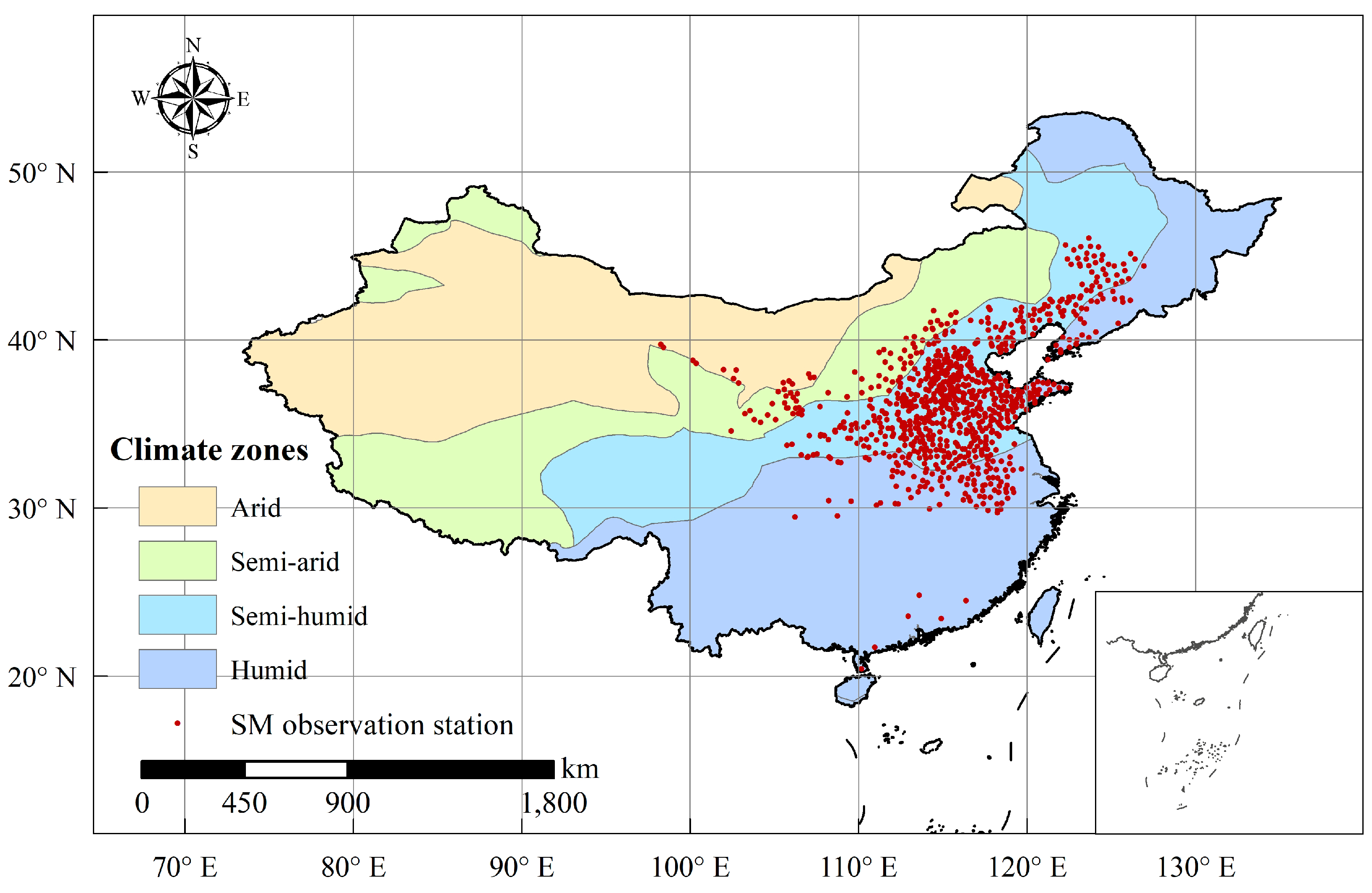
2.1. Study Area and In Situ Monitoring Network

The in situ soil moisture-monitoring network is located in China, as shown in Figure 1. China’s extensive territory spans multiple climate zones. The four climate zones are classified according to annual average precipitation (P) levels from northwest to southeast, the arid zone (P < 200 mm), semi-arid zone (200 mm < P < 400 mm), semi-humid zone (400 mm < P < 800 mm), and humid zone (P > 800 mm). There were 845 monitoring measurements in total. The station numbers in the arid, semi-arid, semi-humid, and humid zones are 14, 66, 593, and 172, respectively. Most stations are located in the semi-humid and humid zones, with relatively fewer stations in the arid and semi-arid zones.

2.2. Data Source

The datasets of SM monitoring were obtained from the Information Center of the Ministry of Water Resources of the People’s Republic of China [24]. Soil moisture was determined using the weighting method after drying. Soil samples were collected manually from four different depths below the surface layer at each monitoring point, which were then dried, cooled, and weighed. The frequency of monitoring was three times per month, or once every ten days. Soil moisture was obtained for four layers: 0–10 cm (1st layer), 10–20 cm (2nd layer), 20–30 cm (3rd layer), and 30–40 cm (4th layer). The obtained soil water represents the moisture weight percentage, which is the weight of soil water in 100 g of soil, and the data unit is g/100 g. The data were collected from 2006 to 2017, but there were limited data in the early stages and many gaps. To ensure consistency and continuity, the data from January 2012 to December 2017 were selected and analyzed in this paper.

The MOD15A2H LAI [27] was downloaded from the Moderate Resolution Imaging Spectroradiometer (MODIS), which was retrieved every 8 days ranging from 2011 to 2018 with a 500 m spatial resolution. The LAI can effectively represent vegetation growth dynamics. Remote sensing LAI monitoring occurred every 8 days, but it may be affected by weather and cloud cover, which can cause errors in the results. The monthly maximum composite method was applied to reduce errors and smooth the data, because the rate of vegetation change is relatively slow.

The meteorological data were collected from the China Meteorological Data Network (http://data.cma.cn), including precipitation (P), air temperature (T), relative humidity (Hum), and sunshine duration (SD) for a daily scale. The four climate zones were classified and extracted based on the levels of annual precipitation. The time series of meteorological and vegetation data are from both 2011 to 2018. To analyze the reason for SM variation, the actual evapotranspiration data, called PML-V2, were obtained from [28]. The temporal resolution was 8 days, and the spatial resolution was 0.05°, which was unified to a monthly scale during 2012–2017.

Teleconnection is the correlation between long-range atmospheric circulation changes, which can reflect the interaction between the ocean and atmospheric circulation. It indicates the impact on the frequency and intensity of extreme climate events, resulting in climate anomalies, and affects hydrological, ecological, and other processes. Four teleconnection indices were selected to analyze the relationship among climate, vegetation, and soil moisture, the El Niño–Southern Oscillation (ENSO), Arctic Oscillation (AO), North Atlantic Oscillation (NAO), and Antarctic Oscillation (AAO). These indices were collected from the National Climate Center of China at a monthly scale.

2.3. Methodology

2.3.1. Pre-Processing and Quality Control of In Situ Monitoring SM Dataset

The monitoring time of SM varied among sites. The frequency of SM monitoring was fixed, that is three times a month. However, the SM data often had missing measurements due to various natural or human factors, resulting in different data volumes at different sites. Even for the same site, the amount of layered SM data at different depths may not be the same. It was necessary to preprocess and control the quality of the data. Firstly, the spatial distribution, data volume, and time pairing information were the effective statistics for the sites for the 1st, 2nd, 3rd, and 4th soil layers, respectively. To match the grid LAI data/meteorological data with the ground observation SM datasets at the same scale, all datasets were downscaled to the point scale. As a widely used downscaling method at the point scale, inverse distance weighting (IDW) is easy to implement with high efficiency [24]. Thereby, the LAI and meteorological data were interpolated to the SM stations by the IDW method, as shown in the following formula.

$$\widehat{\phi }(x_i,y_i)={\displaystyle {\sum }_{j=1}^{nn}\frac{1/{\omega }_j\times {\phi }_j}{{\displaystyle {\sum }_{j=1}^{nn}(1/{\omega }_j})}}$$

(1)

where

• $\widehat{\phi }(x_i,y_i)$—the meteorological or LAI value after adjacent site/grid interpolation;
• ${\phi }_j$—the LAI or meteorological value at the jth neighboring site/grid;
• ${\omega }_j$—the distance between the jth neighboring site/grid and the SM site;
• nn—the number of neighboring sites/grids.

The time dimension information was linked to the spatial data later. The corresponding climate and vegetation data were extracted based on the effective time of the SM data. The resulting data with the same effective time series were used for the subsequent analysis.

2.3.2. Time-Lagged Anomaly Correlation

The temporal responses among climate, vegetation, and soil moisture are calculated in this paper. Specifically, we analyzed how vegetation and soil water respond to climate change, as well as how soil water responds to changes in vegetation. Four climate factors were selected here, precipitation (P), temperature (T), air humid (Hum), and sunshine duration (SD).

The correlation between the LAI or SM and cumulative precipitation, average temperature, average relative air humidity, and cumulative sunshine was analyzed. For the time lag between climate and the LAI, climate factors in the first 0–6 months and the current LAI were used to calculate the correlation. For the time lag between climate and SM, climate factors in the first 0–30 days and the current SM were used to calculate the correlation. The lag response time of vegetation growth and SM dynamics to climate factors in different climatic regions was distinguished based on this.

Meanwhile, the interaction between vegetation growth and soil water is relatively complex. Vegetation evapotranspiration will consume soil water, and the lack of soil water will limit vegetation growth. Therefore, the correlation between soil water in the current month and the vegetation status in the previous 0–6 months and the latter 0–6 months was analyzed. The time-lagged anomaly correlation coefficient rr was used to measure the consistency among the different factors. The calculation formula is as follows.

$$r{r}_{C-LAI}^t={({\displaystyle \sum _{i=1}^n{[(C_i^t-\overline{C_i})(LA{I}_{\mathrm{i}}-\overline{LAI})]}^2}/{\displaystyle \sum _{i=1}^n{(C_i^t-\overline{C_i})}^2{\displaystyle \sum _{i=1}^n{(LA{I}_{\mathrm{i}}-\overline{LAI})}^2}})}^{0.5}$$

(2)

$$r{r}_{C-SM}^t={({\displaystyle \sum _{i=1}^n{[(C_i^t-\overline{C_i})(S{M}_{\mathrm{i}}-\overline{SM})]}^2}/{\displaystyle \sum _{i=1}^n{(C_i^t-\overline{C_i})}^2{\displaystyle \sum _{i=1}^n{(S{M}_{\mathrm{i}}-\overline{SM})}^2}})}^{0.5}$$

(3)

$$r{r}_{SM-LAI}^t={({\displaystyle \sum _{i=1}^n{[(LA{I}_i^t-\overline{LA{I}_i})(S{M}_{\mathrm{i}}-\overline{SM})]}^2}/{\displaystyle \sum _{i=1}^n{(LA{I}_i^t-\overline{LA{I}_i})}^2{\displaystyle \sum _{i=1}^n{(S{M}_{\mathrm{i}}-\overline{SM})}^2}})}^{0.5}$$

(4)

Formulas (2)–(4) show the calculation of the time-lagged anomaly correlation coefficient for climate–vegetation, climate–SM, and vegetation–SM, respectively. Taking Formula (2) as an example, LAI_i is the leaf area at time i. $C_i^t$ means the meteorological condition in the previous t periods. $\overline{C_i}$ and $\overline{LAI}$ refer to the mean value of the series. n means the length of the series. The closer rr approaches 1, the higher the consistency is. If there is a higher rr value in a certain time period, this indicates that this time period is a possible lag time. It is noted that the analysis for the time-lagged anomaly correlation in climate–vegetation, climate–SM, and vegetation–SM was emphasized during the different time periods, which were 0~30 days, 0~6 months, and −6~6 months. To clarify, the anomaly correlation coefficient between the climate lagged n₁ × 1 month (where n₁ ∈ [0,6]) and the LAI was calculated. Similarly, we calculated the anomaly correlation coefficient between climate and the LAI lagged n₂ × 1 day (where n₂ ∈ [0,30]). Additionally, the anomaly correlation coefficients between SM and the LAI for lag and advance n₃ × 1 month (where n₃ ∈ [−6,6]) were also analyzed.

2.3.3. Cross-Wavelet Transform (XWT) Method

The cross-wavelet transform (XWT) is a method used to determine whether a signal exhibits correlation in the time–frequency domain, which can reveal the correlation and time effect in the sequences [29,30]. Therefore, the XWT method was applied to distinguish the impact of teleconnection factors on SM and vegetation dynamics. The cross-wavelet transform between two sets of time series data, An and Bn, is shown as follows.

$$D(\frac{W_{\mathrm{n}}^A(S)W_{\mathrm{n}}^B(S)}{\delta A\delta B}<p)=\frac{Z_{\nu }(p)}{\nu }\sqrt{P_A^k{P}_B^k}$$

(5)

where

• $W_{\mathrm{n}}^A(S)$, $W_{\mathrm{n}}^B(S)$—the continuous wavelet transforms of two time series;
• $P_A^k$, $P_B^k$—the background power spectra;
• $\delta A$, $\delta B$—the standard deviation of An and Bn;
• $Z_{\nu }(p)$—the confidence level of probability p.

3. Results

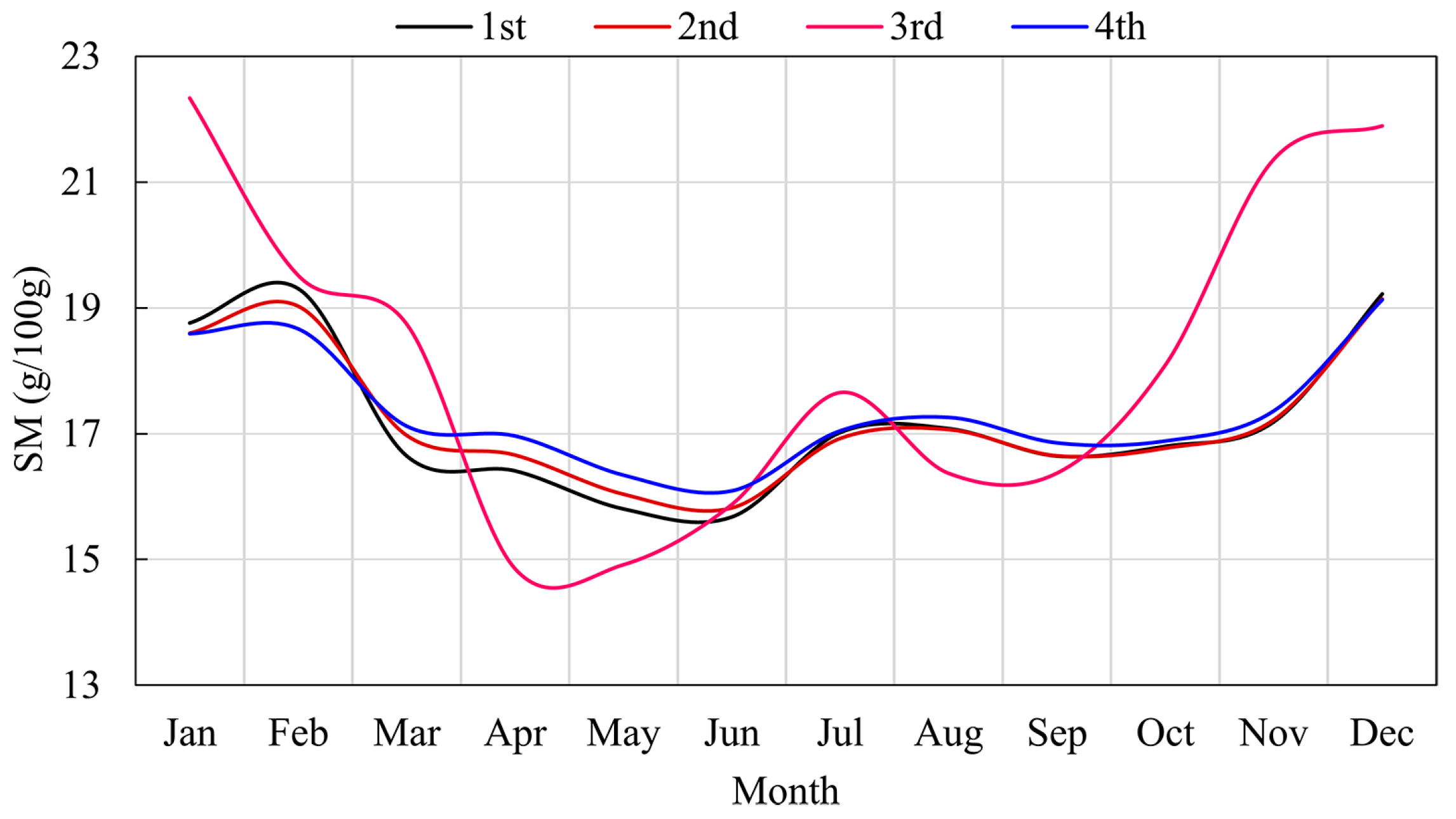
3.1. Spatial Distribution and Temporal Characteristics of Soil Moisture for four Soil Layers

The basic information and distribution of the available SM data is shown in Figure 2. Figure 2a displays the length of the data for each monitoring site, which varied from 1~6 years. The semi-humid and humid areas had the most complete data with the longest sequence. However, there were many missing data in the northeast direction, mainly due to the relative lack of data in the northeast region. Figure 2b shows the average SM values across multiple layers. The color gradient from blue to red indicates an increase in SM from the arid to the humid area or from northwest to southeast, which is consistent with the geographical distribution of the climate zones. The histogram in the bottom-right corner shows that the SM is mostly between 15 and 25 g/100 g, which corresponds to a water content of approximately 15–25 g per 100 g of soil.

The soil moisture at different depths was measured and compared later. The distribution of SM-monitoring measurements and the mean SM of the available data are shown in Figure 2c–f. The amount of SM data is equivalent in the 1st, 2nd, and 4th soil layers. In other words, the determination of soil moisture in the 1st, 2nd, and 4th layers at each site was comprehensive. The SM of the third layer was less frequently measured, with less than 1/8 of the stations reporting data, which were gathered in three main areas: the northwest arid area, the northeast corner of the Bohai Sea, and the southeast of the semi-humid area. The SM at different depths was relatively similar, with higher SM found in deeper soil layers.

Based on the distribution of the climate zones, one site with relatively complete data was selected as a typical site within each zone, and the site locations are shown in

Table 1. Location of the typical stations in the four climate zones.

Climate Zones	Site Name	Longitude	Latitude
Arid zone	Gaoshawo	107.04	37.99
Semi-arid	Mizhi	110.20	37.70
Semi-humid	Lvzhuang	111.25	35.38
Humid	Zhaowan	112.16	33.12

. Then, the dynamic changes in the measured layered soil water were analyzed and are shown in Figure 3. It is important to note that SM measurements in arid areas may be missing due to winter soil freezing. The mean SM gradually increases from arid to humid areas, while from the perspective of the time line, the SM alternates between increasing and decreasing throughout the year. Specifically, the SM increases from January to March, decreases from April to May, reaches its peak from July to August, decreases from September to October, and experiences a slight increase from November to December. Furthermore, the variation trend of the SM at different depths is consistent, with only slight differences in quantity. Generally, changes in surface soil water are more significant than those in the deep layer. This is because surface soil water acts as a link between the atmosphere and the land, resulting in a more direct effect.

It is obvious that the distribution of stations in the semi-humid zone is the densest and most complete, making its data the most representative. For instance, Figure 4 illustrates the annual process of SM change in the semi-humid zone. SM changes exhibit a phased trend throughout the year, increasing from January to February, decreasing from March to May, and increasing again from June to August and September to December. This annual variation is closely linked to precipitation, evapotranspiration, and vegetation growth dynamics. The changes in SM are consistent in the 1st, 2nd, and 4th layers. The amount of data in the third soil layer is relatively small, and they are clustered, so there are certain differences from the changes in SM at other depths; however, the direction and trend of the changes are also consistent. In January-February, the surface soil water is slightly greater than the bottom layer, and then changes the most with time. This indicates that the surface soil is directly influenced by climatic factors as a direct link between the atmosphere and the surface. The effect of precipitation recharge and evapotranspiration consumption is most direct on the surface soil.

3.2. Time Lag and Accumulation Effects among Climate, Vegetation, and Soil Moisture

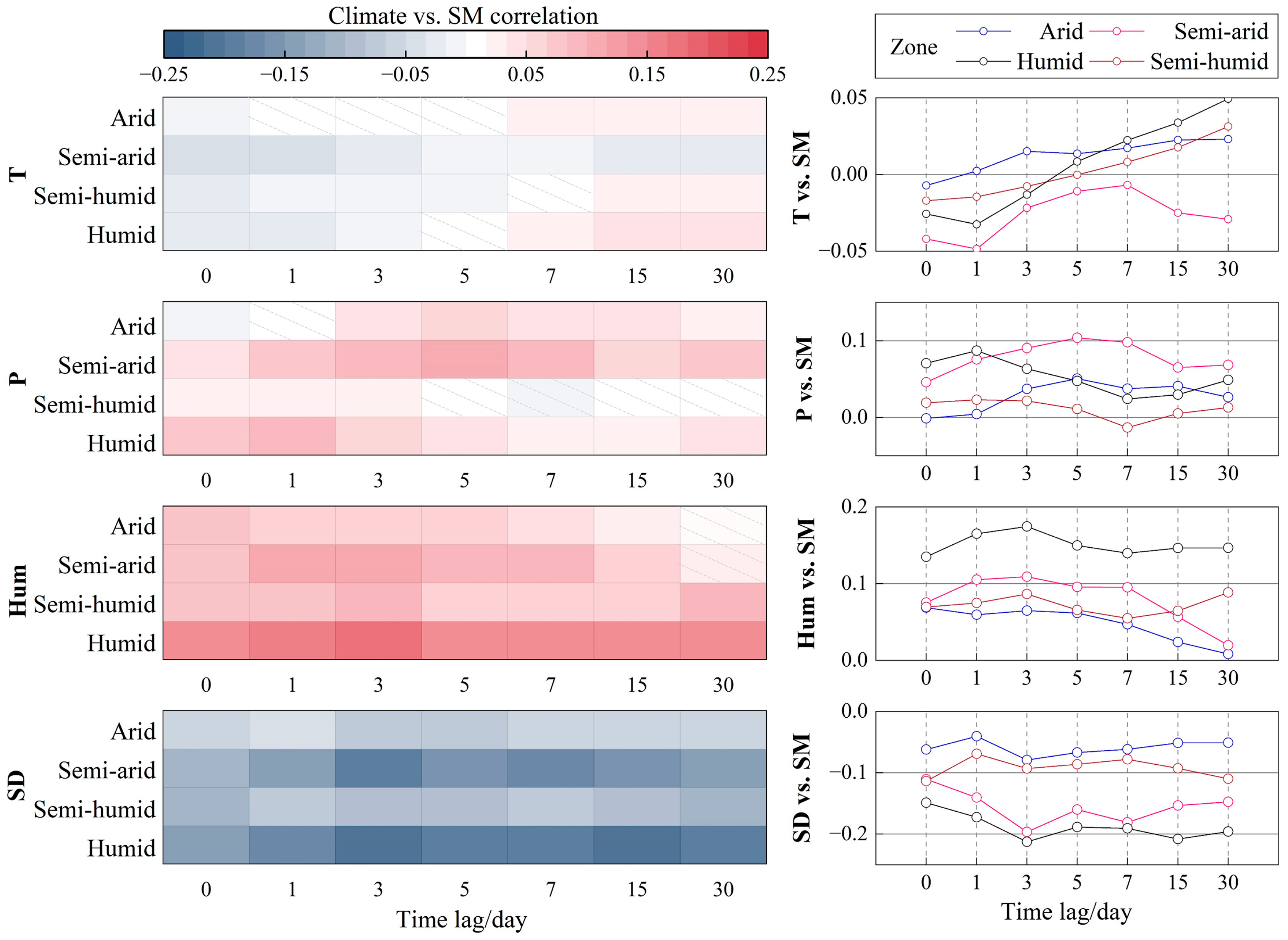
3.2.1. Climate–SM Interaction and Time Lag Effects

It is indicated that changes in SM do not occur simultaneously with changes in climate factors. There appears to be a time lag, as shown in Figure 5. To compare the temporal response of SM dynamics to climate in different climate zones, four climate factors were selected, temperature (T), precipitation (P), relative humidity (Hum), and sunshine hours (SD). The dynamic changes in soil moisture respond to changes in climate factors with a time lag, as shown in Figure 5. This means that early climate conditions will impact soil water. The impact of climate factors on soil water for the first 1, 3, 5, 7, 15, and 30 days was examined to investigate the time delay effect.

T and SD are negatively correlated with SM, while P and Hum are positively correlated. When T is lower in the early stage, SD is shorter, P is higher, and Hum is greater, while SM tends to be higher. The study found that surface soil water is more sensitive to climate factors. This analysis focused on surface soil water as an example. There is a time lag of about 0–3 days between changes in SM and T, and the relationship between them is relatively weak. The time lag between SM and P (Hum or SD) is 3–7 days, 1–3 days, and 3–15 days, respectively. The correlation between SM and P is higher in the arid and semi-arid regions, particularly in the semi-arid region, where water vapor conditions are more sensitive. However, the amount of data in the arid areas is relatively small. It can be observed that semi-arid areas are sensitive to climate change. On the other hand, humid areas are most sensitive to SD, and the accumulated SD in the first 3–15 days will significantly reduce the SM.

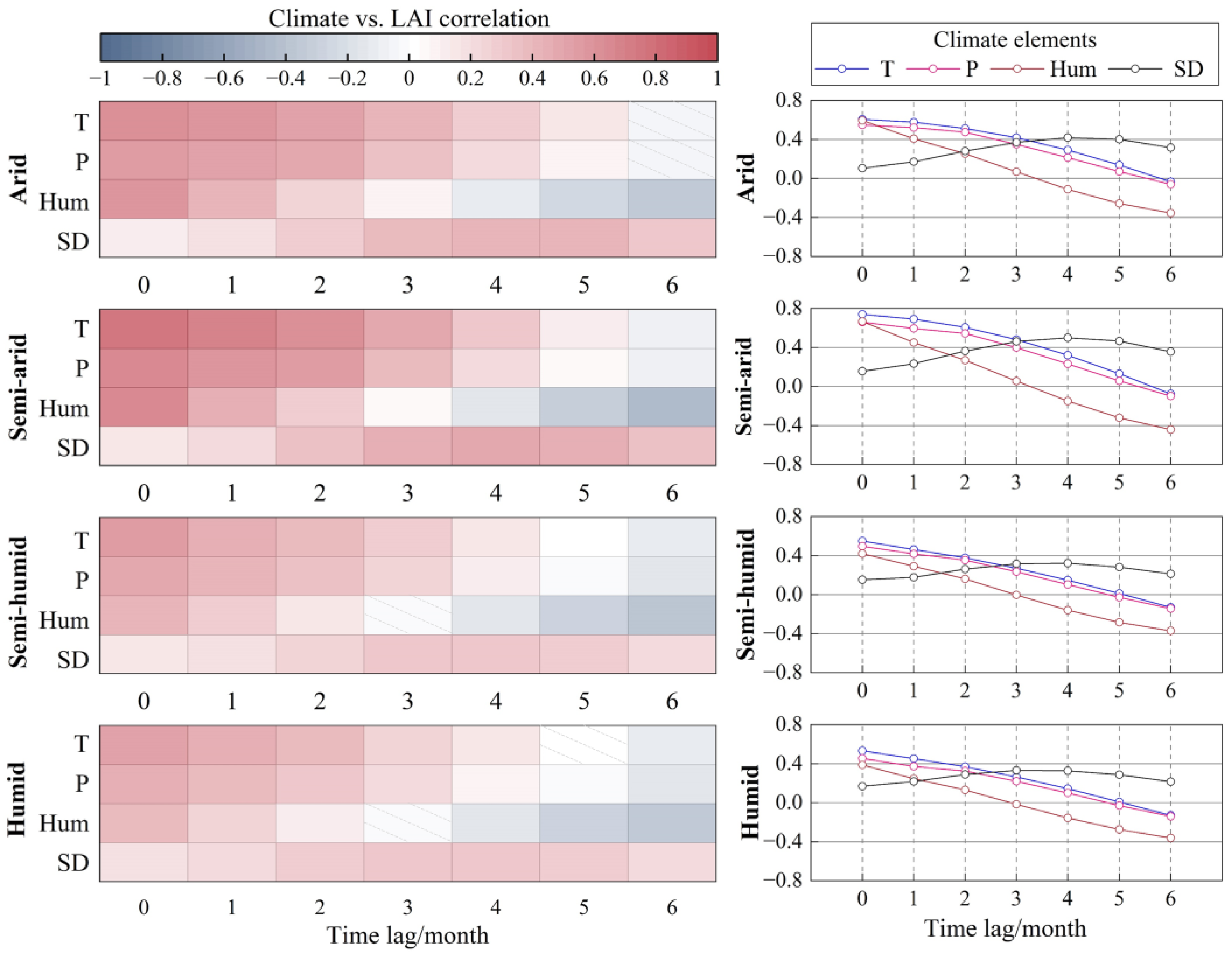
3.2.2. Climate–LAI Interaction and Time Lag Effects throughout Four Climate Zones

Vegetation growth, like SM, responds to climate change with time lag effects. The dynamics of vegetation growth are represented by the leaf area index (LAI). Vegetation growth is a gradual process compared to climate change. This study analyzes the time lag and cumulative effects of climate on vegetation growth on a monthly scale, specifically examining the impact of climate factors in the first 0~6 months on LAI changes (Figure 6). Overall, climate has a positive influence on the LAI. Increasing T, P, SD, and Hum all promote vegetation growth. Vegetation responds quickly to climatic factors, and the LAI is generally highly correlated with climate factors of the current month. Additionally, the vegetation can be affected by the mean T, accumulated P, and mean Hum during the first 1~3 months. However, the T, P, and Hum during the first 4~6 months have little impact on vegetation due to the long time intervals. The impact of SD on vegetation growth is long-lasting, with a lag period of 3~5 months. The cumulative SD during the early stages has a significant effect on vegetation growth. Specifically, the semi-arid region is particularly sensitive to changes in climate factors, with a correlation coefficient greater than 0.65. Vegetation in the arid and semi-arid zones is more sensitive to water constraints, while the humid and semi-humid zones are less constrained by water and more affected by T. This is because humid zones receive relatively sufficient P, and the effect of water is not as significant as in arid zones.

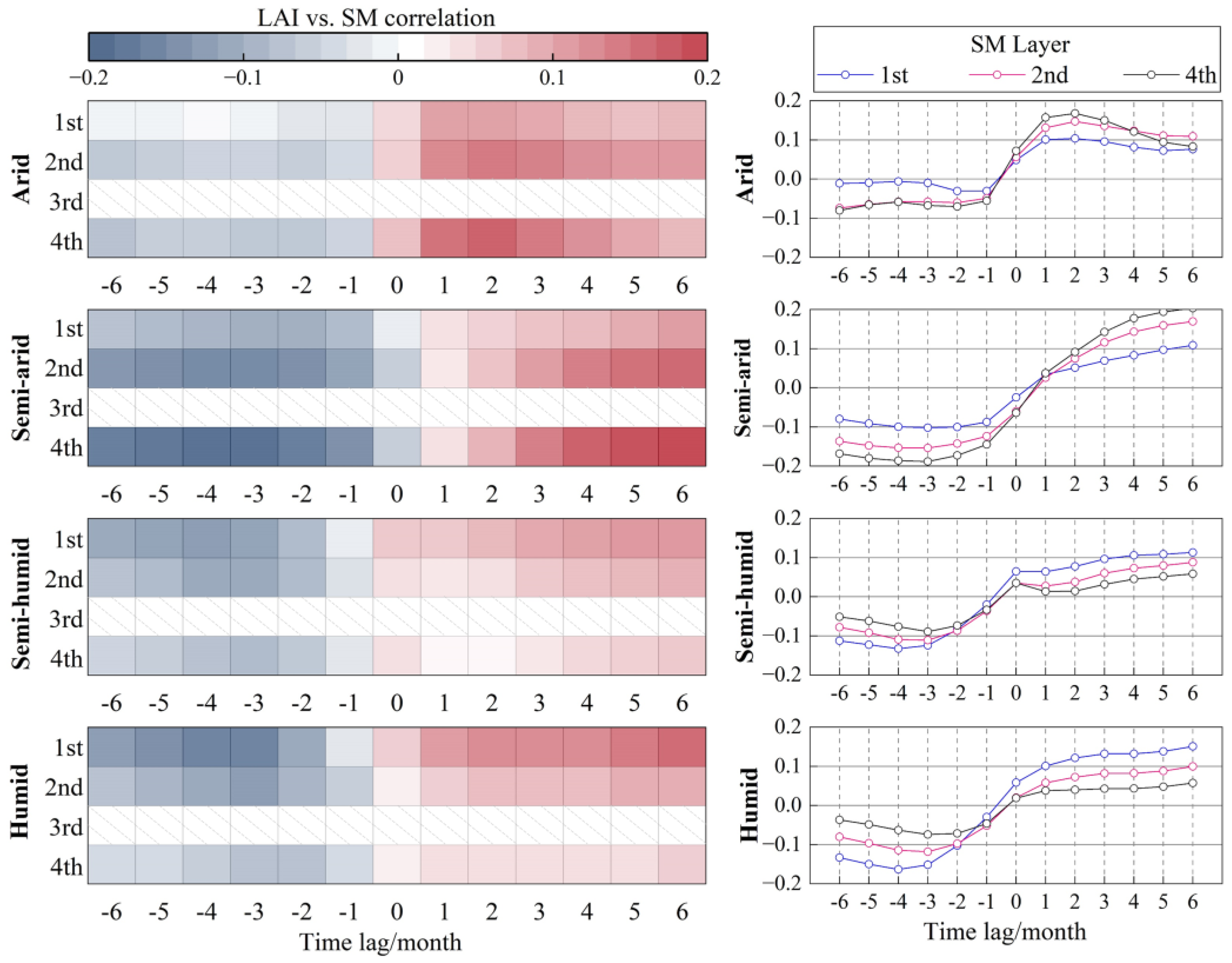
3.2.3. SM–LAI Interaction and Time Lag Effects in Different Layers and Climate Zones

When analyzing the relationship between vegetation and SM, two scenarios were considered: the LAI leading SM (negative on the x-axis) and SM leading the LAI (positive on the x-axis). The dominant role between the LAI and SM was then analyzed, and the results are shown in Figure 7. It is important to note that the analysis was not conducted on the limited data in the third soil layer. The LAI leading SM and SM leading the LAI exhibited contrasting properties. The former exhibited a negative correlation between vegetation and SM (in blue color on the heat map), while the latter exhibited the opposite (in red color). This demonstrates that vegetation growth accelerates evapotranspiration (ET) and reduces SM, while moister soil can promote subsequent vegetation growth.

In the arid and semi-arid zones, the LAI lagged SM with the highest correlation. Vegetation dynamics showed the strongest response to SM changes. The lag in the arid zone was most pronounced for 1~2 months. There were relatively little data for the arid zone, mainly manifested as the LAI lagging SM with a lag time of about 0~2 months. This means that SM in the first two months will constrain vegetation growth, and an increase in soil water will accelerate vegetation growth. In the semi-arid areas, when the LAI led SM, the lead time was about 2–4 months, meaning that vegetation growth affects SM changes, and vegetation growth in the first 2–4 months will affect SM. When SM led the LAI, SM in the first 3–6 months had a positive effect on vegetation growth. The LAI in the humid and semi-humid zones had the strongest correlation with SM, and showed a negative correlation, indicating that vegetation growth in the early stage will inhibit the increase in SM. This leading effect was most evident during the first 2~4 months. Meanwhile, SM also had a promoting effect on secondary vegetation.

Furthermore, the interaction between vegetation and soil in the arid and semi-arid zones was more pronounced in the deep soil layer, which was attributed to the dominant position of deep-rooted vegetation. Conversely, in the semi-humid and humid zones, this interaction was more evident in the surface layer. It is worth noting that the influence of deep soil water on the LAI or vice versa was minimal, and vegetation and soil water were coupled in the shallow layer. This indicates that the root depth of vegetation is greater in the north than in the south [31]. Li et al. [32] described a significant increase in root depth after vegetation restoration in the Loess Plateau region of northern China, thus the response relationship of SM to vegetation dynamics at different depths in different climate zones, which is consistent with research [33].

3.3. Impacts of Teleconnection Factors on Vegetation and Soil Moisture

3.3.1. Dynamic Relation between Teleconnection Factors and LAI

In the field of climate change and research on its response, it is recognized that changes in global ocean temperature or large-scale climate factors may play a crucial role in interdecadal climate, vegetation, and hydrology, such as the ENSO, NAO, AO, etc. [34,35]. Accordingly, correlations between the LAI and the four climatic factors (ENSO, AAO, AO, NAO) are studied through cross-wavelet transform analysis. The correlation between four teleconnection factors and the LAI in different climate zones is shown in

Table 2. Rank correlation coefficient between 4 seasonal teleconnection factors and the LAI.

Climate Zone	Indices	Spring	Summer	Autumn	Winter	Mean
Arid	NAO	/	−0.314	−0.297	−0.397	−0.255
	AO	/	0.073	−0.054	−0.427 *	−0.138
	AAO	/	0.186	0.308	−0.075	0.221
	ENSO	/	−0.169	−0.039	−0.106	−0.074
Semi-arid	NAO	0.231	−0.293	−0.152	−0.325	−0.242
	AO	0.013	0.158	−0.064	−0.539 **	−0.166
	AAO	0.104	0.132	0.159	−0.009	0.208
	ENSO	−0.053	−0.111	−0.071	−0.189	−0.069
Semi-humid	NAO	0.141	−0.175	−0.312	−0.353	−0.223
	AO	0.043	0.038	−0.080	−0.546 **	−0.174
	AAO	0.293	0.274	0.206	−0.053	0.260
	ENSO	0.023	0.011	0.072	−0.099	−0.044
Humid	NAO	−0.034	−0.170	−0.315	−0.424 *	−0.254
	AO	−0.019	0.156	−0.106	−0.528 **	−0.198
	AAO	0.379	0.175	0.157	0.033	0.266
	ENSO	0.028	−0.011	0.069	0.037	−0.030

Note: Symbol “*” represents that the correlation passes the 95% confidence level test, while “**” represents passing the 99% confidence level test.

. Overall, the NAO and AAO have a significant impact on vegetation, with similar correlations across different climate zones. There is a negative correlation between the NAO and LAI, and a positive correlation between the AAO and LAI. The NAO has the greatest impact in the arid and semi-arid zones, and its correlation is highest in winter and summer. The AAO has the greatest impact in the semi-humid and humid zones, and its correlation is highest in spring and summer. The AO has a certain impact on the LAI in humid areas, while the ENSO is negatively correlated with summer vegetation in the arid and semi-arid zones.

Figure 8 shows the various temporal correlation between the LAI and large-scale climate factors. The effective spectral value area is located inside the influence cone curve in the cross-wavelet relationship graph. Arrows indicate phase differences, with the right direction indicating the same phase of the time series and the left direction indicating the opposite [36]. The arrows pointing from left to right indicate that the LAI is in phase with the change in the climate index, and the arrows pointing from right to left indicate the negative phase. If the arrow is pointing upwards, it indicates that the climate factor is three months behind the LAI change, and vice versa, it indicates a three-month-ahead change. The part highlighted by black and bold lines is the confidence interval (significance level of 95%). The redder the color, the higher the correlation is. Taking the NAO and AAO as examples, Figure 8a shows that the effect of the NAO on the LAI was mainly on the scale of 8–16 months. The negative correlation between the NAO and the LAI was mainly reflected on the main scale of 8–16 months in the whole period and on the additional scale of 5–7 months in 2013–2014 and 2015–2016. The main cycle was similar across different climate regions, with minor variations in the sub-cycles. Figure 8l shows that the positive effect of the AAO on the LAI was mainly on the scale of 8–16 months during the whole period, while there was a sub-scale of 0–4 months in 2016–2017 with a lower correlation.

3.3.2. Response in SM Dynamics to Large-Scale Climatic Factors

Similarly, the relationship between layered soil water and large-scale climate factors was also examined, and the results are shown in

Table 3. Rank correlation coefficient between 4 teleconnection factors and SM in different climate zones and SM layers.

SM	Zone	NAO	AO	AAO	ENSO
1st	Arid	0.280 *	−0.115	−0.099	0.470 **
	Semi-arid	0.208 *	0.109	−0.175	0.061
	Semi-humid	0.233 *	0.234 *	−0.136	−0.033
	Humid	0.115	0.119	−0.024	0.145
2nd	Arid	0.401 **	−0.031	−0.130	0.566 **
	Semi-arid	0.154	0.168	−0.197	0.101
	Semi-humid	0.257 **	0.210 *	−0.122	0.028
	Humid	0.156	0.164	−0.014	0.176
4th	Arid	0.101	−0.188	−0.127	0.584 **
	Semi-arid	0.059	0.185	−0.197	0.251 **
	Semi-humid	0.244 **	0.161	−0.124	0.088
	Humid	0.145	0.166	−0.014	0.193

Note: Symbol “*” represents that the correlation passes the 95% confidence level test, while “**” represents passing the 99% confidence level test.

. The results indicate that the ENSO and NAO have the most significant impact on soil water in the arid and semi-arid zones. Meanwhile, the NAO and AO have a greater effect on semi-humid and humid zones. The properties exhibited by different soil layers were similar. Especially in the arid zone, the impact of the ENSO on soil moisture increased with soil depth. However, the data for the third soil layer were insufficient, so they will not be discussed here.

The relationship between the four teleconnection factors and layered SM dynamics was plotted using the cross-wavelet transform method, and the results are shown in Figure 9. Figure 9a illustrates a positive main cycle of approximately 9~15 months between SM and the NAO from 2015 to 2017, and SM changes occurring before the NAO. There is a positive cycle of approximately 9~14 months between SM and the ENSO from 2015 to 2016, and a cycle of 5~10 months in 2013~2014, with SM lagging behind the ENSO, as shown in Figure 9i. At different soil depths, SM displays similar characteristics for the same climate factors from a horizontal perspective. The main cycles are consistent, but there are slight differences in the time series.

4. Discussion

4.1. Annual Variation of SM and Main Driving Factors

SM displayed seasonal variations over time, which were primarily caused by the seasonal changes in climate and vegetation growth in the study area [37]. To determine the annual variation patterns and mechanisms of SM, we conducted a statistical analysis of the annual distribution and changes of precipitation (P), evapotranspiration (ET), and temperature (T) in various climate zones from the soil water stations, as depicted in Figure 10 and Figure 11. The time periods of the P, T, and ET series were all 2012–2017 here, which were consistent with the SM data and counted as the monthly mean value to analyze the seasonal variations. P, T, and ET exhibited a unimodal pattern throughout the year, with their peak occurring in July. Taking the semi-humid zone as an example (Figure 11c), P increased gradually from January to March. In March, T began to rise quickly, and the vegetation growth stage started (March–May). ET also increased rapidly, but P was insufficient to compensate for it (P-ET < 0). Therefore, it can be inferred that SM will increase in spring and early summer, followed by a decrease. Afterwards, P reached a peak during the rainy season and monsoon. At this time, although ET also increased, the amount of P replenishment was greater than the amount of ET (P-ET > 0), so SM began to increase again from July to September. After September, P, T, and ET all decreased rapidly (P-ET > 0), while SM continued to increase. This trend in SM changes throughout the year was consistent with the analysis results of the in situ monitoring measurements, as illustrated in Figure 4. The annual variation was consistent with [24,38]. The trend of SM change in the other three climate zones was similar to that in the semi-humid zone, but the degree of change varied.

4.2. Interaction Effects between Vegetation and Soil Moisture Dynamics

Generally, climate influences both vegetation and SM, generating different response relationships. It is important to note the interaction effect between these two factors [17]. Vegetation growth is a gradual process that depends on specific water and heat conditions, which require not only instantaneous water and heat, but also energy accumulation over periods. As a result, there is a lag and accumulation effect between climate and vegetation [39,40]. Vegetation responds quickly to climatic factors, which is highly correlated with the climate factors of the current month. Moreover, the vegetation can be affected by the mean T, accumulated P, and mean Hum during the first 1~3 months, as shown in Figure 6. The impact of SD on the LAI is longer-lasting, with a lag time of 3~5 months. This is because accumulated sunlight plays a crucial role in the photosynthesis of vegetation growth. The time lag between the Normalized Vegetation Index (NDVI) and climate factors such as T, P, and solar radiation has been analyzed on a global scale [15]. This indicated that the time lag in different zones is about 0~3 months, which is related to longitude and latitude, vegetation type, etc. It has also been pointed out that the impact of climate on vegetation coverage mainly manifests as a lag effect of 0 months and an accumulation effect of 1–2 months [41], which is consistent with the results in this paper. Semi-arid regions are particularly sensitive to climate changes (Figure 6). Vegetation in arid and semi-arid zones is more sensitive to water constraints, while humid and semi-humid zones are more affected by T, because the precipitation in humid areas is sufficient (Figure 11d).

SM is a crucial factor in terrestrial ecosystems. Figure 5 shows that the correlation between SM and P is higher in the arid and semi-arid zones, while the humid zone is the most sensitive to SD. In the arid and semi-arid regions, this correlation is relatively higher, particularly in the semi-arid region, where soil moisture is more sensitive to water vapor conditions. Especially, climate change has a significant impact on the semi-arid region. As mentioned above, an interaction between soil moisture and vegetation exists. For example, favorable climatic conditions (from dry to humid) can stimulate vegetation growth, but SM depletion caused by increased vegetation cover due to warming may lead to further drought [42]. It is important to maintain a balance between vegetation growth and SM dynamics to ensure the sustainability of terrestrial ecosystems. The response between vegetation and SM depends on factors such as climate, vegetation types, and the geographical environment. It was demonstrated that the LAI is positively correlated with SM, with the highest correlation observed when the LAI lags behind SM [18]. Vegetation dynamics exhibit the strongest response to changes in SM. These findings are consistent with the results presented in this paper, as shown in Figure 7. This indicates that SM has a greater impact on secondary vegetation than early vegetation has on SM. As for the response of SM at different depths to climate and vegetation, it is generally observed that surface SM is more sensitive to climate change. Figure 7 shows that the effect of vegetation and deeper SM was significant in the north of China, while they were coupled with shallow SM in the south. The sensitivity of SM to the dynamic response of vegetation is related to the depth of plant roots. It is important to clarify whether deep-rooted or shallow-rooted plants play a leading role [14]. The depth of plant roots in shallow or deep layers is crucial [43]. It has been shown that the root depth of vegetation in northern China significantly increases during vegetation restoration, thereby having a significant impact on deeper SM [31,32].

It is important to acknowledge that ecological protection and vegetation restoration projects are receiving increasing attention with an expanding impact trend. The interactive relationship makes SM a crucial limiting factor for vegetation restoration. A previous study has suggested that afforestation may consume more water in China, where available SM is the key limiting resource [44]. Therefore, soil drying cannot be ignored solely by considering vegetation restoration. How to balance vegetation and SM is an important research direction in the future, and more detailed work is needed.

4.3. Limitations and Uncertainty Analysis

The in situ SM-monitoring network was applied to analyze the time lag and accumulation effects among climate, SM, and vegetation. The quality of the ground-measured soil moisture is important. The in situ monitoring station method used is currently recognized as the most accurate and reliable drying and weighing method. The quality control method adopted is when the soil water content is below 5%; the allowable difference between the three parallel samples monitored at each station was no more than 1%; when the soil water content exceeded 40%, the allowable difference between the three parallel samples monitored at each station was no more than 2%. Although some quality control has been carried out during the measurement process, there are still some shortcomings, such as the following aspects:

(1)

Observation errors: This refers to the data errors caused by the subjective factors of manual operation or objective monitoring equipment.

(2)

Data continuity: Collecting soil data in winter can be challenging due to low temperatures in the north and the impact of soil freezing. As a result, many stations lack observation data during this season.

(3)

Spatial consistency: Achieving consistency in the integrated data from each manual monitoring site is challenging due to variations in operation and management methods across different departments and practical units.

(4)

Impact of agriculture: The location of monitoring stations, particularly in the semi-arid and semi-humid zones, is crucial for agricultural production in China. Agricultural irrigation, which has not been accounted for in this study, may have impacted the SM dynamics. Future analysis could be conducted to investigate this.

(5)

Layered soil data: The datasets consist of SM measurements at depths of 0–40 cm. However, there is a lack of data for the third layer and no monitoring data for deeper SM. Matching the distribution of root depth would improve the analysis of the dynamic relationship between vegetation and SM. Deep SM-monitoring networks or estimating methods for the root–surface relationship can be improved in the future [45,46].

(6)

SM observation stations can monitor soil water dynamics at a single point, but their representativeness is limited due to the spatial heterogeneity of underlying factors [47]. In the future, the quality of SM data products can be improved by combining remote sensing detection technology, scale conversion methods, and data fusion technology [48]. This will provide new impetus for exploring hydrological processes in river basins.

5. Conclusions

The response of vegetation and SM to climate change was analyzed, as well as the complex relationship between vegetation and SM dynamics, using data from over 800 in situ SM-monitoring measurements in China. Additionally, the time effects of various large-scale teleconnection factors on vegetation and SM were analyzed by using the cross-wavelet transform method. The findings are listed as follows:

(1)

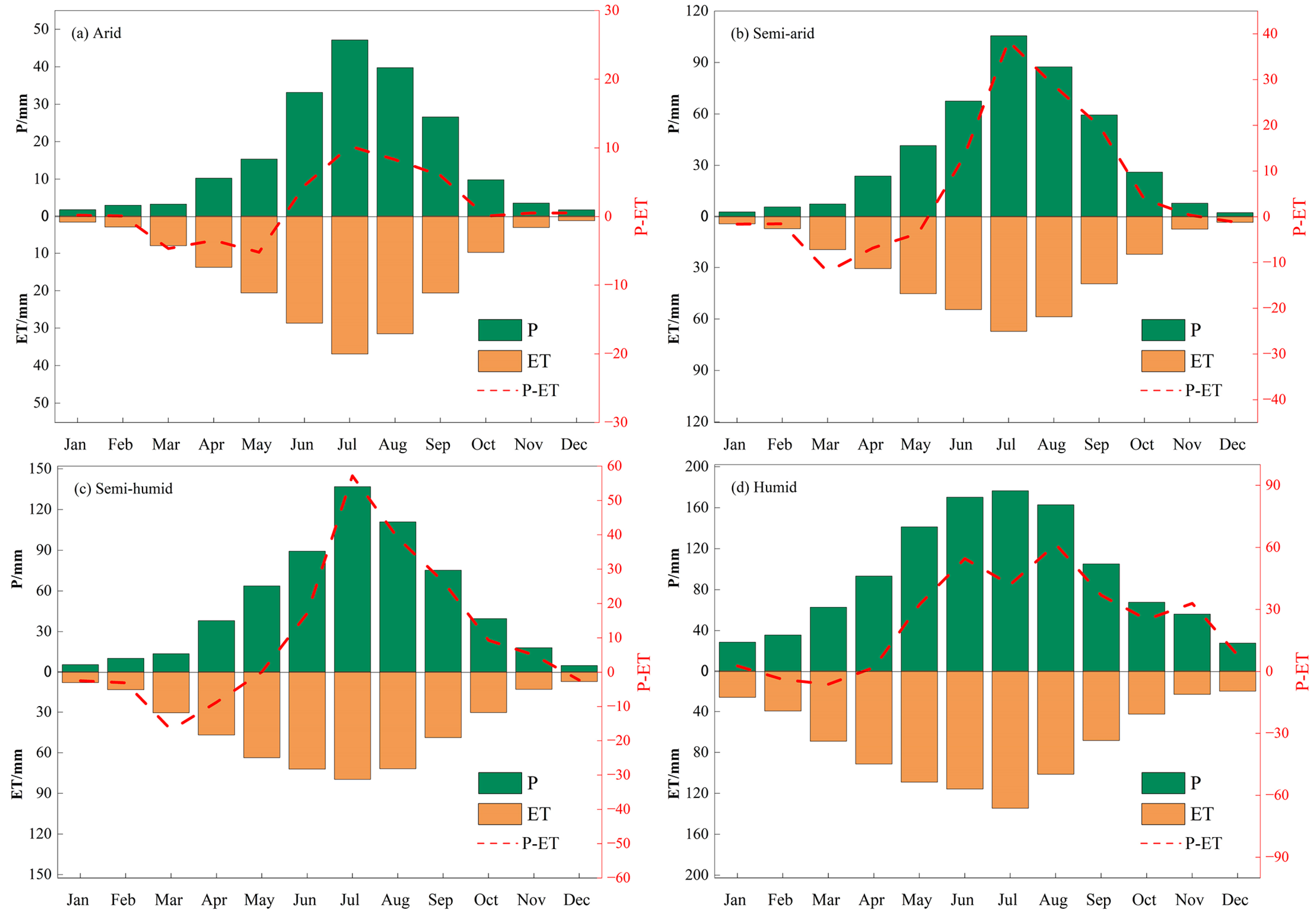
In China, SM tends to become wetter from northwest to southeast, with a water weight of approximately 15–25 g per 100 g of soil. The surface SM exhibits the greatest variation. The annual variation of SM follows a phased change pattern in response to P, T, and vegetation growth.

(2)

The response of surface SM to climate change is most sensitive. SM is negatively correlated with T and SD, while it is positively correlated with P and Hum. The response time of SM to climate factors varies. SM is more sensitive to water vapor conditions in the arid zone, while the humid zone is most sensitive to heat quantity.

(3)

The relationships for the LAI leading SM (negative correlation) and SM leading the LAI (positive correlation) exhibit opposite properties. This is more significant in the arid and semi-arid zones, with a response time of 2~4 months between the LAI and SM. The interaction between the LAI and SM is more pronounced in deep layers in the arid zone, while it is more pronounced in surface layers in humid areas, which is related to the depth distribution of vegetation roots.

(4)

The NAO has the greatest impact on the LAI in the arid and semi-arid zones (mainly in winter and summer), while the AAO does in the semi-humid and humid zones (in spring and summer). There is a main influence period for about 8–16 months between teleconnection factors and the LAI. The NAO and AO have a greater impact on SM in the humid region, while the ENSO and NAO do on SM in the arid zone.

The results are useful for supporting ecological restoration and future water resource management and enhancing the carrying capacity and resilience of China.

References

1. Bowen, G. The diversified economics of soil water. Nature 2015, 525, 43–44. [Google Scholar] [CrossRef]
2. Vereecken, H.; Amelung, W.; Bauke, S.; Bogena, H.; Brüggemann, N.; Montzka, C.; Vanderborght, J.; Bechtold, M.; Blöschl, G.; Carminati, A.; et al. Soil hydrology in the Earth system. Nat. Rev. Earth Environ. 2022, 3, 573–587. [Google Scholar] [CrossRef]
3. Dong, J.; Akbar, R.; Gianotti, D.; Feldman, A.; Crow, W.; Entekhabi, D. Can Surface Soil Moisture Information Identify Evapotranspiration Regime Transitions? Geophys. Res. Lett. 2022, 49, e2021GL097697. [Google Scholar] [CrossRef]
4. Zhu, L.; Yang, M.; Liu, J.; Zhang, Y.; Chen, X.; Zhou, B. Evolution of the freeze-thaw cycles in the source region of the Yellow River under the influence of climate change and its hydrological effects. J. Ground. Sci. Eng. 2022, 10, 322–334. [Google Scholar]
5. Guan, Y.; Gu, X.; Slater, L.; Li, J.; Kong, D.; Zhang, X. Spatio-temporal variations in global surface soil moisture based on multiple datasets: Intercomparison and climate drivers. J. Hydrol. 2023, 625, 130095. [Google Scholar] [CrossRef]
6. Liu, Z.; Notaro, M.; Gallimore, R. Indirect vegetation-soil moisture feedback with application to Holocene North Africa climate. Glob. Change Biol. 2010, 16, 1733–1743. [Google Scholar] [CrossRef]
7. Nigenare, A.; Meng, Y.; Wang, J.; Ge, X.; Tang, Z. Climate overtakes vegetation greening in regulating spatiotemporal patterns of soil moisture in arid Central Asia in recent 35 years. GISci. Remote Sens. 2024, 61, 2286744. [Google Scholar] [CrossRef]
8. Zhu, Z.; Piao, S.; Myneni, R.; Huang, M.; Zeng, Z.; Canadell, J.; Ciais, P.; Sitch, S.; Friedlingstein, P.; Arneth, A. Greening of the Earth and its drivers. Nat. Clim. Change 2016, 6, 791. [Google Scholar] [CrossRef]
9. Qin, G.; Meng, Z.; Fu, Y. Drought and water-use efficiency are dominant environmental factors affecting greenness in the Yellow River Basin, China. Sci. Total Environ. 2022, 834, 155479. [Google Scholar] [CrossRef]
10. Wang, C.; Chen, J.; Gu, L.; Wu, G.; Tong, S.; Xiong, L.; Xu, C. A pathway analysis method for quantifying the contributions of precipitation and potential evapotranspiration anomalies to soil moisture drought. J. Hydrol. 2023, 621, 129570. [Google Scholar] [CrossRef]
11. Romano, N. Soil moisture at local scale: Measurements and simulations. J. Hydrol. 2014, 516, 6–20. [Google Scholar] [CrossRef]
12. Han, Z.; Huang, Q.; Huang, S.; Leng, G.; Bai, Q.; Liang, H.; Wang, L.; Zhao, J.; Fang, W. Spatial-temporal dynamics of agricultural drought in the Loess Plateau under a changing environment: Characteristics and potential influencing factors. Agric. Water Manag. 2021, 244, 106540. [Google Scholar] [CrossRef]
13. Li, W.; Wang, Y.; Yang, J.; Deng, Y. Time-Lag Effect of Vegetation Response to Volumetric Soil Water Content: A Case Study of Guangdong Province, Southern China. Remote Sens. 2022, 14, 1301. [Google Scholar] [CrossRef]
14. Li, S.; Sawada, Y. Soil moisture-vegetation interaction from near-global in-situ soil moisture measurements. Environ. Res. Lett. 2022, 17, 114028. [Google Scholar] [CrossRef]
15. Wu, D.; Zhao, X.; Liang, S.; Zhou, T.; Huang, K.; Tang, B.; Zhao, W. Time-lag effects of global vegetation responses to climate change. Glob. Change Biol. 2015, 21, 3520–3531. [Google Scholar] [CrossRef]
16. Xu, S.; Wang, Y.; Liu, Y.; Li, J.; Qian, K.; Yang, X.; Ma, X. Evaluating the cumulative and time-lag effects of vegetation response to drought in Central Asia under changing environments. J. Hydrol. 2023, 627, 130455. [Google Scholar] [CrossRef]
17. Yu, T.; Bao, A.; Zhang, J.; Tu, H.; Chen, B.; De Maeyer, P.; Van de Voorde, T. Evaluating surface soil moisture characteristics and the performance of remote sensing and analytical products in Central Asia. J. Hydrol. 2023, 617, 128921. [Google Scholar] [CrossRef]
18. Xu, L.; Gao, G.; Wang, X.; Fu, B. Distinguishing the effects of climate change and vegetation greening on soil moisture variability along aridity gradient in the drylands of northern China. Agric. For. Meteorol. 2023, 343, 109786. [Google Scholar] [CrossRef]
19. Kong, D.; Miao, C.; Wu, J.; Zheng, H.; Wu, S. Time lag of vegetation growth on the Loess Plateau in response to climate factors: Estimation, distribution, and influence. Sci. Total Environ. 2020, 744, 140726. [Google Scholar] [CrossRef]
20. Feng, Y.; Wang, H.; Liu, W.; Sun, F. Global Soil Moisture-Climate Interactions during the Peak Growing Season. J. Clim. 2023, 36, 1187–1196. [Google Scholar] [CrossRef]
21. Konkathi, P.; Karthikeyan, L. Utility of L-band and X-band vegetation optical depth to examine vegetation response to soil moisture droughts in South Asia. Remote Sens. Environ. 2023, 301, 113933. [Google Scholar] [CrossRef]
22. Babaeian, E.; Sadeghi, M.; Jones, S.; Montzka, C.; Vereecken, H.; Tuller, M. Ground, Proximal, and Satellite Remote Sensing of Soil Moisture. Rev. Geophys. 2019, 57, 530–616. [Google Scholar] [CrossRef]
23. Stillman, S.; Zeng, X. Evaluation of SMAP Soil Moisture Relative to Five Other Satellite Products Using the Climate Reference Network Measurements Over USA. IEEE Trans. Geosci. Remote Sens. 2018, 56, 6296–6305. [Google Scholar] [CrossRef]
24. Yang, Y.; Zhang, J.; Bao, Z.; Ao, T.; Wang, G.; Wu, H.; Wang, J. Evaluation of multi-source soil moisture datasets over central and eastern agricultural area of China using in situ monitoring network. Remote Sens. 2021, 13, 1175. [Google Scholar] [CrossRef]
25. Chen, C.; Park, T.; Wang, X.; Piao, S.; Xu, B.; Chaturvedi, R.; Fuchs, R.; Brovkin, V.; Ciais, P.; Fensholt, R.; et al. China and India lead in greening of the world through land-use management. Nat. Sustain. 2019, 2, 122–129. [Google Scholar] [CrossRef] [PubMed]
26. Dou, Y.; Tong, X.; Horion, S.; Feng, L.; Fensholt, R.; Shao, Q.; Tian, F. The success of ecological engineering projects on vegetation restoration in China strongly depends on climatic conditions. Sci. Total Environ. 2024, 915, 170041. [Google Scholar] [CrossRef] [PubMed]
27. Ma, L.; Cui, Y.; Liu, B.; Liao, B.; Wei, J.; Han, H.; Tian, W. A GIS-based method for modeling methane emissions from paddy fields by fusing multiple sources of data. Sci. Total Environ. 2022, 859, 159917. [Google Scholar] [CrossRef] [PubMed]
28. Zhang, Y.; Kong, D.; Gan, R.; Chiew, F.; McVicar, T.; Zhang, Q.; Yang, Y. Coupled estimation of 500 m and 8-day resolution global evapotranspiration and gross primary production in 2002–2017. Remote Sens. Environ. 2019, 222, 165–182. [Google Scholar] [CrossRef]
29. Grinsted, A.; Moore, J.; Jevrejeva, S. Application of the cross wavelet transform and wavelet coherence to geophysical time series. Nonlinear Process. Geophys. 2004, 11, 561566. [Google Scholar] [CrossRef]
30. Wang, F.; Lai, H.; Li, Y.; Feng, K.; Tian, Q.; Guo, W.; Qu, Y.; Yang, H. Spatio-temporal evolution and teleconnection factor analysis of groundwater drought based on the GRACE mascon model in the Yellow River Basin. J. Hydrol. 2023, 626, 130349. [Google Scholar] [CrossRef]
31. Hauser, E.; Sullivan, P.; Flores, A.; Hirmas, D.; Billings, S. A Global-scale shifts in rooting depths due to anthropocene land cover changes pose unexamined consequences for critical zone functioning. Earth Future 2022, 10, e2022EF002897. [Google Scholar] [CrossRef]
32. Li, B.; Zhang, W.; Li, S.; Wang, J.; Liu, G.; Xu, M. Severe depletion of available deep soil water induced by revegetation on the arid and semiarid Loess Plateau. For. Ecol. Manag. 2021, 491, 119156. [Google Scholar] [CrossRef]
33. Li, M.; Wu, P.; Ma, Z.; Pan, Z.; Lv, M.; Yang, Q.; Duan, Y. The Increasing Role of Vegetation Transpiration in Soil Moisture Loss across China under Global Warming. J. Hydrometeorol. 2022, 23, 253–274. [Google Scholar] [CrossRef]
34. Dong, L.; Fu, C.; Liu, J.; Zhang, P. Combined Effects of Solar Activity and El Nio on Hydrologic Patterns in the Yoshino River Basin, Japan. Water Resour. Manag. 2018, 32, 2421–2435. [Google Scholar] [CrossRef]
35. Zhao, J.; Huang, S.Z.; Huang, Q. Time-lagged response of vegetation dynamics to climatic and teleconnection factors. Catena 2020, 189, 104474. [Google Scholar] [CrossRef]
36. Lin, Q.; Wu, Z.; Singh, V.; Sadeghi, S.; He, H.; Lu, G. Correlation between hydrological drought, climatic factors, reservoir operation, and vegetation cover in the Xijiang Basin, South China. J. Hydrol. 2017, 549, 512–524. [Google Scholar] [CrossRef]
37. Zwieback, S.; Colliander, A.; Cosh, M.; Martínez-Fernándezj, J.; McNairn, H.; Starks, P.; Thibeault, M.; Berg, A. Estimating time-dependent vegetation biases in the SMAP soil moisture product. Hydrol. Earth Syst. Sci. 2018, 22, 4473–4489. [Google Scholar] [CrossRef]
38. Liu, Y.; Yang, Y. Spatial-temporal variability pattern of multi-depth soil moisture jointly driven by climatic and human factors in China. J. Hydrol. 2023, 619, 129313. [Google Scholar] [CrossRef]
39. Ding, Y.; Li, Z.; Peng, S. Global analysis of time-lag and-accumulation effects of climate on vegetation growth. Int. J. Appl. Earth Obs. 2020, 92, 102179. [Google Scholar] [CrossRef]
40. Wen, Y.; Liu, X.; Xin, Q.; Wu, J.; Xu, X.; Pei, F.; Li, X.; Du, G.; Cai, Y.; Lin, K. Cumulative effects of climatic factors on terrestrial vegetation growth. J. Geophys. Res-Biogeo. 2019, 124, 789–806. [Google Scholar] [CrossRef]
41. Ma, M.; Wang, Q.; Liu, R.; Zhao, Y.; Zhang, D. Effects of climate change and human activities on vegetation coverage change in northern China considering extreme climate and time-lag and -accumulation effects. Sci. Total Environ. 2023, 860, 160527. [Google Scholar] [CrossRef] [PubMed]
42. Deng, Y.; Wang, S.; Bai, X.; Luo, G.; Wu, L.; Chen, F.; Wang, J.; Li, C.; Yang, Y.; Hu, Z.; et al. Vegetation greening intensified soil drying in some semi-arid and arid areas of the world. Agric. For. Meteorol. 2020, 292, 108103. [Google Scholar] [CrossRef]
43. Neill, C.; Coe, M.T.; Riskin, S.H.; Krusche, A.; Elsenbeer, H.; Macedo, M.; McHorney, R.; Lefebvre, P.; Davidson, E.; Scheffler, R.; et al. Watershed responses to Amazon soya bean cropland expansion and intensification. Philos. Trans. R. Soc. B Biol. Sci. 2013, 368, 20120425. [Google Scholar] [CrossRef] [PubMed]
44. Cao, J.; Tian, H.; Adamowski, J.; Zhang, X.; Cao, Z. Influences of afforestation policies on soil moisture content in China’s arid and semi-arid regions. Land Use Policy 2018, 75, 449–458. [Google Scholar] [CrossRef]
45. Yang, Y.; Bao, Z.; Wu, H.; Wu, H.; Wang, G.; Liu, C.; Wang, J.; Zhang, J. An Exponential Filter Model-Based Root-Zone Soil Moisture Estimation Methodology from Multiple Datasets. Remote Sens. 2022, 14, 1785. [Google Scholar] [CrossRef]
46. Baldwin, D.; Manfreda, S.; Keller, K.; Smithwick, E. Predicting root zone soil moisture with soil properties and satellite near-surface moisture data across the conterminous United States. J. Hydrol. 2017, 546, 393–404. [Google Scholar] [CrossRef]
47. Yilmaz, M.; Crow, W.; Anderson, M.; Hain, C. An objective methodology for merging satellite- and model-based soil moisture products. Water Resour. Res. 2012, 48, W11502. [Google Scholar] [CrossRef]
48. Gruber, A.; Scanlon, T.; Schalie, R.; Wagner, W.; Dorigo, W. Evolution of the ESA CCI soil moisture climate data records and their underlying merging methodology. Earth Syst. Sci. Data 2019, 11, 717–739. [Google Scholar] [CrossRef]
Figure 1. Locations of study area and in situ ground soil moisture (SM)-monitoring network, together with the distribution of climate zones. Four climate zones are involved here: arid, semi-arid, semi-humid, humid.
Remotesensing 16 02063 g001
Figure 2. Distribution of available SM data over four soil layers. (a) shows the data duration in each in situ monitoring station represented by the depth of the red color. (bf) show the mean SM value at multiple layers and each soil layer, while the inset bar plot shows the number of sites in different SM categories.
Remotesensing 16 02063 g002
Figure 3. The dynamics of layered SM measured at typical sites in each climate zone.
Remotesensing 16 02063 g003
Figure 4. Seasonality of soil moisture distribution in the semi-humid zone.
Remotesensing 16 02063 g004
Figure 5. Climate–SM correlation in the surface soil layer throughout the four climate zones considering different time lag scenarios presented as heatmaps (left) and string diagrams (right), respectively. A slash symbol in the heat maps indicates the insignificant climate–LAI anomaly correlation with a 95% significance level.
Remotesensing 16 02063 g005
Figure 6. Climate–LAI correlation throughout the four climate zones considering different time lag scenarios presented as heatmaps (left) and string diagrams (right), respectively.
Remotesensing 16 02063 g006
Figure 7. LAI–SM correlation throughout the four climate zones considering different time lag scenarios presented as heatmaps (left) and string diagrams (right), respectively. Note: LAI leading SM—negative horizontal coordinate; SM leading LAI—positive horizontal coordinate.
Remotesensing 16 02063 g007
Figure 8. Cross-wavelet transform diagram between teleconnection factors and the LAI in the four climate zones. (ad) shows cross-wavelet between NAO and LAI in four climate zones. (eh) shows cross-wavelet between AO and LAI. (il) shows cross-wavelet between AAO and LAI. (mp) shows cross-wavelet between ENSO and LAI in four climate zones.
Remotesensing 16 02063 g008
Figure 9. Cross-wavelet transform diagram between teleconnection factors and SM from 3 different depth layers. (ac) shows cross-wavelet between NAO and SM in 3 depth layers. (df) shows cross-wavelet between AO and SM. (gi) shows cross-wavelet between AAO and SM. (jl) shows cross-wavelet between ENSO and SM in 3 depth layers.
Remotesensing 16 02063 g009
Figure 10. Annual variation of temperature over the four climate zones during 2012–2017.
Remotesensing 16 02063 g010
Figure 11. The annual variance of precipitation and evapotranspiration throughout the four climate zones.
Remotesensing 16 02063 g011