Article

Low-Sidelobe Imaging Method Utilizing Improved Spatially Variant Apodization for Forward-Looking Sonar

1
Institute of Acoustics, Chinese Academy of Sciences, Beijing 100190, China
2
College of Underwater Acoustic Engineering, Harbin Engineering University, Harbin 150001, China
*
Author to whom correspondence should be addressed.
Remote Sens. 2024, 16(12), 2100; https://doi.org/10.3390/rs16122100
Submission received: 22 April 2024 / Revised: 28 May 2024 / Accepted: 6 June 2024 / Published: 10 June 2024

Abstract

:
For two-dimensional forward-looking sonar imaging, high sidelobes significantly degrade the quality of sonar images. The cosine window function weighting method is often applied to suppress the sidelobe levels in the angular and range dimensions, at the expense of the main lobe resolutions. Therefore, an improved spatially variant apodization imaging method for forward-looking sonar is proposed, to reduce sidelobes without degrading the main lobe resolution in angular-range dimensions. The proposed method is a nonlinear postprocessing operation in which the raw complex-valued sonar image produced by a conventional beamformer and matched filter is weighted by a spatially variant coefficient. To enhance the robustness of the spatially variant apodization approach, the array magnitude and phase errors are calibrated to prevent the occurrence of beam sidelobe increase prior to beamforming operations. The analyzed results of numerical simulations and a lake experiment demonstrate that the proposed method can greatly reduce the sidelobes to approximately −40 dB, while the main lobe width remains unchanged. Moreover, this method has an extremely simple computational process.

1. Introduction

Imaging sonars can directly present underwater scene information, providing strong support for underwater target detection and recognition [1,2,3]. Imaging sonars can be divided by their detection coverage and system construction type into: forward-looking [4], side-looking [5] and down-looking solutions [6]. In this paper, two-dimensional forward-looking sonar (FLS) is discussed, and a forward-looking sonar imaging method is proposed to reduce sidelobes without sacrificing main lobe resolution.
Generally, for FLS, the angular dimension is obtained via conventional beamforming for a uniform linear array, and the range dimension is obtained via match filtering for a linear frequency modulated signal [7,8]. For the output envelopes of conventional beamforming and match filtering, the main-to-side ratio of both is approximately −13 dB [9,10]. Typically, in practical engineering, the ratio needs to be approximately −40 dB to acquire high-quality sonar images. In practice, high sidelobe levels from a strong target echo can weaken or even completely mask the main lobe of a smaller target echo, so additional sidelobe suppression for FLS images is essential [11,12].
Conventional amplitude weighting cosine window functions are commonly applied to reduce the sidelobe levels with angular and range dimensions for FLSs, which may lead to the degradation of the angular and range resolutions. Compared with conventional beamforming, sonar images are obtained with lower sidelobe levels and narrower main lobe widths by utilizing adaptive beamforming (ADBF) [13,14,15,16]. Nevertheless, the performance of the ADBF methods degrades in the presence of array model mismatch due to imperfect array channels and inaccurately estimated data covariance matrices; hence, several robust adaptive beamforming algorithms have been investigated. The calculation of the adaptive weighed vector in robust adaptive beamforming is equivalent to the second-order cone programming problems, which has high complexity; furthermore, the prior knowledge of the programming problem is difficult to obtain due to complicated underwater propagation [17]. Moreover, for forward-looking imaging sonar, these existing adaptive beamforming approaches are not applicable to the output in the range dimension. Thus, robust adaptive beamforming cannot be easily used to obtain lower sidelobe levels for forward-looking sonar imaging.
Compressive sensing (CS) has been proposed for use in arrays to improve the resolution of the spatial spectrum of underwater source locations in passive sonar. Compressed beamforming has also proven to be an effective approach for improving sonar image quality without increasing the array size [18,19,20,21]. Additionally, a few transducers can be implemented in compressed beamforming to obtain a similar image quality to that produced by a larger-aperture array. Nevertheless, the performance of CS in underwater acoustics imaging will be limited, because prior knowledge cannot be properly matched to the reverberation-rich scenes of underwater environments.
Deconvolution algorithms have been proposed to improve the angular resolution in spatial spectrum estimation by processing beamformer output data. These methods were subsequently extended to high-frequency sonar imaging to achieve higher resolution in both the angular and range dimensions simultaneously [7,8,12,22,23,24,25,26,27]. However, the deconvolution results require several iterations, and the performance is related to the number of iterations. Thus, the application of this method in engineering is hindered by its high computational complexity.
The spatially variant apodization (SVA) method was proposed and applied for synthetic aperture radar (SAR) imaging. In this method, the properties of the cosine-on-pedestal weighing functions are utilized to achieve range dimension sidelobe suppression without broadening the main lobe [28,29,30,31]. Furthermore, it is regarded as a postprocessing method with a lower computational cost in the image domain. Moreover, it can preserve the raw sonar image. However, the principle of SAR imaging is different from that of forward-looking sonar imaging, and the frequency domain characteristics of windows are utilized for the SVA method in the field of SAR imaging. For forward-looking sonar, the multibeams are obtained by beamforming at the sonar system receiving end, and the sidelobes need to be reduced in the beam domain. An image is formed per frame in forward-looking imaging sonar, while an SAR image is generated by platform continuous motion fusion. So, the raw image data properties and image coordinate system of the forward-looking imaging sonar are different from those of SAR. Hence, the SVA method used in SAR cannot be directly applied to imaging sonar sidelobe reduction. Nevertheless, the use of the SVA method has rarely been reported in the forward-looking imaging sonar field, and the original SVA method is less robust to existing array amplitude phase errors. In this paper, we analyze the peculiarities of the beamforming output and matched filter output using cosine window weighting for forward-looking imaging sonar, combined with the SVA method to reduce sidelobes in angular-range dimensions. Additionally, array amplitude phase errors are calibrated to enhance the robustness of the original SVA method.
To obtain lower sidelobe levels without degrading the main lobe resolution in angular-range dimensions, an improved spatially variant apodization forward-looking sonar imaging method is proposed in this article. The proposed method is a nonlinear postprocessing operation in which the raw complex-valued sonar image data produced by a conventional beamformer and matched filter are weighted by a spatially variant coefficient. To enhance the robustness of the spatially variant apodization approach, the array magnitude and phase errors are calibrated to avoid beam sidelobe heightening prior to beamforming operations. The analyzed results of the numerical simulations and a lake experiment demonstrate that the proposed method can greatly reduce the sidelobes to approximately −40 dB while the main lobe width remains unchanged. Moreover, this method uses an extremely simple computational procedure.
The rest of the paper is organized as follows. In Section 2, the conventional forward-looking sonar imaging procedure is described. The improved forward-looking sonar imaging method, which utilizes spatially variant apodization combined with array magnitude and phase error calibration, is described in Section 3. Analyses of the simulation and lake experiment results are presented to demonstrate the effectiveness of the proposed approach in Section 4. In Section 5, the conclusions are provided.

2. Conventional Variant Apodization for Forward-Looking Sonar Imaging

In this section, the signal model of forward-looking imaging sonar is first described. Then, conventional variant apodization methods are introduced.

2.1. Signal Model

We assume that forward-looking imaging sonar is composed of a single transmitter and a receiving uniform linear array (ULA) with N elements at a half-wavelength spacing. For simplicity, the narrowband far-field underwater targets are assumed to be ideal point scatterers. The transmission loss and the medium absorption loss associated with free-space propagation are neglected, and the underwater reverberations and noise are ignored.
For a target, the discrete baseband echo received by the   n th receiver can be expressed as follows:
x n ( t ) = σ 0 s 0 ( t ) exp ( j 2 π f 0 τ n )
where σ 0 denotes the complex backscattering coefficient of the target and s 0 ( t ) denotes the envelope of the transmitted waveforms. τ n is the propagation delay time between the scatterer and the   n th receiver, and f 0 denotes the carrier frequency. The transmitted linear modulated frequency (LFM) waveforms are expressed as follows:
s 0 ( t ) = rect t T exp j 2 π B 2 t + 1 2 B T t 2 exp j 2 π f 0 t
where rect · denotes the rectangular window function, and   B and   T represent the bandwidth and the chirp duration, respectively.
The time–domain conventional beamforming (CBF) output is given by:
y q ( t ) = n = 1 N w n * x n ( t ) = σ 0 s 0 ( t ) n = 1 N w n * exp ( j 2 π f 0 τ n )
where w n denotes the complex weight, w n = exp [ j 2 π f 0 n d sin θ 0 / c ] / N , d represents the spacing between adjacent receiving elements, ( · ) * denotes the conjugate, θ 0 denotes the beam pointing, and   c is the sound speed underwater. Then, the beamforming complex output can be expressed as follows:
y q ( t )       = σ 0 s 0 ( t )   sinc π N d u θ u θ 0 λ sinc π d u θ u θ 0 λ = σ 0 s 0 ( t ) B P ( u θ )                                                                                     1 u θ 1
where u θ = sin θ , θ represents the beam steering angle, sinc ( x ) = sin x x , λ is the wavelength, and B P ( u θ ) denotes the array beam pattern expressing the PSF in the angular dimension of sonar images. Equation (4) indicates that the angular dimension of the sonar image is only related to the angle [9].
In the range dimension of the sonar image, assuming that the angular dimension and range dimension are independent of each other, the matched filter output envelope of the q th beam can be expressed as follows:
z B q ( t ) = σ 0 T sin π B ( 1 t T ) t π B t rect ( t 2 T ) = σ 0 R ( t )
When t is less than or equal to T , R ( t ) is approximated as
R ( t ) = T sin c ( π B t ) rect ( t 2 T )
where R ( t ) denotes the PSF in the range dimension of the sonar images. Equation (6) indicates that the envelope of the matched filter output approximately follows the sinc function. Therefore, the sidelobe levels are high in two dimensions of the sonar images.
Sidelobe reduction is accomplished via amplitude weighting applied angular dimension echoes or range dimension echoes, and the cosine-on-pedestal weighting functions are expressed as follows:
w ( n ) = 1 + 2 w cos ( 2 π n N 1 ) = 1 + w e ( j 2 π n N 1 ) + w e ( - j 2 π n N 1 ) ,           0 w 1 / 2 , n = ( N 1 ) / 2 , , 0 , , ( N 1 ) / 2
Similarly, any unweighted sonar image angular-range dimension sidelobe can be suppressed using one of the families of cosine-on-pedestal weighting functions. However, lower sidelobes have been achieved at the expense of the main lobe width by cosine-on-pedestal weighting functions.

2.2. Dual Apodization and Multiapodization

To suppress sidelobe levels while preserving the main lobe resolution, nonlinear apodization operators are proposed, i.e., dual and multiapodization methods. For simplicity of analysis, since there is only scatter in the echoes, the beam pattern is used to calculate the azimuth beamforming output.
Taking the angular dimension beam pattern of imaging sonar as an example, the dual apodization (DA) method calculates the beam pattern of the receiving array by using two window functions, first using rectangular window processing and second using cosine or Chebyshev window processing. Then, at each spatial sampling point, the minimum value of the two processing responses is selected as the final response output value. The DA calculation process is expressed as follows:
B ˜ D A ( u θ i ) = m i n B w 1 ( u θ i ) , B w 2 ( u θ i )                               i = 1 , 2 , 3 , , M u θ
where B w 1 ( u θ i ) represents the beamforming complex output obtained using uniform weighting, and B w 2 ( u θ i ) represents the beamforming complex output obtained using Hanning window weighting.
DA can be extended to tri-apodization (TA) by window function weighting, and the output result of TA can be obtained by repeating the above steps. Then, the TA calculation process can be expressed as follows:
B ˜ T A ( u θ i ) = m i n B w 1 ( u θ i ) , B w 2 ( u θ i ) , B w 3 ( u θ i )                             i = 1 , 2 , 3 , , M u θ
where B w 3 ( u θ i ) represents the beamforming complex output obtained using the Hamming window weighting calculation. We consider a ULA consisting of 48 array elements, where the spacing between adjacent array elements is a half wavelength. The beam patterns obtained by using uniform weighting, Hanning window weighting, Hamming window weighting, DA and TA are shown in Figure 1. In Equation (7), Hanning weighting is a cosine window function when w = 0.5 , and Hamming weighting is a special case of cosine-on-pedestal window function when w = 0.43 . Evidently, the DA and TA have narrow main lobe widths of the sinc function and small sidelobes of the cosine-on-pedestal window function. However, with the larger number of weighting functions, the ideal sidelobe levels are still not reached, and these methods only make use of the amplitude information of the beam pattern, ignoring complex information [29].
The complex DA (CDA) method makes full use of the amplitude and sign information of the real part and the imaginary part of the beamforming output. In the main lobe region, the sign of the uniform weighted real part (imaginary part) is the same as that of the cosine window weighted real part (imaginary part). In the sidelobe region, the sign of the uniform weighted real part (imaginary part) is opposite to that of the cosine window weighted real part (imaginary part); then, the processing method of CDA is expressed as:
I c d a ( u θ i ) = 0 ,                                                                                       I ( u θ i ) I w ( u θ i ) < 0 min ( I ( u θ i ) , I w ( u θ i ) ) ,                 others
where I ( u θ i ) represents the real part of the uniform weighting beamforming output and I w ( u θ i ) represents the real part of the cosine base window function weighting beamforming output. Moreover, the imaginary part can be determined using Equation (10). The simulation conditions are the same as those in Figure 1, and the beam pattern response with different weighting processes is shown in Figure 2.
As observed from Figure 2, compared with other weighting methods, CDA obtains significantly lower sidelobes below approximately −40 dB without degrading the main lobe resolution (the position of the first sidelobe obtained by CDA labeled using the diamond shape), and has the advantages of simplicity and easy implementation.
Similarly, the matched filter output in the range dimension also reduces the sidelobes by using CDA at each sampling time. Considering the LFM signal bandwidth of 8 kHz and pulse width of 10 ms, there is a single target point, and simulation results with different weighting methods are shown in Figure 3. It is clear that the matched filter output has lower sidelobe levels of less than −40 dB without decreasing the main lobe resolution.
CDA has a dramatic positive impact on the visual appearance of sonar images in two dimensions but at the expense of an increased computational burden. Additionally, the envelope of the PSF deviates from the theoretical value; thus, such methods are less robust with respect to existing array amplitude phase errors.

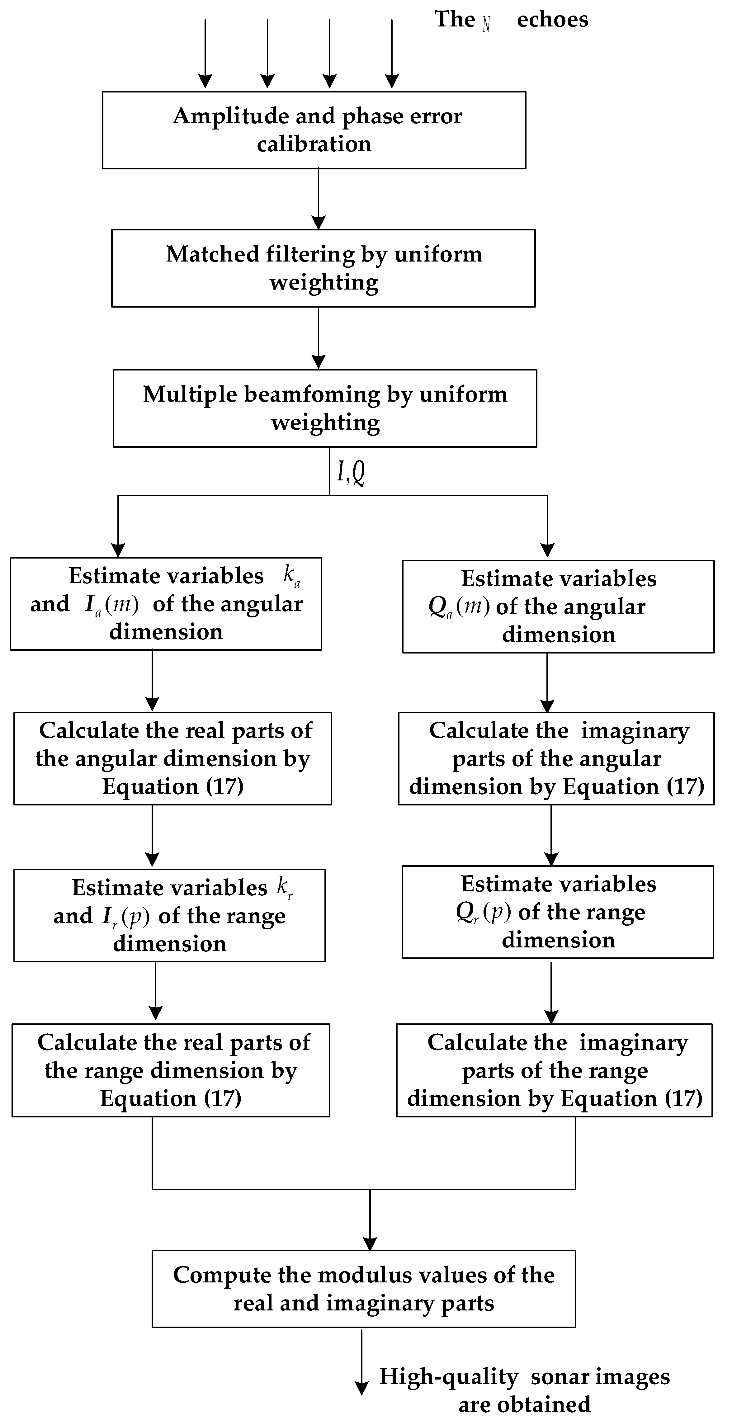
3. Improved Spatially Variant Apodization Forward-Looking Sonar Imaging Method

Sidelobe improvements can be achieved by using cosine window weighting, which decreases the main lobe resolution. DA and multiapodization can be performed to obtain a narrow main lobe; these methods can also simultaneously achieve improved sidelobes if larger numbers of weighting windows are used. Furthermore, the CDA method achieves lower sidelobes of approximately −40 dB, while also preserving the main lobe resolution. However, this method has a higher computational complexity and is less robust. Thus, the improved SVA forward-looking sonar imaging algorithm is proposed to reduce the sidelobes without degrading the main lobe resolution in angular-range dimensions.
The proposed method is a nonlinear postprocessing operation in which the raw complex-valued sonar image produced by a conventional beamformer and matched filter is weighted by a spatially variant coefficient. To enhance the robustness of the spatially variant apodization approach, the array magnitude and phase errors are calibrated to avoid beam sidelobe heightening prior to beamforming operation. The analyzed results of numerical simulations and a lake experiment demonstrate that the proposed method can greatly reduce the sidelobes to approximately −40 dB and simultaneously maintain the main lobe width. Furthermore, this method is extremely simple computationally.

3.1. SVA for Two-Dimensional Forward-Looking Sonar Imaging

To preserve the main lobe width and suppress the sidelobes, the SVA exploits the sinc function characteristics and the special properties of raised-cosine weighting functions, allowing each spatial-time sampling location in a sonar image to use its amplitude weighting function.
By combining the expression of the cosine-on-pedestal weighting window functions (7) with the beamforming output (3), the beamforming output with cosine-on-pedestal weighting can be expressed as follows:
B s ( u θ ) = 1 N n = ( N 1 ) / 2 ( N 1 ) / 2 [ 1 + w e j 2 π n N 1 + w e - j 2 π n N 1 ] * e j n d 2 π λ u θ = 1 N n = ( N 1 ) / 2 ( N 1 ) / 2 e j n d 2 π λ u θ + 1 N w n = ( N 1 ) / 2 ( N 1 ) / 2 e j 2 n π ( d u θ λ + 1 N 1 ) + 1 N w n = ( N 1 ) / 2 ( N 1 ) / 2 e j 2 n π ( d u θ λ 1 N 1 ) = sin c N d u θ λ sin c d u θ λ + w sin c N d u θ λ + N N 1 sin c d u θ λ + 1 N 1 + w sin c N d u θ λ N N 1 sin c d u θ λ 1 N 1 = sin c N d u θ λ sin c d u θ λ + w sin c N d λ u θ + λ d ( N 1 ) sin c d λ u θ + λ d ( N 1 ) + w sin c N d λ u θ λ d ( N 1 ) sin c d λ u θ λ d ( N 1 )
Using Equation (4), Equation (11) can be expressed as follows:
B s ( u θ ) = B ( u θ ) + w B ( u θ + λ d ( N 1 ) ) + w B ( u θ λ d ( N 1 ) )
According to Equation (12), the beamforming output weighted by cosine-on-pedestal functions is equivalent to the superposition of the conventional beamforming output uniform weighting and weighted shifted conventional beamforming output uniform weighting, in which the beam domain data are complex data composed of real and imaginary parts, i.e., B s ( u θ ) = I s ( u θ ) + j Q s ( u θ ) .
To effectively suppress the beam sidelobes, the SVA algorithm attempts to estimate the optimal solution   w for each special location. The real and imaginary parts of the beam domain data cannot be used to obtain the minimum value when B s ( u θ ) is simultaneously and directly calculated. However, the real and imaginary parts can be calculated separately. Then, the minimum value of the real part can be solved under the constraint of the I s ( u θ ) 2 minimum of the real part, and the minimum value of the imaginary part can be solved in the same manner. Then, the minimum value of the beam domain data can be obtained.
In the angular dimension, sample points in the beam domain are used as variables to represent the beam domain data.
B s ( m ) = B ( m ) + w ( m ) B ( m + k a ) + w ( m ) B ( m - k a )
where k a denotes the shift sampling number and is calculated with k a = λ d B ( N 1 ) d . In practical applications, k a 10 . Here, d B is the u θ spacing of adjacent beams, · denotes the downward integer operation, and B s ( m ) = I s ( m ) + j Q s ( m ) , B ( m ) = I ( m ) + j Q ( m ) .
The SVA algorithm uses the amplitude weighting method to obtain high-quality images, and its aim is to minimize the sidelobe while preserving the main lobe. For the real part of the beam domain data, the minimum I s ( m ) 2 , subject to         0 w I ( m ) 1 / 2 , is applied in the SVA algorithm to estimate the optimal solution w I ( m ) , which is expressed as follows:
min w I ( m ) I s ( m ) 2 s . t .     0 w I ( m ) 1 / 2
I ( m ) is assumed to be a real-valued component, and w I ( m ) can also be obtained by directly solving for I s ( m ) = 0 . Then, solving for w I ( m ) minimizes I s ( m ) 2 , and w I ( m ) can be determined with the unconstrained w I ( m ) as follows:
w I ( m ) = I ( m ) I ( m + 1 ) + I ( m 1 )
By inserting Equation (15) into Equation (13) and constraining w I ( m ) in (15) to 0 w I ( m ) 1 / 2 , and combining the properties of the CDA method, the output beam domain of the sonar image by the SVA can be written as follows:
I s ( m ) = I ( m ) ,                                                                                                                                 w I ( m ) < 0 0 ,                                                                                                                                               0 w I 1 / 2 I ( m ) + ( 1 / 2 ) [ I ( m + k a ) + I ( m k a ) ] ,                     w I ( m ) > 1 / 2
Equation (16) is also independently applied to the imaginary part, and w Q ( m ) and Q s ( m ) are obtained. When w I ( m ) > 1 / 2 , I s 2 ( m ) is expressed as:
I s 2 ( m ) = I 2 ( m ) 1 1 2 w I ( m ) 2 I 2 ( m )
Therefore, the beam domain SVA algorithm applies the optimal weight at the sampling point of each beam on the condition of minimizing I s ( m ) 2 and Q s ( m ) 2 independently.
B s ( m ) = B ( m ) ,                                                                                                                                 w I ( m ) < 0   0 ,                                                                                                                                               0 w I 1 / 2     B ( m ) + 1 / 2 B ( m + k a ) + B ( m - k a ) ,                     w I ( m ) > 1 / 2
Thus, the main lobe of the beam can be preserved, and the sidelobe of the beam can be suppressed. To further reduce the computational burden, the variables I a ( m ) are assumed to be:
I a ( m ) = 1 / 2 [ I ( m + k a ) + I ( m k a ) ]
The weight w I ( m ) and the SVA output I s ( m ) , normalized by I a ( m ) , are expressed as:
w I ( m ) = 0 ,                     I a ( m ) I ( m ) 0 I ( m ) / I a ( m ) / 2 ,                     I a ( m ) I ( m ) < 0   &   I ( m ) < I a ( m ) 1 / 2 ,                   else                     ( a ) I s ( m ) / I a ( m ) = I ( m ) / I a ( m ) , I a ( m ) I ( m ) 0 0 , I a ( m ) I ( m ) < 0   &   I ( m ) < I a ( m ) 1 + I ( m ) / I a ( m ) , else                           ( b )
According to Equation (20), assuming that I ( m ) is within a main lobe, I ( m ) and I a ( m ) have the same signs, I a ( m ) I ( m ) 0 and w I ( m ) = 0 , i.e., the beam main lobes are preserved. When I ( m ) is within an area of pure sidelobes, I ( m ) and I a ( m ) have opposite signs, I ( m ) < I a ( m ) , and 0 w I ( m ) 1 / 2 , i.e., the beam sidelobes are completely suppressed. Assuming that I ( m ) is in an area of a beam main lobe superimposed with beam sidelobes, I ( m ) and I a ( m ) have opposite signs and I ( m ) > I a ( m ) , w I ( m ) = 1 / 2 , i.e., the beam domain data are suppressed somewhat in an attempt to reduce the impact of the beam sidelobes.
Combined with Equations (16) and (20), the beam domain SVA algorithm output can also be expressed as follows:
I s ( m ) = I ( m ) , I a ( m ) I ( m ) 0 0 , I a ( m ) I ( m ) < 0   &   I ( m ) < I a ( m ) I ( m ) + I a ( m ) , else
Moreover, the real and imaginary parts of the SVA algorithm are equivalent to those of the CDA algorithm. The beam domain data are weighted w I ( m ) and w Q ( m ) by the point amplitude to realize the apodization process, and a high-quality acoustic image is obtained. Hence, after processing by the SVA method, the beam main lobe is preserved with a beam width equal to that of conventional beamforming θ B W = 50.7 λ / ( N d ) , and the sidelobe levels are approximately equal to zero and lower than −40 dB. In practical engineering, for forward-looking sonar imaging, high-quality acoustic images can be obtained with the sidelobe levels lower than −40 dB.
From Equation (21), the sidelobes of the beamforming results are set to exactly zero by the SVA, but the main lobes are preserved. Therefore, the sidelobes are suppressed without degrading the main lobe width in the angular dimension using the SVA method.
Since the output envelope matching filter in the range dimension is also in the form of a sinc function, lower sidelobes can be achieved, while the main lobe resolution can be preserved by using the SVA algorithm.
The effects of frequency–domain cosine window weighting and time–domain cosine window weighting for distance sidelobe reduction are essentially the same. Furthermore, using the property of the Fourier transform, the matching template of the frequency–domain window functions can be represented as follows:
H ( f ) = w ( f ) s * ( f )
where w ( f ) is the cosine base window function with respect to f , and s ( f ) is the frequency domain of the transmitted pulse signal. Thus, the matched filter output using the frequency–domain window weighting can be expressed as follows:
R ( f ) = s ( f ) H ( f ) = s ( f ) s * ( f ) w ( f )                   = s ( f ) s * ( f ) 1 + w e ( j 2 π f B ) + w e ( - j 2 π f B )                   = R ( f ) + R ( f ) w e ( j 2 π f B ) + R ( f ) w e ( - j 2 π f B )
Equation (23) is transferred to the time domain as follows:
R ( t ) = R ( t ) + R ( t + 1 / B ) + R ( t 1 / B )
According to Equation (24), the matched filter output weighted by cosine-on-pedestal functions is equivalent to the superposition of the conventional matched filter output uniform weighting and weighted shifted conventional matched filter output uniform weighting. Then, the sonar image range dimension discrete output by the SVA can be expressed as follows:
R s ( p ) = R ( p ) + w R ( p + k r ) + w R ( p - k r )
where p represents the samples in the range dimensions, k r denotes the shift sampling number, k r = 1 T s B , and T s is the sampling rate time domain of the echoes. According to the matched filter theory, the relationship between the main lobe width and bandwidth determined by the conventional method can be expressed as Δ r M L = c 2 B . Δ r M L is the main lobe width, and   c is the underwater acoustic velocity. Then, the main lobe width of the SVA method in the range dimension is equal to that of the conventional method, and the and the sidelobe levels are approximately equal to zero, lower than −40 dB.
In the SVA method, the raw complex-valued sonar image data are first obtained via uniform weighing. Subsequently, for the real parts of the angular dimension, the variables k a and I a ( m ) are calculated. Then, the real parts of the SVA algorithm are obtained via Equation (21), and the imaginary parts of the angular dimension, are processed in the same manner. Similarly, the range dimension sonar image data are performed and the reduced sidelobe levels data are obtained.
For the computational burden of conventional multibeamforming, it can be estimated that, per sample, the complex multiplication number is N B N ( N B is the number of beams), and the addition number is N B ( N 1 ) . The time consumption of complex multiplication is far greater than that of the addition of a digital signal processor or computer, and N B is far greater than N , so the computational complexity of the conventional multibeamforming method is O [ N B ] . For the angular dimension of the SVA method, compared with the conventional beamforming method, the increase in the multiplication number is 2 N B , and the increase in the addition number is approximately 2 N B . Hence, the computational complexity of the SVA method in the angular dimension is also O [ N B ] .
For the matched filtering process, for each element, the computational complexity of the FFT is between O [ N T ] and O [ N T 2 ] ( N T is the number of time samples). For the SVA method in the range dimension, compared with the conventional method, the increased multiplication number is 2 N T , and the increased addition number is approximately 2 N T . Hence, the computational complexity of the SVA method in the range dimension is also between O [ N T ] and O [ N T 2 ] .
According to the above derivation, we propose a two-step SVA algorithm in which sonar imaging is first applied to the angular dimension and then to the range dimension. This process achieves sonar imaging with angular-range sidelobe suppression, while preserving the angular-range resolution.

3.2. Amplitude and Phase Error Calibration

In practical engineering, the magnitude and phase errors of sonar arrays are always present due to their nonideal status. In this case, sidelobe heightening occurs, resulting in the deviation in the output of the envelope of the angular-range dimensions from the theoretical values. Thus, the SVA algorithm is less robust, and the array amplitude and phase inconsistencies should be calibrated prior to the use of the SVA algorithm.
The array phase difference ψ n represents the measured phase difference, which is the sum of the additional phase shift φ n caused by array channel nonuniformity and the geometric phase difference ϕ n caused by the sound path difference, i.e., ψ n = ϕ n + φ n .
In practice, the geometric phase difference ϕ n can be calculated based on the sonar array parameters. Assuming that a sound source is located at the r s , θ s near field, the additional phase shift φ n can be calibrated by minimizing an appropriate cost function as follows:
ϒ = min r s , θ s n = 1 N [ ψ ^ n 2 π λ ( r n r s ) ] 2
where r n is the distance between the sound source and the   n th receiver. Equation (26) is estimated by adopting least squares of the phase difference, and when the value of ϒ is minimal, the location of the source can be precisely estimated. Within the preset position range of the sound source, the minimum value has unique convergence, that is:
ϒ r = 0 ϒ θ = 0
Then, the additional phase shift of the   n th receiver φ n can be obtained as follows:
φ ^ n = ψ ^ n 2 π λ [ r ^ s 2 + d n 2 2 r ^ s d n sin θ ^ s ] 1 / 2 r ^ s
where θ ^ s and r ^ s are the angle and range of the sound source estimated by Equation (26), respectively. To improve the measurement accuracy of the phase difference, phase inconsistencies are usually measured and calculated at multiple angles of the sound source.
Multiple samples of the sound source direct wave signal received by each element are averaged, and the amplitude of each element is estimated as follows:
A n = 1 K i = 1 K x n ( t i )
where K denotes the number of samples. The amplitude of the reference matrix element is subtracted to obtain the amplitude inconsistency.
According to the estimated phase inconsistency φ ^ n and the amplitude inconsistency Δ A ^ n between array elements, the array amplitude and phase inconsistency calibrated matrix can be expressed as follows:
Γ ^ = diag 1 ( 1 + Δ A ^ 1 ) e - j Δ φ ^ 1 , 1 ( 1 + Δ A ^ 2 ) e - j Δ φ ^ 2 , 1 ( 1 + Δ A ^ n ) e - j Δ φ ^ n , , 1 ( 1 + Δ A ^ N ) e - j Δ φ ^ N
where Γ ^ 1 Γ ^ = I N compensates for the beamforming weighting vector and I N denotes unit matrix. The calibrated beamforming results obtained using Γ ^ are close to the theoretical sinc function values, enhancing the robustness of the SVA algorithm. The amplitude and phase errors are compensated before sonar imaging, and its time consumption has little effect on real-time imaging.
The amplitude and phase errors in the range dimension are ignored here due to the complicated underwater propagation environment, and further research will be conducted in the future. In the proposed method, the amplitude and phase inconsistency are first calibrated. Then, a two-step SVA is applied to the azimuth-range dimensions. Compared with the conventional imaging method, the proposed method also includes addition, multiplication, and comparison operations, and there is no iterative loop operation. The computational cost of the proposed method is similar to that of conventional imaging methods, which is beneficial for real-time imaging applied in engineering. Therefore, the sidelobe levels are suppressed without sacrificing the main lobe resolution by the improved SVA algorithm for forward-looking sonar imaging, which is extremely simple computationally and more robust.
A flowchart outlining the proposed algorithm is depicted in Figure 4.

4. Simulation and Experimental Results

In this section, we mainly analyze sonar single-ping imaging, where the conventional method, CDA method and proposed improved SVA method are employed, and a comparative study is conducted via simulations and a lake experiment.

4.1. Simulation Results

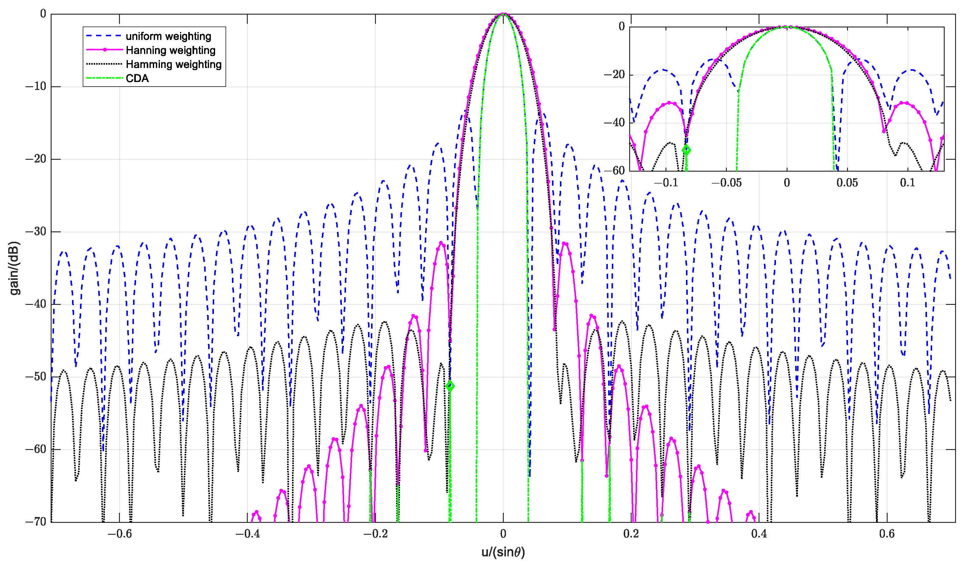
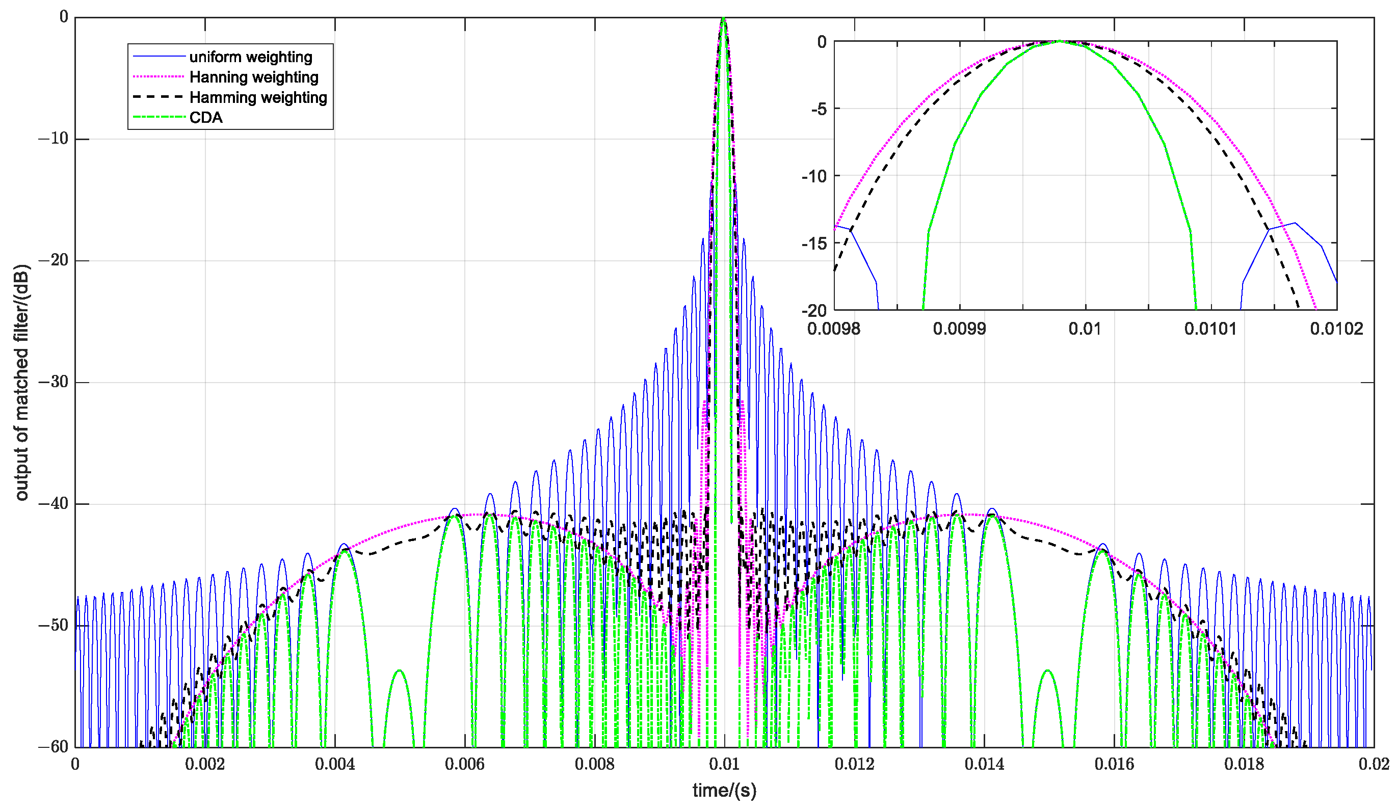
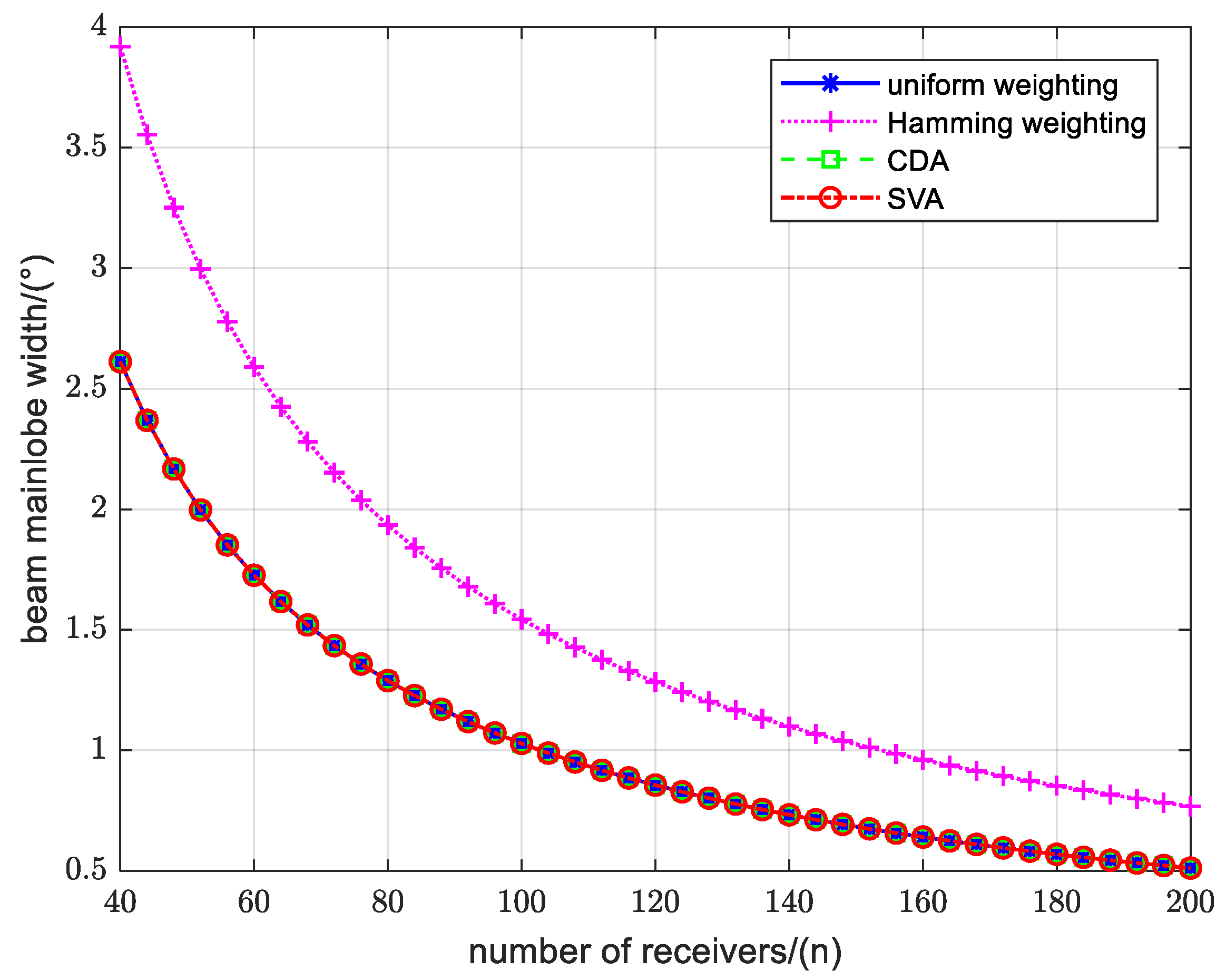
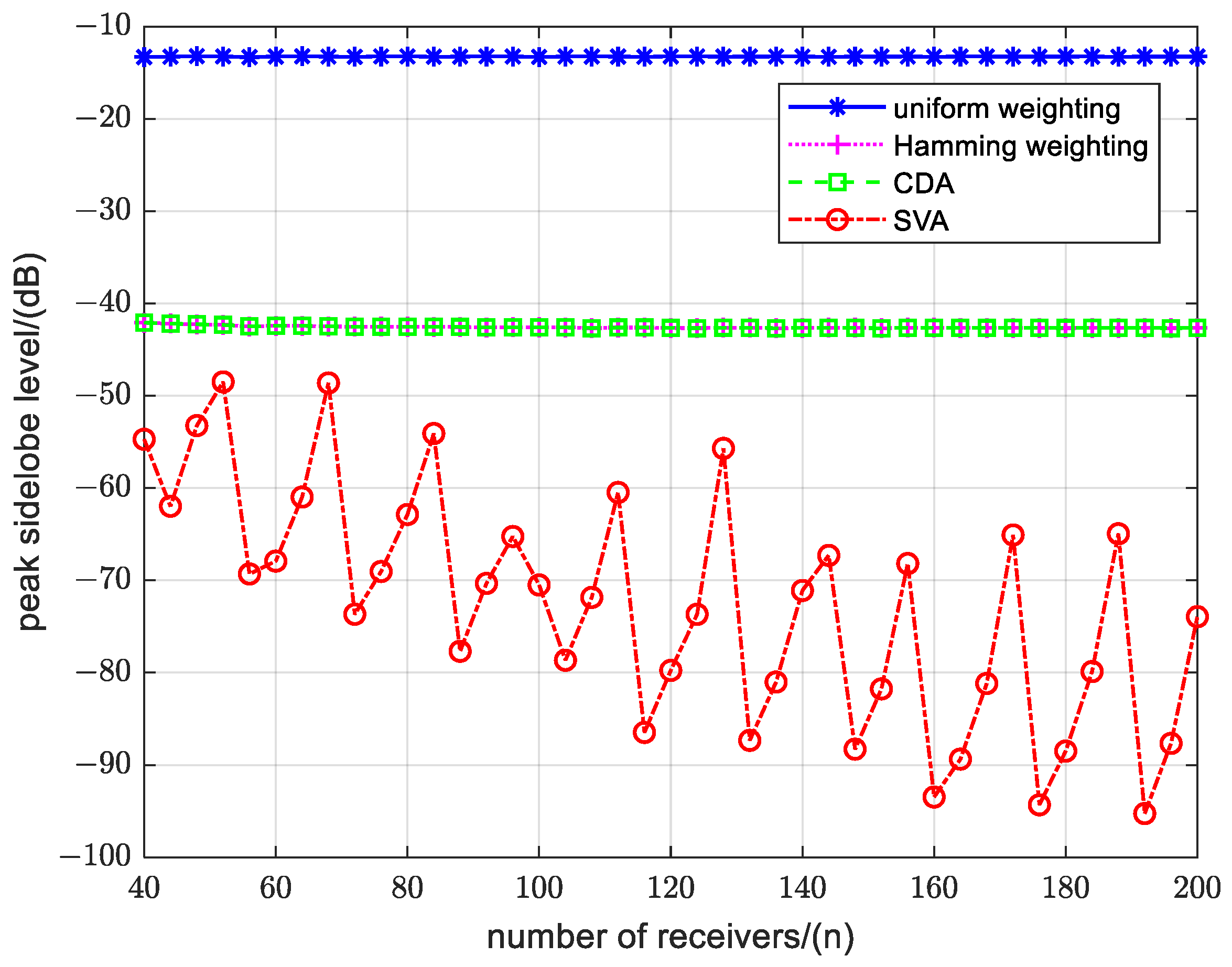
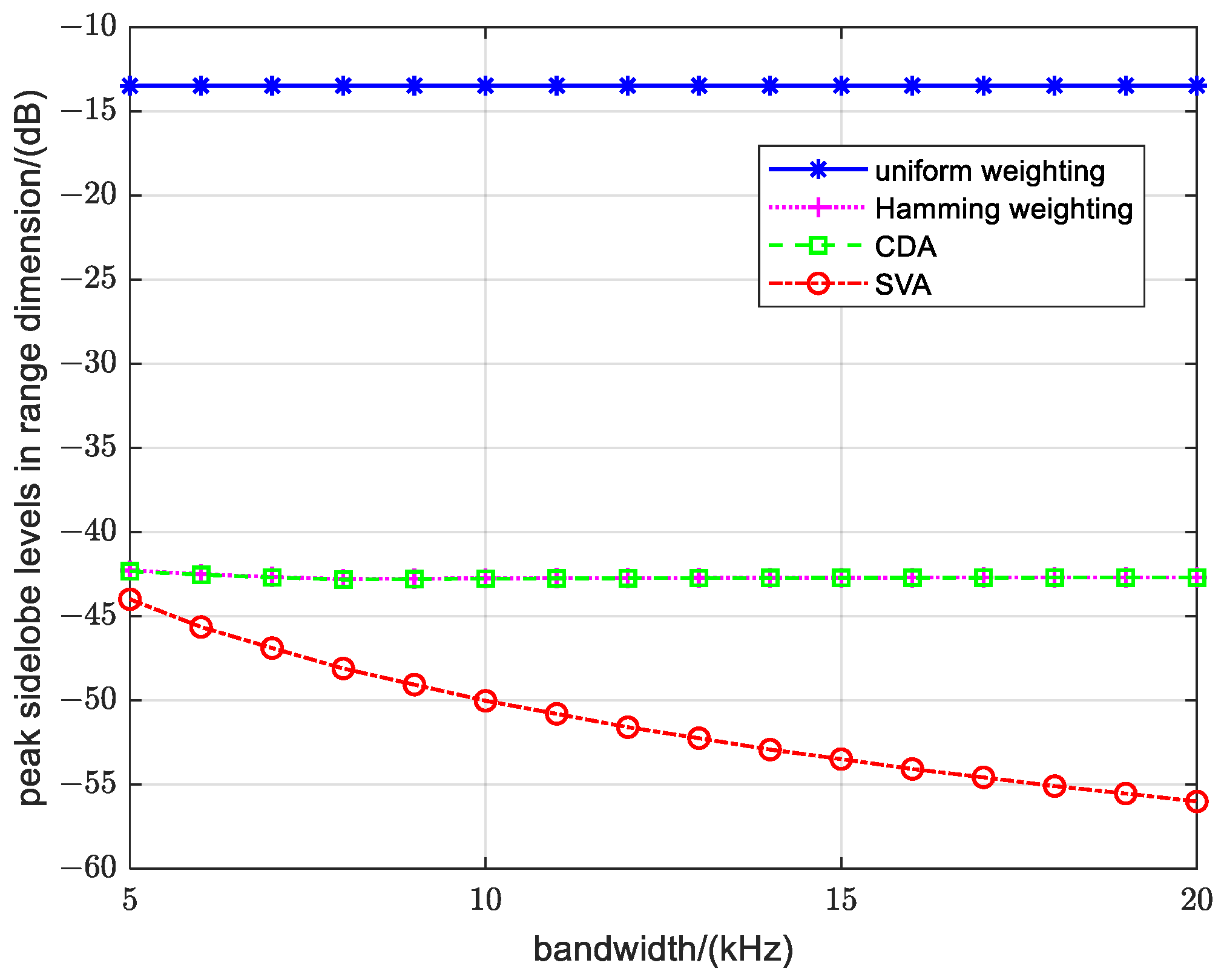
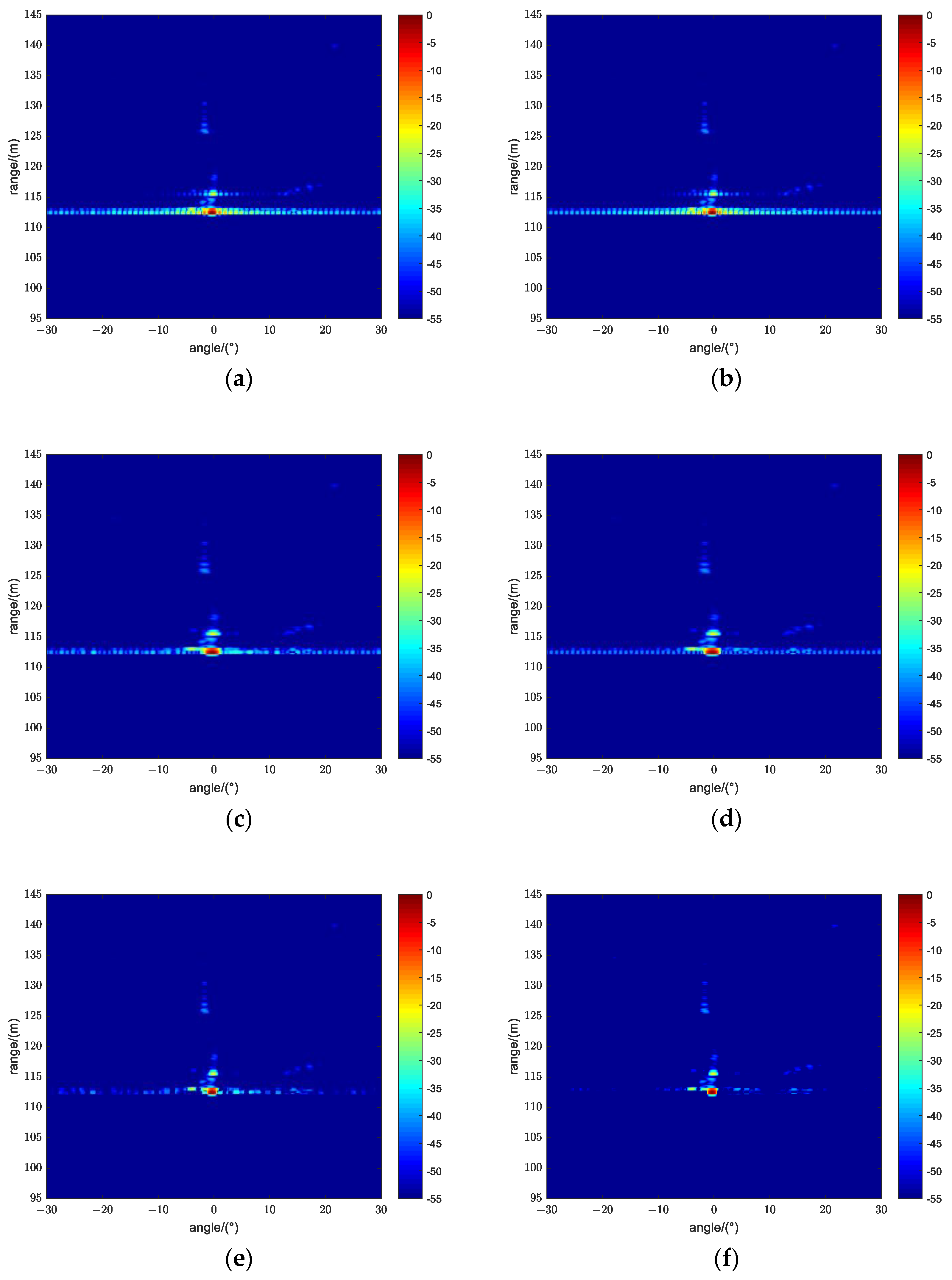
4.1.1. Analysis of the Resolutions and Sidelobes

A ULA spacing half wavelength with elements from 40 to 200 is considered and the carrier frequency of the imaging sonar is 80 kHz. The dependences of the beam main lobe widths and peak sidelobe levels on the number of receivers are investigated by uniform weighting, Hamming weighting, CDA and SVA. The corresponding results are given in Figure 5 and Figure 6, respectively.
It is clear that the beam main lobe widths of the CDA and SVA are both consistent with those of the uniform weighting method with 40 to 200 receivers. Moreover, the beam peak sidelobe levels (PSLs) of the CDA and SVA are both lower at −40 dB compared to the PSL of the uniform weighting method, which is approximately −13 dB. However, the sidelobe levels are reduced with decreasing main lobe resolution via Hamming weighting.
Since the carrier frequency of the imaging sonar is 80 kHz, the transmitted signal is a linear frequency modulation signal. Additionally, the pulse width is 40 ms, and the bandwidth changes from 5 kHz to 20 kHz. The outputs of matched filtering are obtained by using uniform weighting, Hamming window weighting, CDA processing, and SVA processing methods. The simulation results of the main lobe width and the peak sidelobe level are shown in Figure 7 and Figure 8, respectively.
Figure 7 shows that the main lobe width of the target point in the range dimension is related to the bandwidth of the transmitted signal, where the main lobe width obtained by the SVA method is consistent with that of the conventional method and is also consistent with the theoretical value, e.g., when the bandwidth is 10 kHz, the main lobe width is 0.075 m. Therefore, the relationship between the main lobe width and bandwidth for different methods is nonlinear. As shown in Figure 8, in the bandwidth range of 8 kHz to 20 kHz, the main lobe and sidelobe ratios obtained by using the conventional method are approximately 13 dB, while the main lobe and sidelobe ratios obtained by the SVA method are approximately 40 dB. Furthermore, the range dimension SVA method can also achieve lower sidelobe levels while maintaining the same main lobe width.

4.1.2. Analysis of the Array Gain

The improvement of the output signal-to-noise ratio (SNR) between the SVA method and CBF beamforming is estimated analytically by adopting the array directivity index, which is defined as the array gain in isotropic noise according to:
AG sva = 10 log 10 2 1 1 B p _ s v a 2 ( u θ ) d u θ
where B p _ s v a 2 ( u θ ) denotes the beam power of the SVA algorithm. The array gain versus the number of receivers is simulated using uniform weighting, Hamming window weighting, CDA and SVA. The carrier frequency of the imaging sonar is 80 kHz in the simulation, and the corresponding results are shown in Figure 9. The simulation results clearly demonstrate that the AG of the uniform weighting method yields a 10 log 10 ( N ) theoretical curve, while the AG of the Hamming window weighting method decreases. Nevertheless, compared with that of the uniform weighting method, the AG of the SVA method slightly increases by approximately 0.5 dB.

4.1.3. Analysis of the Quality of Sonar Images

The FLS array is composed of a transmitter and an 80-receiver ULA, and the carrier frequency of the imaging sonar is 80 kHz. The transmitted pulse is LFM with a bandwidth of 8 kHz and a pulse length of 40 ms, where the SNR is assumed to be 40 dB. The two-dimensional uniform weighting separately method, two-dimensional cosine window weighting separately method, and one-dimensional two-step SVA are processed, and sonar images are obtained. Additionally, the angular dimension slices and range dimension slices of the sonar images are obtained.
The 2-D sonar images and the target slices are shown in Figure 10. Figure 10a shows the sonar image when the angular and range dimensions are weighted by the uniform method separately. Notably, the sidelobe levels in the two dimensions around the targets are higher, causing the target images to be blurry. Figure 10b presents the image result obtained by the angular and range dimensions Hamming function weighting method, where the sidelobe levels are suppressed at the expense of strongly decreased resolution. Figure 10c shows a sonar image obtained by the proposed method, in which the sidelobe levels around the targets are reduced considerably to −40 dB with no changes the resolution in two dimensions, resulting in enhanced targets. Furthermore, Figure 10d,e show the angular slice and range slice of the sonar images at the target, where the sidelobe levels in two dimensions are −40 dB while the main lobe width remains unchanged.

4.1.4. Analysis of the Computational Burden

To analyze the computational burden of the proposed method, the computational times of the conventional uniform weighting method, cosine window weighting method and one-dimensional two-step SVA method are given in Figure 11, and the matrix size of the raw image is 256 × 1667 . A PC with an Intel (R) Core (TM) i7-10510U CPU @ 1.8 GHz was used, and the computation times were obtained by the MATLAB functions CLOCK and ETIME.
In Figure 11, the results are the average values of 50 repeated runs. For the sonar array number of 100, the computation times for both conventional window weighting methods were approximately 0.4 s. The one-dimensional SVA sequential processing method involves postprocessing of the raw image data with extremely simple computations, and the calculation amount is slightly greater than that of the conventional methods; therefore, the proposed SVA method is particularly suitable for real-time imaging.

4.1.5. Analysis of the Robustness

In this simulation, the amplitude and phase errors in the angular dimension of the system and the environmental errors are considered. Assuming that a receiving ULA of 80 elements is a spaced at half-wavelength, the array amplitude and phase errors are Gaussian distributed with variances equal to (1 dB, 5°) and (2 dB, 10°), respectively. The output beamforming is shown in Figure 12.
As shown in Figure 12, for both the window weighting methods and the SVA method, the performance decreases with beam sidelobe levels higher than −30 dB in the presence of array amplitude and phase errors. In contrast, the proposed improved SVA method combining the amplitude and phase error calibration method with the SVA method is not sensitive to the amplitude and phase errors, and the main side lobe ratio of the beam pattern is greater than 40 dB, indicating its high robustness.

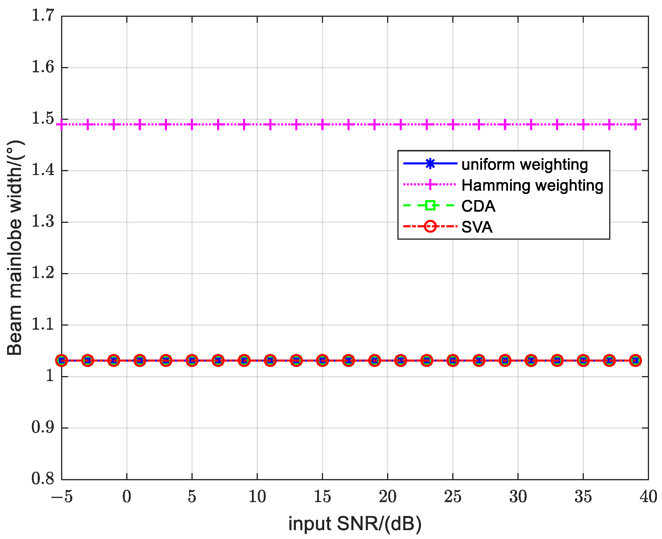
4.1.6. Analysis of the Algorithm Performance with Respect to the SNR

Considering that a receiving ULA of 100 elements is a spaced at half-wavelength, the carrier frequency of the imaging sonar is 80 kHz. The beam main lobe widths and peak sidelobe levels versus the input SNR are investigated by uniform weighting, Hamming weighting, CDA and SVA. The corresponding results are given in Figure 13 and Figure 14, respectively.
According to the results presented in Figure 13 and Figure 14, the beam main lobe widths of the proposed SVA method are consistent with those of the uniform weighting method over a wide input SNR range, while those of the Hamming weighting method are wider. When the input SNR is less than 0 dB, the peak sidelobe levels of the proposed SVA method are essentially the same as those of the uniform weighting method. With the increase in the input SNR, the peak sidelobe levels of the proposed SVA method are lower than those of the uniform weighting method. CDA shows the same performance as the proposed SVA method, but its computational burden is greater.
As shown from the above simulations and analysis, compared to the uniform weighting method, cosine window weighting method and CDA method, the proposed method can reduce the sidelobes without degrading the main lobe width for forward imaging sonar in a wide input SNR and slightly increases the array gain, leading to a satisfactory improvement in the image quality. Additionally, the proposed method has good robustness and a low computational cost.

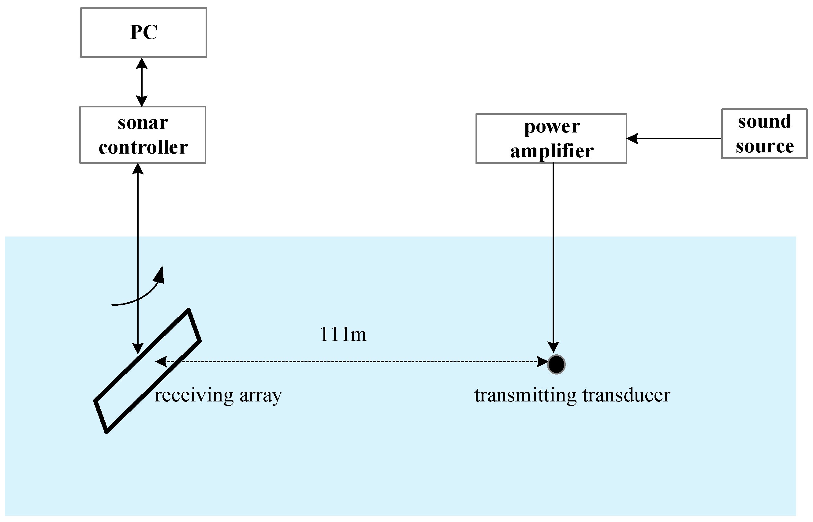
4.2. Lake Experimental Data Processing Results

A lake experiment for forward-looking sonar imaging was conducted to evaluate the proposed improved SVA method. The water depth in the experimental area was approximately 65 m. In this section, first, the array amplitude and phase errors are analyzed and calibrated. Then, improved sonar images with low sidelobes and an unchanged resolution are obtained by processing the experimental data using the improved SVA method. The sonar system, which is composed of a transmitter and an 80-receiver ULA, is suspended 5 m underwater by a connecting rod from an anchored ship. The sonar system is applied to detect underwater targets and lake-bottom mountains.

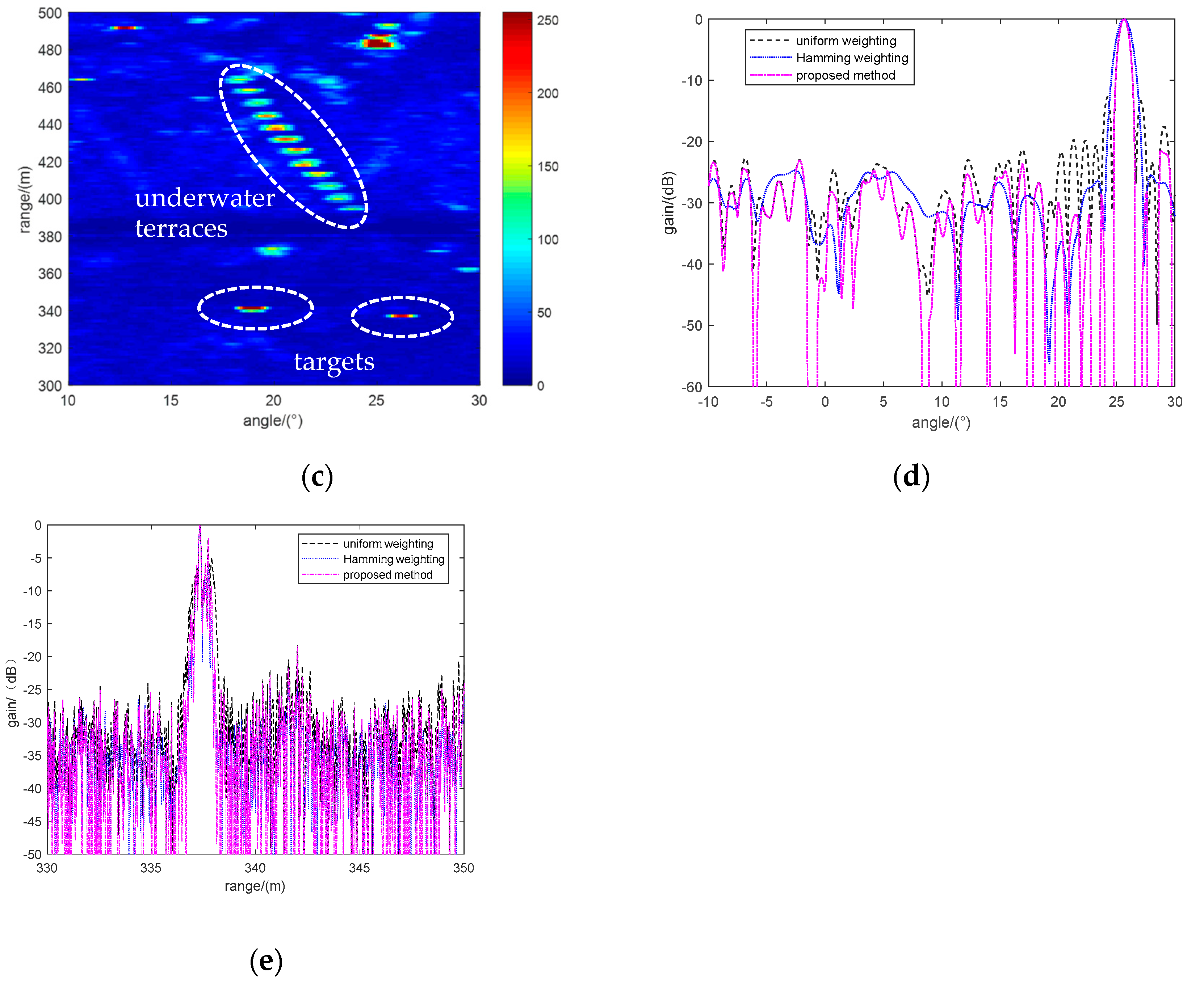
4.2.1. Analysis of Calibration and Point Scatterer Imaging Results

The underwater sound source is placed underwater at the same depth as the sonar array with a horizontal distance of approximately 111 m, and a view of the lake calibration experiment is shown in Figure 15. The sound source emission signal is a single-frequency short pulse when the direct wave is selected for analysis and processing.
Based on the position of the sound source, the least squares estimation method is used to estimate the phase errors and amplitude errors. The underwater sound source is assumed to be the ideal point scatterer target. Then, the imaging performances of the uniform weighting method [7,9], Chebyshev weighting method [9], and improved SVA method before and after amplitude and phase error calibration are compared, and the experimental results are shown in Figure 16.
Figure 16 shows the imaging results of the underwater sound source target between the uncalibrated and the calibrated arrays using three methods for lake experiments. A comparison of the sonar image obtained by the conventional uncalibrated uniform weighting method presented in Figure 16a, and the sonar image generated by the uncalibrated Chebyshev window weighting method presented in Figure 16b shows that the beam sidelobe levels are reduced when increasing the beam width, while the beam sidelobe levels obtained by the proposed method are suppressed with the beam width, approximately equal to that of the image in Figure 16a. Figure 16b,g show that the calibrated beam pattern envelope is closer to the sinc function and that the beam sidelobe levels are lower when uniform weighting is used. Moreover, the sidelobe levels are lower (−40 dB) after calibration but have greater main lobe width. For SVA filtering, the beam sidelobe levels after calibration are all below −45 dB, and the azimuth resolution remains unchanged. Hence, the proposed improved SVA method can successfully obtain images of the point scatterer target; simultaneously, it has high robustness.

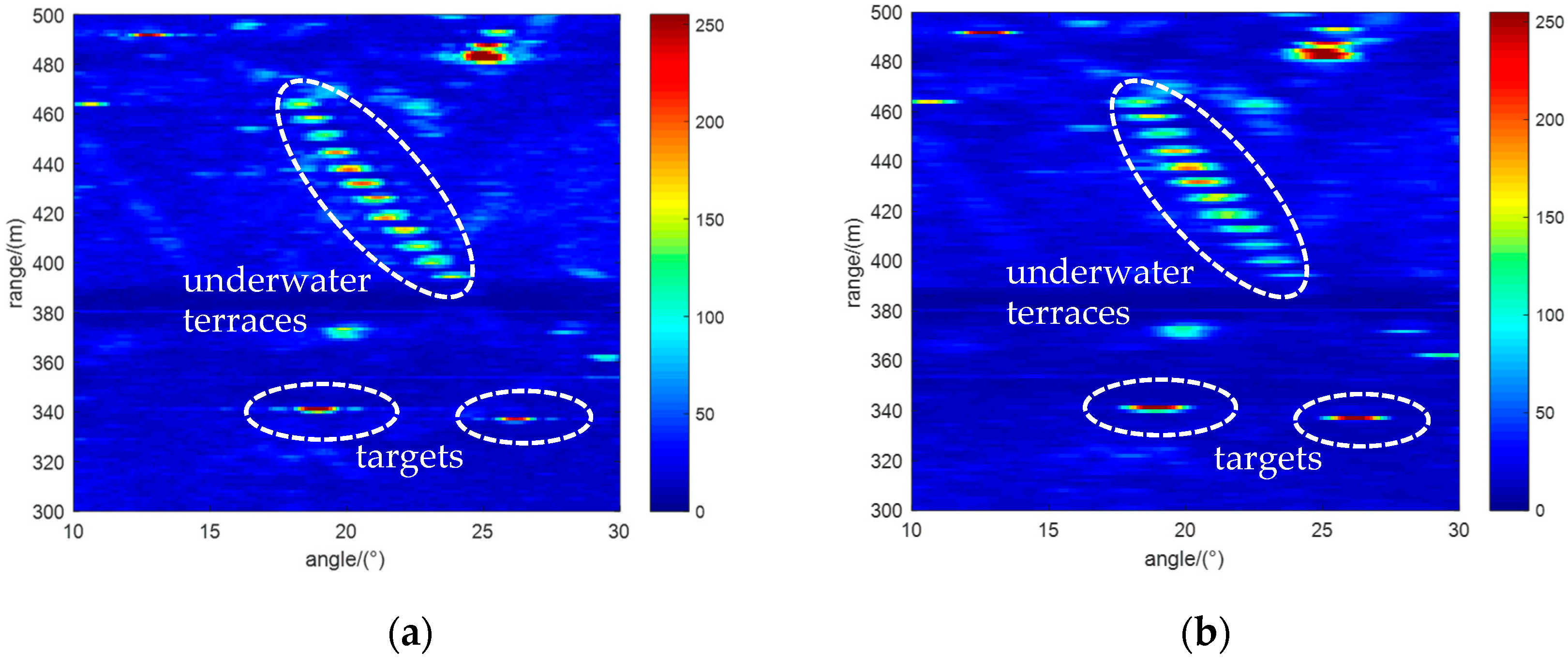
4.2.2. Analysis of Imaging Results for the Whole Target Scene

The transmitted signal of the FLS is an LFM pulse with a carrier frequency of 80 kHz, and the receiving array mainly receives the reflected echoes of targets and mountains in the water. The layout and scene of the lake experiment are shown in Figure 17. After calibrating the amplitude and phase errors of the array echo signal, the conventional imaging method [7,9], the azimuth-range Hamming window weighting imaging method [9], and the azimuth-range two-step SVA imaging method are used. The imaging results are shown in Figure 18.
Figure 18 shows the sonar images of the underwater mountains and underwater targets processed by the three methods. A comparison of the sonar image obtained by the conventional method presented in Figure 18a and the sonar image generated by the proposed method presented in Figure 18c shows that the two-dimensional resolution of the image in Figure 18c is approximately equal to that of the image in Figure 18a, and the azimuth-range dimension sidelobe levels are effectively suppressed, with sidelobe levels approximately equal to those in Figure 18b. Furthermore, Figure 18d shows the azimuthal section of the underwater target at a distance of 337 m, and it is observed that the beam main lobe width remains unchanged at approximately 0.9°. Due to the influence of underwater reverberation and noise, the beam sidelobe levels near the target point are approximately −30 dB. Figure 18e shows the range dimension of the underwater target at an azimuth of 26°. At the same time, the proposed method partly reduced the sidelobe levels near the target point. However, with the influence of the high complexity of underwater acoustic channel propagation and the frequency fluctuation characteristic of transmitting-receiving transducers, the echo LFM waveforms deviate from the theoretical waveforms, so the range dimension sidelobe suppression effect of the SVA method is not evident in practice. Further research on the impact of underwater acoustic channel propagation on the emission waveform can be carried out to improve the algorithm. The above analysis shows that two-dimensional lower sidelobe level sonar images with unchanged azimuth-range resolution, obtained by using an improved imaging method, improved sonar imaging performance, which is beneficial for the subsequent target detection and recognition.

5. Conclusions

Generally, the cosine window function weighting method is often used to reduce sidelobe levels for forward-looking sonar systems. This method has a lower computational cost and robustness, but it degrades the main lobe resolution. To solve this problem, we first derived the two-step SVA method for forward-looking sonar and improved its robustness to suppress sidelobes without degrading the main lobe resolution in angular-range dimensions. Through theoretical analyses, numerical simulations and lake experiment results, we have shown that the improved spatially variant apodization algorithm can adequately improve image quality by greatly reducing sidelobes while keeping the main lobe width unchanged. This process is extremely simple computationally. Due to the complex underwater environment, the range dimension sidelobe suppression performance of the SVA method decreases slightly in practice, Therefore, the propagation and variation characteristics of echoes in the range dimension will be studied in further research.

Author Contributions

Conceptualization, J.Y. and F.X.; methodology, L.Y. and F.X.; software, L.Y.; supervision, S.P. validation, L.Y. and S.P.; formal analysis, S.P.; investigation, J.Y.; data curation, F.X.; writing—original draft preparation, L.Y.; writing—review and editing, J.Y., F.X. and S.P.; funding acquisition, L.Y. All authors have read and agreed to the published version of the manuscript.

Funding

This work was funded by the IACAS Frontier Exploration Project under grant QYTS202107 and the National Key Research and Development Program of China under grant 2022YFC2806101.

Data Availability Statement

The data presented in this study are available upon request from the corresponding author. The data are not publicly available due to privacy or ethical restrictions.

Conflicts of Interest

The authors declare no conflicts of interest.

References

  1. Murino, V.; Trucco, A. Three-dimensional image generation and processing in underwater acoustic vision. Proc. IEEE 2000, 88, 1903–1946. [Google Scholar] [CrossRef]
  2. Wang, S.; Chi, C.; Wang, P.; Zhao, S.; Huang, H.; Liu, X.; Liu, J. Feature-enhanced beamforming for underwater 3-D acoustic imaging. IEEE J. Ocean. Eng. 2023, 48, 401–415. [Google Scholar] [CrossRef]
  3. Petillot, Y.; Ruiz, T.I.; Lane, D.M. Underwater vehicle obstacle avoidance and path planning using a multi-beam forward looking sonar. IEEE J. Ocean. Eng. 2001, 26, 240–251. [Google Scholar] [CrossRef]
  4. Zhou, T.; Si, J.; Wang, L.; Xu, C.; Yu, X. Automatic detection of underwater small targets using forward-looking sonar images. IEEE Trans. Geosci. Remote Sens. 2022, 60, 4207912. [Google Scholar] [CrossRef]
  5. Kiang, C.W.; Kiang, J.F. Imaging on underwater moving targets with multistatic synthetic aperture sonar. IEEE Trans. Geosci. Remote Sens. 2022, 60, 4211218. [Google Scholar] [CrossRef]
  6. Thomas, C.W. A CFAR detection approach for identifying gas bubble seeps with multibeam echo sounders. IEEE J. Ocean. Eng. 2021, 46, 1346–1355. [Google Scholar]
  7. Liu, X.; Fan, J.; Sun, C.; Yang, Y.; Zhuo, J. High-resolution and low-sidelobe forward-look sonar imaging using deconvolution. Appl. Acoust. 2021, 178, 107986. [Google Scholar] [CrossRef]
  8. Wang, P.; Chi, C.; Liu, J.; Huang, H. Improving performance of three-dimensional imaging sonars through deconvolution. Appl. Acoust. 2021, 175, 107812. [Google Scholar] [CrossRef]
  9. Van Trees, H.L. Optimum Array Processing: Part 4 of Detection, Estimation, and Modulation Theory; John Wiley & Sons Inc.: New York, NY, USA, 2002; pp. 17–79. [Google Scholar]
  10. Fredric, J.H. On the use of windows for harmonic analysis with the discrete Fourier transform. Proc. IEEE 1978, 66, 51–83. [Google Scholar]
  11. Yan, L.; Piao, S.C.; Xu, F. Orthogonal waveform separation in multiple-input and multiple-output imaging sonar with fractional Fourier filtering. IET Radar Sonar Navig. 2021, 15, 471–484. [Google Scholar] [CrossRef]
  12. Ma, C.; Sun, D.; Mei, J.; Teng, T. Spatiotemporal two-dimensional deconvolution beam imaging technology. Appl. Acoust. 2021, 183, 108310. [Google Scholar] [CrossRef]
  13. Stoica, P.; Wang, Z.; Li, J. Robust Capon beamforming. IEEE Signal Process. Lett. 2003, 10, 172–175. [Google Scholar] [CrossRef]
  14. Lønmo, T.I.B.; Austeng, A.; Hansen, R.E. Improving swath sonar water column imagery and bathymetry with adaptive beamforming. IEEE J. Ocean. Eng. 2020, 45, 1552–1563. [Google Scholar] [CrossRef]
  15. Buskenes, J.I.; Hansen, R.E.; Austeng, A. Low-complexity adaptive sonar imaging. IEEE J. Ocean. Eng. 2017, 42, 87–96. [Google Scholar] [CrossRef]
  16. Blomberg, A.E.A. Adaptive Beamforming for Active Sonar Imaging. Ph.D. Thesis, University of Oslo, Oslo, Norway, 2011. [Google Scholar]
  17. Liu, J.; Gershman, A.B.; Luo, Z.Q.; Wong, K.M. Adaptive beamforming with sidelobe control: A second-order cone programming approach. IEEE Signal Process. Lett. 2015, 10, 331–334. [Google Scholar]
  18. Gerstoft, P.; Xenaki, A.; Mecklenbräuker, C.F. Multiple and single snapshot compressive beamforming. J. Acoust. Soc. Amer. 2015, 138, 2003–2014. [Google Scholar] [CrossRef]
  19. David, G.; Robert, J.L.; Zhang, B.; Laine, A.F. Time domain compressive beam forming of ultrasound signals. J. Acoust. Soc. Amer. 2015, 137, 2773–2784. [Google Scholar] [CrossRef] [PubMed]
  20. Guo, Q.; Yang, S.; Zhou, T.; Wang, Z.; Cui, H.L. Underwater acoustic imaging via online bayesian compressive beamforming. IEEE Geosci. Remote Sens. Lett. 2022, 19, 4024505. [Google Scholar] [CrossRef]
  21. Guo, Q.; Xin, Z.; Zhou, T.; Yin, J.; Cui, H.L. Adaptive compressive beamforming based on bi-sparse dictionary learning. IEEE Trans. Instrum. Meas. 2022, 71, 6501011. [Google Scholar] [CrossRef]
  22. Yang, T.C. Deconvolved conventional beamforming for a horizontal line array. IEEE J. Ocean. Eng. 2018, 43, 160–172. [Google Scholar] [CrossRef]
  23. Yang, T.C. Deconvolution of decomposed conventional beamforming. J. Acoust. Soc. Amer. 2020, 148, 195–201. [Google Scholar] [CrossRef] [PubMed]
  24. Guo, W.; Piao, S.; Yang, T.C.; Guo, J.; Iqbal, K. High-resolution power spectral estimation method using deconvolution. IEEE J. Ocean. Eng. 2020, 45, 489–499. [Google Scholar] [CrossRef]
  25. Mei, J.; Pei, Y.; Zakharov, Y.; Sun, D.; Ma, C. Improved underwater acoustic imaging with non-uniform spatial resampling RL deconvolution. IET Radar Sonar Navig. 2020, 14, 1697–1707. [Google Scholar] [CrossRef]
  26. Sun, D.; Ma, C.; Mei, J.; Shi, W. Improving the resolution of underwater acoustic image measurement by deconvolution. Appl. Acoust. 2020, 165, 107292. [Google Scholar] [CrossRef]
  27. Liu, X.; Yang, Y.; Sun, C.; Zhuo, J.; Wang, Y.; Zhai, Q. High-angular- and range-resolution imaging using MIMO sonar with two-dimensional deconvolution. IET Radar Sonar Navig. 2023, 17, 991–1001. [Google Scholar] [CrossRef]
  28. Stankwitz, H.C.; Dallaire, R.J.; Fienup, J.R. Spatially variant apodization for sidelobe control in SAR imagery. In Proceedings of the IEEE National Radar Conference, Atlanta, GA, USA, 29–31 March 1994. [Google Scholar]
  29. Stankwitz, H.C.; Dallaire, R.J.; Fienup, J.R. Nonlinear apodization for sidelobe control in SAR imagery. IEEE Trans. Aero. Electron. Syst. 1995, 31, 267–279. [Google Scholar] [CrossRef]
  30. Zhu, R.Q.; Zhou, J.X.; Fu, Q. Spatially variant apodization for sidelobe suppression in near range radar imagery. IET Radar Sonar Navig. 2022, 16, 986–999. [Google Scholar] [CrossRef]
  31. Ding, Z.; Zhu, K.; Wang, Y.; Li, L.; Liu, M.; Zeng, T. Spatially variant sidelobe suppression for linear array MIMO SAR 3-D imaging. IEEE Trans. Geosci. Rem. Sens. 2022, 60, 5220915. [Google Scholar] [CrossRef]
Figure 1. Comparison of the beam patterns with different weighing methods.
Remotesensing 16 02100 g001
Figure 2. Comparison of the beam patterns with different weighing methods.
Remotesensing 16 02100 g002
Figure 3. Output of the matched filter with different weighing methods.
Remotesensing 16 02100 g003
Figure 4. Flowchart outlining the proposed algorithm, where the variables I r ( p ) of the range dimension are assumed to be I r ( p ) = 1 / 2 I r u ( p + k r ) + I r u ( p k r ) , and I r u ( p ) represents the real part of the uniform weighting matched filter output.
Remotesensing 16 02100 g004
Figure 5. Beam width versus the number of receivers.
Remotesensing 16 02100 g005
Figure 6. Peak sidelobe level versus the number of receivers.
Remotesensing 16 02100 g006
Figure 7. Range dimension of the main lobe width versus bandwidth.
Remotesensing 16 02100 g007
Figure 8. Range dimension peak sidelobe level versus bandwidth.
Remotesensing 16 02100 g008
Figure 9. Comparison of the array gain versus the number of receivers.
Remotesensing 16 02100 g009
Figure 10. Comparison of the 2D acoustic images obtained using different processing methods: (a) simulation image obtained by the uniform weighting method; (b) simulation image obtained by the Hamming window weighting method; (c) simulation image obtained by the proposed method; (d) results in the angular dimension corresponding to a target at 104 m; (e) results in the range dimension corresponding to a target at 12°.
Remotesensing 16 02100 g010
Figure 11. Comparison of the computing time for forming a raw image.
Remotesensing 16 02100 g011
Figure 12. Comparison of the beam patterns under different amplitude and phase errors: (a) simulation results under amplitude and phase errors (1 dB, 5°); (b) simulation results under amplitude and phase errors (2 dB, 10°).
Remotesensing 16 02100 g012
Figure 13. Beam main lobe width versus input SNR.
Remotesensing 16 02100 g013
Figure 14. Peak beam sidelobe levels versus the input SNR.
Remotesensing 16 02100 g014
Figure 15. View of the lake calibration experiment.
Remotesensing 16 02100 g015
Figure 16. Comparison of the imaging performance between the uncalibrated and the calibrated arrays using three methods:(a) FLS image obtained by the uncalibrated uniform weighting method; (b) FLS image obtained by the calibrated uniform weighting method; (c) FLS image obtained by the uncalibrated Chebyshev window weighting method; (d) FLS image obtained by the calibrated Chebyshev window weighting method; (e) FLS image obtained by the uncalibrated SVA method; (f) FLS image obtained by the calibrated SVA method; (g) the beam response near underwater sound source corresponding to a target at 111.7 m.
Remotesensing 16 02100 g016aRemotesensing 16 02100 g016b
Figure 17. Lake experiment diagram.
Remotesensing 16 02100 g017
Figure 18. Two-dimensional images of sonar with different processing methods for sidelobe suppression: (a) FLS image obtained by the uniform weighting method; (b) FLS image obtained by the Hamming window weighting method; (c) FLS image obtained by the proposed method; (d) results in the angular dimension corresponding to a target at 337 m; (e) results in the range dimension corresponding to a target at 26°.
Remotesensing 16 02100 g018aRemotesensing 16 02100 g018b
Disclaimer/Publisher’s Note: The statements, opinions and data contained in all publications are solely those of the individual author(s) and contributor(s) and not of MDPI and/or the editor(s). MDPI and/or the editor(s) disclaim responsibility for any injury to people or property resulting from any ideas, methods, instructions or products referred to in the content.

