Communication

Lightweight Deep Neural Network with Data Redundancy Removal and Regression for DOA Estimation in Sensor Array

1
The School of Software, Northwestern Polytechnical University, Xi’an 710072, China
2
Nanjing Electronic Equipment Institute, Nanjing 210007, China
*
Author to whom correspondence should be addressed.
Remote Sens. 2024, 16(8), 1423; https://doi.org/10.3390/rs16081423
Submission received: 21 March 2024 / Revised: 14 April 2024 / Accepted: 15 April 2024 / Published: 17 April 2024
(This article belongs to the Special Issue Advanced Array Signal Processing for Target Imaging and Detection)

Abstract

:
In this paper, a lightweight deep neural network (DNN) for direction of arrival (DOA) estimation is proposed, of which the input vector is designed to remove data redundancy as well as remaining DOA information. By exploring the Vandermonde property of the steering vector of a uniform linear array (ULA), the size of the newly designed input vector is greatly reduced. Furthermore, the DOA estimation is designed as a regression problem instead of a classification problem; that is, the lightweight DNN designs the output vector as the estimated DOAs of sources, of which the size is much shorter than that of the spatial spectrum used as the output vector in the conventional DNN. The reductions in the sizes of input and output vectors lead to a reduction in the sizes of hidden layers, achieving lightweightness of the neural network. The analysis illustrates that when the number of sensors is 22, the number of parameters in the lightweight DNN is three orders of magnitude less than that in the conventional DNN. The simulation results demonstrate the lightweight DNN can provide high DOA estimation accuracy with the shortest testing time. It performs better than the conventional DNN. Furthermore, it is superior to traditional solutions such as the multiple signal classification (MUSIC) method and conventional beamforming (CBF) method in harsh conditions like low signal-to-noise ratios (SNRs), closely spaced sources, and few snapshots.

Graphical Abstract

1. Introduction

Direction of arrival (DOA) estimation is a widely studied topic in the signal processing area, which performs a key role in wireless communications, astronomical observation, and radar applications [1,2,3,4,5]. The conventional beamforming (CBF) method is a classical solution for DOA estimation. However, it suffers from Rayleigh limit. Subsequently, many traditional methods were proposed to meet the accuracy requirement and high resolution of DOA estimation, such as the minimum variance distortionless response (MVDR) beamformer (also referred to as the Capon beamformer) [6], multiple signal classification method (MUSIC) algorithm [7], estimation of signal parameters using rotational invariance techniques (ESPRIT) algorithm [8] and their variants [9,10,11,12,13]. However, the above-mentioned traditional methods require operations such as singular value decomposition and/or the inversion on the array covariance matrix of the received signal and/or spatial spectrum searching. As a result, their computational complexity is high, which makes it difficult for them to meet real-time requirements. Moreover, most of them have large estimation errors under harsh scenarios such as when the DOAs of source signals have small angular intervals or the signal-noise ratio (SNR) is low. To overcome the drawbacks of the traditional solutions, many studies use machine learning methods to solve the problem of DOA estimation, these methods first establish a training dataset with DOA labels, and then utilize existing machine learning techniques such as radial basis function (RBF) [14] and support vector regression (SVR) [15] to apply the derived mapping to the test data for DOA estimation. These methods require significant effort to learn the mapping during the training stage. However, once the mapping is learned and fixed after the training stage, they directly apply the mapping to process the testing data without labels to obtain DOA estimates. It is noted that the mapping only involves calculations of additions and multiplications, which avoids matrix inverse, decomposition, and spectrum searching. Thus, in the testing stage, they acquire higher computational efficiency compared to traditional methods [16], but they heavily rely on the generalization characteristics of machine learning technology. That is, only when the training data and test data have almost the same distribution, satisfactory test results can be obtained.
In recent years, DOA estimation based on deep learning methods has gained great attention due to its high accuracy and high computational efficiency during the testing phase. In 2015, a single-layer neural network model based on classification was designed to implement DOA estimation [17]. Since then, more and more improved neural networks aiming at solving DOA estimation have been proposed. In 2018, a deep neural network (DNN) was proposed, which contains a multitask auto-encoder and a set of parallel multi-layer classifiers, with the covariance vector of the array output as an input to the DNN, the auto-encoder decomposes the input vectors into sub-regions of space, then the classifiers output the spatial spectrum for DOA estimation [18]. In 2019, a deep convolutional neural network (CNN) was developed for DOA estimation by mapping the initial sparse spatial spectrum obtained from the covariance matrix to the true sparse spatial spectrum [19]. In 2020, a DeepMUSIC method was proposed for DOA estimation, by using multiple CNNs each of which is dedicated to learning the MUltiple SIgnal Classification (MUSIC) spectra of an angular sub-region [20]. In 2021, a CNN with 2D filters was developed for DOA prediction in the low SNR [21], by mapping the 2-D covariance matrix to the spatial spectrum labeled according to the true DOAs of source signals. In 2023, a DNN framework for DOA estimation in a uniform circular array was proposed, using transfer learning and multi-task techniques [22]. The existing results show that deep learning frameworks provide better performance than traditional methods in harsh conditions such as low SNRs and small angle intervals between the DOAs of two source signals.
It is noted that all of the above-mentioned DNN-based DOA estimation methods choose to use the whole array covariance matrix of the received signal or its upper triangular elements or their transformation as the input of the network, which contains lots of redundant information when the array is uniformly linear. In addition, most of them try to match DOA estimation with the classification problem and thus use the spatial spectrum (labeled by the true DOAs of source signals or given by the existing traditional MUSIC method) as their output vector. Therefore, in the existing DNN-based DOA estimation approaches, the data redundancy in the input vector and the large size of the output vector lead to large sizes of hidden layers and make the DNN models complex overall, resulting in low computational efficiency.
There are a few works [23,24,25] that use neural networks with regression for DOA estimation. In [23], the neural network and a particle swarm optimization (PSO) were combined for DOA estimation, which might be trapped into a minimum solution. In [24], a DNN with regression was developed to estimate the DOA of a single source signal, without considering the situation of multiple source signals. In [25], a DNN with regression was designed for DOA estimation of multiple source signals. However, it does not consider the data redundancy in a uniform linear array (ULA).
In this paper, we consider a ULA, which is the most generally adopted array geometry for DOA estimation due to its regular structure and well-developed techniques according to the Nyquist sampling theorem [26]. By exploring the property of the ULA, a lightweight DNN is proposed by designing an input vector with data redundancy removal and using the regression fashion for DOA estimation. The lightweight DNN significantly reduces the sizes of the input vector, hidden layers, and output vector, which leads to a reduction in the number of trainable parameters of the neural network and computational load. Meanwhile, the proposed lightweight DNN can preserve DOA estimation accuracy and performs better than the method in [25]. It is noted that by considering that the array signal is different from the image signal and DOA information is hidden in each element of the input vector obtained from the covariance matrix of the array signal, we utilize a fully connected deep neuron network to obtain the mapping from the input vector to the DOAs of source signals.
Throughout this paper, *, T, H, and E represent the conjugate, transpose, conjugate transpose, and expectation operations, respectively.

2. Background

Assume that K-independent far-field source signals { s k ( t ) } k = 1 K with a wavelength λ and DOAs of { θ k } k = 1 K impinge on an M-element uniform linear array (ULA) with an inter-element spacing d. Moreover, it is assumed that the source signals and the array sensors are on the same plane. The received data of the array can be expressed as
r ( t ) = A s ( t ) + n ( t ) ,
where n(t) is an additive and zero-mean white Gaussian noise vector, A = [ a ( θ 1 ) , , a ( θ K ) ] , s ( t ) = [ s 1 ( t ) , , s K ( t ) ] T ; In particular, a ( θ k ) is an M-dimensional steering vector, which is defined as
a ( θ k ) = [ 1 , e j 2 π d s i n θ k λ , , e j 2 π d s i n θ k λ ( M 1 ) ] T .
The array covariance matrix R can be expressed as
R = E [ r ( t ) r H ( t ) ] = A R s A H + σ n 2 I M ,
where R s = E [ s ( t ) s H ( t ) ] , σ n 2 is the noise power, and I M is an identity matrix with a size of M × M . In practice, due to the finite snapshots, the covariance matrix R can be estimated as
R ^ = 1 N t = 1 N r ( t ) r H ( t ) ,
where N is the number of snapshots, and ^ means the approximation of the quantity above which it appears.
Equation (4) illustrates that R ^ is a conjugate symmetric matrix. Utilizing this feature, many real-valued deep learning methods use the upper triangular elements as their input vectors [18,20]. Define the vector composed of the off-diagonal upper triangular elements of R ^ by z , that is
z = [ R ^ ( 1 , 2 ) , , R ^ ( 1 , M ) , R ^ ( 2 , 3 ) , , R ^ ( 2 , M ) , , R ^ ( M 1 , M ) ] T .
It is noted that for a real-valued DNN network, the input vector needs to be real-valued. Therefore, by concatenating the real and imaginary parts of z , we obtain z ˜ below.
z ˜ = [ R e a l ( z T ) , I m a g ( z T ) ] T / z 2 ,
where 2 defines L 2 norm. R e a l { } and I m a g { } represent the real and imaginary parts of a complex value, respectively.
In [18], a fully connected DNN method with classification was developed for DOA estimation, and it utilizes the vector z ˜ as its input, named as the conventional DNN in this paper. Note that the input vector z ˜ contains data redundancy and costs the computational load without performance improvement. Moreover, since the conventional DNN is based on classification fashion, its output is equal to θ m a x θ m i n η , where [ θ m i n , θ m a x ) is the angle-searching range of the sources, and η is the grid; with x is equal to the smallest integer not smaller than x. Therefore, the size of its output vector is much larger than the number of DOAs of sources, which further increases the computational load.
In the following, we analyze the data redundancy in the ULA and design a new input vector that removes data redundancy and retains DOA information. In a sequence, the lightweight DNN is proposed by using the newly designed input vector and employing the regression fashion for DOA estimation.

3. Data Redundancy Removal

3.1. Development of Data Redundancy Removal

In this section, we first prove that the conventional input vector z ˜ in Equation (6) contains data redundancy. Afterwards, we propose a new input vector that removes data redundancy and retains DOA information.
According to Equations (2) and (3), the array covariance matrix R can be expanded as
R = k = 1 K a ( θ k ) a H ( θ k ) σ s k 2 + σ n 2 I M ,
where σ s k 2 is the power of the k th source signal.
Define the matrix B k = a ( θ k ) a H ( θ k ) and its element at m-th row and l-th column as B k ( m , l ) . According to Equation (2), we obtain that
B k ( m , l ) = e φ k ( m l ) σ s k 2 ,
where φ k = j 2 π d sin θ k λ . Therefore, by substituting Equation (8) into Equation (7), we have
R ( m , l ) = k = 1 K B k ( m , l ) + s g n ( m , l ) σ n 2 = k = 1 K e φ k ( m l ) σ s k 2 + s g n ( m , l ) σ n 2 .
where s g n ( m , l ) = 1 i f m = l 0 i f m l . As a result, from Equation (9), we observe Lemma 1 below.
Lemma 1.
When the array is ULA, all the elements along the sub-diagonal, super-diagonal and diagonal lines of the covariance matrix R are equal.
Lemma 1 can be illustrated in Equation (10) below.
R = ρ β v ϵ β ρ β v β v ρ β ϵ v β ρ
where ρ , β , v , and ϵ are elements of the covariance matrix R .
As shown in Equation (5), the conventional input vector uses all the upper triangular elements of the covariance matrix R , which contains duplicate information and leads to data redundancy according to Lemma 1 .
On the other hand, from Equation (9), it is observed that the elements along the diagonal lines are affected by noise power and source signal power. However, they do not contain information about DOAs of sources. Thus, they shall not be involved in the input vector of the DNN model. In addition, by observing Equation (9), we define
z 1 = [ R ^ ( 1 , 2 ) , R ^ ( 1 , 3 ) , R ^ ( 1 , 4 ) , , R ^ ( 1 , M ) ] T .
By considering the above-mentioned observation, Lemma 1 , and the conjugate symmetric feature of the covariance matrix R , we obtain that indeed for a real-valued DNN model and the expected covariance matrix R , z 1 contains all the useful elements relevant to the DOAs of sources and discards duplicate data in the vector z in Equation (5), leading to the removal of data redundancy.
It is worth noticing that in practice, due to the limit of the number of snapshots, the elements along any off-diagonal line of the estimated covariance matrix R ^ are not exactly equal. On the other hand, as shown in Equation (9), the elements along each super-diagonal line contain the same information about DOAs. Thus, we propose to take the average of all the elements along each super-diagonal line of the estimated covariance matrix R ^ to obtain a new vector without data redundancy, denoted as z s u m . Define the i-th element of z s u m as z s u m ( i ) , we have
z s u m ( i ) = 1 M i m = 1 M i R ^ ( m , m + i ) , i = 1 , 2 , , M 1 .
Therefore, according to Equations (11) and (12), we can construct two vectors (that is, z ˜ 1 and z ˜ s u m ) as shown in Equations (13) and (14).
z ˜ 1 = [ R e a l ( z 1 T ) , I m a g ( z 1 T ) ] T / z 1 2 ,
z ˜ s u m = [ R e a l ( z s u m T ) , I m a g ( z s u m T ) ] T / z s u m 2 .
It is noted that both z ˜ 1 and z ˜ s u m remove data redundancy and can be used as the input vector of the DNN network theoretically. However, due to the limit of the number of snapshots in practice, the lightweight deep neural network (DNN) proposed in the following does not converge when the vector z ˜ 1 is used as the input vector of the DNN. Therefore, we choose the vector z ˜ s u m as the input of the proposed DNN in the following, which ensures convergence. On the other hand, it is noted that the conventional input vector z ˜ using upper triangular elements as shown in Equation (5) has a dimension of M ( M 1 ) . In contrast, the new input vector z ˜ s u m has a dimension of 2 ( M 1 ) . Therefore, the new input vector reduces the dimension to M / 2 times that of the conventional input vector. This implies that the nodes in the following hidden layers can be correspondingly reduced, which contributes to forming a lightweight DNN.
As a sequence, the data redundancy removal developed for the ULA above can be applied to the matrix R ^ to obtain the input vector without data redundancy (i.e., z ˜ s u m ).

3.2. Analysis of Data Redundancy Removal

According to Equations (3) and (4), R ^ is the maximum-likelihood estimate of the expected R , and thus the estimation error Δ R always exists [27]; that is,
Δ R = R ^ R .
In addition, the proposed lightweight DNN is based on the z ˜ s u m in Equation (14). In contrast, the method in [25] uses the vector composed of the off-diagonal upper triangular elements; that is, z ˜ in Equation (6). Both z ˜ s u m and z ˜ are based on the estimated covariance matrix R ^ . Consequently, these elements are also subject to estimation inaccuracies, which subsequently precipitate errors in DOA estimation. It is expected that a larger estimation error of z ˜ s u m or z ˜ leads to a higher DOA estimation error. We define the estimation error of z ˜ s u m by Δ z ˜ s u m , which is given as
Δ z ˜ s u m = z ˜ s u m z ˜ s u m e x p ,
where the elements of z ˜ s u m e x p are obtained by replacing the estimated covariance matrix R ^ with the expected one R in Equation (12).
Similarly, we define the estimation error of z ˜ by Δ z ˜ , which is written as
Δ z ˜ = z ˜ z ˜ e x p ,
where the elements of z ˜ e x p are obtained by replacing the estimated covariance matrix R ^ with the expected one R in Equation (5). Define the 2-norm of the vectors Δ z ˜ s u m and Δ z ˜ as Δ z ˜ s u m 2 and Δ z ˜ 2 , respectively.
In the following, a comparative analysis of the numerical outcomes for Δ z ˜ s u m 2 and Δ z ˜ 2 is presented. Assuming that the ULA consists of 22 elements with an inter-element spacing equal to λ 2 . Supposing that there are two source signals with the same SNR impinge onto the array with DOAs of θ 1 = 40.55 and θ 2 = 36.3 , respectively. The number of snapshots equals 400. The number of trials is 200.
When SNR = −10 dB, we obtain Δ z ˜ s u m 2 = 0.19 , and Δ z ˜ 2 = 0.37 . When SNR = 5 dB, we obtain Δ z ˜ s u m 2 = 0.06 , and Δ z ˜ 2 = 0.09 . Overall, Δ z ˜ s u m 2 < Δ z ˜ 2 . This fact leads to better performance of the proposed lightweight DNN with its input as z ˜ s u m , as comparisons of the method in [25] with its input as z ˜ . This fact matches with numerical results in Section 5.
Furthermore, from the analysis above, we obtain that Δ z ˜ s u m 2 decreases as the SNR increases, which implies that the performance of the lightweight DNN with z ˜ s u m gets better as the SNR increases.

4. Lightweight DNN for DOA Estimation

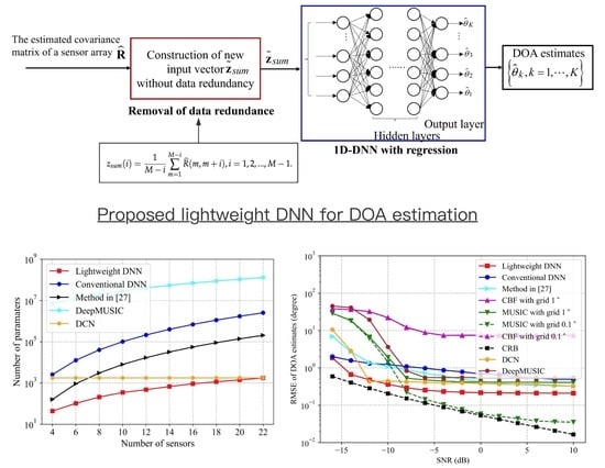
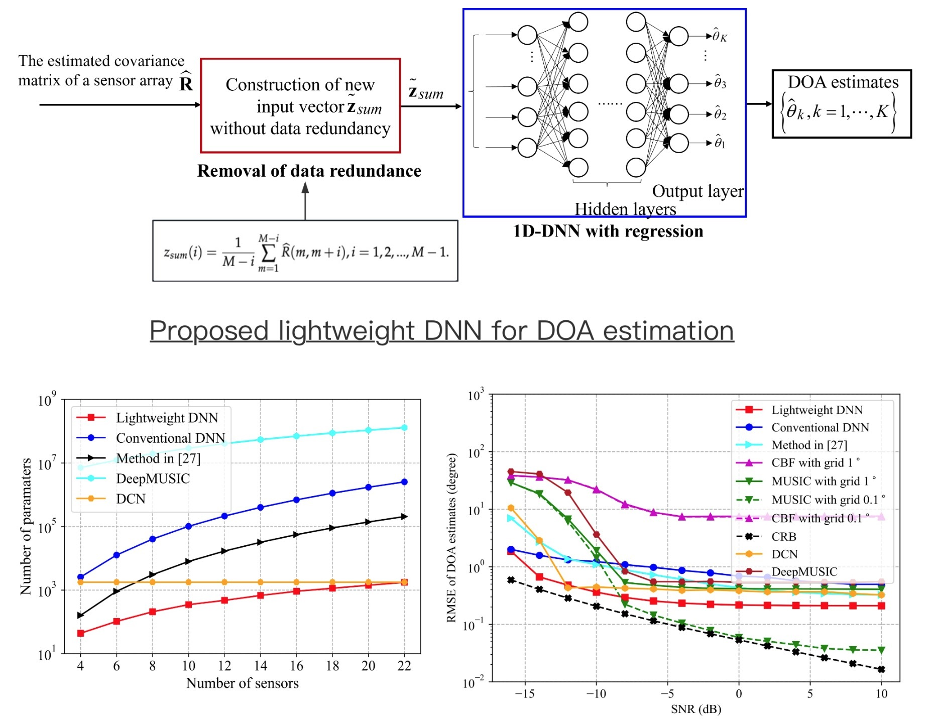
In this section, we propose a lightweight DNN for DOA estimation, which is illustrated in Figure 1. As shown in Figure 1, the proposed lightweight DNN model utilizes the newly developed input vector z ˜ s u m as its input vector. Furthermore, different from the conventional DNN model with classification [18,19,20,21], the new DNN model is a regression model and has an output vector with a dimension equal to the number of sources, which approaches to the vector of true DOAs of sources in a regression fashion. It is noted that by considering the DOAs of sources are continuous values, the DNN model with regression can match the task of DOA estimation naturally. It is noted that in practice, prior to DOA estimation, the estimation of the number of sources can be accomplished by the classical methods such as the Minimum Description Length (MDL) and the Akaike Information Criterion (AIC) methods [28]. In addition, by considering that the array signal is different from the image signal and DOA information is hidden in each element of the input vector which is obtained from the covariance matrix of the array signal, we select a fully connected deep neuron network to extract the mapping from the input vector to the DOAs of source signals.
As shown in Figure 1, the proposed lightweight DNN is a fully connected network with regression and contains an input layer, several hidden layers with activation functions, and an output layer. Furthermore, each node of each layer in the network is connected to each node of the adjacent forward layer. The input data flows into the input layer, passes through the hidden layers, and turns into the output of the network, which gives DOA estimates. The detailed structure of the proposed lightweight DNN model and its construction of the training data set are given as follows. It is noted that both the proposed lightweight DNN method and the method in [25] use regression for DOA estimation. The difference between the proposed lightweight DNN method and the one in [25] is that the proposed lightweight DNN method removes the data redundancy and significantly reduces the trainable parameters, by analyzing the property of the covariance matrix of a ULA and the parameters of the network.

4.1. Detailed Structure of Lightweight DNN

The computations of hidden layers are feedforward as
h l = g l ( W l , l 1 h l 1 + b l ) , l = 1 , 2 , , L 1 ,
where L is the total number of the layers except for the input layer; h l represent the output vector of the l-th layer; W l , l 1 is the weight matrix between the (l-1)-th layer and l-th layer; b l is the bias vector of the l-th layer; g l is the activation function of the l-th layer. The activation function is set as g l ( ) = tanh ( ) , which is expressed as
t a n h ( α ) = e α e α e α + e α ,
where α is a real value. The output vector of the output layer is given as
h L = W L , L 1 h L 1 + b L .
In the training phase, the proposed DNN is performed in a supervised manner with the training data-label set, and the parameters of the DNN are adjusted to make the output vector h L approach to the label, which is composed of the DOAs of source signals. We define the number of input vectors by I. Then, the training data set can be expressed as Γ = { x ( 1 ) , , x ( I ) } with its label set Ψ = { θ ¯ ( 1 ) , , θ ¯ ( I ) } , x ( i ) and θ ¯ ( i ) are the i-th input vector and its label, respectively. x ( i ) is equal to z ˜ s u m generated in the i-th numerical experiment. θ ¯ ( i ) is a K-dimensional vector composed of the true DOAs of sources in the i-th numerical experiment.
The set of all the trainable parameters in the lightweight DNN model can be collectively referred to as Ω . The update of Ω 
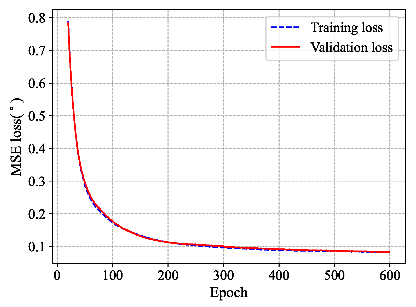
follows back-propagation towards minimizing the Mean Square Error(MSE) loss function as follows.
Ω ^ = a r g m i n Ω 1 I K i = 1 I h L , ( i ) θ ¯ ( i ) 2 2 ,
where 2 represents 2-norm, which measures the distance between the output vector of the network and the corresponding label, h L , ( i ) represents the output vector of the network corresponding to the i-th input vector. In the testing phase, the output vector of the output layer gives the estimated values of the DOAs of source signals explicitly.
For the lightweight DNN model, we define the size of the input vector by J ˜ = 2 ( M 1 ) . Note that with more layers and larger sizes of layers, the expressivity power of the network is increased during the training stage. However, the network tends to overfit the training data. As a result, in the testing stage, the performance is obviously degraded due to the lack of generalization. Furthermore, referring to [18], for the balance between the expressivity power with deeper network and aggravation with more network parameters, we set the number of hidden layers to be 2 and their sizes are equal to 2 3 J ˜ and 4 9 J ˜ , respectively, where x is equal to the largest integer not larger than x.

4.2. Construction of Training Data Set

Assuming that the searching angle range of the source signals is from θ m i n to θ m a x , the angular interval between two source signals in this range is defined as △, which is sampled from a set of [ m i n , m i n + d , m i n + 2 d , , m a x ] , where m i n , m a x , and d are the minimum angle interval between the DOAs of two source signals, the maximum angle interval, and an angle increment, respectively. In this way, any two source signals in this range that are spatially close to each other and those with large spacing can all be included in the training data set. Since the elements used as the input vector from the covariance matrix are not affected by the order of DOAs of source signals, with the DOA of the first source signal is sampled with a grid η from θ m i n to θ m a x ( K 1 ) , and the DOA of the k-th source signal is θ 1 + ( k 1 ) , k = 2 , , K . Furthermore, in order to adapt to the performance fluctuations in low SNRs, input vectors with multiple SNRs lower than 0dB are trained at the same time, making the lightweight DNN better adapted to unknown low and high SNRs during the testing phase.

4.3. Analysis of Number of Trainable Parameters

In this section, we present a comparative analysis of the proposed lightweight DNN, against the method in [25], the conventional DNN in [18], deep convolution network (DCN) in [19], and DeepMUSIC in [20], focusing on the number of trainable parameters. For the conventional DNN model in [18], we follow the setting in [18]. That is, for the autoencoder, we denote the size of each of the input and output layers as J = M ( M 1 ) , define the number of each encoder and decoder has one hidden layer with a size of J 2 , and define the number of spatial subregion as p. As a sequence, we obtain that for each of the multilayer classifiers after the autoencoder, the sizes of two hidden layers are equal to 2 3 J and 4 9 J , respectively. In addition, the size of output layer (denoted as γ ) for each multilayer classifier is equal to
γ = θ m a x θ m i n η p .
Correspondingly, according to the analysis in Section 3.1 for the proposed lightweight DNN, we have J ˜ = 2 M J . By following the above-mentioned definitions and the structure of the lightweight DNN, conventional DNN, and method in [25], we can obtain the number of parameters in the three fully connected DNN models, as shown in Table 1.
Table 2 shows the number of trainable parameters in DeepMUSIC and DCN by following the parameter settings in [19,20], which are mainly from the convolution layers and dense layers. For DeepMUSIC, C i n 1 represents the number of input channels, K s 1 is the kernel size of the first two convolution layers, and K s 2 is the kernel size of convolution layer 3 and convolution layer 4. N f is the number of filters. C o u t 1 and C o u t 2 represent the sizes of the first and second dense layers, respectively. For DCN, K s 3 , K s 4 , K s 5 and K s 6 represent the kernel size of the first till fourth convolution layers, of which the number of filters are N f 1 , N f 2 , N f 3 , and N f 4 , respectively. There is no dense layer.
When θ m i n = 60 , θ m a x = 60 , p = 6 , η = 1 , K = 2 , C i n 1 = 3 , C i n 2 = 2 , K s 1 = 5 , K s 2 = 3 , K s 3 = 25 , K s 4 = 15 , K s 5 = 5 , K s 6 = 3 , N f = 256 , N f 1 = 12 , N f 2 =6, N f 3 = 3 , N f 4 = 1 , C o u t 1 = 1024 , C o u t 2 = 120 
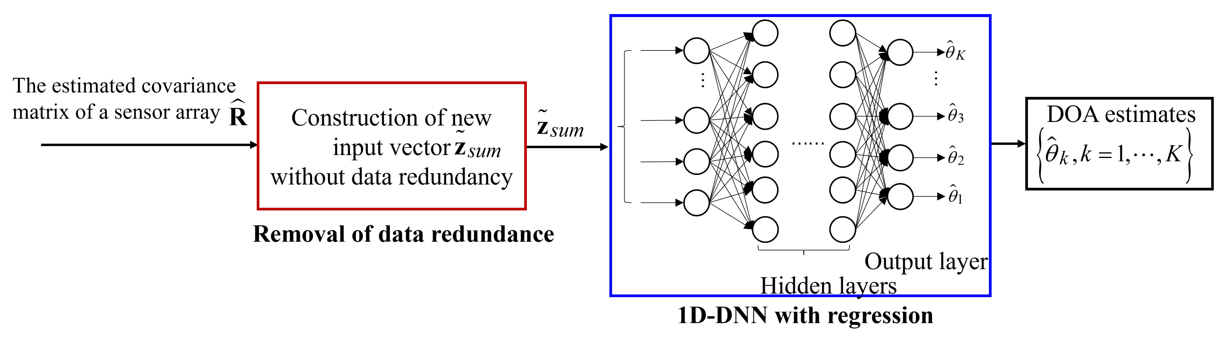
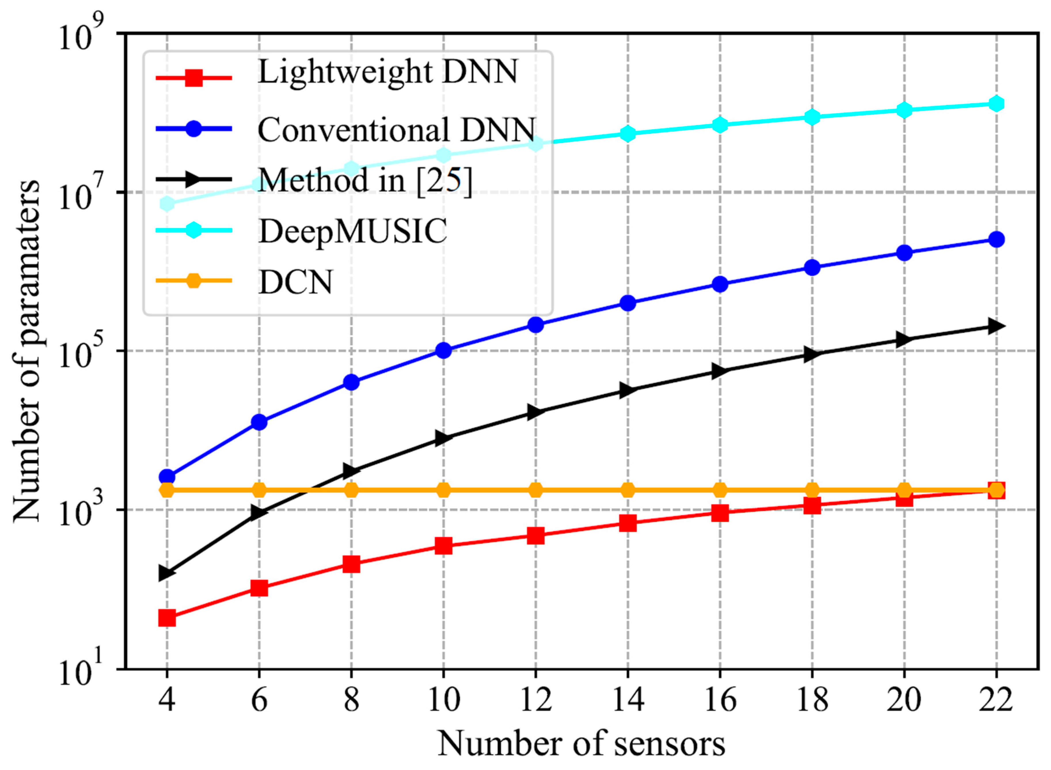
, the total parameters of the above-mentioned five deep learning methods versus the number of sensors are shown in Figure 2. From Figure 2, we can see that the number of trainable parameters in the lightweight DNN is significantly reduced compared to those of the conventional DNN, method in [25], and DeepMUSIC. In particular, when the number of sensors is 22, the number of parameters in the lightweight DNN is three orders, two orders, and five orders of magnitude less than that in the conventional DNN, the method in [25], and DeepMUSIC, respectively. This fact contributes to fitting the DNN-based DOA estimation into the embedded system. In addition, the lightweight DNN method has fewer parameters than the DCN method when the number of sensors is less than 22. The DCN method remains constant regardless of the number of sensors. This is because the input of the DCN method is the spatial spectrum proxy, which has a fixed length equal to θ m a x θ m i n η . On the other hand, the inputs of other methods are all explicitly relevant to the dimension of the array covariance matrix. Thus, their parameters are related to the number of sensors.

4.4. Analysis of Computational Complexity

Analogous to the approach detailed in [11], we quantify the primary computational complexity through the calculation of real-valued multiplications, as given in Table 3. In this table, L pertaining to the DCN denotes the length of the input vector, which is set as 120. In addition, we define
γ ˜ = θ m a x θ m i n η .
Note that when η = 0.1 and M = 22 , we have γ ˜ J > J ˜ > M > K [11] and ( M 1 ) ( M K ) ( M + 1 ) M J . According to the settings in Section 4.3, it is found from Table 3 that the computational complexity of the CBF, MUSIC, DeepMUSIC, and DCN methods is significantly higher than that of the fully-connected DNN-based methods, which corresponds to the testing time in Table 4 below.

5. Results

In this section, by conducting simulation experiments, the proposed lightweight DNN is compared with the conventional DNN [18], the method in [25], DeepMUSIC in [20] and DCN in [19] in terms of testing time and the root-mean-square-error (RMSE) of DOA estimation. In addition, the traditional spectrum-based methods such as MUSIC and CBF are also included for comparisons. Furthermore, the Cramér–Rao Bound (CRB) of DOA estimation [2] is given as a lower bound. The DNN models are implemented using TensorFlow as the backend. In the testing stage, for a fair comparison of testing time, all the above-mentioned methods are executed on the Intel(R) Core(TM) i7-8750H CPU at 2.20 GH.

5.1. Simulation Settings

Assuming that the ULA consists of 22 elements with an inter-element spacing equal to λ 2 . Supposing that there are two source signals impinging onto the array, of which the DOA range is from θ m i n = 60 to θ m a x = 60 . The angular interval between the DOAs of two source signals is from m i n = 2 to m a x = 40 , with d = 2 and η = 1 . The SNRs for different source signals are equal and S N R k is defined as the power ratio of the k-th source signal to noise in dB, which is given below.
S N R k = 10 l o g 10 σ s k 2 σ n 2 .
For the DNN models, in the training phase, the snapshots are set as 400. In addition, using input vectors from multiple SNRs of { 13 dB, 10 dB, 5 dB, 0 dB} to train the network simultaneously. Moreover, 10 groups of covariance vectors are collected for each direction setting with random noise. Therefore, ( 118 + 116 + + 80 ) × 4 × 10 = 79,200 input vectors are collected in the training dataset in total. The learning rate is μ = 0.001 and the mini-batch size is 32, the order of training data is shuffled in each epoch.

5.2. MSE Loss during Training and Validation

In this section, as given in Figure 3, we provide the training and validation MSE loss of the proposed lightweight DNN versus the number of epochs by randomly dividing the training data into 80 % for training and 20 % for validation. From Figure 3, we observe that the training loss and validation loss gradually reduce when the number of epochs increases and converges at about 400 epochs. Furthermore, they are close to each other. Therefore, we conclude that the proposed lightweight DNN with the input vector after the removal of data redundancy can accomplish the task of DOA estimation well. The detailed performance of DOA estimation in the testing stage is given as follows.

5.3. RMSE versus SNRs and Testing Time

In the testing phase, in order to verify the generalization of the DNN models, the noises and source signals are different from those that appeared in the training phase. In addition, the DOAs of sources are set to be non-integer (that is, off-grid), which does not appear in the training stage. The DOAs of source signals are ( θ 1 , θ 2 ) = ( 40.55 , 36.3 ) . The RMSE is used to measure the testing performance of different methods, defined as
R M S E = 1 G K g = 1 G k = 1 K | θ ^ k , g θ k | 2 ,
where G is the number of Monte Carlo simulation experiments, which is set as 200. K = 2. θ ^ k , g represents the DOA estimation value of the k-th source signal in the g-th experiment. In this part, SNR is taken from −16 dB to 10 dB with an interval of 2 dB and the number of snapshots is 400. The RMSE of DOAs estimated by the above-mentioned methods under different SNRs is given in Figure 4. Table 4 shows the averaged testing time for one trial. Figure 4 illustrates that the proposed lightweight DNN performs better than the method in [25], conventional DNN and the MUSIC and CBF methods with a grid of 1 . Its superiority is obvious when the SNR is lower than −8 dB. Moreover, the time spent by the lightweight DNN is about four times less than that spent by the MUSIC method with a grid of 1 . On the other hand, the proposed lightweight DNN has estimation accuracy lower than the MUSIC method with a grid of 0.1 . This is because the DNN-based approach yields biased estimators [20]. In contrast, the MUSIC method provides unbiased estimation when the source signals are uncorrelated and the number of arrays and snapshots is large [29,30]. It is noted that in Figure 4, the CBF method always fails because it suffers from the Rayleigh limit. In addition, the MUSIC method with a grid of 0.1 performs closely to the CRB when the SNR is larger than −8 dB. On the other hand, its performance deviates from the CRB when the SNR is larger than 5 dB. This phenomenon is caused by the limit of the searching grid in the MUSIC Method. Furthermore, as illustrated in Figure 4, the performance of the DeepMUSIC method is similar to that of the MUSIC method with a grid of 1 . This is because the label of the DeepMUSIC is the spatial spectrum of the MUSIC method and the grid in the DeepMUSIC method is equal to 1 to be consistent with the grid for other DNN methods. In addition, the DCN method performs better than the other methods except the lightweight DNN method, in most cases. In terms of testing time as given in Table 4, both DeepMUSIC and DCN methods cost much more than the lightweight DNN method.
It is noted that the higher estimation accuracy of the MUSIC method with a grid of 0.1 costs more spectrum searching load and the time it takes is about 25 times more than that by the lightweight DNN, as shown in Table 4. In addition, it is observed the time spent by the lightweight DNN is about 3 times less than that by the conventional DNN.

5.4. RMSE versus DOA Separations

In this part, the RMSE of different methods is shown with the variation of intervals between the DOAs of two source signals. The DOA of the first source signal is set to be 40.55 and the DOA of the second source signal is equal to 40.55 + Δ ˜ , where Δ ˜ is taken from the set of { 2.25 , 4.25 , 8.25 , , 32.25 , 36.25 } in sequence. The number of snapshots is 400. When SNR is −2 dB, the RMSE of DOA estimated by the above-mentioned methods under different DOA separations is shown in Figure 5. From Figure 5, it can be seen that the lightweight DNN performs better than the MUSIC method and CBF method when their searching grid is set to be 1 . Furthermore, it is always superior to the method in [25], conventional DNN method, DeepMUSIC method, and DCN method. Similar to the Figure 4, the MUSIC method with a grid of 0.1 approaches the CRB in most cases. However, it is noted that in a very small DOA separation such as 2.25 , even the MUSIC method with a grid of 0.1 fails. In contrast, the lightweight DNN performs well. In addition, it is shown that the CBF method with a grid of 0.1 gradually approaches the CRB when the DOA separation increases.

5.5. RMSE versus Number of Snapshots

In this part, the number of snapshots is selected from the set of {30, 50, 100, 200, 300, 400, 500, 600, 700, 900, 1200, 1500, 1800, 2000}, the DOAs of the two source signals are ( θ 1 , θ 2 ) = ( 40.55 , 36.3 ) . Figure 6 shows the RMSE of all methods against the number of snapshots when the SNR is equal to −2 dB. From Figure 6, it is found that except for the CBF method, the other methods perform better when the number of snapshots increases. In addition, it is observed that the DNN models trained in the scenario of 400 snapshots are applicable to the scenarios of more snapshots and fewer snapshots. Furthermore, the lightweight DNN behaves significantly better than the conventional DNN when the number of snapshots is less than 900. As the number of snapshots increases, the estimation accuracy of lightweight DNN is still slightly higher than that of the conventional DNN, method in [25], DeepMUSIC method, and DCN method. It is worth noting that the lightweight DNN is always superior to the MUSIC method with a grid of 1 and it performs better than the MUSIC method with 0.1 when the number of snapshots is less than 100.

5.6. RMSE versus Power Ratio of Two Source Signals

The DOAs of the two closely spaced source signals are ( θ 1 , θ 2 ) = ( 40.55 , 38.3 ) . The number of snapshots for both source signals is 400. The SNR for the first source signal is fixed as −2 dB. Figure 7 demonstrates the RMSE versus the power ratio of the second source signal to the first source signal. From Figure 7, we observe that the RMSE of the lightweight DNN method increases from 0.2 to about 1.5 when the power ratio of the second source signal to the first one increases from 1 to 14. Similarly, the RMSE of the conventional DNN, the method in [25], DeepMUSIC, and DCN methods increase slightly with the increment of the power ratio. As shown in Figure 7, the MUSIC and CBF methods always fail because the DOAs of source signals are very close. It is noted that the CRB reduces a bit when the power ratio increases. This is because the power of the second source signal is increased with the increment of the power ratio. However, the CRB is limited by the closely spaced source signals.

6. Discussion

From the analysis above, it can be seen that the number of total parameters in the lightweight DNN model is significantly reduced compared to those DNN models that use the upper triangular elements of the covariance matrix as input. In particular, when the number of sensors is 22, it is 2 and 3 orders of magnitude less than that in the conventional DNN model and the method in [25], respectively. This fact makes the proposed lightweight DNN suitable for real-time embedded applications. Furthermore, it is noted that the lightweight DNN can preserve high accuracy of DOA estimation and perform better than the conventional DNN and method in [
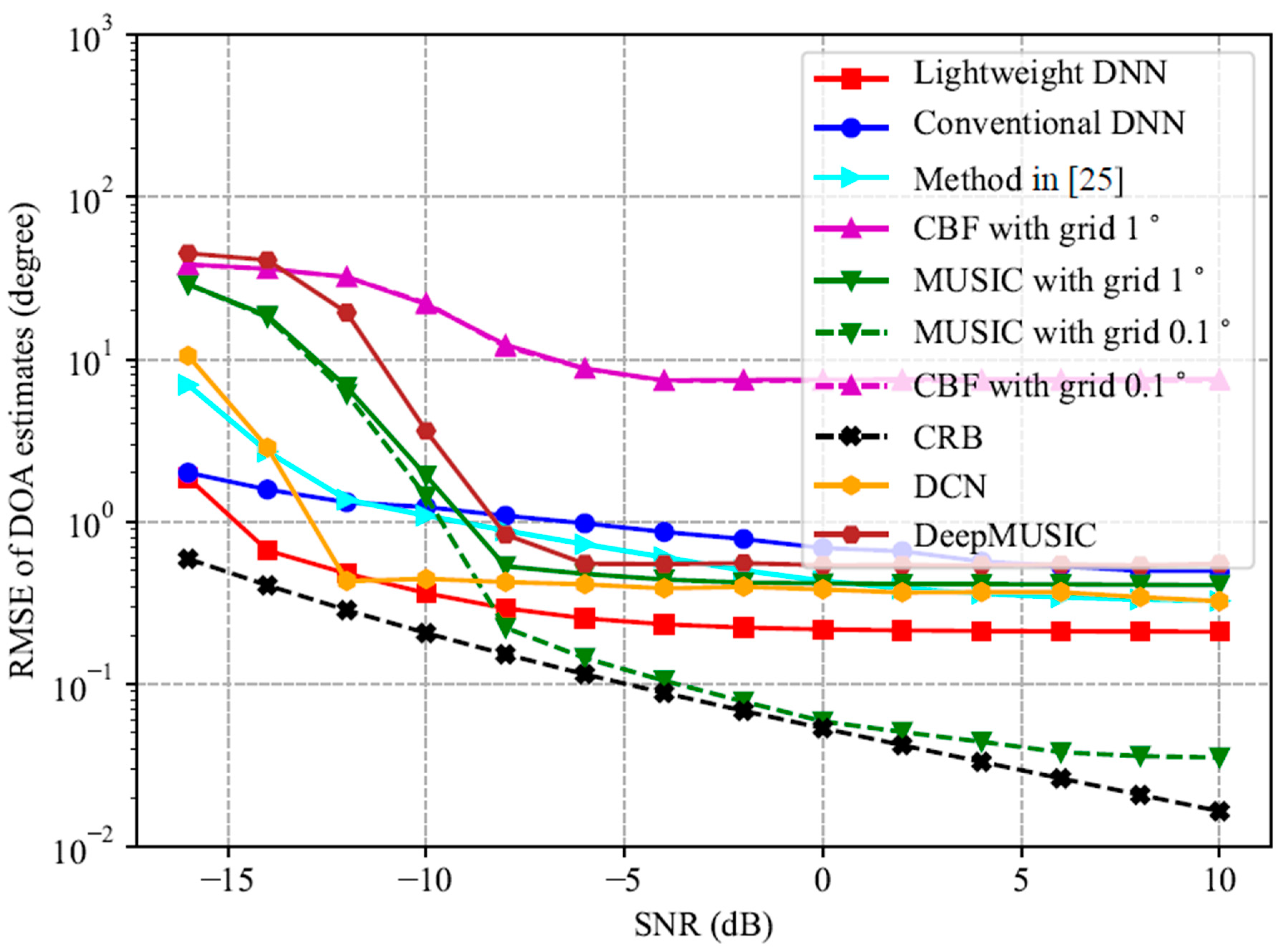
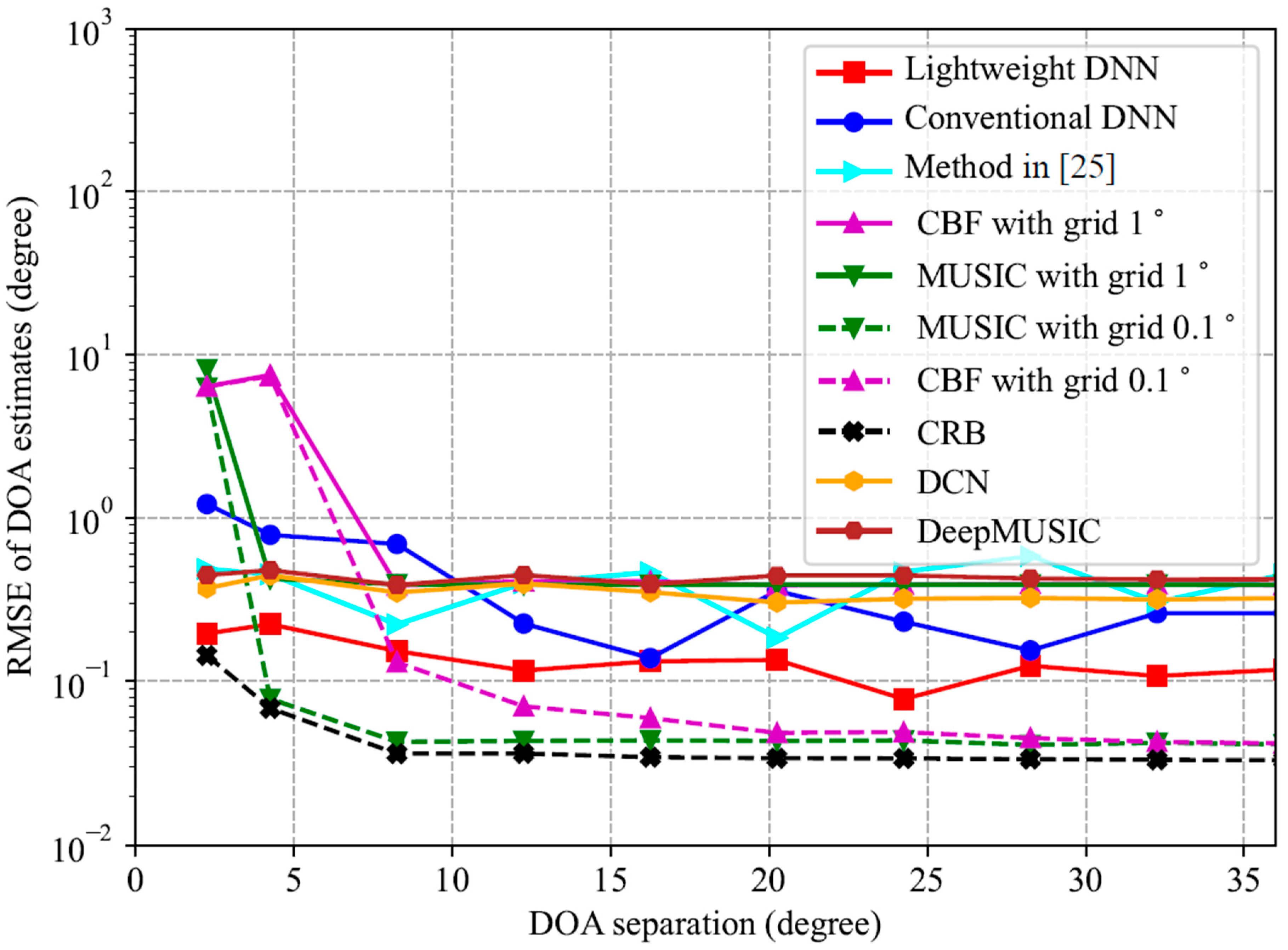
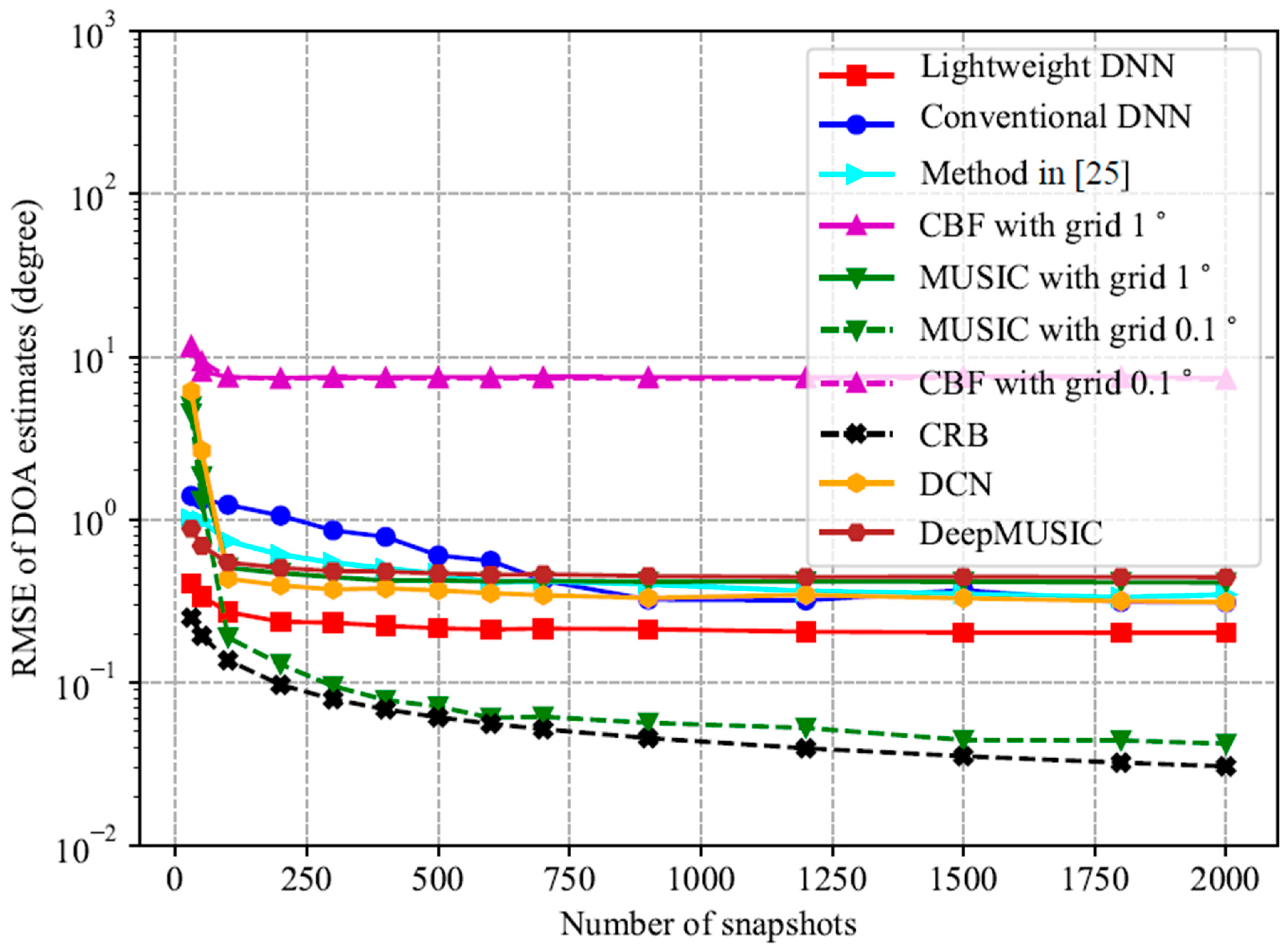
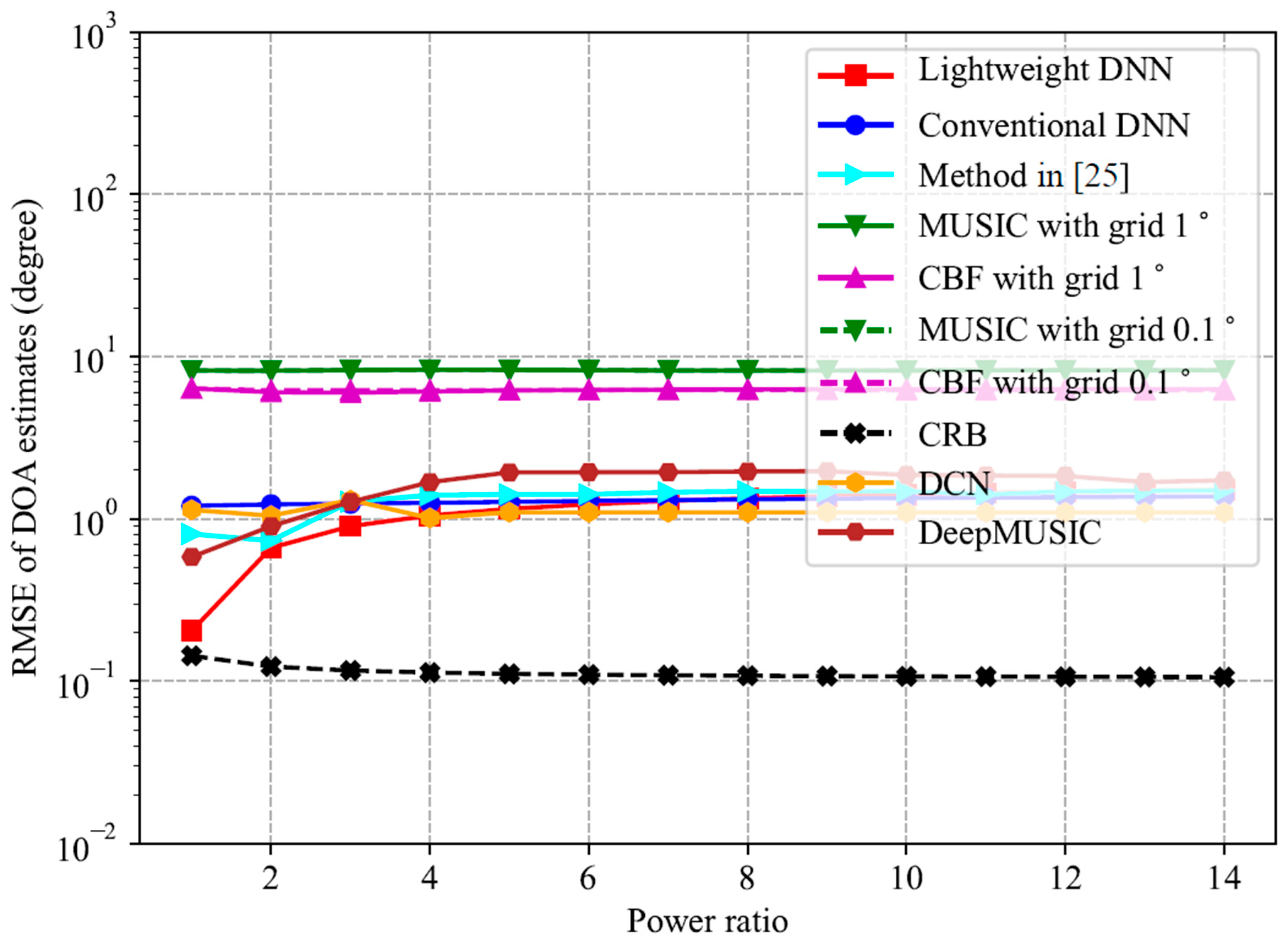
25]. In addition, it provides higher estimation accuracy and costs less trainable parameters and computational load than CNN-based methods such as DeepMUSIC and DCN. Also, it is illustrated that the lightweight DNN performs better than the spatial spectrum-based methods such as MUSIC and CBF method under harsh conditions such as low SNRs and/or closely spaced source signals and/or few snapshots. Moreover, its testing time is obviously shorter than that of the MUSIC and CBF method, due to the avoidance of spectrum searching and matrix decomposition. On the other hand, under good conditions such as high SNRs, the estimation accuracy of the lightweight DNN is lower than the MUSIC method with a grid of 0.1 . This is because the DNN-based methods are biased estimators while the MUSIC method can provide unbiased DOA estimation. It is noted that the MUSIC method with a grid of 0.1 provides higher estimation accuracy with a cost of a testing time of about 25 times more than that of the lightweight DNN. On the other hand, as shown in simulation results, the lightweight DNN can achieve high estimation accuracy such as 0.2 when the SNR is not extremely low (not lower than −6 dB) and the number of snapshots is not very small (not smaller than 100).

7. Conclusions

In order to make the DNN-based DOA estimation approaches real-time and less costly, we proposed a lightweight DNN model for a ULA. Compared to the conventional DNN model, the proposed lightweight DNN model has two improvements. Firstly, its input vector is designed by using the knowledge of ULA (that is, the steering vector of the ULA has the property of Vandermonde) to implement the removal of data redundancy as well as retain the DOA information. Therefore, the input vector is M 2 times less than the conventional DNN model, which contributes to reducing the sizes of the following hidden layers. Secondly, the output vector of the lightweight DNN model is designed in a regression fashion instead of classification, which has a size equal to the number of sources. Overall, the number of total parameters in the lightweight DNN model is significantly reduced compared to that in the existing DNN models. Furthermore, the lightweight DNN model performs better than the existing DNN models because the lightweight DNN model explores the characteristics of the signal received by the ULA for designing its input.

Author Contributions

Conceptualization and methodology, A.L., J.G. and Y.A.; software, validation, and visualization, J.G. and A.L.; formal analysis and investigation, J.G.; resources and data curation, A.L. and Z.L.; writing—original draft preparation and writing—review and editing, A.L., J.G. and Y.A.; supervision, A.L. and Z.L.; project administration, A.L.; funding acquisition, Y.A. All authors have read and agreed to the published version of the manuscript.

Funding

This work was supported in part by Natural Science Basic Research Program of Shaanxi Province, China (Program No. 2023-JC-YB-573), and in part by Basic Research Program of Taicang City, China, in 2023 (Program No. TC2023JC05), and in part by the Fundamental Research Funds for the Central Universities under Grants D5000210641 and G2022WD01022.

Data Availability Statement

Data are contained within the article.

Conflicts of Interest

The authors declare no conflicts of interest.

References

  1. Godara, L.C. Application of antenna arrays to mobile communications. II. Beam-forming and direction-of-arrival considerations. Proc. IEEE 1997, 85, 1195–1245. [Google Scholar] [CrossRef]
  2. Van Trees, H.L. Optimum Array Processing: Part IV of Detection, Estimation, and Modulation Theory; John Wiley & Sons: Hoboken, NJ, USA, 2002. [Google Scholar]
  3. Pesavento, M.; Trinh-Hoang, M.; Viberg, M. Three more decades in array signal processing research: An optimization and structure exploitation perspective. IEEE Signal Process. Mag. 2023, 40, 92–106. [Google Scholar] [CrossRef]
  4. Xiao, G.; Quan, Y.; Sun, Z.; Wen, B.; Liao, G. Design of a Digital Array Signal Processing System with Full Array Element. Remote Sens. 2023, 15, 4043. [Google Scholar] [CrossRef]
  5. Wen, F.; Shi, J.; Wang, X.; Wang, L. Angle estimation for MIMO radar in the presence of gain-phase errors with one instrumental Tx/Rx sensor: A theoretical and numerical study. Remote Sens. 2021, 13, 2964. [Google Scholar] [CrossRef]
  6. Capon, J. High-resolution frequency-wavenumber spectrum analysis. Proc. IEEE 1969, 57, 1408–1418. [Google Scholar] [CrossRef]
  7. Schmidt, R. Multiple emitter location and signal parameter estimation. IEEE Trans. Antennas Propag. 1986, 34, 276–280. [Google Scholar] [CrossRef]
  8. Roy, R.; Kailath, T. ESPRIT-estimation of signal parameters via rotational invariance techniques. IEEE Trans. Acoust. Speech Signal Process. 1986, 37, 984–995. [Google Scholar] [CrossRef]
  9. Haardt, M.; Nossek, J.A. Unitary ESPRIT: How to obtain increased estimation accuracy with a reduced computational burden. IEEE Trans. Signal Process. 1995, 43, 1232–1242. [Google Scholar] [CrossRef]
  10. Viberg, M.; Ottersten, B. Sensor array processing based on subspace fitting. IEEE Trans. Signal Process. 1991, 39, 1110–1121. [Google Scholar] [CrossRef]
  11. Yan, F.G.; Jin, M.; Liu, S.; Qiao, X.L. Real-valued MUSIC for efficient direction estimation with arbitrary array geometries. IEEE Trans. Signal Process. 2014, 62, 1548–1560. [Google Scholar] [CrossRef]
  12. Liu, A.; Liao, G. An eigenvector based method for estimating DOA and sensor gain-phase errors. Digit. Signal Process. 2018, 79, 116–124. [Google Scholar] [CrossRef]
  13. Tayem, N.; Kwon, H.M. Conjugate esprit (c-sprit). IEEE Trans. Trans. Antennas Propag. 2004, 52, 2618–2624. [Google Scholar] [CrossRef]
  14. Pastorino, M.; Randazzo, A. A smart antenna system for direction of arrival estimation based on a support vector regression. IEEE Trans. Antennas Propag. 2005, 53, 2161–2168. [Google Scholar] [CrossRef]
  15. El Zooghby, A.H.; Christodoulou, C.G.; Georgiopoulos, M. A neural network-based smart antenna for multiple source tracking. IEEE Trans. Antennas Propag. 2000, 48, 768–776. [Google Scholar] [CrossRef]
  16. Randazzo, A.; Abou-Khousa, M.A.; Pastorino, M.; Zoughi, R. Direction of arrival estimation based on support vector regression: Experimental validation and comparison with MUSIC. IEEE Antennas Wirel. Propag. Lett. 2007, 6, 379–382. [Google Scholar] [CrossRef]
  17. Xiao, X.; Zhao, S.; Zhong, X.; Jones, D.L.; Chng, E.S.; Li, H. A learning-based approach to direction of arrival estimation in noisy and reverberant environments. In Proceedings of the 2015 IEEE International Conference on Acoustics, Speech and Signal Processing (ICASSP), South Brisbane, Australia, 6 August 2015; pp. 2814–2818. [Google Scholar]
  18. Liu, Z.M.; Zhang, C.; Philip, S.Y. Direction-of-arrival estimation based on deep neural networks with robustness to array imperfections. IEEE Trans. Antennas Propag. 2016, 66, 7315–7327. [Google Scholar] [CrossRef]
  19. Wu, L.; Liu, Z.M.; Huang, Z.T. Deep convolution network for direction of arrival estimation with sparse prior. IEEE Signal Process. Lett. 2019, 26, 1688–1692. [Google Scholar] [CrossRef]
  20. Elbir, A.M. DeepMUSIC: Multiple signal classification via deep learning. IEEE Sens. Lett. 2020, 4, 1–4. [Google Scholar] [CrossRef]
  21. Papageorgiou, G.K.; Sellathurai, M.; Eldar, Y.C. Deep networks for direction-of-arrival estimation in low SNR. IEEE Trans. Signal Process. 2021, 69, 3714–3729. [Google Scholar] [CrossRef]
  22. Labbaf, N.; Oskouei, H.D.; Abedi, M.R. Robust DoA estimation in a uniform circular array antenna with errors and unknown parameters using Deep Learning. IEEE Trans. Green Commun. Netw. 2023, 7, 2143–2152. [Google Scholar] [CrossRef]
  23. Ping, Z. DOA estimation method based on neural network. In Proceedings of the 2015 10th International Conference on P2P, Parallel, Grid, Cloud and Internet Computing (3PGCIC), Krakow, Poland, 4–6 November 2015; pp. 828–831. [Google Scholar]
  24. Agatonovic, M.; Stankovic, Z.; Milovanovic, I.; Doncov, N.; Sit, L.; Zwick, T.; Milovanovic, B. Efficient neural network approach for 2D DOA estimation based on antenna array measurements. Prog. Electromagn. Res. 2013, 137, 741–758. [Google Scholar] [CrossRef]
  25. Xiong, Y.; Liu, A.; Gao, X.; Yauhen, A. DOA Estimation Using Deep Neural Network with Regression. In Proceedings of the 2022 5th International Conference on Information Communication and Signal Processing (ICICSP), Shenzhen, China, 26–28 November 2022; pp. 1–5. [Google Scholar]
  26. Zhou, C.; Gu, Y.; Fan, X.; Shi, Z.; Mao, G.; Zhang, Y.D. Direction-of-arrival estimation for coprime array via virtual array interpolation. IEEE Trans. Signal Process. 2018, 66, 5956–5971. [Google Scholar] [CrossRef]
  27. Reed, I.S.; Mallett, J.D.; Brennan, L.E. Rapid convergence rate in adaptive arrays. IEEE Trans. Aerosp. Electron. Syst. 1974, 10, 853–863. [Google Scholar] [CrossRef]
  28. Wax, M.; Kailath, T. Detection of signals by information theoretic criteria. IEEE Trans. Acoust. Speech Signal Process. 1985, 33, 387–392. [Google Scholar] [CrossRef]
  29. Stoica, P.; Nehorai, A. MUSIC, maximum likelihood, and Cramer-Rao bound. IEEE Trans. Acoust. Speech Signal Process. 1989, 37, 720–741. [Google Scholar] [CrossRef]
  30. Li, F.; Liu, H.; Vaccaro, R.J. Performance analysis for DOA estimation algorithms: Unification, simplification, and observations. IEEE Trans. Aerosp. Electron. Syst. 1993, 29, 1170–1184. [Google Scholar] [CrossRef]
Figure 1. Proposed lightweight DNN for DOA estimation in a ULA array.
Remotesensing 16 01423 g001
Figure 2. Trainable parameters in the DNN models versus number of sensors.
Remotesensing 16 01423 g002
Figure 3. MSE loss versus epoch given by the proposed lightweight DNN.
Remotesensing 16 01423 g003
Figure 4. RMSE versus SNR when ( θ 1 , θ 2 ) = ( 40.55 , 36.3 ) .
Remotesensing 16 01423 g004
Figure 5. RMSE versus DOA separation when SNR = −2 dB.
Remotesensing 16 01423 g005
Figure 6. RMSE versus number of snapshots when SNR = −2 dB.
Remotesensing 16 01423 g006
Figure 7. RMSE versus power ratio of second source signal to the first one when ( θ 1 , θ 2 ) = ( 40.55 , 38.3 ) .
Remotesensing 16 01423 g007
Table 1. Analysis of number of trainable parameters in fully-connected DNN methods.
Number of ParametersAutoencoderHidden Layer 1Hidden Layer 2Output Layer
Lightweight DNNN.A. ( J ˜ + 1 ) × 2 3 J ˜ ( 2 3 J ˜ + 1 ) × 4 9 J ˜ ( 4 9 J ˜ + 1 ) × K
Method in [25]N.A. ( J + 1 ) × 2 3 J ( 2 3 J + 1 ) × 4 9 J ( 4 9 J + 1 ) × K
Conventional DNN ( J + 1 ) × J 2 + ( J 2 + 1 ) × J × p ( J + 1 ) × 2 3 J × p ( 2 3 J + 1 ) × 4 9 J × p ( 4 9 J + 1 ) × γ × p
Table 2. Analysis of number of trainable parameters in CNN-based methods.
Number of ParametersConvolution Layer 1Convolution Layer 2Convolution Layer 3Convolution Layer 4Dense Layer 1Dense Layer 2
DeepMUSIC K s 1 2 × C i n 1 × N f K s 1 2 × N f × N f K s 2 2 × N f × N f K s 2 2 × N f × N f M 2 × N f × C o u t 1 C o u t 1 × C o u t 2
DCN K s 3 × C i n 2 × N f 1 K s 4 × N f 1 × N f 2 K s 5 × N f 2 × N f 3 K s 6 × N f 3 × N f 4 N.A.N.A.
Table 3. Analysis of primary computational complexity.
AlgorithmsPrimary Computational Complexity
Lightweight DNN O [ J ˜ × 2 3 J ˜ + 2 3 J ˜ × 4 9 J ˜ + 4 9 J ˜ × K ]
Method in [25] O [ J × 2 3 J + 2 3 J × 4 9 J + 4 9 J × K ]
Conventional DNN O [ J × J 2 + J 2 × J × p + J × 2 3 J × p + 2 3 J × 4 9 J × p + 4 9 J × γ × p ]
MUSIC 4 × O [ ( M + 1 ) ( M K ) γ ˜ + M 2 K ]
CBF 4 × O [ ( M + 1 ) M γ ˜ ]
DeepMUSIC O [ K s 1 2 × C i n 1 × N f × M 2 + K s 1 2 × N f × N f × M 2 + K s 2 2 × N f × N f × M 2 × 2 + M 2 × N f × C o u t 1 + C o u t 1 × C o u t 2 ]
DCN O [ K s 3 × C i n 2 × N f 1 × L + K s 4 × N f 1 × N f 2 × L + K s 5 × N f 2 × N f 3 × L + K s 6 × N f 3 × N f 4 × L ]
Table 4. Averaged testing time for one trial.
MethodLight Weight DNNMethod in [25]Conventional DNNMUSIC with Gird 1 CBF with Grid 1 MUSIC with Gird 0.1 CBF with Grid 0.1 Deep MUSICDCN
Testing time/ms0.91.13.33.72.322.917.926.320.4
Disclaimer/Publisher’s Note: The statements, opinions and data contained in all publications are solely those of the individual author(s) and contributor(s) and not of MDPI and/or the editor(s). MDPI and/or the editor(s) disclaim responsibility for any injury to people or property resulting from any ideas, methods, instructions or products referred to in the content.

