Abstract
The aim of this paper is to assess the correlation of groundwater level changes (or groundwater level anomalies (GWLA)) obtained from direct measurements in wells with groundwater storage anomalies (GWSA) calculated using Gravity Recovery and Climate Experiment (GRACE) products and Global Land Data Assimilation Systems (GLDAS) models across different climate zones, from temperate Poland to Arctic Sweden. We recognize that such validation studies are needed to increase the understanding of the spatio-temporal limits of remote sensing model applicability, not least in data-scarce sub-Arctic and Arctic environments where processes are complex due to the impacts of snow and (perma) frost. Results for temperate climates in Poland and southern Sweden show that, whereas one of the models (JPL_NOAH_GWSA) failed due to water balance term overestimation, the other model (CSR_CLM_GWSA) produced excellent results of monthly groundwater dynamics when compared with the observations in 387 groundwater wells in the region during 2003–2022 (cross-correlation coefficient of 0.8). However, for the sub-Arctic and Arctic northern Sweden, the model suitable for other regions failed to reproduce typical northern groundwater regimes (of the region’s 85 wells), where winter levels decrease due to the blocking effect of ground frost on groundwater recharge. This suggests, more generally, that conventional methods for deriving GWSA and its seasonality ceases to be reliable in the presence of considerably infiltration-blocking ground frost and permafrost (whereas snow storage modules perform well), which hence need further attention in future research. Regarding long-term groundwater level trends, remote sensing results for southern Sweden show increasing levels, in contrast with observed unchanged to decreasing (~10 mm/a) levels, which may not necessarily be due to errors in the remote sensing model but may rather emphasize impacts of anthropogenic pressures, which are higher near the observation wells that are often located in eskers used for water supply. For sub-Arctic and Arctic Sweden, the (relatively uncertain) trend of the remote sensing results nevertheless agrees reasonably well with the groundwater well observations that show increasing groundwater levels of up to ~14 mm/a, which, e.g., is consistent with reported trends of large Siberian river basins.
1. Introduction
Groundwater is currently the most important source of water consumption and economic development [1]. Therefore, continuous monitoring of changes in its storage, quality and use is essential, especially in the context of climate change and land use change, including agricultural expansion. Recent years have witnessed a noticeable decline in the availability of groundwater resources in many regions of the world, which were largely related to changes in climate, land use and overconsumption of groundwater supplies [2,3].
To monitor groundwater resources, observation wells are used for direct measurement of both groundwater levels and quality. An intensive network of wells enhances the accuracy and representativeness of water resource assessment within a surveyed area. Nonetheless, drilled wells can be expensive and labour-intensive, and the data collection is limited to specific points. Additionally, in some locations, measurements are either not feasible (e.g., in remote or inaccessible areas) or their results are unreliable (e.g., where groundwater level fluctuations are affected by human activities) [4].
Thanks to the Gravity Recovery and Climate Experiment (GRACE) and its successor GRACE Follow On (GRACE-FO), it has been possible to collect monthly data on globally distributed total water storage (TWS) anomalies for more than 20 years [5,6,7]. GRACE is a joint mission between the National Aeronautics and Space Administration (NASA) and Deutsches Zentrum für Luft-und Raumfahrt (DLR). It started in March 2002 and ended in October 2017. Then, in May 2018, the GRACE Follow-On mission was launched as a joint effort between NASA and GeoForschungsZentrum (GFZ). The difference between GRACE-FO and GRACE is the utilization of more advanced measuring instrumentations, such as laser interferometry. The temporal resolution of the GRACE products is approximately one month [8]. The working principle involves measuring a slight distance variation between two GRACE satellites, which makes it possible to infer the gravity changes. The measurements provide a basis for deriving changes in TWS (TWSA), which can then be converted into changes in groundwater storage [9] by subtracting the changes of other water compartments from TWSA. The TWSA offers valuable insights into critical water cycle characteristics, both spatially and temporally, including monthly to multi-annual water surpluses or deficits [10,11].
The Global Land Data Assimilation System (GLDAS) is a joint project between NASA and the National Oceanic and Atmospheric Administration (NOAA). The GLDAS model integrates satellite and ground observations, generating four land surface sub-models (NOAH, VIC, CLM, MOSAIC). Among these, the NOAH model is recommended in many studies that have focused on analysing water storage changes [12]. Many models ignore ex-soil water–groundwater change, which is unrealistic. It is also common to use simplified representations that describe only the vertical flow of water. In the NOAH model, using well observations of groundwater level, the influence of lateral flow is also assessed [9,13,14]. We selected NOAH and CLM models for this research. NOAH was selected because it is recommended in the NASA user handbook (GRACE L-3 Product User Handbook, GRACE D-103133, NASA-JPL, 10 January 2019) for GWS analyses. On the other hand, in the CLM model, ready-made calculations of GWS can be found from 2019.
The use of modern satellite missions and climatic or assimilation models to determine the storage or level of groundwater has been of interest to scientists for a long time. The approach has yielded novel insights into the storage dynamics of very large areas. It has also enhanced our understanding of regions that show large fluctuations or changes [15,16,17]. Currently, increasing interest is being seen in assessments at finer scales, focusing on individual countries, states, rivers and basins of various sizes, e.g., [4,7,18,19,20]. In many cases, such remote sensing assessments can overcome problems related to the traditional observation well data, including severe spatio-temporal data gaps, which in many cases are due to the underdevelopment of long-term regional and national groundwater monitoring programs [21,22,23,24], the unavailability of local to regional data, and uncertainties in status and configuration of the wells. Such problems are particularly pronounced in high latitude and Arctic regions, characterized by sparse populations, above-average temperature increases, declining water quality, and by a pivotal role in the global carbon cycle [25,26,27].
While remote sensing studies have documented variations in groundwater storage across the Arctic, including vast regions in Russia and North America (e.g., [28,29,30]), there remain open questions regarding the accuracy of local to regional groundwater storage (GWS) results obtained from the GRACE observations and GLDAS models in the Arctic and other regions. Challenges have previously been identified in obtaining robust correlations between groundwater levels in wells and GWS results in the GRACE and GLDAS models for Poland [7]. Recent efforts have been focused on enhancing downscaling schemes (e.g., [31]). Compared with previous studies of Poland [4,7], the considered time period of this study was significantly extended. To the best of our knowledge, validation studies of groundwater storage anomalies, calculated using GRACE observations and GLDAS model output, are lacking for Sweden and for most regions that have permafrost or extended periods of ground frost, including the Arctic. Moreover, we here consider recently published ready-made GWSA products related to the GLDAS CLM model, referred to as CSR_CLM_GWSA (see Section 4 and http://disc.gsfc.nasa.gov, accessed 28 April 2024). The aim of this paper is to assess correlations between monthly groundwater level changes obtained from direct well measurements and GWS calculated from GRACE observations and GLDAS model output, considering a long-term (multi-decadal) time scale, and multiple climate zones spanning spatially from southern Poland to the Arctic region in Sweden. More specifically, the research aims to enhance the understanding of differences (if any) in the accuracy of GWS change predictions obtained from the GRACE/GLDAS combination under different (hydro-climatic) conditions. This could help identify the limits of their reliable applicability and possible enhancement needs. Furthermore, we aim to enhance our understanding of the expected changes in groundwater storage regimes within the studied regions (located in tempered and partly polar climate zones) [32,33], which holds significant implications for groundwater use strategies (IVL, 2020; Polish HydroGeological Institute National Research Institute, 30 October 2023).
2. Study Area Description
This article analyses five areas, comprising Poland and four areas that together cover Sweden. Poland is located in central Europe, extending approximately from 14°E to 24°E and from 49°N to 55°N (Figure 1a). Its total area is 322,575 km2, of which 311,888 km2 (about 97%) is land area (including inland waters). Almost the entire area of Poland falls within two main river basins: the Vistula river basin (194,500 km2) and the Oder river basin (118,900 km2). The two basins divide Poland into eastern and western parts, while the different climate zones are instead arranged in latitudinal zones: mountains with more rainfall in the south and the influence of the Baltic Sea with lower annual temperature amplitudes in the north. The effective porosity coefficient estimated for Poland is similar in the Vistula and Oder basins, with a value of about 0.25. Poland is mostly a lowland country, so the climate in its area is relatively uniform. Groundwater level fluctuations in Poland, obtained in previous studies based on GRACE and GLDAS data [14,34], do not differ practically in the areas of both the basins; therefore, in this article, the whole territory of Poland appears as one uniform region. According to the Köppen classification system, the predominant climate in Poland is temperate, without a dry season but with warm summers (abbreviated Cfb in the Köppen classification, [35,36].
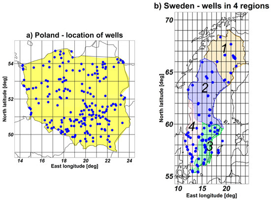
Figure 1.
The spatial extent of (a) Poland (here treated as one region), including the location of the available 215 groundwater wells, and (b) Sweden (divided into four regions of different hydroclimate, excluding Gotland), including the location of the available 257 wells (42, 43, 113 and 59 for regions 1, 2, 3 and 4 respectively). Please note that the maps are shown at different scales and that some wells overlap.
Sweden is located in northern Europe (on the eastern Scandinavian peninsula) and stretches approximately between 11° and 24° E and 55° and 69°N. The total land area of Sweden is around 530,000 km2, and it consists of 119 coastal catchment areas larger than 200 km2 (SMHI, 2023, https://www.smhi.se/kunskapsbanken/hydrologi/avrinningsomraden, accessed 28 April 2024). There are various types of groundwater aquifers in Sweden, ranging from (1) extensive aquifers in large eskers (gravel and sand) to (2) aquifers in (till) soils and fractured rock that include local (“small”) systems (SGU; 2015; SGU—Sveriges geologiska Undersokning, in Eng.: Geological Survey of Sweden). The GWS changes in some of the small aquifers caused by rainfall or snowmelt events occur with weekly or even monthly delays, unlike the quick responses seen in some esker systems [32]. Due to the difference in climate conditions across Sweden (from temperate in the south to polar and subarctic in the north) and the related hydrological regimes, the country-specific analysis for Sweden is carried out in four different research regions (excluding Gotland, Figure 1b):
- Region 1—north of the Umeälven basin, where the GWS regime mainly depends on snowmelt events in late spring. The predominant climate according to the Köppen classification system is cold (sub-)Arctic, without a dry season and with cold summers (abbreviated Dfc, [36,37].
- Region 2—between the Umeälven and Dalälven basins, where the GWS regime is still strongly governed by snowmelt in spring and autumn rainfall. According to the Köppen classification system, the predominant climate is the same as for region 1.
- Region 3—the eastern region south of Dalälven basin, where the GWS regime is governed by rainfall of the autumn–winter period and spring snowmelt. According to the Köppen classification system, the predominant climate is temperate, without a dry season and with warm summers (abbreviated Cfb, [36,37]). The region additionally has significantly lower annual average precipitation (around 600 mm/year) than region 4.
- Region 4—the western region south of Dalälven basin, where the GWS regime is mainly governed by autumn–winter rainfalls, as well as the, negligible, effect of snowmelt. According to the Köppen classification system, the predominant climate is the same as in region 3 (also as in Poland). The region additionally has significantly higher annual average precipitation (around 900 mm/year) than region 3.
Similar divisions appear in SGU’s classification of regimes of quick groundwater aquifers in Sweden, which is based on groundwater level analysis [32] and SMHI’s districts for natural hydrological regimes. In northern Sweden, there is also significant water storage in hydropower dams. We assessed the potential impact of surface water storage in hydropower dams by blocking out the grid cells in and around the reservoirs and recalculating the regional GWSA values. The assessment, however, showed that the derived regional average GWSA results were not significantly impacted by reservoir storage, and, as a result, we did not pursue this line of investigation further (Figure A1—Appendix A).
3. Observational Data and Models
3.1. GRACE Observations
GRACE and GRACE-FO data were downloaded from the Jet Propulsion Laboratory (JPL) website as a solution obtained using the MASCON approach [38,39]. The dataset contains gridded (0.5°) monthly global total water storage anomalies (TWSA) computed relative to a time mean (epochs 2004.000 to 2009.999), shown in the height of the total water storage. MASCON, or spherical cap mass concentration, differs from traditional spherical harmonic gravity solutions. MASCON grids do not need to be destriped or smoothed. During post-processing at JPL, the Coastal Resolution Improvement (CRI) filter was applied [17] to make the data suitable for ocean, ice, and land hydrological analyses. The data are available in netCDF format at https://grace.jpl.nasa.gov/data/get-data/jpl_global_mascons/, accessed 28 April 2024.
Monthly TWSA solutions for Poland and Sweden were downloaded for the period from 16 April 2002 to 16 July 2022. Accounting for the temporal gap between GRACE and GRACE-FO missions, a total of 244 monthly epochs with TWS data were obtained. We did not deal with the gap, as it does not affect the final results. From the global dataset, grid points located within the borders of Poland (168 grid cells) and Sweden (318 grids in total, with 99, 121, 51 and 47 for areas 1, 2, 3 and 4, respectively) were taken. The above TWSA data were used to calculate groundwater storage anomaly (GWSA), incorporating complementary data from the GLDAS model (see Section 3.3 and Section 4).
3.2. Observations in Groundwater Wells
In this study, monthly observations in Poland were collected for the period from November 2006 to October 2021 from the “Hydrogeological Bulletins,” published annually. The Polish groundwater monitoring network consists of over one thousand stations, from which 215 were used for computations (only those with continuous time series during the research period). The location of wells in Poland is presented in Figure 1a [34]. For Sweden, monthly well observations were obtained from SGU (2023), https://www.sgu.se/grundvatten/grundvattennivaer/matstationer/, accessed 28 April 2024. The groundwater monitoring network in Sweden consists of 271 stations, from which 259 were used for analysis (again, only those with continuous time series during the research period). Localization of wells across Sweden is presented in Figure 1b.
3.3. The GLDAS NOAH Model
Monthly gridded GLDAS data from the NOAH model (v3.3) is available at the NASA JPL website (https://podaac.jpl.nasa.gov/dataset/TELLUS_GLDAS-NOAH-3.3_TWS-ANOMALY_MONTHLY, accessed 28 April 2024). The data had already been post-processed, comprising the following variables: snow water equivalent (SWE), soil moisture (SM) content (for depths from 0 to 200 cm) and plant canopy surface water content (approximated as the biomass (BM), all expressed in kg/m2, convertible to the units of length (height) by accounting for the density. It should be emphasized that the GLDAS data do not include estimates related to groundwater storage. The data are available in the net_CDF format as separate files for each month, with a 1° resolution synchronized with the GRACE/GRACE FO data. Global data were downloaded for the period from April 2002 to October 2022, with specific data for Poland and Sweden extracted from the global data. The above data were used to calculate ground water storage anomaly (GWSA) by combining TWS data from the GRACE/GRACE FO.
3.4. The GLDAS CLM Model
Additionally, we considered the CLM model within the GLDAS model system for comparative purposes. This model provides ready-to-use GWS calculations in equivalent water height (mm) with a resolution of 0.25°. The GWS data within this model are computed using the same methodology as our computations from GRACE JPL and NOAH (see Equation (1)). The total terrestrial water anomaly observation from Gravity Recovery and Climate Experiment (GRACE) was assimilated to the CLM model in 2019 [40]. The GRACE RL06 and GRACE Follow-On data were provided by the Center for Space Research at the University of Texas [35].
These data were published in 2019 but were recalculated and cover the entire GRACE/GRACE-FO availability period (from April 2002 to the present). The data format is netCDF, with one global data file per month, available at https://hydro1.gesdisc.eosdis.nasa.gov/data/GLDAS/GLDAS_CLSM025_DA1_D.2.2/, accessed 28 April 2024. At this resolution, there were 657 grid cells in Poland and 1295 grid cells in Sweden (409, 489, 203, and 194 for regions 1, 2, 3 and 4, respectively).
4. Theory
The main components of the total water storage anomaly (TWSA) are the groundwater storage (GWS), the soil moisture (SM), the snow water equivalent (SWE) and the biomass of plant canopy (BM). Using GRACE observations, it is possible to obtain the TWS, which were computed relative to a time mean of their standard period (2004.000 to 2009.999). Related SM, SWE and BM estimates can be acquired from the GLDAS models. To ensure that all data are compatible, anomalies are computed by subtraction mean values calculated for the same standard period used in GRACE, yielding TWSA, SMA, SWEA and BMA.
Using the anomalies of GRACE and GLDAS data, the anomalies of the groundwater storage (GWSA) can be separated from the TWSA without taking into account surface water storage (SWS), previously described in [41,42] and in the JPL header file (https://podaac.jpl.nasa.gov, accessed 28 April 2024). The authors’ previous research [4] shows the limited impact of SWS on the final GWSA result. Surface water constitutes approximately 1.5% of Poland’s area (https://en.wikipedia.org/wiki/Geography_of_Poland, accessed 28 April 2024). Data for SWS were obtained from https://gravis.gfz-potsdam.de/, accessed 28 April 2024. Average SWS for the Vistula and Oder basin areas were calculated. The time series obtained are presented in Figure A2, Appendix A, showing that they constitute a small part of the GWSA value (amplitudes for well values are approx. 1 m, for CSR_CLM_GWS approx. 25 cm, for JPL_NOAH_GWS approx. 20 cm, and for SWS approx. 14 mm). The inclusion of SWS will not change the conclusion of this article and, therefore, is not considered in this study (Equation (1)).
where is groundwater storage anomaly, is total water storage anomaly, is soil moisture anomaly, is snow water equivalence anomaly, and is biomass component anomaly.
The obtained values of changes in groundwater were averaged over the five analysed areas (the entire area of Poland and four regions of Sweden). The GWSA anomalies obtained in this way were denoted as JPL_NOAH_GWSA.
In the GLDAS CLM model, GRACE data were obtained from the CSR computing centre, and the total water content in soil, snow, and plants was modelled to obtain GWSA. After averaging the values obtained from this model over the same five studied regions, we obtain the average GWSA, denoted as CSR_CLM_GWSA.
The results of direct measurements (WELL_GWLA) from wells were processed similarly, i.e., their anomalies were calculated and averaged over the considered time period (16 April 2002 to 16 July 2022). All datasets were harmonized using linear approximation to the same dates (the middle of a given month). Subsequently, we analysed the consistency between these three datasets of estimated average groundwater level anomalies. This included investigating potential systematic differences, such as differences in amplitudes as well as time cross-correlation functions (CCF) between paired datasets (WELL_GWLA versus CSR_CLM_GWS and WELL_GWLA versus JPL_NOAH_GWSA).
In summary, we derived and calculated three indicators describing changes in groundwater content within the given areas: (1) the changes in water levels in wells (WELL_GWL), (2) the average groundwater storage anomaly (GWSA) calculated based on GRACE TWS (processed at JPL) plus the GLDAS NOAH model (JPL_NOAH_GWSA), and (3) GWSA obtained from GRACE TWS (processed at CSR) plus the GLDAS CLM model (CSR_CLM_GWSA). The computation models differ in their resolutions, as follows: GRACE JPL data are given on a grid of 0.5 degrees, CSR_CLM_GWSA is given every 0.25 degrees, and NOAH product is given at the resolution of 1 degree. The data from all of the models were averaged over all cells within each of the five regions (Poland and four separate regions in Sweden). It was assumed that the quality of averages calculated over a fairly large area is independent of the initial resolution of the representation of a given quantity. The same principle applies to wells.
The calculations of trend performed in the paper, take advantage of a simple model with simultaneous determination of the trend and seasonal components, using the model [43], as follows:
where is the annual frequency and is the time in days, the coefficients were determined on the basis of linear regression using the least squares method. The coefficients fulfil the role of trend.
5. Results
5.1. Poland
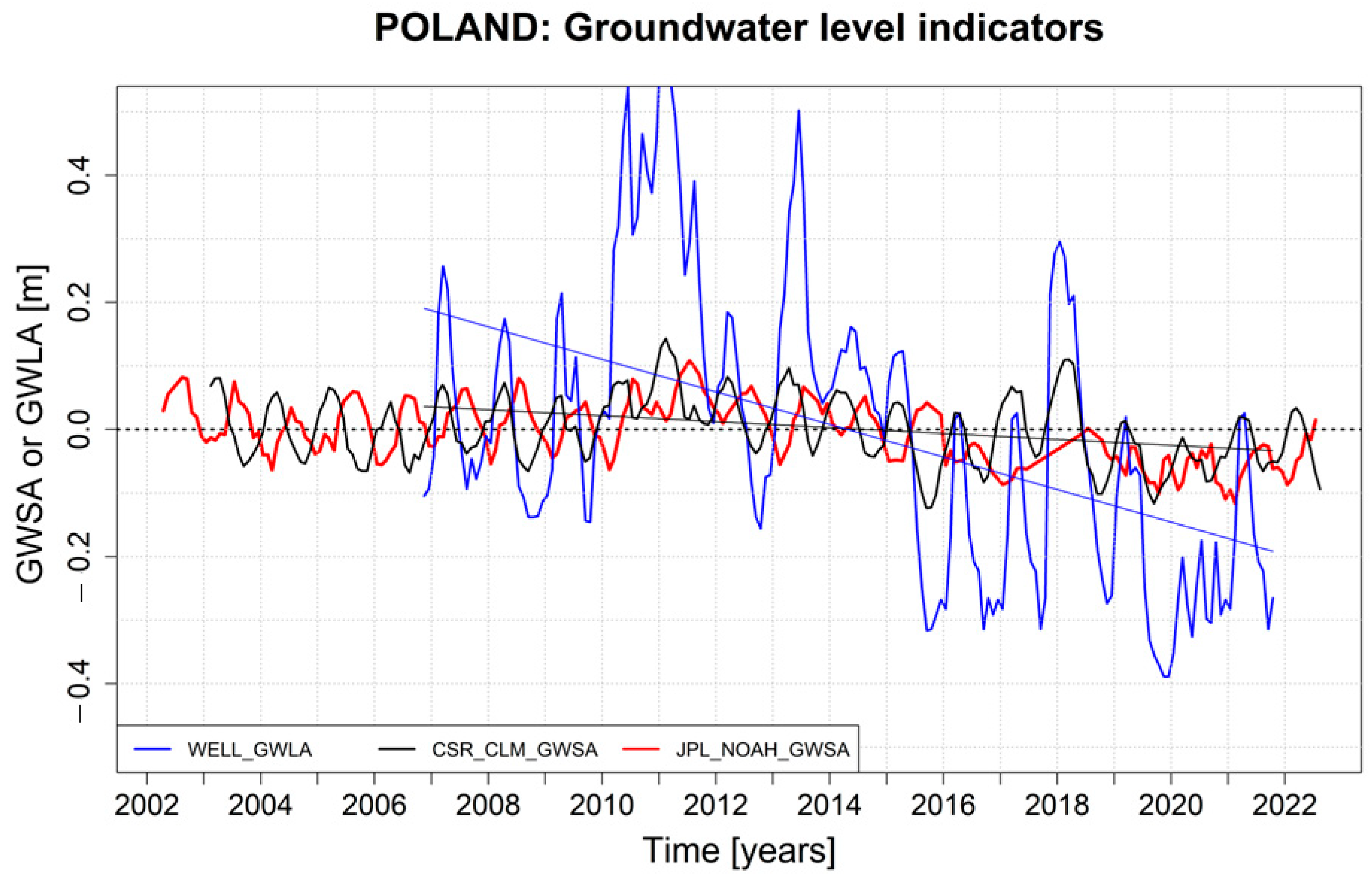
Figure 2 illustrates that the WELL_GWLA values generally exhibited a much greater range than the CSR_CLM_GWSA and JPL_NOAH_GWSA values. In particular, the observed seasonal peaks for Poland were, on average, four times greater than the model calculations in the considered period in the years 2003–2022. Similar results regarding this observation-to-model ratio were obtained in [7], showing a ratio of four. The ratio between groundwater storage change and groundwater level change is, from a hydrogeological viewpoint, known as the specific yield; see further interpretation and literature comparisons in the discussion section. In short, the specific yield is directly connected with the effective porosity (EP) of the ground in the vicinity of a well, expressing the total volume of open (spatially continuous) space that is not occupied by soil particles and is, hence, available for the groundwater. From the ratio of GWL to GWS, the volumetric effective porosity (% pore space per unit volume) can be estimated. In our case, GWLA, on average, is four times bigger than GWSA, which means that the (effective) porosity equals about 0.25. Minimum values of CSR_CLM_GWSA and wells were observed in autumn, which is related to high summer temperatures. However, maximum values were achieved in spring, which is generally related to snow melting after winter. In the case of JPL_NOAH_GWSA, the minimum values are reached in early spring, while the maximum values are reached in summer, i.e., a shift of about 1/4 of the year. The remote sensing results show a weak negative trend of about 5 mm/a (black regression line), whereas the observation well data show a more pronounced negative level trend of 40 mm/a (blue regression line). The trends were computed simultaneously with seasonal components.
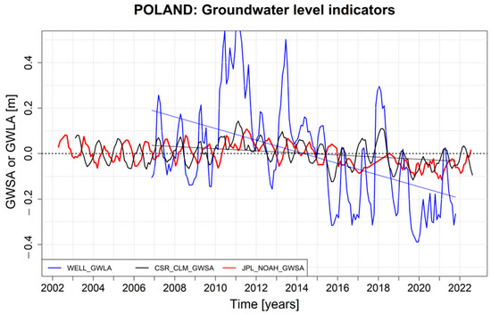
Figure 2.
Poland: Estimates of GWLA and GWSA, i.e., groundwater level anomalies (deviations) and groundwater storage anomalies relative to the mean groundwater level and storage (GWL and GWS) for the considered 2002–2022 period, as obtained from the time series of the observed WELL_GWLA (mean of 215 Polish wells, blue line), the derived CSR_CLM_GWSA (area average for Poland, black line) and the derived JPL_NOAH_GWSA (area average for Poland, red line). The thin, straight blue line shows the WELL_GWLA linear regression trend, and the thin, straight black line shows the CSR_CLM_GWSA linear regression trend.
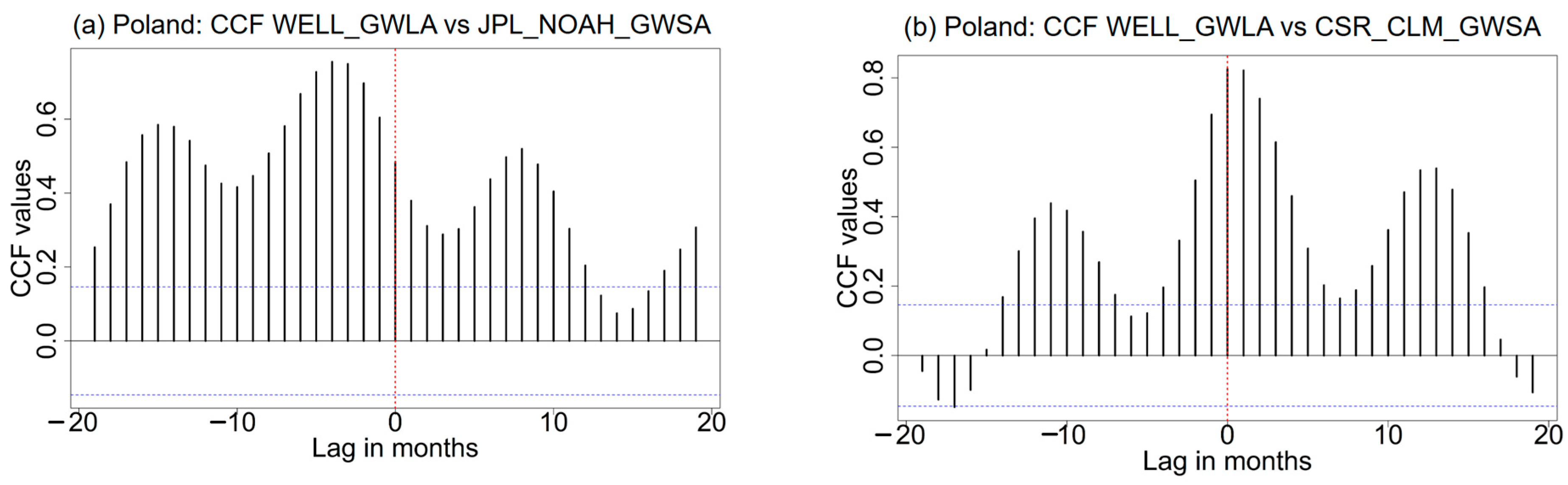
Figure 2 and the time cross-correlation functions (CCF) in Figure 3 show a strong correlation between CSR_CLM_GWSA and WELL_GWLA in Poland. The correlation coefficient at zero mutual shift of these two time series is approximately 0.8, indicating a high synchronization. However, Figure 2 and Figure 4 show evidence for a three-to-four-month shift between JPL_NOAH_GWSA and WELL_GWLA, suggesting a lack of synchronization between the GRACE—GLDAS NOAH data and the direct measurements. It seems that both positive and negative anomalies (i.e., peaks and valleys) in the in situ observations of groundwater levels in wells occur earlier than corresponding anomalies seen in the JPL_NOAH_GWSA model. This is despite the fact that [7] showed earlier that TWSA obtained from GRACE JPL alone, without subtracting the other water compartments from GLDAS NOAH data, are well synchronized with GWLA in wells in Poland (the correlation coefficient at lag = 0 was equal to 0.82). For GRACE JPL, it seems that subtracting water storage obtained from GLDAS NOAH to obtain the JPL_NOAH_GWSA results diminishes the correlation with wells for reasons that are further investigated below.
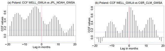
Figure 3.
Time cross-correlation functions CCF for (a) WELL_GWLA versus JPL_NOAH_GWSA, and (b) CCF for WELL_GWLA versus CSR_CLM_GWSA, considering the spatial average conditions of Poland.
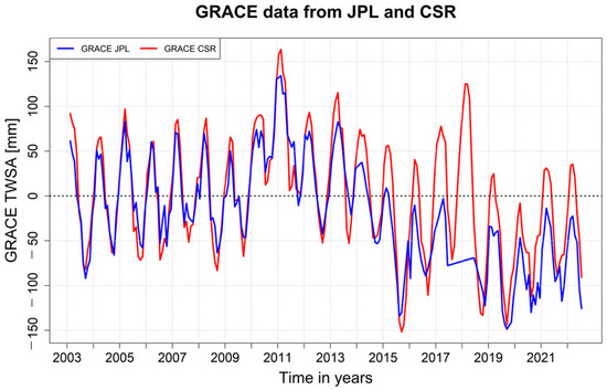
Figure 4.
GRACE TWSA obtained from JPL and CSR computational centres.
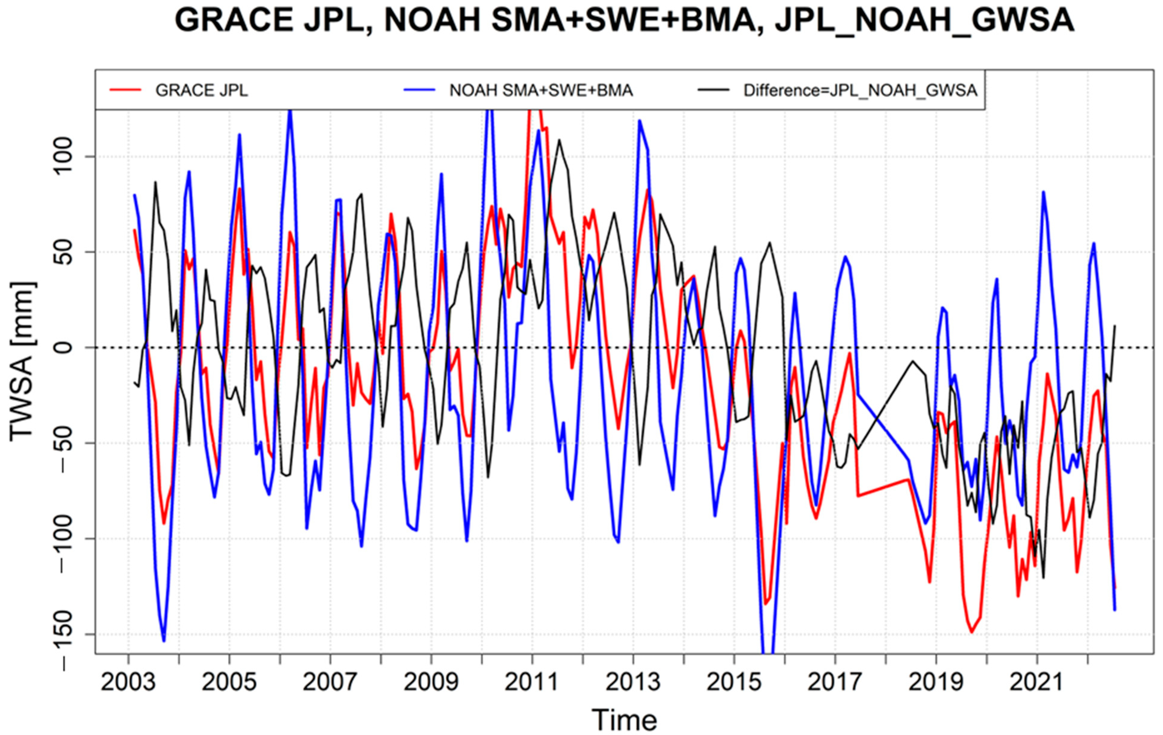
To understand the cause of the abovementioned inconsistencies, Figure 4 shows GRACE TWSA obtained from the JPL and CSR computing centres. Results show that the differences are relatively small, suggesting that the considerable inconsistencies between JPL_NOAH_GWSA and CSR_CLM_GWSA are not due to differences between the GRACE data from JPL and CSR. Considering the GRACE TWSA obtained from CSR, the SMA + SWEA + BMA obtained from the CLM model, and their differences that express the estimated values of CSR_CLM_GWSA (Figure 5), it is clear that the SMA + SWEA + BMA obtained from the CLM model are much smaller than the TWSA from GRACE. The differences between them, i.e., the estimated values of CSR_CLM_GWSA, have a smaller amplitude and unchanged phase when compared with the GRACE. Finally, Figure 6 shows GRACE TWSA obtained from JPL, SMA + SWEA + BMA obtained from the NOAH model, and their difference that shows estimated values of JPL_NOAH_GWSA. It can be seen that SMA + SWEA + BMA obtained from the NOAH model usually have a larger amplitude of changes than TWSA from GRACE (in contrast with the case of CLM in Figure 5), which causes a complete and erroneous reversal of the phase of the obtained JPL_NOAH_GWSA. For instance, as can be seen from Figure 5 and Figure 6, the ranges of NOAH SMA + SWEA + BMA changes in Poland are from −180 mm to +130 mm, while the corresponding ranges of CLM changes are from −40 mm to +40 mm, approximately. Similar patterns were also observed throughout Sweden. This confirms that changes in NOAH values are too large in the studied areas and do not match the results of direct measurements.
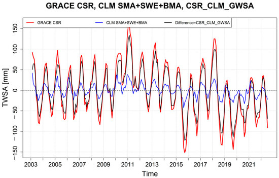
Figure 5.
CSR_CLM_GWSA obtained as the difference between CSR GRACE and CLM SMA + SWE + BMA.
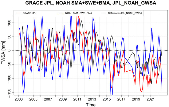
Figure 6.
JPL_NOAH_GWSA obtained as the difference between JPL GRACE and NOAH SMA + SWE + BMA.
5.2. Sweden
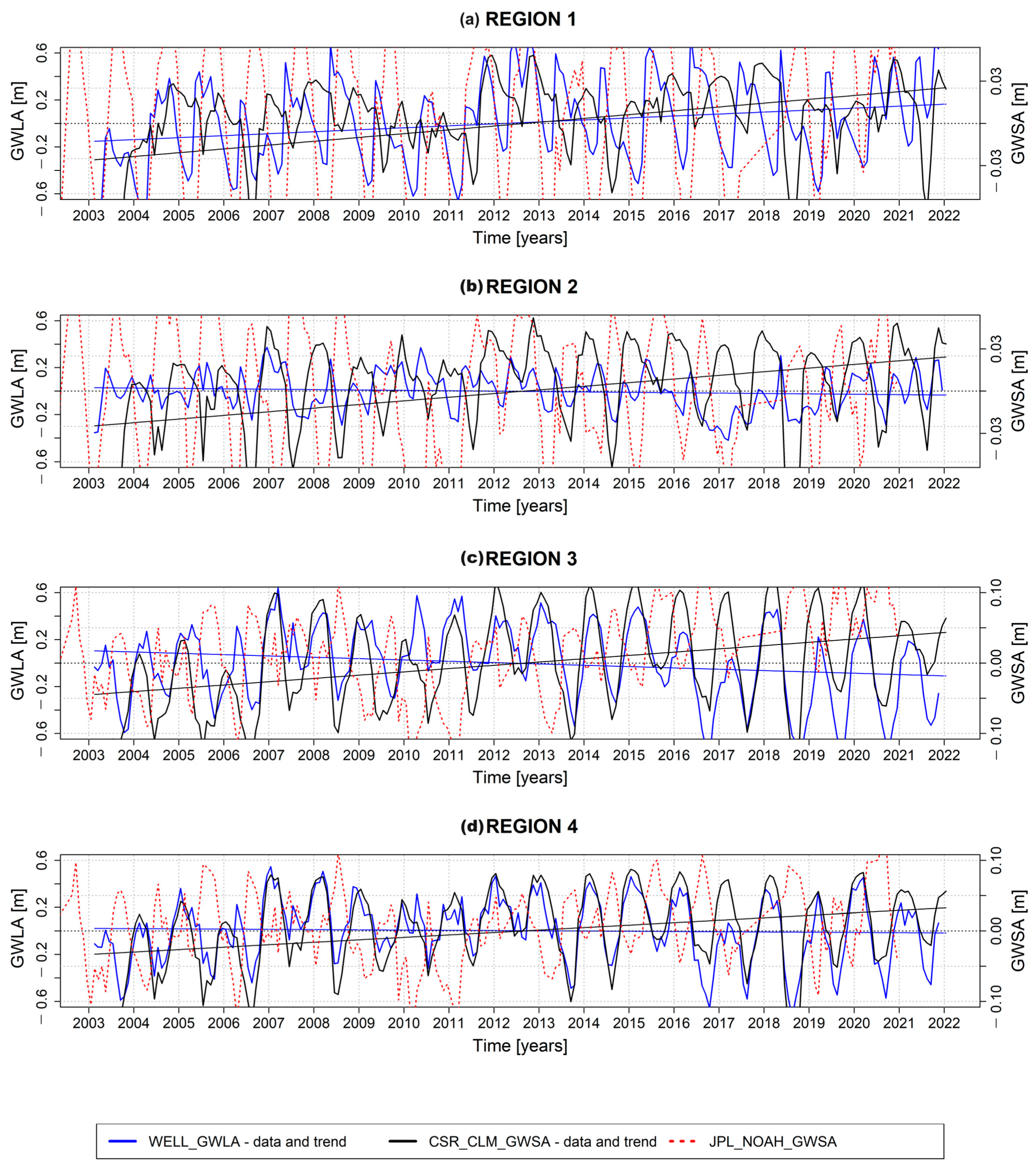
In Sweden, the WELL_GWLA value ranges are also generally much greater than the CSR_CLM_GWSA value ranges (see Figure 7 and note the differences in value range between the primary and secondary y-axis), as can also observed in Poland. The estimated approximate specific yield value for each region, which is equal to the effective porosity, was estimated by calculating the ratio between the differing GWSA and GWLA levels. We then obtained the values of 0.14 for region 1, 0.24 for region 2, and 0.17 for region 3 as well as for region 4 (in the case of JPL_NOAH_GWSA in comparison with WELL_GWSA), and the values of 0.08 for region 1, 0.21 for region 2 and region 3, and 0.22 for region 4 (in the case of CSR_CLM_GWSA in comparison with WELL_GWSA). Furthermore, annual minimum values of CSR_CLM_GWSA and WELL_GWLA most often occurred in autumn, particularly in the temperate regions 3 and 4 (Figure 7, blue and black curves, respectively), while the annual maximum values frequently occurred in spring, just as in Poland, which also has a temperate climate. However, the observed WELL_GWLA (blue curve) for the cold region 1 achieves maximum values in autumn and minimum in early spring (and additionally, WELL_GWLA for cold region 2 shows double peaks), none of which is captured by the remote sensing model (CSR_CLM_GWSA, black curve) that otherwise showed excellent performance in the temperate regions 3 and 4 (compare the blue and black curves). Regarding the long-term average groundwater storage in Sweden, the remote sensing results show increasing trends in all four regions, of between 3 and 5 mm/a (black regression lines), whereas the observation well data show diverging level trends from a decrease of ~10 mm/a in region 3 to an increase of ~14 mm/a in region 1 (blue regression lines).
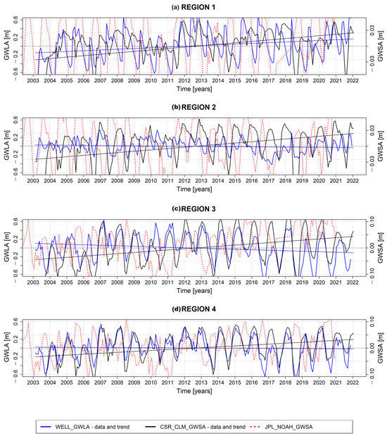
Figure 7.
Sweden: Estimates of the groundwater level anomalies (GWLA, i.e., deviations from period mean level) as obtained from the time series of WELL_GWLA, and groundwater storage anomalies (of model CSR_CLM_GWSA) for regions 1, 2, 3 and 4 ((a–d) respectively). The thin, straight blue and black lines show linear regression trends. The red dashed lines in the background show the course of GWSA determined from GRACE and NOAH.
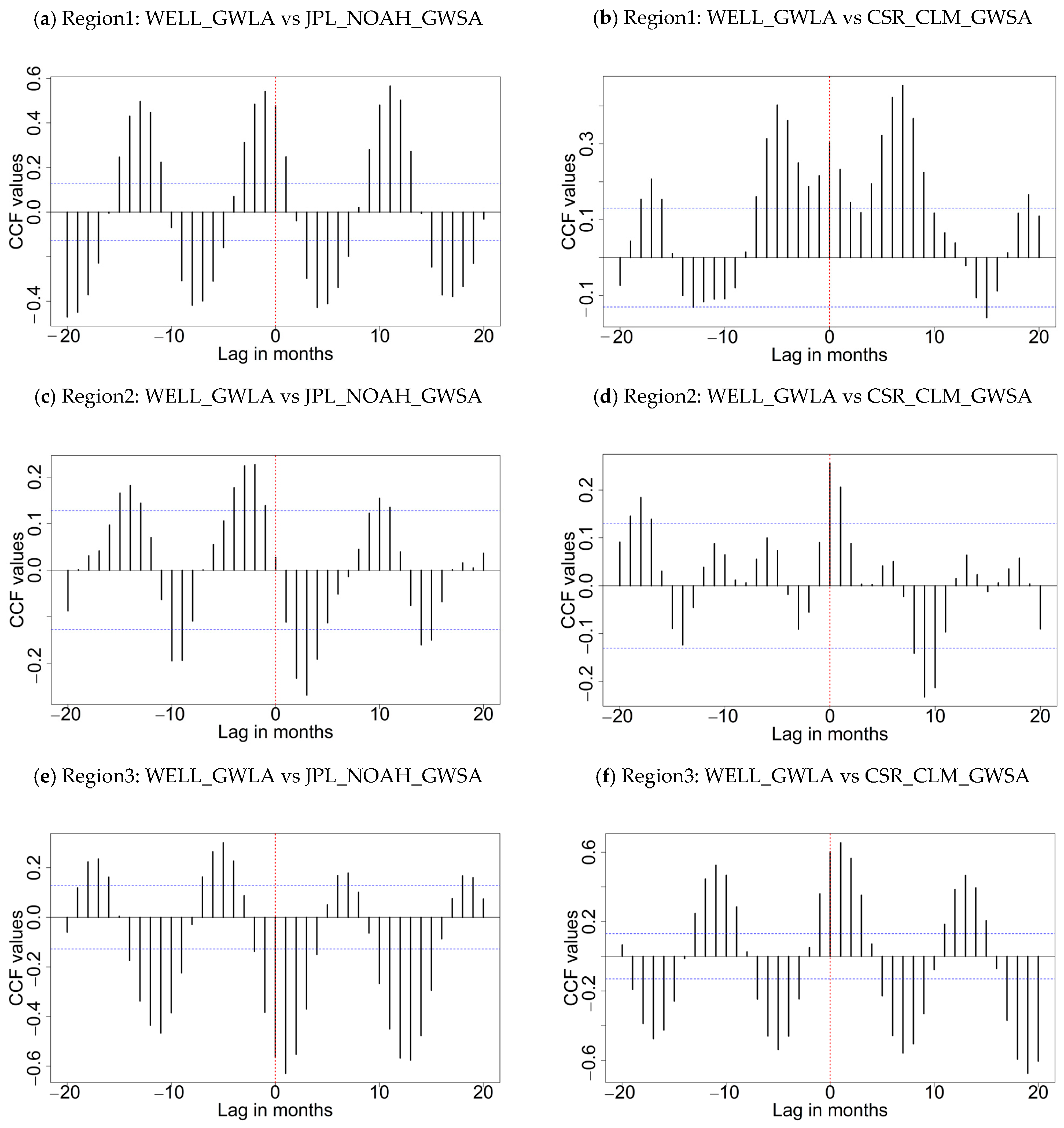
Overall, the match between CSR_CLM_GWSA and WELL_GWLA ranges from poor in northern Sweden to (very) good in southern Sweden (Figure 7). In region 1, the cross-correlation function (CCF) value between CSR_CLM_GWSA and WELL_GWLA for lag = 0 is approximately 0.3 (Figure 8b), much lower than in Poland. Its maximum values are for lag = 7 (0.45) and lag = −5 (−0.4) (Figure 8b). Additionally, the CCF was computed between WELL_GWLA and TWSA derived from JPL GRACE, showing a shift of 6 months (at lag = 0, the correlation is equal to −0.7, at lag = 6, it takes the value of about +0.6).
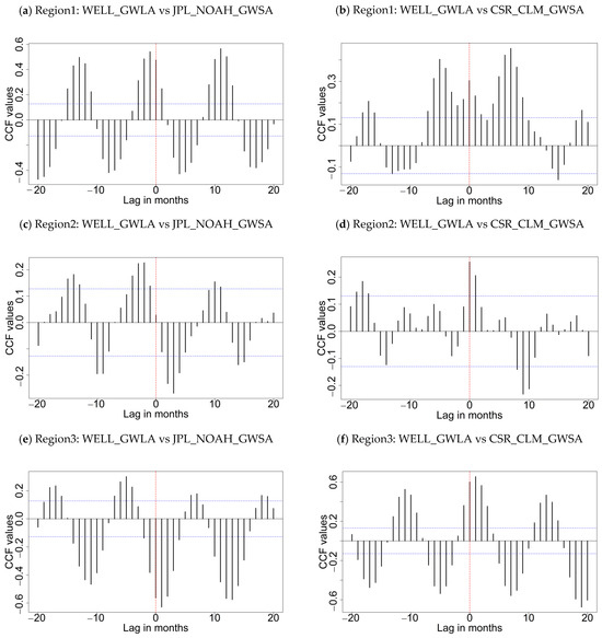
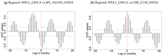
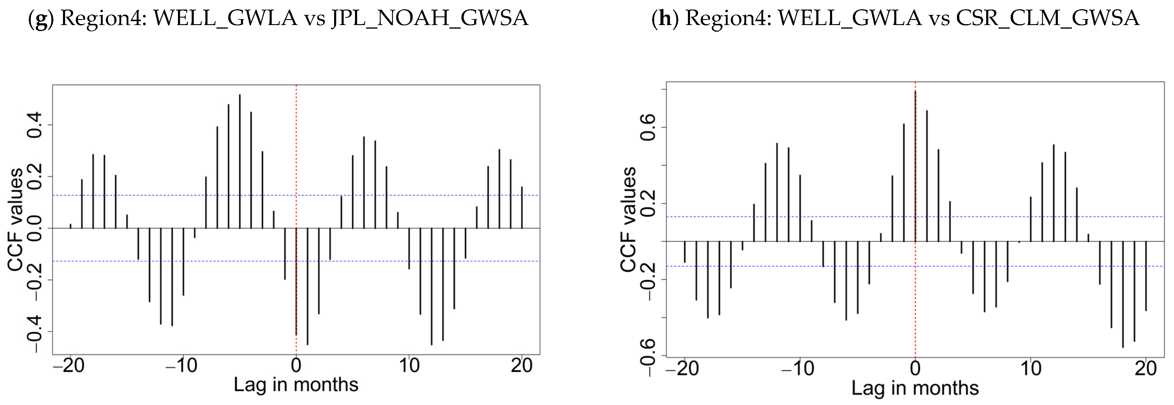
Figure 8.
Time cross-correlation functions CCF for WELL_GWLA versus JPL_NOAH_GWSA: (a,c,e,g) for regions 1, 2, 3, 4, respectively, and time cross-correlation functions CCF for WELL_GWLA versus CSR_CLM_GWSA (b,d,f,h).
In region 2, the values of the CCF are generally low, with the value of the correlation function between CSR_CLM_GWSA and WELL_GWLA for lag = 0 being approximately 0.26, which is also the maximum lag correlation within the investigated range (Figure 7b and Figure 8d). The largest negative correlation is at lag = 9 months and equals −0.23. Similarly, the CCF computed between WELL_GWLA and TWSA derived from JPL GRACE indicates generally weak correlations, such as a CCF value of about 0.3 at lag = 0, and a maximum value of 0.35.
In region 3, the values of the CCF are generally higher than those of region 2, ranging from −0.5 to 0.6 (Figure 8f). The value of the correlation function for lag = 0 is approximately 0.6, i.e., much higher than the Swedish regions 1 and 2 but slightly lower than in Poland. Its maximum occurs at lag = 1 (about 0.63, Figure 8f). The maximum negative correlation is at lag = 7 months, and it is equal to –0.55. The CCF was computed between the series of JPL_NOAH_GWSA and WELL_GWLA, showing a similar correlation between WELL_GWLA and CSR_CLM_GWSA, with the correlation of about 0.6 at lag = 0 (which is also the maximum of CCF).
In region 4, the values of the CCF are generally in the range of −0.5 to 0.8 (Figure 8h). The value of the correlation function for lag = 0 is approximately 0.77, and it is its maximum (Figure 8h), which is similarly good as that found for Poland. The biggest negative correlations occur at lag = 6, 18 months or lag = −6, −18, showing strong annual frequency present in the data. Additionally, the CCF was computed between GRACE JPL TWSA and WELL_GWLA. The results show that TWSA is also highly correlated with the wells fluctuations, with the correlation at lag = 0 amounting to about 0.72, which is the maximum of CCF in this case.
6. Discussion
The present analysis of the time cross-correlation function values between WELL_GWLA CSR_CLM_GWSA has shown a high degree of correlation (around 0.8) in Poland and southern Sweden (study regions 3 and 4). This is in contrast with the correlation values between WELL_GWLA and JPL_NOAH_GWSA, which never produced satisfactory results. The analysis has further shown that, in all of the considered regions, the NOAH values (sum of SMA, SWEA and BMA) showed changes that were too large and did not match the results of direct measurements, which largely explains the bad performance of JPL_NOAH_GWSA. This lack of match with measurements concerned not only the measured region average variation in WELL_GWLA, but also the local well measurements of the regions, implying that there were no smaller-scale exceptions to this model–measurement mismatch. This is illustrated for region 4 in Figure A2, Figure A3 and Figure A4 in Appendix A, showing that with few exceptions, the multi-annual peaks and low points for individual wells (grey lines) closely follow the region average variation (red line), all of which are distinctly different (shifted) compared with the pattern shown by the JPL_NOAH_GWSA model (Figure 7d). Taken together, it seems that GRACE data, coupled with the CLM model and the GRACE data alone, was not reduced by any model and best reflected the behaviour of the water level in the wells in most studied areas. GRACE’s total water storage data even offered a slightly better match with WELL GWLA.
The good fit (around 0.8) between the CSR_CLM_GWSA and observations (WELL_GWLA) in Poland (215 wells) and southern Sweden (172 wells) is consistent with other validation studies in temperate climate zones, e.g., a fit of 0.82 for the Algarve region in Portugal (having 51 wells [44]), 0.80 for Alberta in Canada (having 75 wells [31]), and 0.72 for karstic regions in SW China (having 17 wells [45]). In all of these regions, observation data show that they have groundwater regimes characterized by a clear (single peak) maximum level that occurs around the new year (January) in the Algarve region, in spring in Alberta, Poland and southern Sweden, and in summer in SW China. The generally high correlation coefficients reflect that the remote sensing models capture these seasonal patterns very well. In contrast, northern Sweden’s correlation coefficient was significantly lower (region 2). The present well data exhibits a pattern with double GWL peaks and double GWL low points (Figure 7b, blue line). These are caused by a lack of infiltration in winter months, which gives a low point in May (which is lacking in southern Sweden; SGU, RR). Then, following rising levels in (early) summer, there is another low point in fall caused by enhanced warm season evapotranspiration (seen in southern Sweden as a single low point). The remote sensing model does not reproduce these double peaks at all, despite the fact that its snow melt module tends to erroneously predict peaking GWL near the May low point, hence failing to capture the difference in groundwater regime between southern and northern Sweden (resulting in low correlation). Furthermore, in northernmost Sweden (region 1), summers are cool enough not to invoke the evapotranspiration-induced low point in fall (which is seen in the rest of Sweden). These further regime differences are not captured well (either) by the remote sensing model, as reflected in the low fit. The fact that the border of the good fit coincides with the relatively sharp border where the climate shifts from temperate to cold (sub-)Arctic [36,37], and the Swedish groundwater regime shifts accordingly from a more continental European behaviour to sub-Arctic and Arctic regimes [32], which are strongly governed by the cold-season blocking effect of ground frost on groundwater recharge. This suggests that the conventional methods for deriving GWSA cease to be reliable in the presence of considerably infiltration-blocking ground frost.
We note that the above-referred study showed a good fit between well observations and remote sensing model results in Alberta, which is similar to groundwater dynamics of northernmost Sweden (region 1), as obtained by [31], e.g., through condition adjustment (and downscaling). The corresponding fit for conventional data processing was 0.42, which is similar to the low results we obtained in northern Sweden; however, the authors of [32] did not consider hydrological process explanations for the differences in their presented results. More generally, the present process-based interpretation suggests that conventional remote sensing models cannot accurately represent groundwater level dynamics and seasonality under Arctic conditions (dominated by ground frost and/ or permafrost) unless the models are enhanced and validated. Unfortunately, complex environments such as the Arctic are recognized for their lack of validation data (e.g., [29]). Thus, leveraging data-rich (regional) patches from Swedish and Canadian monitoring networks may provide a constructive way forward in addressing regional processes, as well as generic (large-scale) open questions regarding the role of (moving) groundwater in Arctic energy budgets and associated permafrost melt and carbon releases (e.g., [45]).
Regarding long-term average trends in groundwater level, both well observations and remote sensing data suggest that average groundwater levels are decreasing in Poland (~10 mm/a), particularly over the last 10 years, which is consistent with previously reported results (e.g., [7]). Within Sweden, the observation well data (2003–2022) show weak but diverging trends, ranging from a decrease of ~10 mm/a in SE Sweden (region 3) to an increase of ~14 mm/a in northernmost Sweden (region 1), with regions 2 and 4 both having essentially no trend. Such decreasing GW level trends of SE Sweden, which contrast with maintained or increasing average GW levels in other parts of Sweden, have also been seen for earlier time periods (1980–2010), although possible hydroclimatic causes are not entirely clear [46]. However, the fact that SE Sweden has a decreasing trend in effective precipitation during unfrozen seasonal conditions, which is in contrast with other Swedish regions, suggests that the groundwater level trends reflect trends in effective precipitation [47]. In contrast with the observation data, the present remote sensing results indicated increasing trends for all four regions. In addition to possible errors related to the remote sensing method, groundwater pumping near observation wells has a potentially increasing impact. This is because they are often located near groundwater aquifers of interest for human water supply, whereas the remote sensing results will not be subject to such spatial biases. Such effects may be particularly pronounced during summer months (e.g., [48,49,50]), which is when the remote sensing results differed the most from the well observations in southern Sweden (region 3 and 4), where anthropogenic pressures from an increasing population are relatively high. The maintained increased groundwater storage in northern, sub-Arctic and Arctic Sweden is consistent with groundwater storage changes within the similar (positive) range reported from remote sensing studies for large Siberian rivers, including Ob, Yenisei and Lena. This positive trend is in contrast with decreasing groundwater storage reported for the large North American river basins of Mackenzie and Yukon [28,30].
In all of the examined cases, the amplitudes of WELL_GWLA changes were several times larger than those of JPL_NOAH_GWSA and CSR_CLM_GWSA changes. This effect was expected because water is constrained to the soil pore space (e.g., [7]). A low porosity will amplify water level changes due to a lack of available space for a given water volume change. Assuming negligible measurement errors and methodological errors, one can determine actual level changes across the landscape based on storage anomalies as ΔGWLA = ΔGWSA/EP where EP is the region average effective porosity (also denoted by the specific yield). Conversely, we have independently estimated both ΔGWLA and ΔGWSA in this study. As EP can additionally be reasonably constrained based on independently reported hydrogeological data, we have a basis upon which to discuss the extent to which the assumed equality holds true in the different regions, possibly identifying measurement-related or methodological causes for (any) deviations. Previous validation studies taking such an approach have shown that deviations from the assumed equality are frequently non-negligible, with errors up to 40% [51]. Such errors have mainly been attributed to uncertainties in the assumed representative (regional average) EP value under prevailing conditions of hydrogeological heterogeneity.
In the present study, the EP values for Poland approximated from the amplitudes of Figure 2 (ΔGWSA/ΔGWLA) were around 0.250, which is also reasonable from a hydrogeological perspective [7]. Similarly, for regions 2–4 in Sweden, EP derived from amplitudes of Figure 7b–d were around 0.20 (ranging from 0.17 to 0.24). A significant number of the associated observation wells were located in aquifers in coarse-grained glaciofluvial deposits containing gravel and sand (eskers), which have an estimated EP value of 0.15 (range 0.10–0.20; [52]). These two independent NE quantifications hence indicate that the relative absolute error is around 25%, which is well within the range of 40% mentioned in previous literature [52]. We note that the relatively high frequency of monitoring wells in and near eskers is due to the previously mentioned societal interest in groundwater storage changes in the large and deep groundwater aquifers used for water supply, which in turn is often related to the occurrence of eskers [32,53,54].
For northernmost Sweden (region 1), the EP derived from the amplitudes of Figure 5 were around 0.14. Although this is not far from the EP value for eskers of 0.15, there is a considerable difference in relative terms between the region 1 value of 0.14 and the region 2–4 values of 0.20. The lower values for region 1 could indicate generally different soil properties around the groundwater wells of that area. For example, around 20% of wells in region 1 are located in a limited area (see Figure 1) that is characterized by till soils (which are also common in other parts of Sweden [40]). Because till soils have a relatively low specific yield (approximately 0.05 [52]), their presence may have lowered the sample average. This also raises the more general question as to which extent the current density and distribution of groundwater wells in (northernmost) Sweden (~0.25 to 0.34 wells per 1000 km2) can approximately yield sample results that are representative of average level changes of the region. In the face of such observation data uncertainty, we cannot exclude that the average aquifer conditions are indeed different in northernmost Sweden, which may have implications for (future) GWSA data interpretations. Other potentially contributing factors to the low NE value of northernmost Sweden (when derived from amplitudes) include previously mentioned, non-negligible methodological errors related to the increased prevalence of ground frost and snow cover compared with the rest of the country and Poland. Within region 1, permafrost behaves similarly to solid rock, where water can only get through small cracks, resulting in relatively low EP values.
7. Conclusions
The aim of the paper was to assess the correlation of groundwater level changes obtained from direct measurements in wells with groundwater storage changes calculated using GRACE observation products and GLDAS models in Poland and Sweden. Monitoring groundwater is currently very important, as it is the most important source of water consumption. We attempted to enhance the understanding of differences in the accuracy of GWS change predictions obtained from the CSR GRACE and CLM GLDAS groundwater model and that from the JPL GRACE combined with NOAH GLDAS. Based on the research, we concluded the following:
- In temperate European climate zones (Poland and south Sweden), the CSR_CLM_GWSA model showed very good agreement with changes in 387 observation wells (cross-correlation coefficient of 0.8, implying a good performance of remote sensing models in representing seasonal groundwater dynamics, including amplitudes of groundwater level). However, the JPL_NOAH_GWSA model did not show satisfactory results as the NOAH values for key water balance terms (sum of SMA, SWEA and BMA) that were subtracted from TWSA to obtain GWSA were too large compared with direct measurements, which led to the over-correction of otherwise consistent TWSA results. The use of the JPL_NOAH_GWSA model should consequently be avoided, at least under temperate conditions similar to those investigated here.
- In sub-Arctic and Arctic climate zones, our comparison involving 85 wells in northern Sweden showed that the CSR_CLM_GWSA model results were poorly correlated with ground observations (cross-correlation coefficients of 0.3 or less).
This was found to be due to a general failure of the remote sensing model to reproduce the characteristic northern groundwater regime, which differed considerably from the characteristic regime shared by south Sweden and Poland. The failure was attributed to ground frost, which prevented (cold season) infiltration, leading to a trend of decreasing groundwater levels throughout the winter. The result emphasizes the need for model development in sub-Arctic and Arctic regions, including region-specific validation of commonly used remote sensing models.
The CSR_CLM_GWSA model should, therefore, not be used in cold region investigations, which is in contrast with its excellent performance when applied in temperate regions.
- Considering multi-annual (2003–2022) trends within the temperate climate regions, the remote sensing model indicated increasing groundwater levels in SW Sweden, whereas the region’s 59 wells indicated essentially unchanged conditions. For the 113 wells of SE Sweden, there was even disagreement on the direction of change. While the remote sensing model indicated increasing levels, the observations indicated a decreasing trend of ~10 mm/a. These discrepancies may, however, not necessarily be due to errors of the remote sensing model but may rather reflect impacts of anthropogenic pressures, which are higher near the observation wells that are often located in eskers used for water supply; consequently, this more generally emphasizes the potential significant roles of other pressures on water resources apart from climate change.
- For multi-annual groundwater trends of sub-Arctic and Arctic Sweden, the (more uncertain) remote sensing results nevertheless agree reasonably well with the groundwater well observations that show increasing groundwater levels of up to ~14 mm/a, which is consistent with reported trends of large Siberian river basins and in contrast with decreasing trends of large North American river basins.
Author Contributions
Conceptualization, Z.R. and M.B.; methodology, Z.R. and M.B.; software, Z.R..; validation, J.J., F.C. and J.P.; formal analysis, Z.R., M.B., J.J., F.C. and J.P.; investigation, Z.R., M.B., J.J., F.C. and J.P.; resources, Z.R., M.B., J.J., F.C. and J.P.; data curation, Z.R., M.B., J.J., F.C. and J.P.; writing—original draft preparation, Z.R., M.B., J.J., F.C. and J.P.; writing—review and editing, Z.R., M.B., J.J., F.C. and J.P.; visualization, Z.R.; supervision, Z.R. and J.J. All authors have read and agreed to the published version of the manuscript.
Funding
This research received no external funding.
Data Availability Statement
Data used in this paper can be acquired via the following links: well data in Poland: https://www.pgi.gov.pl/psh/materialy-informacyjne-psh/rocznik-hydrogeologiczny-psh.html, 20 January 2024; well data in Sweden: https://www.sgu.se/grundvatten/grundvattennivaer/matstationer/, 22 January 2023; CSR_CLM_GWS: https://hydro1.gesdisc.eosdis.nasa.gov/data/GLDAS/GLDAS_CLSM025_DA1_D.2.2/, 15 February 2024; JPL_GRACE: https://grace.jpl.nasa.gov/data/get-data/jpl_global_mascons/, 15 February 2024; NOAH products: https://podaac.jpl.nasa.gov/dataset/TELLUS_GLDAS-NOAH-3.3_TWS-ANOMALY_MONTHLY, 16 February 2023.
Conflicts of Interest
The authors declare no conflicts of interest.
Appendix A
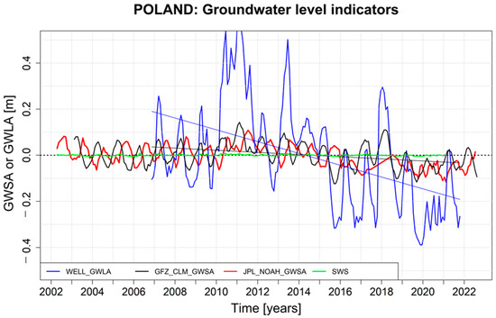
Figure A1.
Poland: Estimates of GWLA and GWSA, i.e., groundwater level anomalies (deviations) and groundwater storage anomalies relative to the mean groundwater level and storage (GWL and GWS) for the considered 2002–2022 period, as obtained from the time series of the observed WELL_GWLA (mean of 215 Polish wells, blue line), the derived CSR_CLM_GWSA (area average for Poland, green line) and the derived JPL_NOAH_GWSA (area average for Poland, red line).
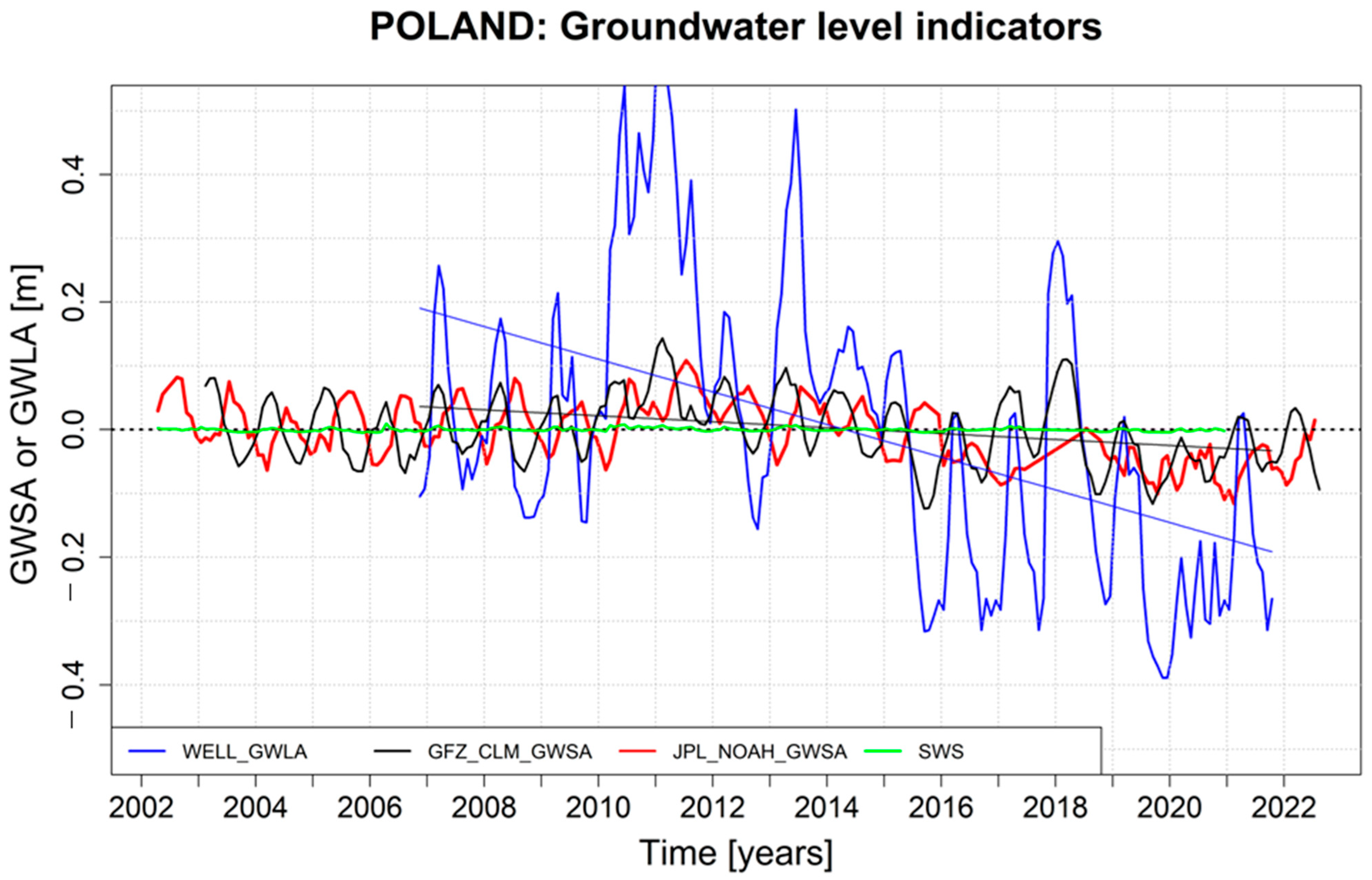
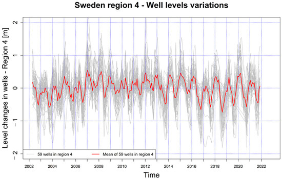
Figure A2.
Example from region 4 in Sweden, showing the multi-annual variations in groundwater level anomaly (WELL_GWLA) for each well of the region (grey lines), together with the region’s average variation in WELL_GWLA (red line, also displayed in Figure 7 as the blue line).
Figure A2.
Example from region 4 in Sweden, showing the multi-annual variations in groundwater level anomaly (WELL_GWLA) for each well of the region (grey lines), together with the region’s average variation in WELL_GWLA (red line, also displayed in Figure 7 as the blue line).

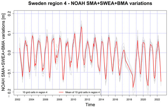
Figure A3.
Example from region 4 in Sweden, showing the multi-annual variations in NOAH data (SMA + SWEA + BMA) for each grid cell of the region (grey lines), together with the region’s average variation.
Figure A3.
Example from region 4 in Sweden, showing the multi-annual variations in NOAH data (SMA + SWEA + BMA) for each grid cell of the region (grey lines), together with the region’s average variation.
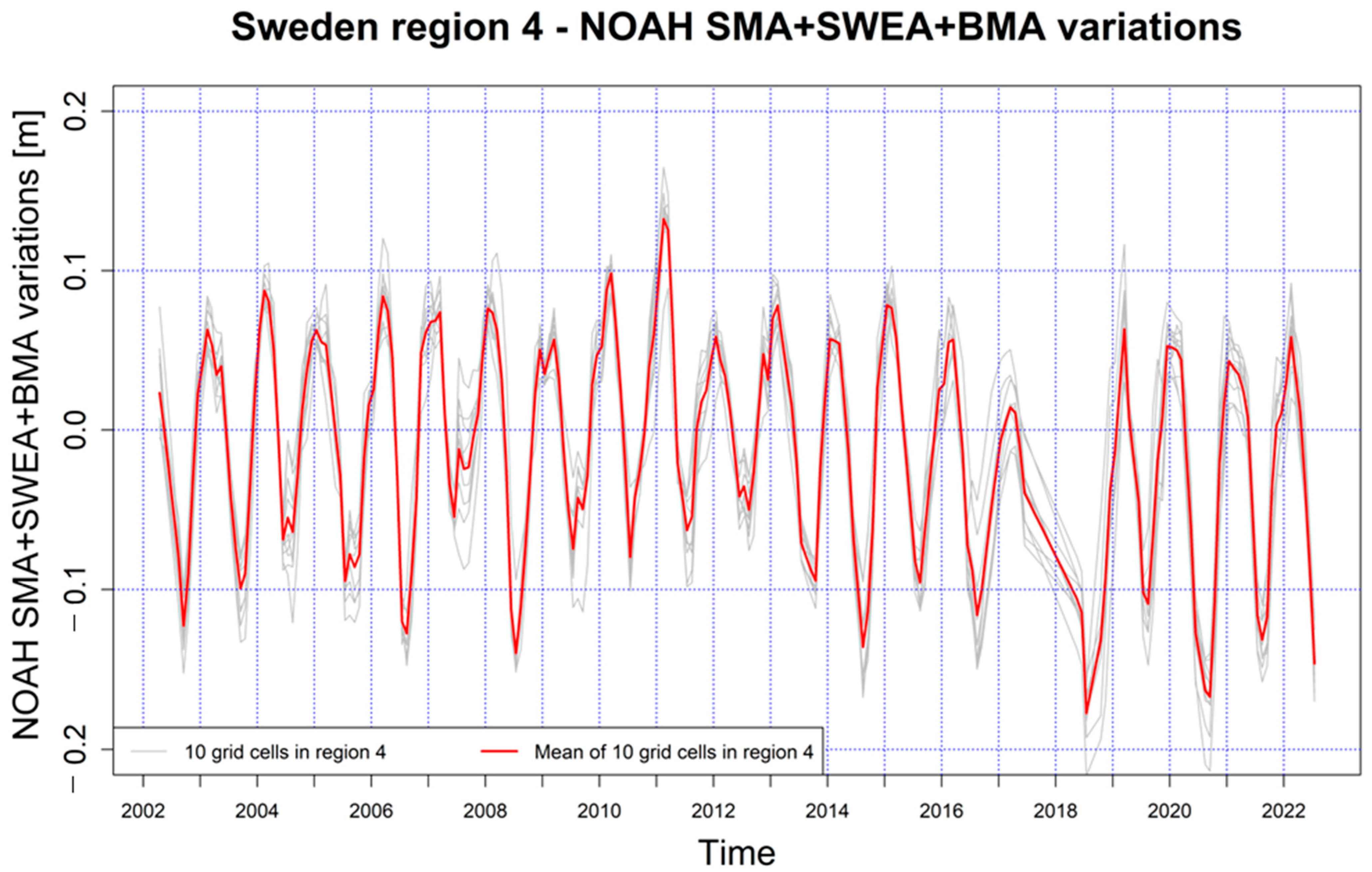
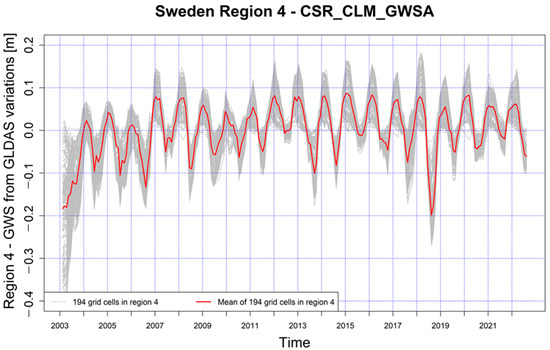
Figure A4.
Example from region 4 in Sweden, showing the multi-annual variations in CSR_CLM_GWSA for each cell of the region (grey lines), together with the region’s average variation (red line, also displayed in Figure 7 as the black line).
Figure A4.
Example from region 4 in Sweden, showing the multi-annual variations in CSR_CLM_GWSA for each cell of the region (grey lines), together with the region’s average variation (red line, also displayed in Figure 7 as the black line).
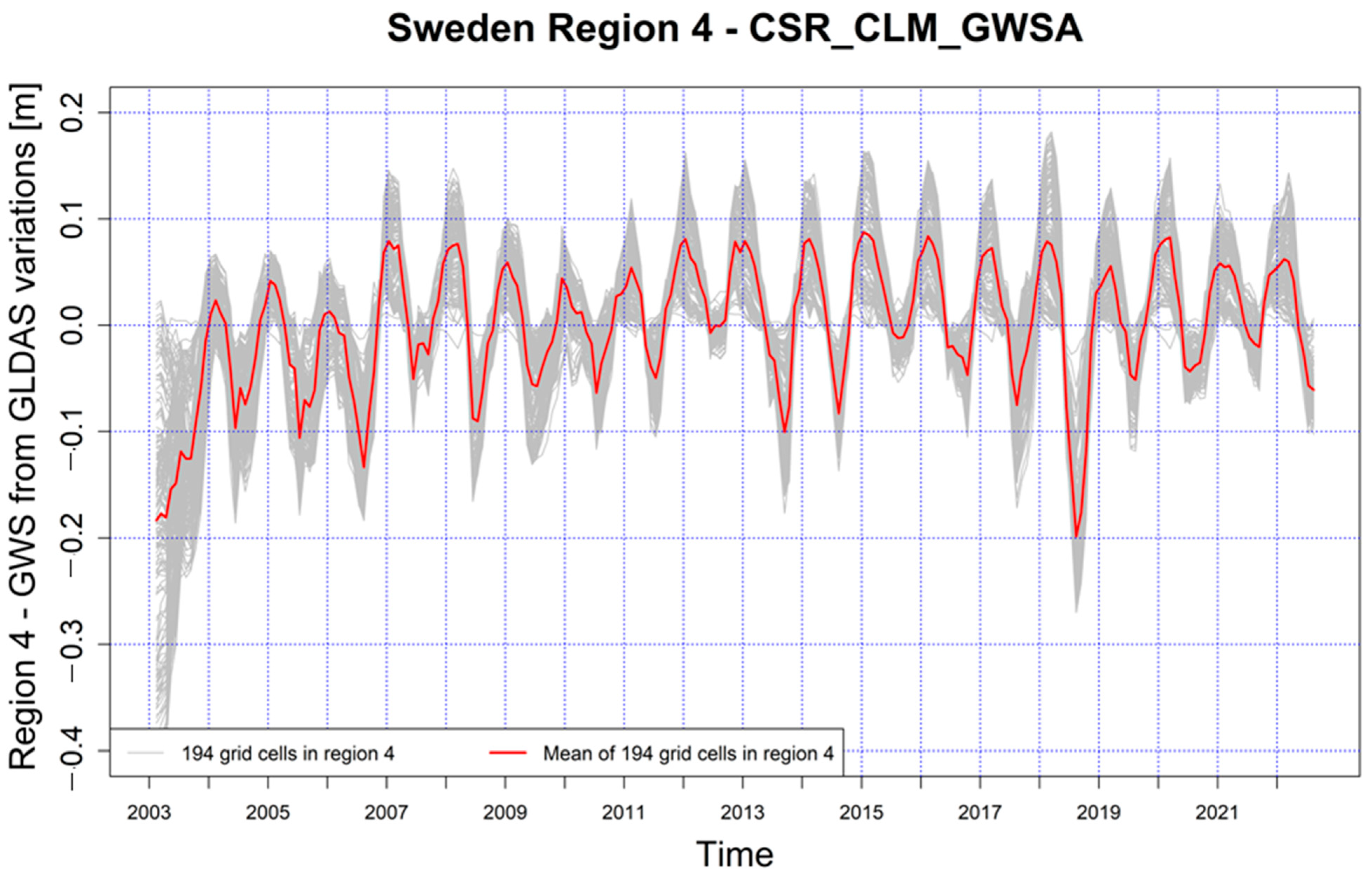
Figure A2, Figure A3 and Figure A4 show the average values used for the final calculations (red lines) compared with all of the components (individual measurement wells for Figure A2 and individual grid cells for Figure A3 and Figure A4) of these averages (grey lines). The examples shown refer to region 4 in Sweden. Averaging was performed for a different number of components, depending on the resolution of the input data.
References
- Guppy, L.; Uyttendaele, P.; Villholth, K.G.; Smakhtin, V. Groundwater and Sustainable Development Goals: Analysis of Inter-Linkages; United Nations University Institute for Water, Environment and Health: Hamilton, ON, Canada; ISBN 9789280860924.
- Solander, K.C.; Reager, J.T.; Wada, Y.; Famiglietti, J.S.; Middleton, R.S. GRACE satellite observations reveal the severity of recent water over-consumption in the United States. Sci. Rep. 2017, 7, 8723. [Google Scholar] [CrossRef]
- Tzanakakis, V.A.; Paranychianakis, N.V.; Angelakis, A.N. Water Supply and Water Scarcity. Water 2020, 12, 2347. [Google Scholar] [CrossRef]
- Śliwińska, J.; Birylo, M.; Rzepecka, Z.; Nastula, J. Analysis of Groundwater and Total Water Storage Changes in Poland Using GRACE Observations, In-situ Data, and Various Assimilation and Climate Models. Remote Sens. 2019, 11, 2949. [Google Scholar] [CrossRef]
- Landerer, F.W.; Flechtner, F.M.; Save, H.; Webb, F.H.; Bandikova, T.; Bertiger, W.I.; Bettadpur, S.V.; Byun, S.H.; Dahle, C.; Dobslaw, H.; et al. Extending the global mass change data record: Grace follow-on instrument and science data performance. Geophys. Res. Lett. 2020, 47, e2020GL088306. [Google Scholar] [CrossRef]
- Tapley, B.D.; Bettadpur, S.; Watkins, M.; Reigber, C. The gravity recovery and climate experiment: Mission overview and early results. Geophys. Res. Lett. 2004, 31, L09607. [Google Scholar] [CrossRef]
- Rzepecka, Z.; Birylo, M. Groundwater Storage Changes Derived from GRACE and GLDAS on Smaller River Basins—A Case Study in Poland. Geosciences 2020, 10, 124. [Google Scholar] [CrossRef]
- Karimi, H.; Iran-Pour, S.; Amiri-Simkooei, A.; Babadi, M. A gap-filling algorithm selection strategy for GRACE and GRACE Follow-On time series based on hydrological signal characteristics of the individual river basins. J. Géod. Sci. 2023, 13, 20220129. [Google Scholar] [CrossRef]
- Shao, C.; Liu, Y. Analysis of Groundwater Storage Changes and Influencing Factors in China Based on GRACE Data. Atmosphere 2023, 14, 250. [Google Scholar] [CrossRef]
- Pokhrel, Y.; Felfelani, F.; Satoh, Y.; Boulange, J.; Burek, P.; Gädeke, A.; Gerten, D.; Gosling, S.N.; Grillakis, M.; Gudmundsson, L.; et al. Global terrestrial water storage and drought severity under climate change. Nat. Clim. Chang. 2021, 11, 226–233. [Google Scholar] [CrossRef]
- Sinha, D.; Syed, T.H.; Famiglietti, J.S.; Reager, J.T.; Thomas, R.C. Characterizing drought in India using GRACE observations of terrestrial water storage deficit. J. Hydrometeorol. 2017, 18, 381–396. [Google Scholar] [CrossRef]
- Cooley, S.S.; Landerer, F.W. GRACE D-103133 Gravity Recovery and Climate Experiment Follow-On (GRACE-FO) Level-3 Data Product User Handbook; NASA Jet Propulsion Laboratory, California Institute of Technology: Pasadena, CA, USA, 2019.
- Li, M.; Wu, P.; Ma, Z.; Lv, M.; Yang, Q.; Duan, Y. The decline in the groundwater table depth over the past four decades in China simulated by the Noah-MP land model. J. Hydrol. 2022, 607, 127551. [Google Scholar] [CrossRef]
- Birylo, M.; Rzepecka, Z.; Nastula, J. Assessment of the Water Budget from GLDAS Model. In Proceedings of the 2018 Baltic Geodetic Congress (BGC Geomatics), Olsztyn, Poland, 21–23 June 2018. [Google Scholar] [CrossRef]
- Verma, K.; Katpatal, Y.B. Groundwater Monitoring Using GRACE and GLDAS Data after Downscaling within Basaltic Aquifer System. Groundwater 2018, 58, 143–151. [Google Scholar] [CrossRef]
- Schumacher, M.; Forootan, E.; van Dijk, A.I.J.M.; Schmied, H.M.; Crosbie, R.S.; Kusche, J.; Doell, P. Improving drought simulations within the Murray-Darling Basin by combined calibration/assimilation of GRACE data into the WaterGAP Global Hydrology Model. Remote Sens. Environ. 2018, 204, 212–228. [Google Scholar] [CrossRef]
- Rodell, M.; Chen, J.; Kato, H.; Famiglietti, J.S.; Nigro, J.; Wilson, C.R. Estimating groundwater storage changes in the Mississippi River basin (USA) using GRACE. Hydrogeol. J. 2006, 15, 159–166. [Google Scholar] [CrossRef]
- Badora, D. Studium wykorzystania modelu GRACE w ocenie zmian poziomu wód gruntowych w kontekście dostępności wody dla rolnictwa w zlewni rzeki Wisły. Pol. J. Agron. 2016, 27, 21–31. [Google Scholar] [CrossRef]
- Badora, D.; Wawer, R. Review of selected geophysical methods used in the assessment of water resources for agriculture. Pol. J. Agron. 2018, 34, 23–33. [Google Scholar] [CrossRef]
- Lenczuk, A.; Klos, A.; Bogusz, J. Studying spatio-temporal patterns of vertical displacements caused by groundwater mass changes observed with GPS. Remote Sens. Environ. 2023, 292, 113597. [Google Scholar] [CrossRef]
- Taylor, C.J.; Alley, W.M. Ground-Water-Level Monitoring and the Importance of Long-Term Water-Level Data; US Geological Survey: Denver, CO, USA, 2001; Volume 1217.
- Megdal, S.B.; Gerlak, A.K.; Varady, R.G.; Huang, L. Groundwater governance in the United States: Common priorities and challenges. Groundwater 2015, 53, 677–684. [Google Scholar] [CrossRef] [PubMed]
- Araújo, R.S.; da Gloria Alves, M.; de Melo, M.T.C.; Chrispim, Z.M.; Mendes, M.P.; Júnior, G.C.S. Water resource management: A comparative evaluation of Brazil, Rio de Janeiro, the European Union, and Portugal. Sci. Total Environ. 2015, 511, 815–828. [Google Scholar] [CrossRef]
- Chinnasamy, P.; Maheshwari, B.; Prathapar, S. Understanding Groundwater Storage Changes and Recharge in Rajasthan, India through Remote Sensing. Water 2015, 7, 5547–5565. [Google Scholar] [CrossRef]
- Inoue, J.; Yamazaki, A.; Ono, J.; Dethloff, K.; Maturilli, M.; Neuber, R.; Edwards, P.; Yamaguchi, H. Additional Arctic observations improve weather and sea-ice forecasts for the Northern Sea Route. Sci. Rep. 2015, 5, 16868. [Google Scholar] [CrossRef] [PubMed]
- Duncan, B.N.; Ott, L.E.; Abshire, J.B.; Brucker, L.; Carroll, M.L.; Carton, J.; Comiso, J.C.; Dinnat, E.P.; Forbes, B.C.; Gonsamo, A.; et al. Space-Based Observations for Understanding Changes in the Arctic-Boreal Zone. Rev. Geophys. 2009, 8, e2019RG000652. [Google Scholar] [CrossRef]
- Müller, F.L.; Dettmering, D.; Bosch, W.; Seitz, F. Monitoring the Arctic Seas: How Satellite Altimetry Can Be Used to Detect Open Water in Sea-Ice Regions. Remote Sens. 2017, 9, 551. [Google Scholar] [CrossRef]
- Muskett, R.R.; Romanovsky, V.E. Groundwater storage changes in arctic permafrost watersheds from GRACE and in situ measurements. Environ. Res. Lett. 2009, 4, 045009. [Google Scholar] [CrossRef]
- Frappart, F.; Papa, F.; Güntner, A.; Werth, S.; Ramillien, G.; Prigent, C.; Bonnet, M.P. Interannual variations of the terrestrial water storage in the Lower Ob’Basin from a multisatellite approach. Hydrol. Earth Syst. Sci. 2010, 14, 2443–2453. [Google Scholar] [CrossRef]
- Zuo, J.; Xu, J.; Chen, Y.; Li, W. Downscaling simulation of groundwater storage in the Tarim River basin in northwest China based on GRACE data. Phys. Chem. Earth 2021, 123, 103042. [Google Scholar] [CrossRef]
- Eveborn, D.; Vikberg, E.; Thunholm, B.; Hjerne, C.E.; Gustafsson, M. Grundvattenbildning och Grundvattentillgång i Sverige; Geological Survey of Sweden: Uppsala, Sweden, 2017. [Google Scholar]
- Krogulec, E.; Zabłocki, S.; Sawicka, K. Changes in groundwater regime during vegetation period in Groundwater Dependent Ecosystems. Acta Geol. Pol. 2016, 66, 525–540. [Google Scholar] [CrossRef]
- Rzepecka, Z.; Birylo, M.; Kuczynska-Siehien, J. Analysis of groundwater level variations and water balance in the area of the Sudety mountains. Acta Geodyn. Geomater. 2017, 14, 313–321. [Google Scholar] [CrossRef]
- Ehlert, K. Avrinningsområden i Sverige. Del 1. Vattendrag till Bottenviken: Svenskt Vattenarkiv 2020. Available online: https://www.smhi.se/polopoly_fs/1.164669!/Hydrologi_82%20Avrinningsomr%C3%A5den%20i%20Sverige.%20Del%201.%20Vattendrag%20till%20Bottenviken.pdf (accessed on 10 May 2023).
- Save, H.; Bettadpur, S.; Tapley, B.D. High-resolution CSR GRACE RL05 mascons. J. Geophys. Res. Solid Earth 2016, 121, 7547–7569. [Google Scholar] [CrossRef]
- Kottek, M.; Grieser, J.; Beck, C.; Rudolf, B.; Rubel, F. World map of the Köppen-Geiger climate classification updated. Meteorol. Z. 2006, 15, 259–263. [Google Scholar] [CrossRef]
- Chen, D.; Chen, H.W. Using the Köppen classification to quantify climate variation and change: An example for 1901–2010. Environ. Dev. 2013, 6, 69–79. [Google Scholar] [CrossRef]
- Watkins, M.M.; Wiese, D.N.; Yuan, D.-N.; Boening, C.; Landerer, F.W. Improved methods for observing Earth’s time variable mass distribution with GRACE using spherical cap mascons. J. Geophys. Res. Solid Earth 2015, 120, 2648–2671. [Google Scholar] [CrossRef]
- Wiese, D.N.; Landerer, F.W.; Watkins, M.M. Quantifying and reducing leakage errors in the JPL RL05M GRACE mascon solution. Water Resour. Res. 2016, 52, 7490–7502. [Google Scholar] [CrossRef]
- Li, B.; Rodell, M.; Sheffield, J.; Wood, E.; Sutanudjaja, E. Long-term, non-anthropogenic groundwater storage changes simulated by three global-scale hydrological models. Sci. Rep. 2019, 9, 10746. [Google Scholar] [CrossRef]
- Ali, S.; Liu, D.; Fu, Q.; Cheema, M.J.M.; Pham, Q.B.; Rahaman, M.M.; Dang, T.D.; Anh, D.T. Improving the Resolution of GRACE Data for Spatio-Temporal Groundwater Storage Assessment. Remote Sens. 2021, 13, 3513. [Google Scholar] [CrossRef]
- Neves, M.C.; Nunes, L.M.; Monteiro, J.P. Evaluation of GRACE data for water resource management in Iberia: A case study of groundwater storage monitoring in the Algarve region. J. Hydrol. Reg. Stud. 2020, 32, 100734. [Google Scholar] [CrossRef]
- Shumway, R.H.; Stoffer, D.S. Time Series Analysis and Its Applications, 4th ed.; Springer: Berlin/Heidelberg, Germany, 2016. [Google Scholar]
- Huang, F.; Zhang, Y.; Zhang, D.; Chen, X. Environmental Groundwater Depth for Groundwater-Dependent Terrestrial Ecosystems in Arid/Semiarid Regions: A Review. Int. J. Environ. Res. Public Health 2019, 16, 763. [Google Scholar] [CrossRef]
- Hamm, A.; Frampton, A. Impact of lateral groundwater flow on hydrothermal conditions of the active layer in a high-Arctic hillslope setting. Cryosphere 2021, 15, 4853–4871. [Google Scholar] [CrossRef]
- Nygren, M.; Giese, M.; Barthel, R. Recent trends in hydroclimate and groundwater levels in a region with seasonal frost cover. J. Hydrol. 2021, 602, 126732. [Google Scholar] [CrossRef]
- Hachborn, E.; Berg, A.; Levison, J.; Ambadan, J.T. Sensitivity of GRACE-derived estimates of groundwater-level changes in southern Ontario, Canada. Hydrogeol. J. 2017, 25, 2391–2402. [Google Scholar] [CrossRef]
- Rateb, A.; Scanlon, B.R.; Pool, D.R.; Sun, A.; Zhang, Z.; Chen, J.; Clark, B.; Faunt, C.C.; Haugh, C.J.; Hill, M.; et al. Comparison of Groundwater Storage Changes from GRACE Satellites with Monitoring and Modeling of Major U.S. Aquifers. Water Resour. Res. 2020, 56, e2020WR027556. [Google Scholar] [CrossRef]
- Strassberg, G.; Scanlon, B.R.; Rodell, M. Comparison of Seasonal Terrestrial Water Storage Variations from GRACE with Groundwater-Level Measurements from the High Plains Aquifer (USA). Geophys. Res. Lett. 2007, 34. [Google Scholar] [CrossRef]
- Birylo, M.; Rzepecka, Z. Remote Sensing-Based Hydro-Extremes Assessment Techniques for Small Area Case Study (The Case Study of Poland). Remote Sens. 2023, 15, 5226. [Google Scholar] [CrossRef]
- Rodhe, A.; Lindström, G.; Dahné, J. Grundvattennivåer i Ett Förändrat Klimat; Slutrapport Från SGU-Projektet; Grundvattenbildning i Ett Förändrat Klimat; SGUs Diarienummer 60-1642; Institutionen för Geovetenskaper, Uppsala Universitet: Uppsala, Sweden, 2007. [Google Scholar]
- Nadeau, S.; Rosa, E.; Cloutier, V.; Daigneault, R.-A.; Veillette, J. A GIS-based approach for supporting groundwater protection in eskers: Application to sand and gravel extraction activities in Abitibi-Témiscamingue, Quebec, Canada. J. Hydrol. Reg. Stud. 2015, 4, 535–549. [Google Scholar] [CrossRef]
- Barthel, R.; Stangefelt, M.; Giese, M.; Nygren, M.; Seftigen, K.; Chen, D. Current understanding of groundwater recharge and groundwater drought in Sweden compared to countries with similar geology and climate. Geogr. Ann. Ser. A Phys. Geogr. 2021, 103, 323–345. [Google Scholar] [CrossRef]
- Sparrenbom, C.; Jeppsson, H.; Appelo, T.; Barmen, G.; Barth, J.; Dahlin, T.; Dahlqvist, P.; Dopson, M.; O Ericsson, L.; Fagerlund, F.; et al. Grundvattenboken; Studentlitteratur AB: Lund, Sweden, 2022. [Google Scholar]


Disclaimer/Publisher’s Note: The statements, opinions and data contained in all publications are solely those of the individual author(s) and contributor(s) and not of MDPI and/or the editor(s). MDPI and/or the editor(s) disclaim responsibility for any injury to people or property resulting from any ideas, methods, instructions or products referred to in the content. |
© 2024 by the authors. Licensee MDPI, Basel, Switzerland. This article is an open access article distributed under the terms and conditions of the Creative Commons Attribution (CC BY) license (https://creativecommons.org/licenses/by/4.0/).