

Monsoon-Based Linear Regression Analysis for Filling Data Gaps in Gravity Recovery and Climate Experiment Satellite Observations


Abstract
1. Introduction
- Utilizing other satellite data.
- 2.
- Artificial Intelligence, Machine Learning, and Deep Learning.
- 3.
- Mathematical and Statistical Methods.
2. Materials and Methods
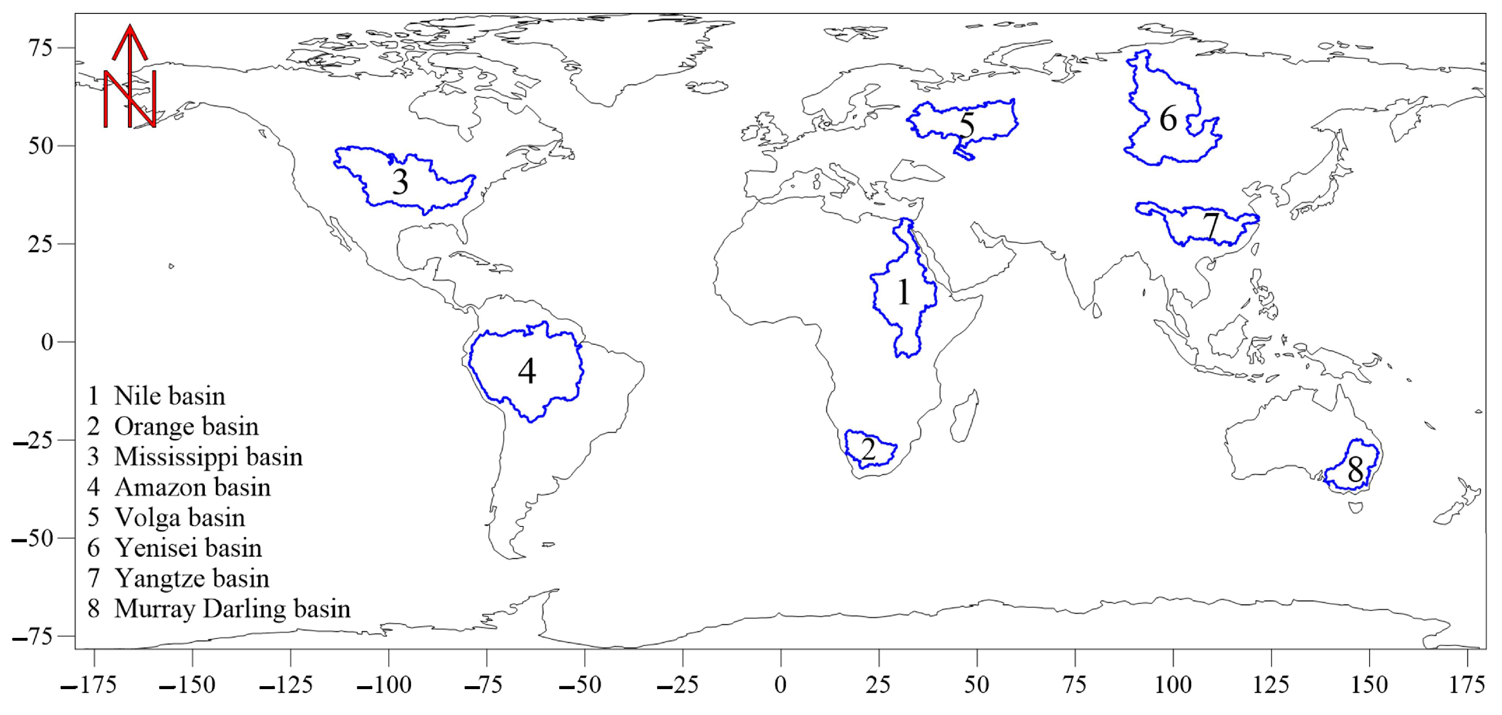
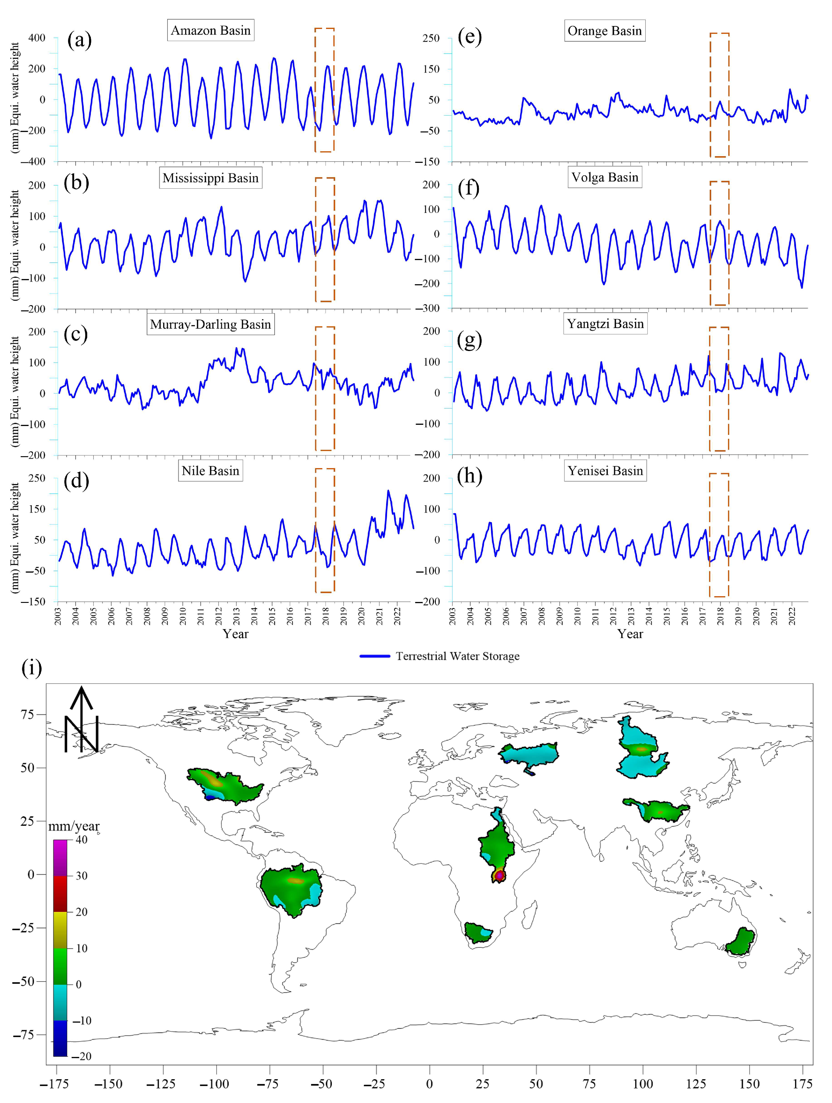
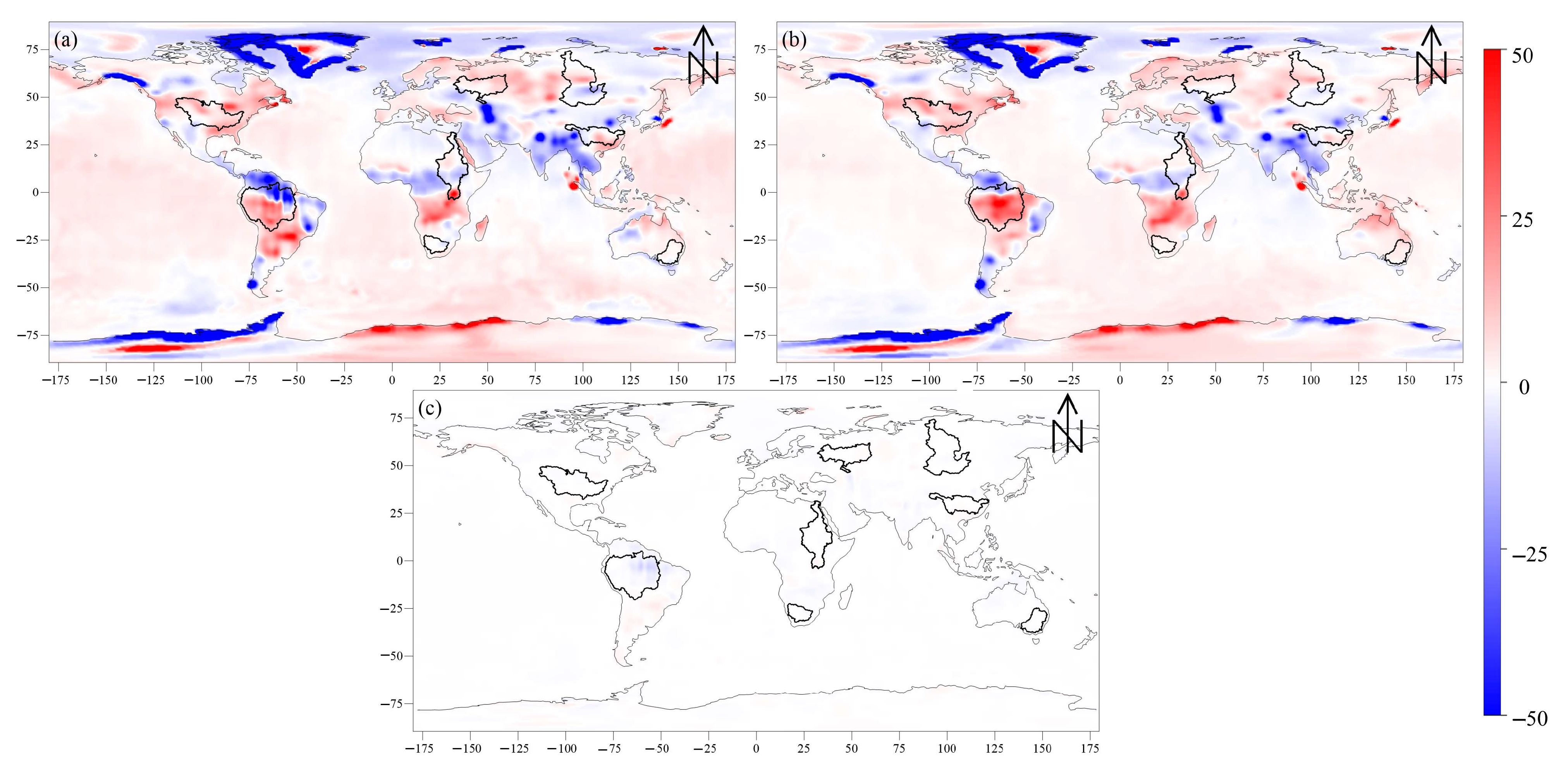
2.1. Study Area
2.2. Gravity Data
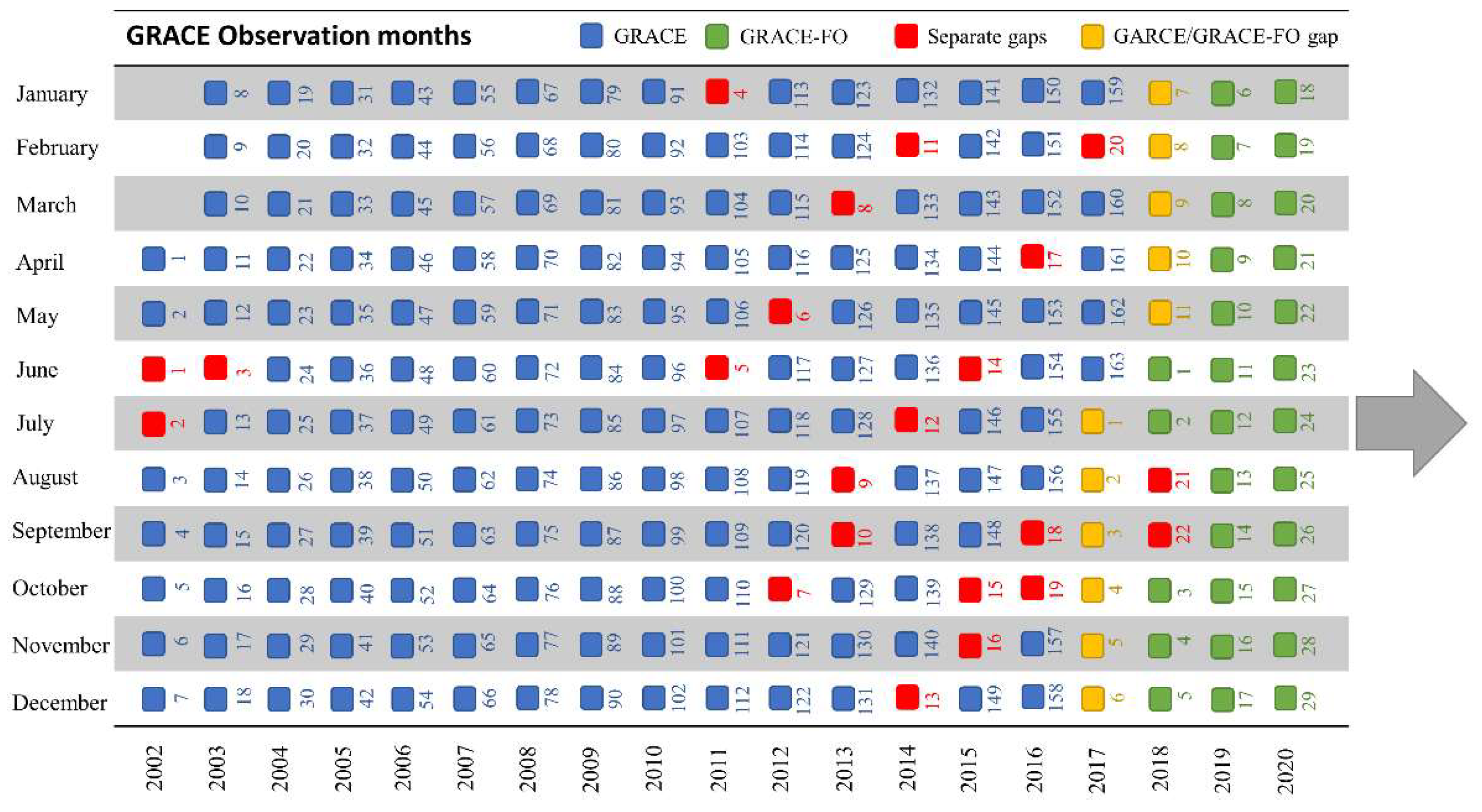
2.2.1. GRACE Data
2.2.2. Swarm Data
2.2.3. IGG
2.2.4. Quantum Frontiers (QFs)
2.2.5. Singular Spectrum Analysis (SSA) Coefficients
2.3. Monsoon Linear Regression Analysis (LRA) Method
2.4. Gap-Filling Model Using LRA
3. Comparison between LRA Model and Other Filling-In Models
4. Results and Discussion
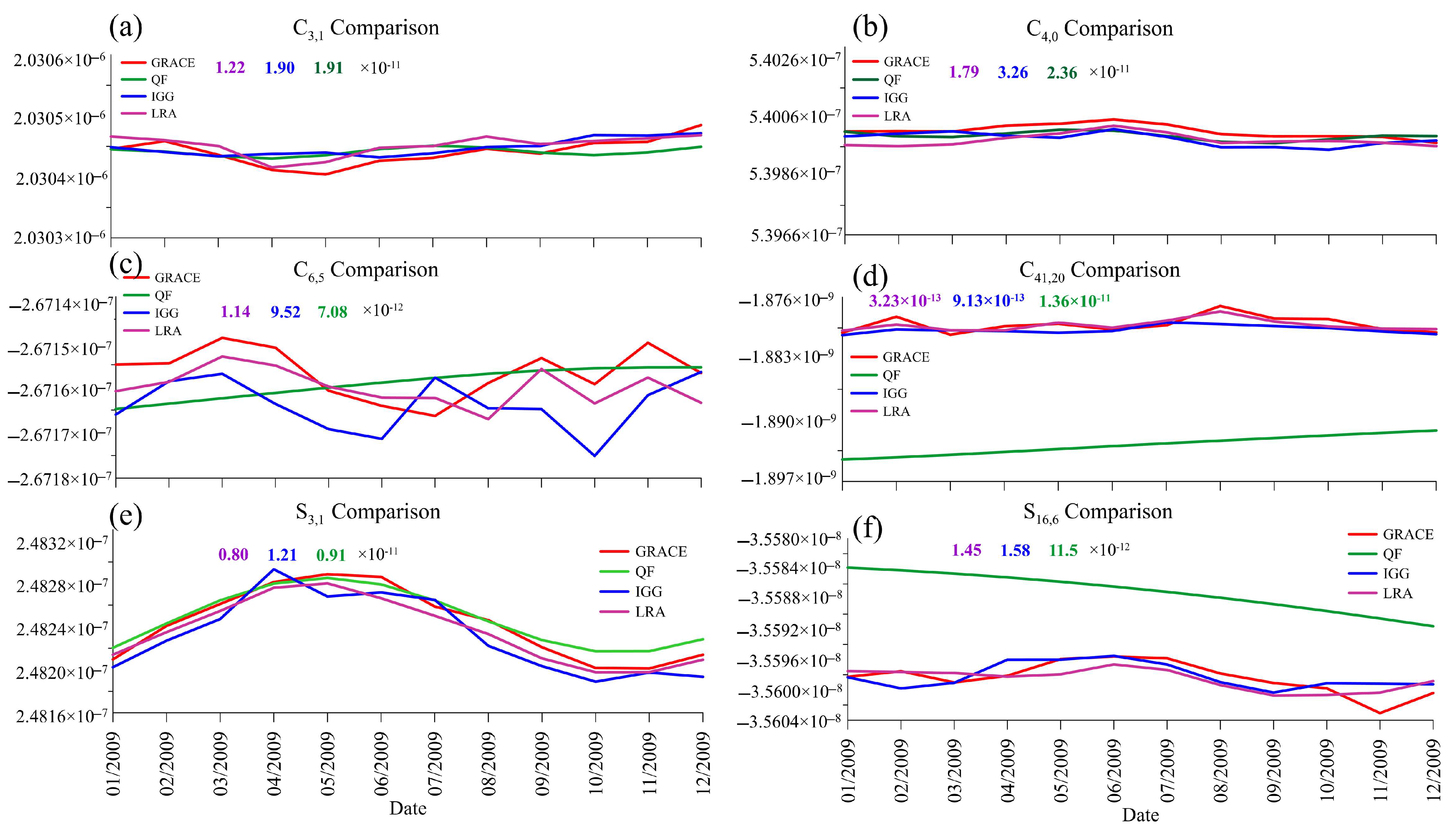
4.1. Spectral Domain: Artificial Gap in GRACE Era
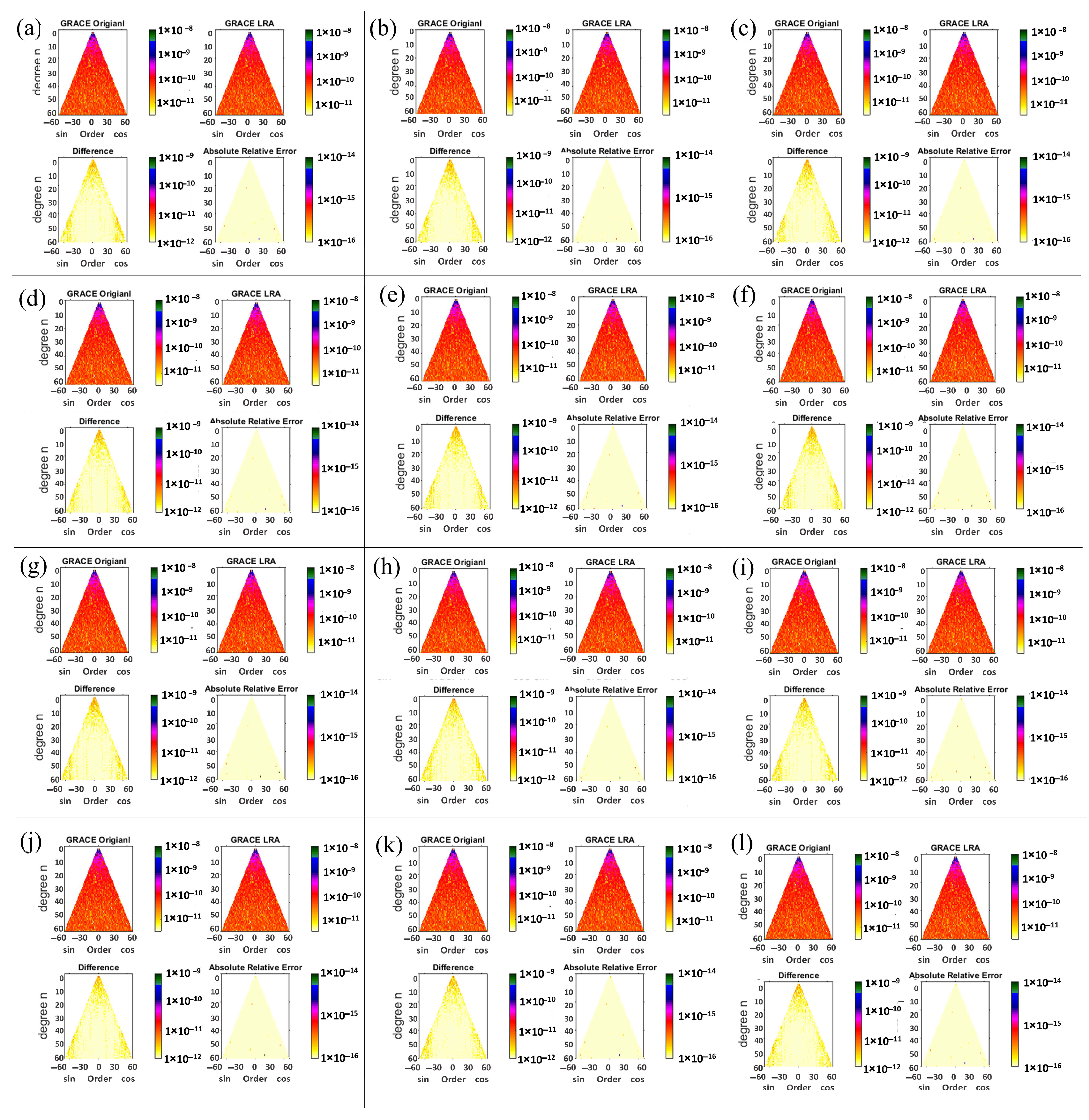
4.1.1. GRACE and LRA SHCs
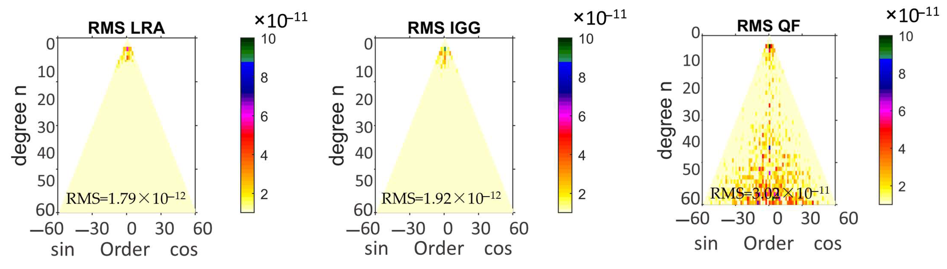
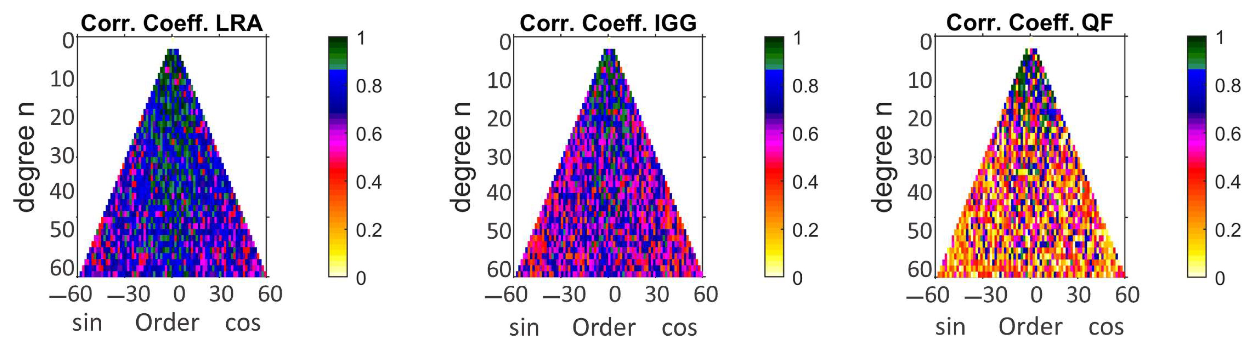
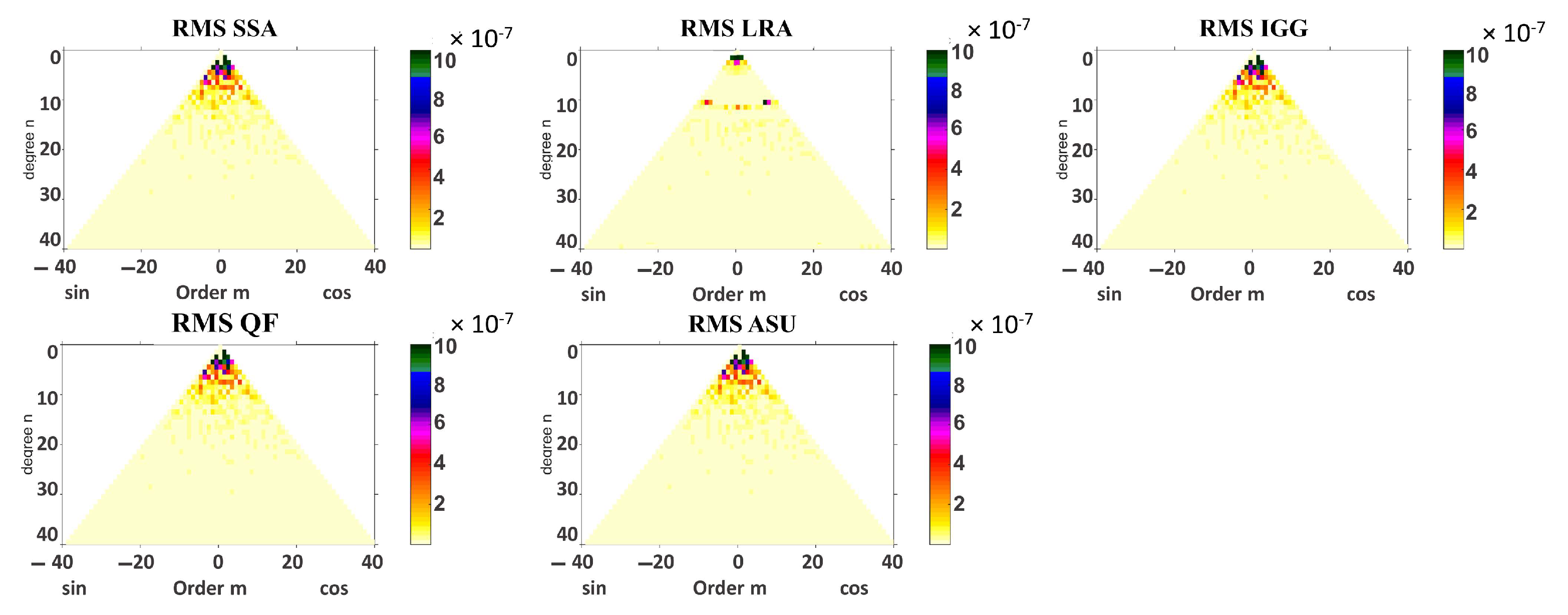
4.1.2. Validation between LRA, GRACE, QF, and IGG
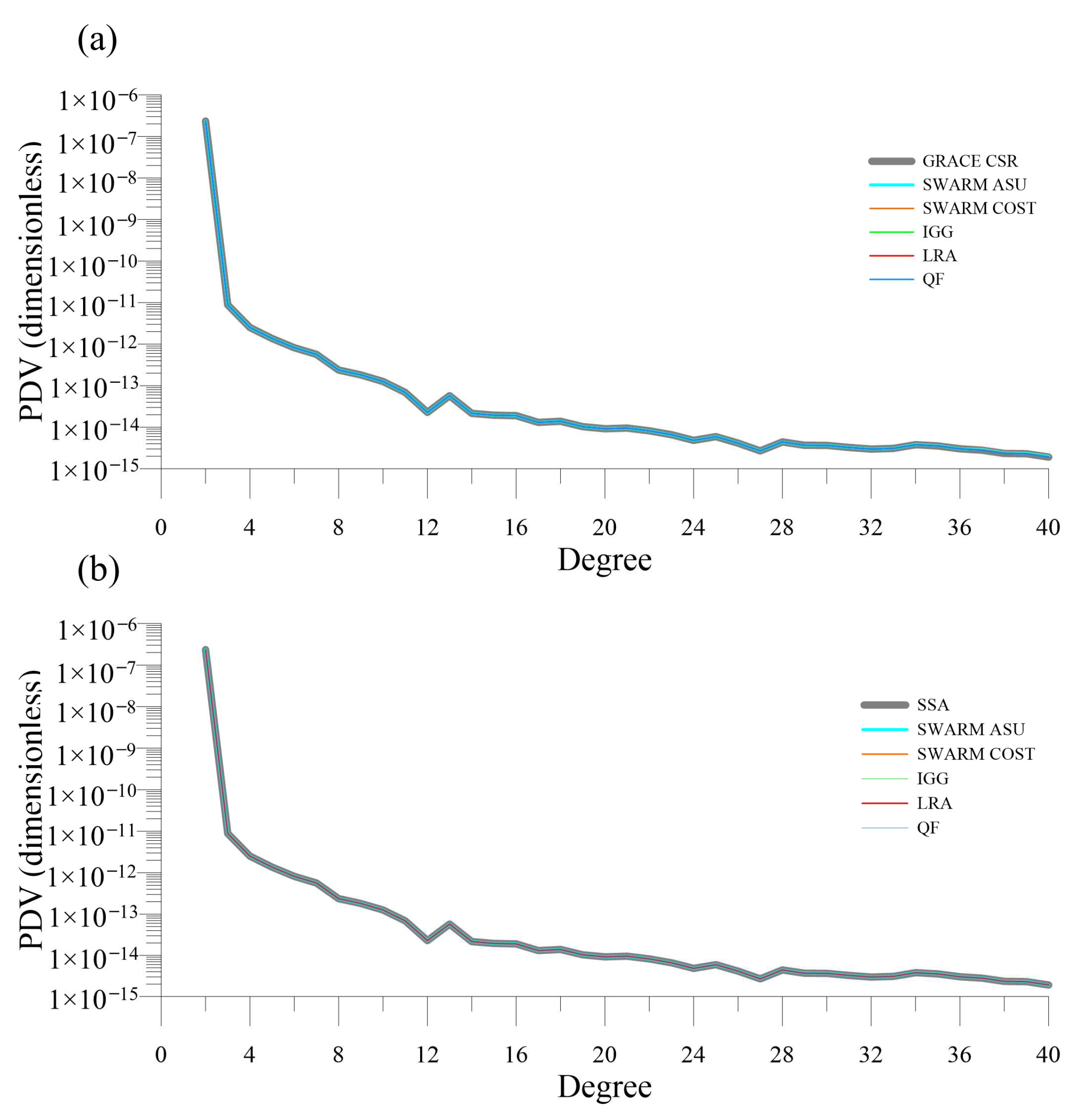
4.2. Potential Degree Variance (PDV)
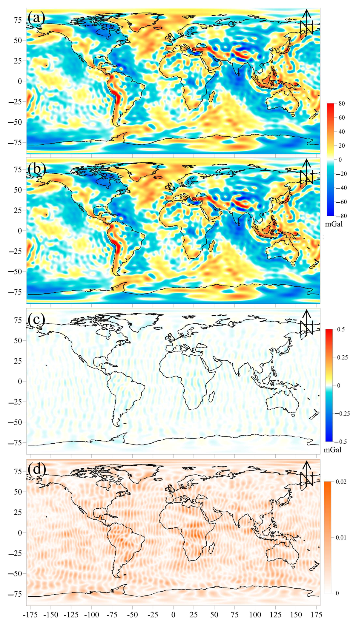
4.3. Gravity Anomaly (GA)
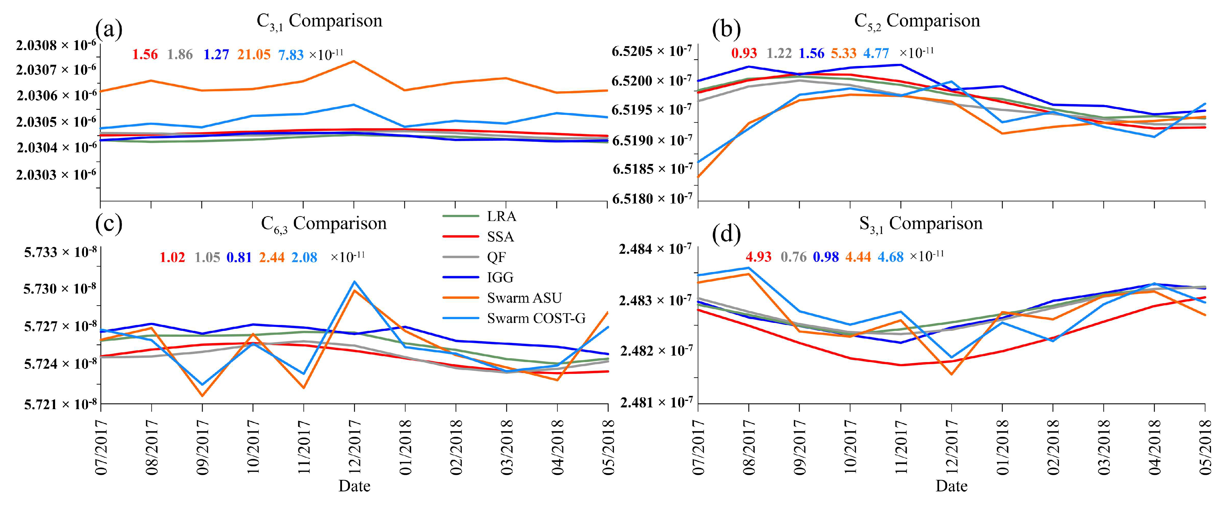
4.4. Validation between LRA and GRACE, QF, IGG, and Swarm (GRACE Gap)
5. Mascon Data Using LRA Gap-Filling Model
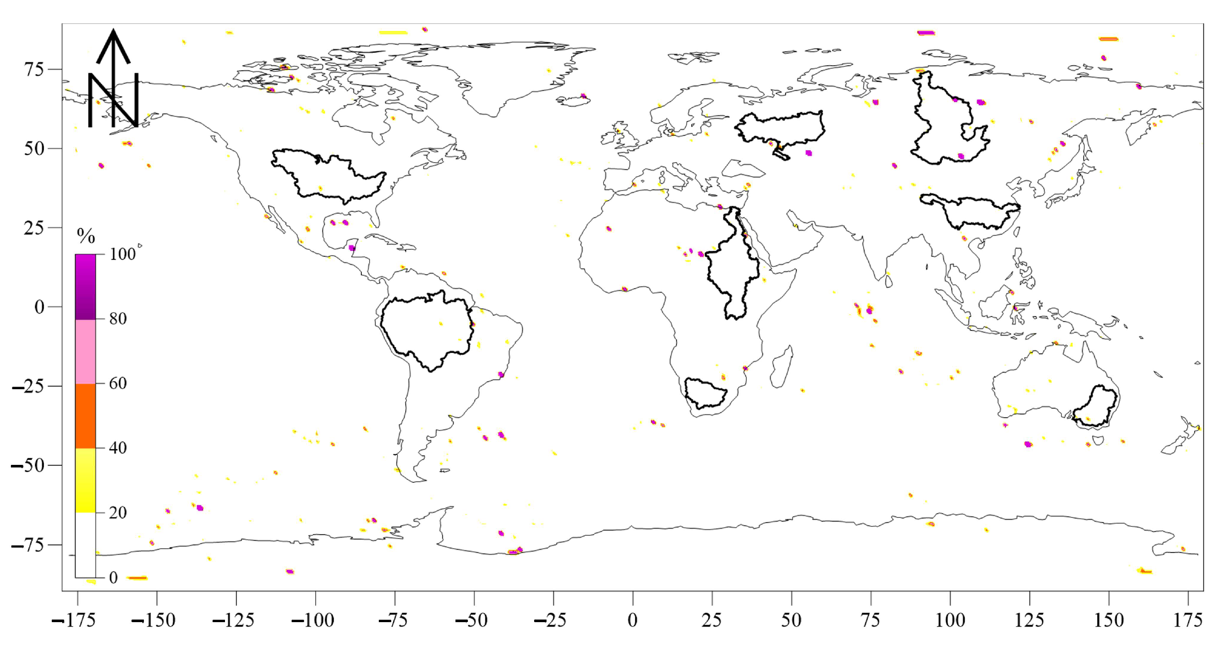
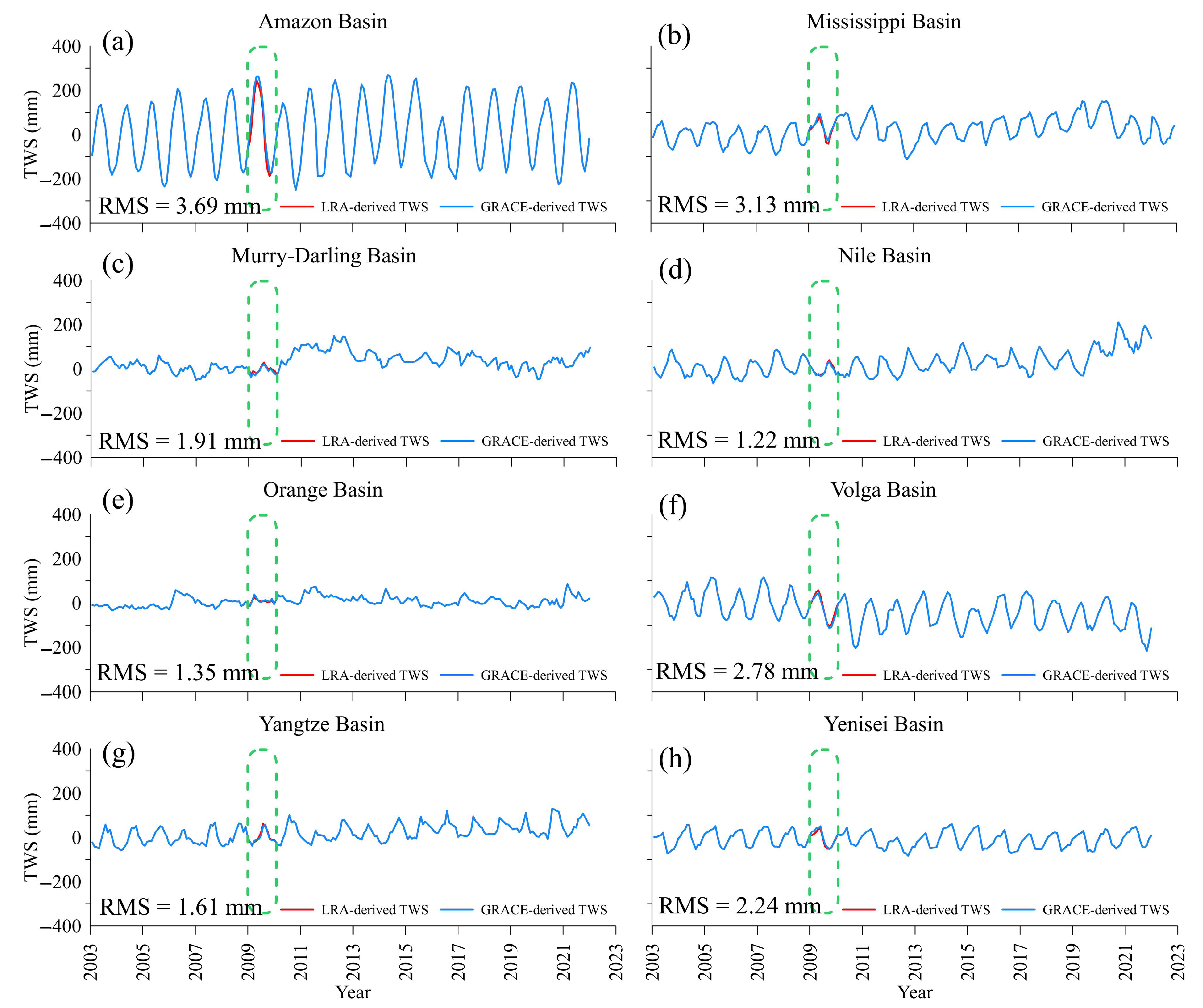
5.1. Mass Change in the Selected Basins
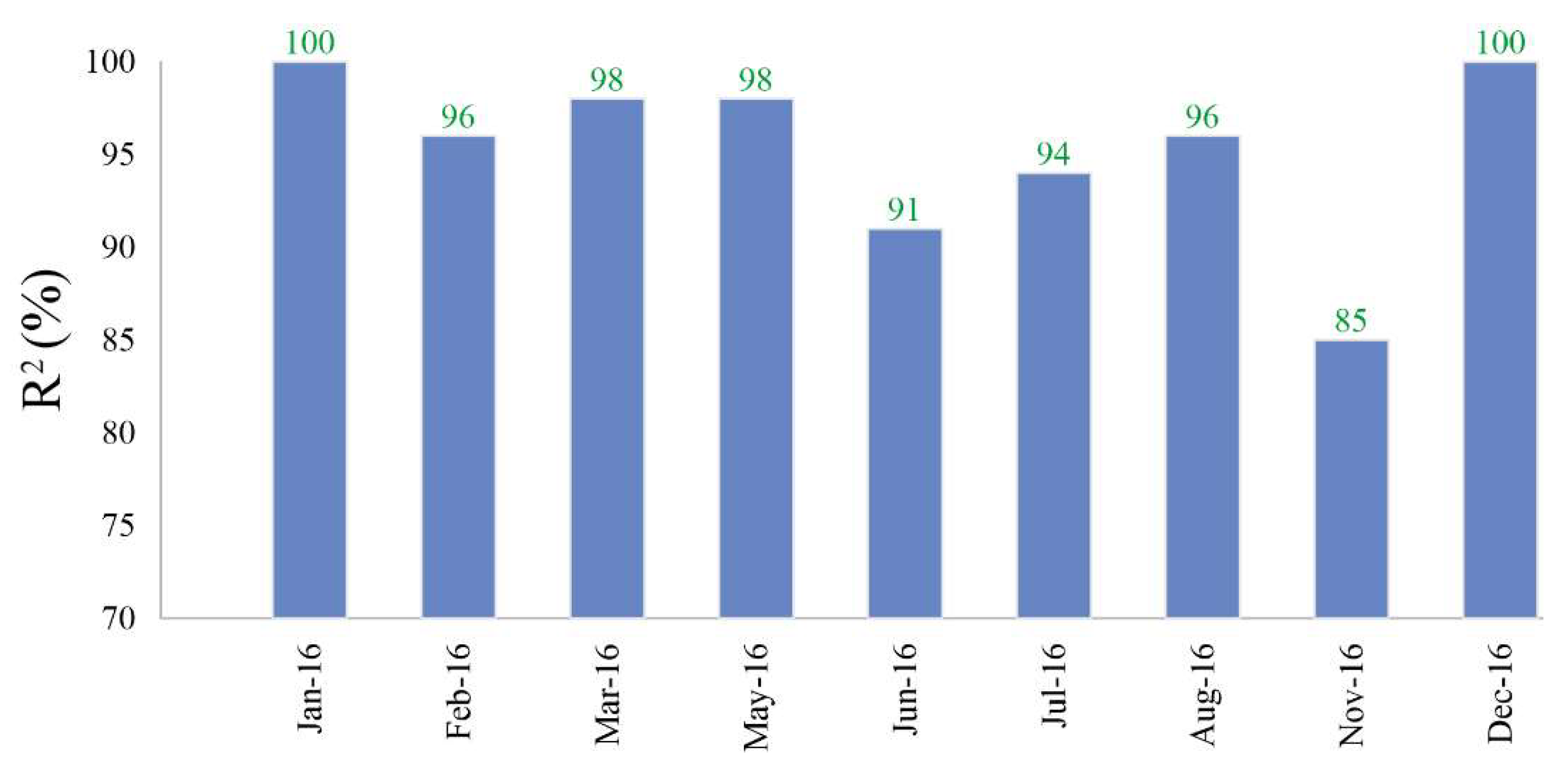
5.2. Mean Percentage Error (MPE) and Coefficient of Determination (R2)
5.3. TWS Trend
6. Conclusions
Author Contributions
Funding
Data Availability Statement
Acknowledgments
Conflicts of Interest
References
- Kornfeld, R.P.; Arnold, B.W.; Gross, M.A.; Dahya, N.T.; Klipstein, W.M.; Gath, P.F.; Bettadpur, S. GRACE-FO: The gravity recovery and climate experiment follow-on mission. J. Spacecr. Rocket. 2019, 56, 931–951. [Google Scholar] [CrossRef]
- Frappart, F.; Ramillien, G. Monitoring groundwater storage changes using the Gravity Recovery and Climate Experiment (GRACE) satellite mission: A review. Remote Sens. 2018, 10, 829. [Google Scholar] [CrossRef]
- Tapley, B.D.; Bettadpur, S.; Ries, J.C.; Thompson, P.F.; Watkins, M.M. GRACE measurements of mass variability in the Earth system. Science 2004, 305, 503–505. [Google Scholar] [CrossRef] [PubMed]
- Landerer, F.W.; Flechtner, F.M.; Save, H.; Webb, F.H.; Bandikova, T.; Bertiger, W.I.; Bettadpur, S.V.; Byun, S.H.; Dahle, C.; Dobslaw, H.; et al. Extending the global mass change data record: GRACE Follow-On instrument and science data performance. Geophys. Res. Lett. 2020, 47, e2020GL088306. [Google Scholar] [CrossRef]
- Mohasseb, H.A.; Shen, W.; Jiao, J.; Wu, Q. Groundwater Storage Variations in the Main Karoo Aquifer Estimated Using GRACE and GPS. Water 2023, 15, 3675. [Google Scholar] [CrossRef]
- Kusche, J.; Klemann, V.; Bosch, W. Mass distribution and mass transport in the Earth system. J. Geodyn. 2012, 59, 1–8. [Google Scholar] [CrossRef]
- Munagapati, H.; Tiwari, V.M. Spatio-temporal patterns of mass changes in himalayan glaciated region from EOF analyses of GRACE Data. Remote Sens. 2021, 13, 265. [Google Scholar] [CrossRef]
- Ghobadi-Far, K.; Šprlák, M.; Han, S.-C. Determination of ellipsoidal surface mass change from GRACE time-variable gravity data. Geophys. J. Int. 2019, 219, 248–259. [Google Scholar] [CrossRef]
- Liu, R.; Li, J.; Fok, H.S.; Shum, C.; Li, Z. Earth surface deformation in the north China plain detected by joint analysis of GRACE and GPS data. Sensors 2014, 14, 19861–19876. [Google Scholar] [CrossRef]
- Śliwińska, J.; Wińska, M.; Nastula, J. Preliminary estimation and validation of polar motion excitation from different types of the grace and grace follow-on missions data. Remote Sens. 2020, 12, 3490. [Google Scholar] [CrossRef]
- Pie, N.; Bettadpur, S.V.; Tamisiea, M.; Krichman, B.; Save, H.; Poole, S.; Nagel, P.; Kang, Z.; Jacob, G.; Ellmer, M.; et al. Time variable Earth gravity field models from the first spaceborne laser ranging interferometer. J. Geophys. Res. Solid Earth 2021, 126, e2021JB022392. [Google Scholar] [CrossRef]
- Li, W.; Wang, W.; Zhang, C.; Wen, H.; Zhong, Y.; Zhu, Y.; Li, Z. Bridging terrestrial water storage anomaly during GRACE/GRACE-FO gap using SSA method: A case study in China. Sensors 2019, 19, 4144. [Google Scholar] [CrossRef]
- Qian, A.; Yi, S.; Li, F.; Su, B.; Sun, G.; Liu, X. Evaluation of the Consistency of Three GRACE Gap-Filling Data. Remote Sens. 2022, 14, 3916. [Google Scholar] [CrossRef]
- Zhang, B.; Yao, Y.; He, Y. Bridging the data gap between GRACE and GRACE-FO using artificial neural network in Greenland. J. Hydrol. 2022, 608, 127614. [Google Scholar] [CrossRef]
- Zhang, X.; Li, J.; Dong, Q.; Wang, Z.; Zhang, H.; Liu, X. Bridging the gap between GRACE and GRACE-FO using a hydrological model. Sci. Total Environ. 2022, 822, 153659. [Google Scholar] [CrossRef]
- Yi, S.; Sneeuw, N. Filling the data gaps within GRACE missions using singular spectrum analysis. J. Geophys. Res. Solid Earth 2021, 126, e2020JB021227. [Google Scholar] [CrossRef]
- Lenczuk, A.; Klos, A.; Bogusz, J. Studying spatio-temporal patterns of vertical displacements caused by groundwater mass changes observed with GPS. Remote Sens. Environ. 2023, 292, 113597. [Google Scholar] [CrossRef]
- Mohasseb, H.; Abd-Elmotaal, H.A.; Shen, W. Validation of Using SWARM to Fill-in the GRACE/GRACE-FO Gap: Case Study in Africa. In Proceedings of the EGU General Assembly Conference Abstracts 2021, EGU21-2723, Virtual, 19–30 April 2021; Available online: http://www.doi.org/10.5194/egusphere-egu21-2723 (accessed on 31 December 2023).
- Richter, H.M.P.; Lück, C.; Klos, A.; Sideris, M.G.; Rangelova, E.; Kusche, J. Reconstructing GRACE-type time-variable gravity from the Swarm satellites. Sci. Rep. 2021, 11, 1–14. [Google Scholar] [CrossRef] [PubMed]
- Forootan, E.; Schumacher, M.; Mehrnegar, N.; Bezděk, A.; Talpe, M.J.; Farzaneh, S.; Zhang, C.; Zhang, Y.; Shum, C.K. An iterative ICA-based reconstruction method to produce consistent time-variable total water storage fields using GRACE and Swarm satellite data. Remote Sens. 2020, 12, 1639. [Google Scholar] [CrossRef]
- Wang, F.; Shen, Y.; Chen, Q.; Wang, W. Bridging the gap between GRACE and GRACE follow-on monthly gravity field solutions using improved multichannel singular spectrum analysis. J. Hydrol. 2021, 594, 125972. [Google Scholar] [CrossRef]
- da Encarnacao, J.T.; Visser, P.; Arnold, D.; Bezdek, A.; Doornbos, E.; Ellmer, M.; Guo, J.; Ijssel, J.v.D.; Iorfida, E.; Jäggi, A.; et al. Description of the multi-approach gravity field models from Swarm GPS data. Earth Syst. Sci. Data 2020, 12, 1385–1417. [Google Scholar] [CrossRef]
- Zhong, B.; Li, X.; Chen, J.; Li, Q.; Liu, T. Surface Mass Variations from GPS and GRACE/GFO: A Case Study in Southwest China. Remote Sens. 2020, 12, 1835. [Google Scholar] [CrossRef]
- Matsuo, K.; Chao, B.F.; Otsubo, T.; Heki, K. Accelerated ice mass depletion revealed by low-degree gravity field from satellite laser ranging: Greenland, 1991–2011. Geophys. Res. Lett. 2013, 40, 4662–4667. [Google Scholar] [CrossRef]
- Bloßfeld, M.; Müller, H.; Gerstl, M.; Štefka, V.; Bouman, J.; Göttl, F.; Horwath, M. Second-degree Stokes coefficients from multi-satellite SLR. J. Geod. 2015, 89, 857–871. [Google Scholar] [CrossRef]
- Sośnica, K.; Jäggi, A.; Meyer, U.; Thaller, D.; Beutler, G.; Arnold, D.; Dach, R. Time variable Earth’s gravity field from SLR satellites. J. Geod. 2015, 89, 945–960. [Google Scholar] [CrossRef]
- Uz, M.; Atman, K.G.; Akyilmaz, O.; Shum, C.; Keleş, M.; Ay, T.; Tandoğdu, B.; Zhang, Y.; Mercan, H. Bridging the gap between GRACE and GRACE-FO missions with deep learning aided water storage simulations. Sci. Total Environ. 2022, 830, 154701. [Google Scholar] [CrossRef]
- Chu, J.; Su, X.; Jiang, T.; Qi, J.; Zhang, G.; Wu, H. Filling the gap between GRACE and GRACE-FO data using a model integrating variational mode decomposition and long short-term memory: A case study of Northwest China. Environ. Earth Sci. 2023, 82, 1–16. [Google Scholar] [CrossRef]
- Gyawali, B.; Ahmed, M.; Murgulet, D.; Wiese, D.N. Filling Temporal Gaps within and between GRACE and GRACE-FO Terrestrial Water Storage Records: An Innovative Approach. Remote Sens. 2022, 14, 1565. [Google Scholar] [CrossRef]
- Sun, Z.; Long, D.; Yang, W.; Li, X.; Pan, Y. Reconstruction of GRACE data on changes in total water storage over the global land surface and 60 basins. Water Resour. Res. 2020, 56, e2019WR026250. [Google Scholar] [CrossRef]
- Li, F.; Kusche, J.; Rietbroek, R.; Wang, Z.; Forootan, E.; Schulze, K.; Lück, C. Comparison of data-driven techniques to reconstruct (1992–2002) and predict (2017–2018) GRACE-like gridded total water storage changes using climate inputs. Water Resour. Res. 2020, 56, e2019WR026551. [Google Scholar] [CrossRef]
- Lenczuk, A.; Weigelt, M.; Kosek, W.; Mikocki, J. Autoregressive Reconstruction of Total Water Storage within GRACE and GRACE Follow-On Gap Period. Energies 2022, 15, 4827. [Google Scholar] [CrossRef]
- Karimi, H.; Iran-Pour, S.; Amiri-Simkooei, A.; Babadi, M. A gap-filling algorithm selection strategy for GRACE and GRACE Follow-On time series based on hydrological signal characteristics of the individual river basins. J. Geod. Sci. 2023, 13, 2023. [Google Scholar] [CrossRef]
- Wiese, D.N.; Landerer, F.W.; Watkins, M.M. Quantifying and reducing leakage errors in the JPL RL05M GRACE mascon solution. Water Resour. Res. 2016, 52, 7490–7502. [Google Scholar] [CrossRef]
- Save, H.; Bettadpur, S.; Tapley, B.D. High-resolution CSR GRACE RL05 mascons. J. Geophys. Res. Solid Earth 2016, 121, 7547–7569. [Google Scholar] [CrossRef]
- Wahr, J.; Molenaar, M.; Bryan, F. Time variability of the Earth’s gravity field: Hydrological and oceanic effects and their possible detection using GRACE. J. Geophys. Res. Solid Earth 1998, 103, 30205–30229. [Google Scholar] [CrossRef]
- Chen, J.; Tapley, B.; Tamisiea, M.E.; Save, H.; Wilson, C.; Bettadpur, S.; Seo, K.-W. Error Assessment of GRACE and GRACE Follow-On Mass Change. J. Geophys. Res. Solid Earth 2021, 126, e2021JB022124. [Google Scholar] [CrossRef]
- Swenson, S.; Famiglietti, J.; Basara, J.; Wahr, J. Estimating profile soil moisture and groundwater variations using GRACE and Oklahoma Mesonet soil moisture data. Water Resour. Res. 2008, 44, W01413. [Google Scholar] [CrossRef]
- Löcher, A.; Kusche, J. A hybrid approach for recovering high-resolution temporal gravity fields from satellite laser ranging. J. Geod. 2020, 95, 6. [Google Scholar] [CrossRef]
- Weigelt, M. Time Series of Monthly Combined HLSST and SLR Gravity Field Models to Bridge the Gap between GRACE and GRACE-FO: QuantumFrontiers_HLSST_SLR_COMB2019s; GFZ Data Services; GFZ: Potsdam, Germany, 2019. [Google Scholar] [CrossRef]
- Gillard, J. An overview of linear structural models in errors in variables regression. REVSTAT-Stat. J. 2010, 8, 57–80. [Google Scholar] [CrossRef]
- Tranmer, M.; Elliot, M. Multiple linear regression. Cathie Marsh Cent. Census Surv. Res. (CCSR) 2008, 5, 1–5. [Google Scholar]
- Casson, R.J.; Farmer, L.D. Understanding and checking the assumptions of linear regression: A primer for medical researchers. Clin. Exp. Ophthalmol. 2014, 42, 590–596. [Google Scholar] [CrossRef] [PubMed]
- Zou, K.H.; Tuncali, K.; Silverman, S.G. Correlation and simple linear regression. Radiology 2003, 227, 617–628. [Google Scholar] [CrossRef] [PubMed]
- Laurent, R.T.S. Understanding Regression Assumptions; Taylor & Francis: Abingdon, UK, 1994. [Google Scholar]
- Berry, W.D. Understanding Regression Assumptions; Sage: New York, NY, USA, 1993. [Google Scholar] [CrossRef]
- Cui, L.; Song, Z.; Luo, Z.; Zhong, B.; Wang, X.; Zou, Z. Comparison of terrestrial water storage changes derived from GRACE/GRACE-FO and Swarm: A case study in the Amazon River Basin. Water 2020, 12, 3128. [Google Scholar] [CrossRef]
- Heiskanen, W.A.; Moritz, H. Physical Geodesy; Springer: Berlin/Heidelberg, Germany, 1967. [Google Scholar] [CrossRef]
- Vanicek, P.; Krakiwsky, E.J. Geodesy: The Concepts; Elsevier: Amsterdam, The Netherlands, 2015. [Google Scholar]
- Tscherning, C. Determination of sea surface topography from satellite radar altimetry [ocean geoid, ocean circulation, altimeter]. In Conference on Satellite Based Navigation and Remote Sensing of the Sea, Copenhagen (Denmark), 4 Mar 1980; DDNIUGG: Ottawa, ON, Canada, 1980. [Google Scholar]
- Wolf, P.R.; Ghilani, C.D. Adjustment Computations Spatial Data Analysis; John Wiley: Hoboken, NJ, USA, 2006. [Google Scholar]
- Ghilani, C.D. Adjustment Computations: Spatial Data Analysis; John Wiley & Sons: Hoboken, NJ, USA, 2017. [Google Scholar]


| Basin | Approximate Area (km2) | Location |
|---|---|---|
| Nile basin | 3,038,100 | East and North Africa |
| Orange basin | 850,000 | Southern Africa |
| Mississippi basin | 2,980,000 | North America |
| Amazon basin | 5,500,000 | South America |
| Volga basin | 1,360,000 | Europe |
| Yenisei basin | 2,580,000 | Asia |
| Yangtze basin | 1,800,000 | Asia |
| Murray Darling basin | 1,061,469 | Australia |
| Source | Correlation Coefficients |
|---|---|
| LRA | 0.8258 |
| IGG | 0.6763 |
| QF | 0.5428 |
| Basin | Terrestrial Water Storage (mm) | ||
|---|---|---|---|
| GRACE | LRA | GRACE-LRA | |
| Amazon | 5.53 | 6.48 | 5.14 |
| Mississippi | 1.18 | 1.53 | 0.78 |
| Murry-Darling | 0.42 | 0.64 | 0.45 |
| Nile | 1.82 | 1.34 | 0.64 |
| Orange | 0.41 | 0.54 | 0.58 |
| Volga | 1.69 | 1.05 | 0.96 |
| Yangtze | 1.62 | 0.97 | 1.05 |
| Yenisei | 1.31 | 1.08 | 0.65 |
| Month | ) | Standard Deviation (σ) | Variance (1/σ2) | |||
|---|---|---|---|---|---|---|
| GRACE | LRA | GRACE | LRA | GRACE | LRA | |
| January | −0.653 | −0.701 | 6.415 | 6.869 | 0.0243 | 0.0212 |
| February | −0.447 | −0.526 | 6.817 | 7.071 | 0.0215 | 0.0200 |
| March | −0.580 | −0.483 | 7.618 | 7.920 | 0.0172 | 0.0159 |
| April | −0.396 | −0.348 | 7.819 | 7.593 | 0.0164 | 0.0173 |
| May | 0.018 | 0.164 | 8.098 | 8.117 | 0.0152 | 0.0152 |
| June | 0.315 | 0.316 | 7.819 | 8.070 | 0.0164 | 0.0154 |
| July | 0.126 | −0.089 | 7.902 | 8.042 | 0.0160 | 0.0155 |
| August | −0.134 | −0.184 | 9.149 | 9.281 | 0.0119 | 0.0116 |
| September | −0.290 | −0.217 | 9.698 | 9.545 | 0.0106 | 0.0110 |
| October | −0.225 | −0.506 | 9.666 | 9.441 | 0.0107 | 0.0112 |
| November | −0.556 | −0.564 | 9.542 | 9.158 | 0.0110 | 0.0119 |
| December | −0.707 | −0.734 | 8.949 | 9.218 | 0.0125 | 0.0118 |
| Source | Weighted Mean | Standard Deviation of the Weighted Mean |
|---|---|---|
| GRACE/GRACE-FO | −0.308 | 1.047 |
| LRA | −0.329 | 1.149 |
| Basin | TWS Trend (mm/year) | |
|---|---|---|
| Using LRA | Without LRA | |
| Amazon | 2.17 ±0.15 | 2.21 ±0.16 |
| Mississippi | 3.43 ± 0.22 | 3.65 ± 0.21 |
| Murry Darling | 1.74 ± 0.13 | 1.75 ± 0.13 |
| Nile | 4.94 ± 0.25 | 5.06 ± 0.23 |
| Orange | 0.94 ± 0.36 | 0.94 ± 0.37 |
| Volga | −4.47 ± 0.30 | −4.53 ± 0.28 |
| Yangtze | 3.49 ± 0.32 | 3.52 ± 0.30 |
| Yenisei | −0.56 ± 0.05 | −0.53 ± 0.05 |
Disclaimer/Publisher’s Note: The statements, opinions and data contained in all publications are solely those of the individual author(s) and contributor(s) and not of MDPI and/or the editor(s). MDPI and/or the editor(s) disclaim responsibility for any injury to people or property resulting from any ideas, methods, instructions or products referred to in the content. |
© 2024 by the authors. Licensee MDPI, Basel, Switzerland. This article is an open access article distributed under the terms and conditions of the Creative Commons Attribution (CC BY) license (https://creativecommons.org/licenses/by/4.0/).
Share and Cite
Mohasseb, H.A.; Shen, W.; Jiao, J. Monsoon-Based Linear Regression Analysis for Filling Data Gaps in Gravity Recovery and Climate Experiment Satellite Observations. Remote Sens. 2024, 16, 1424. https://doi.org/10.3390/rs16081424
Mohasseb HA, Shen W, Jiao J. Monsoon-Based Linear Regression Analysis for Filling Data Gaps in Gravity Recovery and Climate Experiment Satellite Observations. Remote Sensing. 2024; 16(8):1424. https://doi.org/10.3390/rs16081424
Chicago/Turabian StyleMohasseb, Hussein A., Wenbin Shen, and Jiashuang Jiao. 2024. "Monsoon-Based Linear Regression Analysis for Filling Data Gaps in Gravity Recovery and Climate Experiment Satellite Observations" Remote Sensing 16, no. 8: 1424. https://doi.org/10.3390/rs16081424
APA StyleMohasseb, H. A., Shen, W., & Jiao, J. (2024). Monsoon-Based Linear Regression Analysis for Filling Data Gaps in Gravity Recovery and Climate Experiment Satellite Observations. Remote Sensing, 16(8), 1424. https://doi.org/10.3390/rs16081424