Abstract
This paper investigates the airborne synthetic aperture radar via outfield experiments based on carrier-free ultra-wideband signals with fifth-order Gaussian pulses with imaging using the backward projection algorithm. Typical blanket jamming is selected in the study, and NAM, NFM, and SFM are used as jamming signals to investigate the backward projection BP imaging effect of airborne synthetic aperture radar when subjected to blanket jamming in a real-world environment. Subsequently, a variational modal decomposition algorithm is proposed, aiming at the anti-jamming processing of airborne synthetic aperture radar. Further, the variational modal decomposition algorithms are compared with the empirical modal decomposition for the anti-jamming effect, which verified the effectiveness and high efficiency of the method. This study provides a new solution for the imaging problem of airborne synthetic aperture radar when subjected to blanket jamming, and a helpful reference is provided for the selection of anti-jamming processing methods.
1. Introduction
With the continuous development of science and technology, synthetic aperture radar (SAR) has become an important remote sensing technology with increasingly diverse applications. Various new SAR technologies have emerged, such as multi-channel high-resolution and wide-band SAR (HRWS), multi-baseline interferometric SAR, multi-sub-band SAR, and polarimetric SAR (PolSAR) and polarimetric interferometric SAR (PolInSAR) [1]. These new SAR systems demonstrate significant advantages in imaging quality, target identification capability, and information extraction. The use of SAR is becoming increasingly widespread in applications such as oil spill detection, terrain mapping, etc. [2,3,4]. However, with the diversification of SAR application scenarios, the jamming issues faced by SAR systems have become increasingly complex. Traditional anti-jamming processing methods often fail to meet the requirements of new SAR systems, making research and improvement in SAR anti-jamming processing particularly urgent and necessary [5,6,7,8,9,10,11,12,13].
Blanket jamming, as a typical form of jamming, uses high-power noise signals to suppress the normal reception of radar signals and consequently submerge the real targets in SAR images. Therefore, effectively dealing with suppressive jamming has become a crucial issue in SAR anti-jamming research. With the continuous development of technology, many methods have emerged to address this problem. These methods are used to improve the robustness and anti-jamming ability of SAR systems when facing suppressive jamming. Through continuous exploration and innovation, it is possible to better ensure the normal operation of SAR systems, ensuring the accurate and reliable imaging and detection of targets [14,15,16,17,18].
In reference [14], an anti-jamming method for identifying stationary false targets is proposed. This method is based on the dynamic characteristics of frequency shift deception jamming and utilizes Displaced Phase Center Antenna (DPCA) processing. It can display stationary false targets and indicate their positions in SAR images. This method is applicable to dynamic disturbances and static targets, with significant requirements on the states of the disturbances and targets. In reference [15], an anti-jamming method for generating LFM-PC signals using orthogonal phase-coded signals with different pulse repetition intervals (PRIs) is proposed. Reference [16] proposes an anti-jamming method for SAR based on the distance-Doppler algorithm, which combines waveform modulation and azimuth misalignment filtering. In reference [17], a method for anti-jamming in MIMO-SAR is proposed, which is based on azimuth phase coding (APC) and orthogonal frequency-division multiplexing (OFDM) dual modulation. Methods [15,16,17] all involve the complex processing of radar transmission signals beyond the basic radar emissions. However, these methods are only effective against deceptive jamming, utilizing the differences between deceptive jamming and certain characteristics of the transmission signal for anti-jamming purposes. There are some limitations to this approach. In reference [18], a phase jitter optimization model based on linear frequency-modulated signals is proposed, allowing the phase jitter of the signal to be optimized in three degrees of freedom. This method utilizes the inherent characteristics of the signal to counter deceptive interference based on phase changes in three degrees of freedom. However, although these methods are effective against deceptive interference, they may not necessarily be effective in more complex scenarios.
The variational modal decomposition (VMD) algorithm is a signal decomposition algorithm proposed with the inspiration of empirical modal decomposition, but in essence, it is entirely different from empirical modal decomposition (EMD). In 2014, Professors Konstantin Dragomiretskiy and Dominique Zosso proposed the variational modal decomposition algorithm based on the theoretical foundation of the EMD algorithm [19]. The VMD algorithm is essentially an extension of the classical Wiener filtering to decompose over multiple bands adaptively and adopt an iterative approach to solve the optimal solution of the variational modes. The basic idea of the VMD algorithm is to iteratively decompose the original signal into multiple IMF components, each of which has a specific center frequency and finite bandwidth, and then to decompose the practical components corresponding to each center frequency in the frequency domain. In the past, the VMD algorithm was often used for fault diagnosis [20,21,22].
In this paper, a VMD method is used for the anti-jamming process. The VMD algorithm decomposes the signal into several different IMF components and reconstructs the desired signal components from them to produce an anti-jamming signal. The VMD algorithm starts from the frequency domain, without considering the states of the target and radar, or the types of jamming signals. As long as the jamming signal and the target signal are at different frequencies, the target signal can be decomposed from the jamming signal. It is compared with the empirical modal decomposition to demonstrate the effectiveness of VMD anti-jamming. Such a study helps to improve the imaging quality and accuracy of SAR systems in complex environments and provides more reliable technical support for practical applications.
2. Carrier-Free Ultra-Wideband Signal
Ultra-wideband pulsed signals are usually a class of signals with very short durations containing rich frequency components. They can be used as ultra-wideband pulses when the signals satisfy their relative bandwidths. Ideal impulse functions are difficult to achieve, and the following are the primary forms of commonly used ultra-wideband impulse signals: multi-periodic impulse signals, ascending cosine impulses, and Gaussian impulses, among which Gaussian impulses are one of the most used waveforms. The fundamental (zero-order) Gaussian signal can be expressed as
where is the mean square deviation of the signal, also known as the pulse width factor. The power spectrum of the Gaussian signal in Equation (1) can be expressed as
The energy of the primary Gaussian signal is mainly concentrated in the low-frequency range, and the closer the frequency is to zero, the greater the power, which is unsuitable for wireless transmission. Therefore, the differential form of the Gaussian signal is generally chosen as the ultra-wideband pulse signal. The primary Gaussian signal with its 1–5 times differential form is shown in Equation (3).
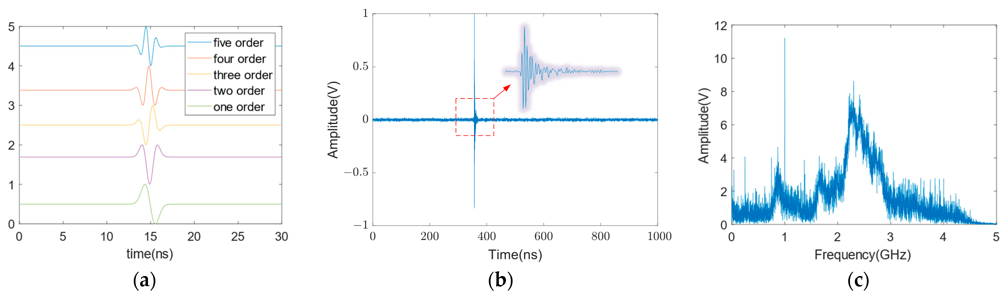
The in Equation (3) represents the amplitude of the Gaussian pulse. The time-domain waveform corresponding to the fundamental Gaussian signal 1–5th differential is shown in Figure 1a.
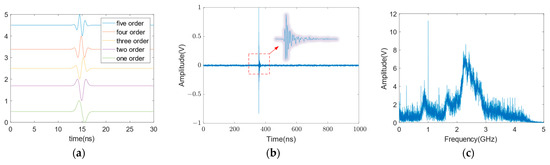
Figure 1.
Carrier-free ultra-wideband signals. (a) Gaussian signals of orders 1–5; (b) Time-domain signal of 5th-order Gaussian; (c) Spectrogram of 5th-order Gaussian.
All subsequent analyses in this paper use 5th-order Gaussian pulses collected in the laboratory with a pulse width of about 5 ns and a preset sampling frequency of 10 GHz. The time-domain waveforms and spectra of the fifth-order Gaussian pulses normalized with a single amplitude are shown in Figure 1b. As can be seen from Figure 1c, the center of the spectrum of the fifth-order Gaussian pulse under this condition is 2.3 GHz.
3. Backward Projection Imaging
3.1. Airborne SAR Imaging Model
Carrier-free ultra-wideband SAR is generally mounted on carriers such as UAVs, aircraft, satellites, etc. In addition to receiving direct echo signals when the airline of the SAR is flying at a certain speed, multiple echo signals from the same target can also be received. The SAR system can obtain high-resolution images by synthesizing multiple signals from different locations. In this paper, we take the airborne strip synthetic aperture radar as an example and establish an echo imaging model for SAR. The spatial geometry model between the airborne SAR and the target is shown in Figure 2.
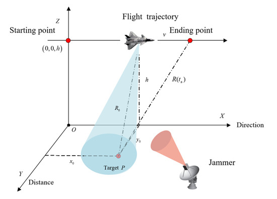
Figure 2.
Airborne SAR imaging model.
The carrier platform flies along the azimuthal direction with a sure speed of in a uniform, straight line, and the height of the radar platform is . Then, at the moment , the platform coordinates can be expressed as , and is the distance from the platform to the center of the observation belt. The SAR antenna illuminates the observation area and collects the echo data during the movement. Taking the point target P on the imaging belt as an example, assuming its coordinates are , the instantaneous slant distance between the SAR and the target P at the moment can be expressed as
Assuming that the target is an ideal point target, the received point target echo signal can be expressed as
where denotes the pulse amplitude; denotes the emitted signal, in this case, a 5th-order Gaussian pulse normalized to amplitude; is the propagation speed of the electromagnetic wave through the air; and denotes clutter or jamming.
3.2. Principle of Backward Projection Algorithm
The BP algorithm is a classical time-domain algorithm, first introduced by McCorkle in 1991 in ultra-wideband pulsed SAR imaging processing [23]. The BP algorithm is simple in structure, robust, and accurate, and its core idea is to reconstruct the pixel points on the grid of the imaging region along the diagonal distance course. The echo received by the SAR is the sum of the echoes from all the scattering points and, thus, the imaging region can be dissected into a grid at regular intervals, and the SAR echo data corresponding to each aperture are back-projected onto all pixel points. At each azimuthal moment, the two-way echo time delay is obtained separately for the distance from each pixel point to the SAR, based on which the corresponding echo intensity is extracted from the echo signals, the echo signals are time-aligned and then summed up, and finally, the signals are back-projected onto the grid. Since each pixel point in the imaging area is processed and the algorithm, in principle, does not perform any approximation processing, a high resolution can be obtained.
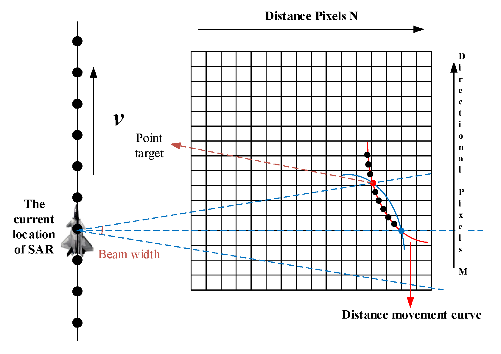
The imaging schematic of the BP algorithm is shown in Figure 3. The size of the imaging area is , indicates the number of grid pixels in the azimuth direction, shows the number of grid pixels in the distance direction, the flight speed of the airborne SAR platform is , and the location of the red point target in the figure is , which indicates that the target is located in the pixel point in the imaging area. The red curve is the distance migration curve of the point target, and the airborne SAR just sweeps to the point target when it moves to the blue position.
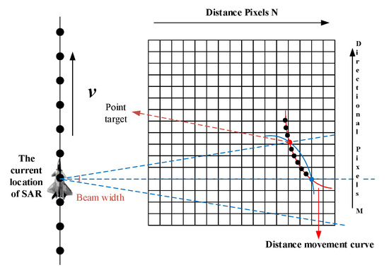
Figure 3.
The imaging schematic of the BP algorithm.
The instantaneous slant distance from the pixel point to the phase center of the radar antenna at the moment of the current bearing can be calculated according to Equation (4), and represents the two-way delay between the SAR airborne platform and the pixel point at this time.
For pixel points in the imaging area that are at the same distance from the airborne SAR, they have the same time delay to the start point of the echo signal sampling and, therefore, they move the same distance on the up-sampled data. The process of superimposing the echo with the previous azimuth to that pixel point is shown in Figure 3 as the black dots on the distance migration curve will be superimposed to the red dots, and after superimposition, the data from the point target will move to the nearest grid at the blue curve at equal distance from the radar. It then switches to the next azimuth to continue the movement, coherently accumulating for each pixel point. Each movement of the radar in the azimuthal direction will accumulate the echo signal of the point target once at the position of the red dot, while the other positions will only collect it once. Coherent accumulation makes the amplitude of the red dot position more prominent and more significant, and the difference between the amplitude of the grid points of the non-point target and the amplitude of the red dot position becomes bigger and bigger, and finally, the total energy value of the pixel point’s echo is calculated, and the image of the point can be mapped out.
The relative motion between the SAR system and the target results in a bending of the distance migration curve, so the positions of the target points in the SAR image are not their actual geographic locations. When performing distance processing, the SAR system performs distance compression on the received echo signal to remap it to the correct location. The distance to pulse compression based on a matched filter is carried out on the received echo signal; the matched filter performs a cross-correlation calculation with the received echo signal based on the known shape of the transmitted signal, and the nearest distance is used as the reference point to obtain the distance to the compressed echo data.
where is time-reversal conjugate of for a fast time convolution, target points at different distances have different curvatures of their migratory trajectories due to the differences in their relative positions to the radar system, so the targets must be focused separately. The BP algorithm achieves high-resolution imaging by calculating the distance from each pixel point to each antenna position in the imaging grid and performing time-domain coherent superposition and, thus, can meet the focusing requirements. The final image data of the imaging grid are obtained via time-domain coherent accumulation.
3.3. Carrier-Free Ultra-Wideband Airborne SAR Outfield Test Realization for Backward Projection Imaging
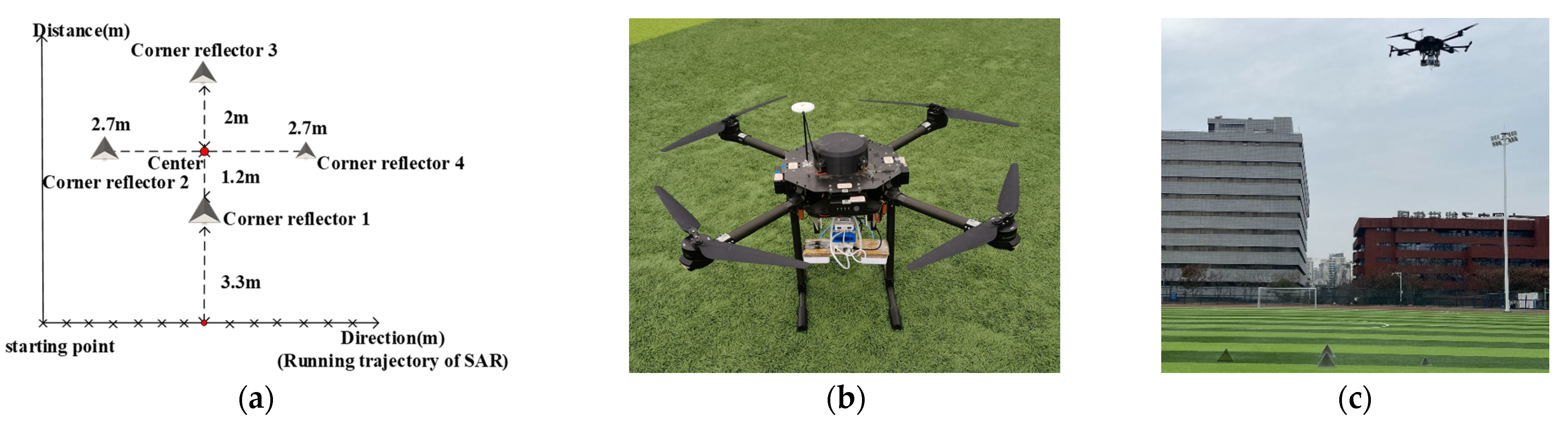
The carrier-free ultra-wideband airborne SAR system mainly consists of a small ultra-wideband SAR detection module, an uncrewed aerial vehicle (UAV), a mobile signal power supply, a wireless transmission module, and a pair of transceiver antennae. Four corner reflectors were used as experimental targets. The volume of the corner reflector 1 is slightly more prominent, and the volume of the corner reflector 4 is smaller than the others. The experimental parameters and experimental scenario design are shown in Figure 4.
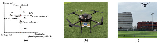
Figure 4.
Field experiment scene. (a) Experimental scenario design diagram; (b) carrier-free ultra-wideband airborne SAR; (c) airborne SAR detects target.
The experimental scenario in Figure 4 shows that the carrier-free ultra-wideband airborne SAR system scans the target along the azimuth direction. It receives echoes, and the target is always kept stationary during the experiment. The flight altitude of the UAV is 6.2 m. Figure 5 demonstrates the echo results acquired by the SAR receiving antenna.
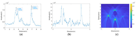
Figure 5.
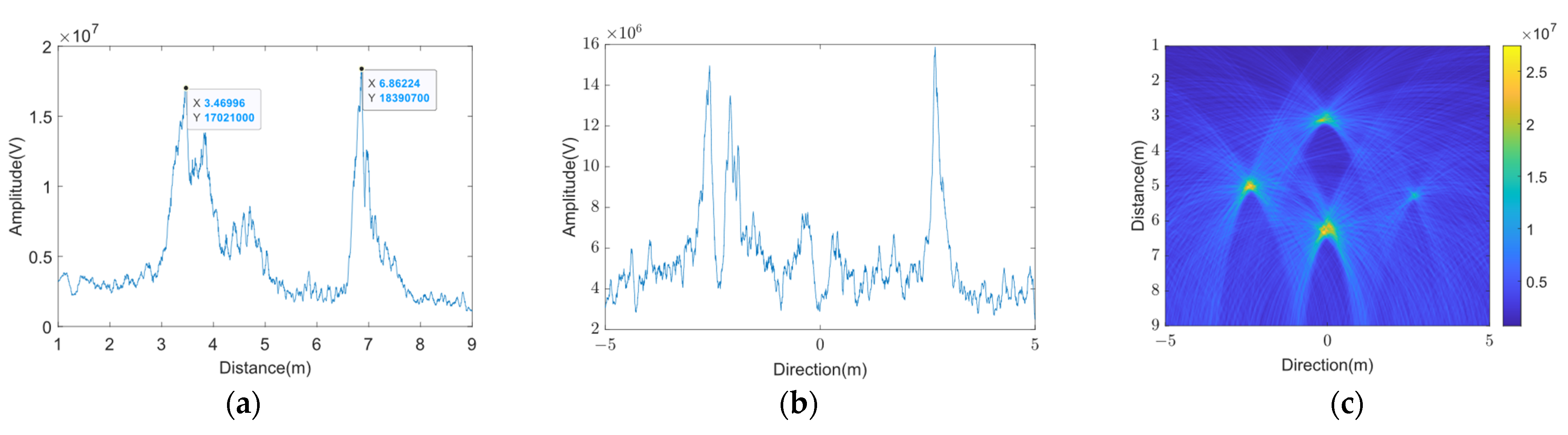
The result of field experiment. (a) Distance result; (b) Direction result; (c) Result of BP algorithm.
From the azimuthal peak profile in Figure 5b, two and four echo signals can be observed in the corner reflectors. The waveform shows that the distance between corner reflector two and the scene’s center is near 2.572 m, which is less different from the preset 2.7 m; the distance between corner reflector four and the center is 2.679 m, which is close to the actual distance. From the distance-to-peak profile in Figure 5a, it can be seen that the distances of corner reflector one and corner reflector three from the center of the scene are 3.469 m and 6.862 m. According to the analysis of the experimental data, a measurement error of about 0.36 m is generated in the echo signal of corner reflector three. This is because the distance between corner reflector three and the UAV is far; the echo signal is affected by the air medium, reflection, and other factors in the propagation process, resulting in signal propagation delay; and the delay time introduces a specific measurement error. In addition, it is challenging to avoid jitter during the flight of the UAV, and the grass environment where the experiment was conducted has complex scattering characteristics, which include factors such as the structure, humidity, and density of the grass. These factors lead to minor clutter jamming in the received SAR echo signals. The comprehensive experimental results show that the actual distance of the corner reflector and the experimental preset error are within an acceptable range. Hence, the echo data measured in this experiment were highly accurate.
The SAR echo signals acquired using the ultra-wideband detection module are imaged using the BP algorithm. Figure 5c shows the imaging results of the airborne SAR echo data without jamming.
4. Analysis of the Effects of Blanket Jamming on Airborne SAR
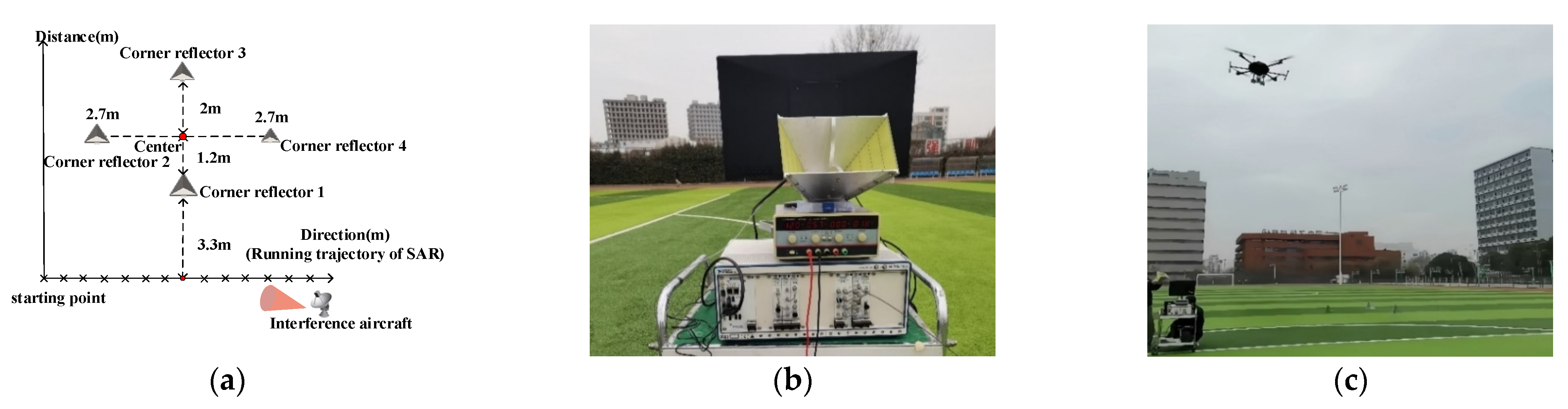
To study the effect of blanket jamming on the airborne SAR backward projection imaging results in the actual situation, the noise AM signal and the noise FM signal are transmitted by the jammer to simulate the jamming that may exist in the natural environment and record the corresponding experimental results. To obtain the experimental results under different noise levels, the transmitter power of the jammer is set to 10 dBm and 15 dBm, respectively, and the noise carrier is Gaussian white noise with a carrier frequency of 3.95 GHz. The experimental scenario after introducing the jammer is given in Figure 6.
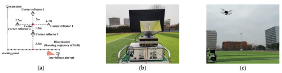
Figure 6.
Field experiment scene under jamming. (a) Experimental scenario design under jamming; (b) physical jamming aircraft; (c) airborne SAR detect target under jamming.
4.1. Noise Amplitude Modulation Jamming
Noise amplitude modulation (NAM) is one of the manifestations of a blanket jamming signal; a random signal formed after amplitude modulation of a carrier using noise. In the case of non-coherent jamming, the NAM signal model obtained using band-limited Gaussian white noise as the noise carrier is
In the above equation, and are constants and denote the amplitude and center frequency of the carrier frequency signal, respectively. The modulation noise is a generalized smooth random process with zero mean and variance . The phase is uniformly distributed on and is a random variable independent from . The total power of the noise modulation jamming is
where is referred to as the influential modulation factor, the total power of the AM signal is half of the carrier signal plus the modulating noise power.
The measured impact of NAM jamming on carrier-free ultra-wideband airborne SAR is shown in Figure 7.
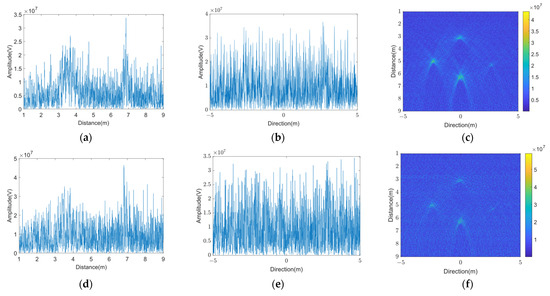
Figure 7.
The result under NAM jamming. (a) Distance result under 10 dBm NAM; (b) Direction result under 10 dBm NAM; (c) Result of BP algorithm under 10 dBm NAM; (d) distance result under 15 dBm NAM; (e) Direction result under 15 dBm NAM; (f) Result of BP algorithm under 15 dBm NAM.
The effect of noise amplitude modulation jamming on the original SAR image mainly originates from the interaction between the interfering signal and the target echo signal in the receiving and processing process. The amplitude modulation effect of the interfering signal changes the characteristics of the target echo signal, such as intensity, phase, and morphology, thus destroying the recognizability, clarity, and accuracy of the target in the image. The reasons why NAM jamming affects the quality of the original SAR image can be summarized as follows.
- The noise signal introduced by NAM jamming results in the intensity distortion of the target echo signal in the original SAR image. This intensity distortion may manifest as the amplitude modulation or attenuation of the target echo signal, causing the target’s brightness or reflectance characteristics to show abnormal variations in the image;
- The presence of NAM jamming reduces the contrast between the target and the background of the original SAR image, blurs the boundary between the target and the background, and makes the distinction between the target echo and the background noise decrease, thus reducing the clarity and discrimination of the image;
- NAM jamming causes phase distortion or amplitude changes in the target echo signal, leading to blurred target details in the original SAR image, resulting in unclear contours and fuzzy edges of the target and making it difficult to resolve the target morphology and structure.
4.2. Noise Frequency Modulation Jamming
Noise Frequency Modulation (NFM) jamming is easier to achieve wide bandwidth and large noise power than NAM jamming, so it is currently the main form of noise jamming. The signal model of Noise FM jamming is
where the modulating noise is a zero mean, generalized smooth random process and is uniformly distributed on and is a random variable independent of . is the amplitude of the NFM signal, is the center frequency of the interfering signal, and is the FM slope. The jamming bandwidth of the NFM signal is , which is independent of the noise bandwidth and is determined by and .
The measured impact of NFM jamming on carrier-free ultra-wideband airborne SAR is shown in Figure 8.
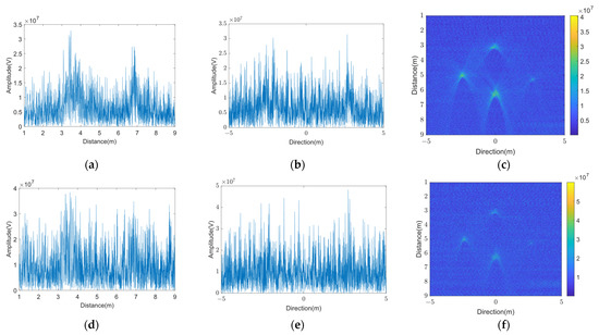
Figure 8.
The result under NFM jamming. (a) Distance result under 10 dBm NFM; (b) Direction result under 10 dBm NFM; (c) Result of BP algorithm under 10 dBm NFM; (d) Distance result under 15 dBm NFM; (e) Direction result under 15 dBm NFM; (f) Result of BP algorithm under 15 dBm NFM.
Streaks of non-uniform brightness appear on the SAR image. As the frequency of the NFM jamming signal is not smooth, it leads to a non-uniform distribution of energy in the SAR image; some areas may be subject to more substantial jamming and show higher energy levels, while other regions may have lower energy because the target echo signals are interfered with, so the places with higher frequencies on the SAR image are darker, i.e., the jamming is more substantial, which leads to a decrease in the visibility of the target in the image. The main reasons for the blurring of SAR images caused by NFM jamming are as follows:
- NFM jamming causes a frequency shift in the frequency of the original SAR signal, and the shift leads to a change in the spectral position of the echo signal, which prevents accurate integration of the target echo in the image and leads to blurred images;
- NFM jamming causes the phase distortion of the original SAR signal, and the phase distortion causes the phase of the echo signal to change, which affects the coherent superposition and synthesis of the echo from the same target, which in turn causes image blurring;
- When the jamming source modulates the power of the SAR signal, the NFM jamming will cause the intensity of the original SAR signal to change. This change in signal strength will lead to an uneven distribution of the energy of the target echo in the image, which in turn will affect the clarity and contrast of the picture.
4.3. Sinusoidal Frequency Modulation Jamming
Sinusoidal frequency modulation jamming (SFM) refers to the interference caused by an external signal that varies in frequency within a certain range and is in the form of a sinusoidal wave.
In Equation (12), represents the amplitude of the interference signal, denotes the frequency deviation, is the signal modulation frequency, stands for the signal carrier frequency, represents the signal phase, and represents the nth-order Bessel function. The measured impact of SFM jamming on carrier-free ultra-wideband airborne SAR is shown in Figure 9.
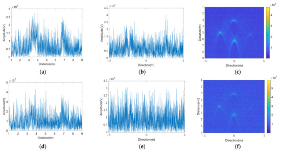
Figure 9.
The result under SFM jamming. (a) Distance result under 10 dBm SFM; (b) Direction result under 10 dBm SFM; (c) Result of BP algorithm under 10 dBm SFM; (d) Distance result under 15 dBm SFM; (e) Direction result under 15 dBm SFM; (f) Result of BP algorithm under 15 dBm SFM.
The blurring observed in the BP imaging results is attributed to the jamming of the SFM jamming signal on the signal, resulting in the following effects.
- When SFM jamming mixes with the signal during transmission, their frequency ranges may overlap, causing the jamming signal to overlap with the original signal in the frequency domain. This makes it difficult for the receiving end to accurately identify the original signal;
- During frequency modulation, changes in the signal’s frequency also result in changes in its amplitude, according to the properties of the Fourier transform. This can lead to distortion in the received signal.
5. Variational Mode Decomposition Algorithm for Anti-Jamming
5.1. Principles of the Variational Modal Decomposition Algorithm
Variational modal decomposition (VMD) mainly consists of two processes: constructing the variational problem and its solution. The VMD algorithm constructs the mathematical expression of the constrained variational problem based on the principles of classical Wiener filtering and Hilbert transform and iteratively solves it to obtain the center frequency and bandwidth.
In the VMD algorithm, the variational problem is the problem of finding the extremes of a generalized function, which is the objective function defined by the VMD-constrained variational model. By optimizing this objective function, the VMD algorithm can obtain more accurate and compact decomposition results.
Assuming that the input signal is a noise-laden SAR echo , the VMD algorithm decomposes the echo signal into IMF components with an AM-FM form . After applying the Hilbert transform to each element and obtaining its one-sided spectrum, the spectrum of each modal element can be shifted to its corresponding fundamental frequency by multiplying it with the phase factor
In Equation (13), , is the envelope function of , and is the instantaneous phase of .
Thus, the problem of finding the extremes of the generalized function is converted to the problem of minimizing the sum of the bandwidths of the center frequencies of these components. The constrained variational model of the VMD algorithm is as follows.
where and are the set of all modes and corresponding center frequencies, respectively.
To find the optimal solution, the quadratic penalty term and the Lagrange multiplier are introduced to convert the appeal-constrained problem into an unconstrained one. Among them, the weight value of the quadratic penalty term is inversely proportional to the noise signal, and the value of the quadratic penalty term has to converge to infinity in order to strictly guarantee the truth of the data in the assumption of noiselessness. On the other hand, the Lagrange multipliers are introduced to achieve the reconstruction constraints more strictly. Thus, the constraint problem becomes an augmented Lagrange function, as shown below.
The alternating direction multiplier method is used to solve this unconstrained problem, which is iteratively updated to obtain all the IMF components of the signal decomposition finally. The problem is converted to the frequency domain for processing using the Parseval–Fourier isometric transform and the results are obtained after iterations in the frequency domain.
The center frequency is updated adaptively and iteratively according to the following equation.
The convergence condition for stopping the update is
The complete steps of the VMD algorithm are as follows.
- (1)
- Initialize the values of , , , and . The decomposition modulus number is usually taken at 3~7;
- (2)
- Make and so that and are iteratively updated according to Equations (16) and (17);
- (3)
- When , the updated law of is expressed aswhere denotes the noise tolerance parameter, which is used in the VMD algorithm to control the degree to which the decomposition results are affected by noise.
- (4)
- Repeat steps 2 and 3 to make , , and adaptively updated, and stop the iteration when the parameters satisfy the convergence condition.
5.2. The Parameter Selection and Complexity Analysis of the VMD Algorithm
5.2.1. The Parameter Selection of the VMD Algorithm
- (1)
- Mode Number
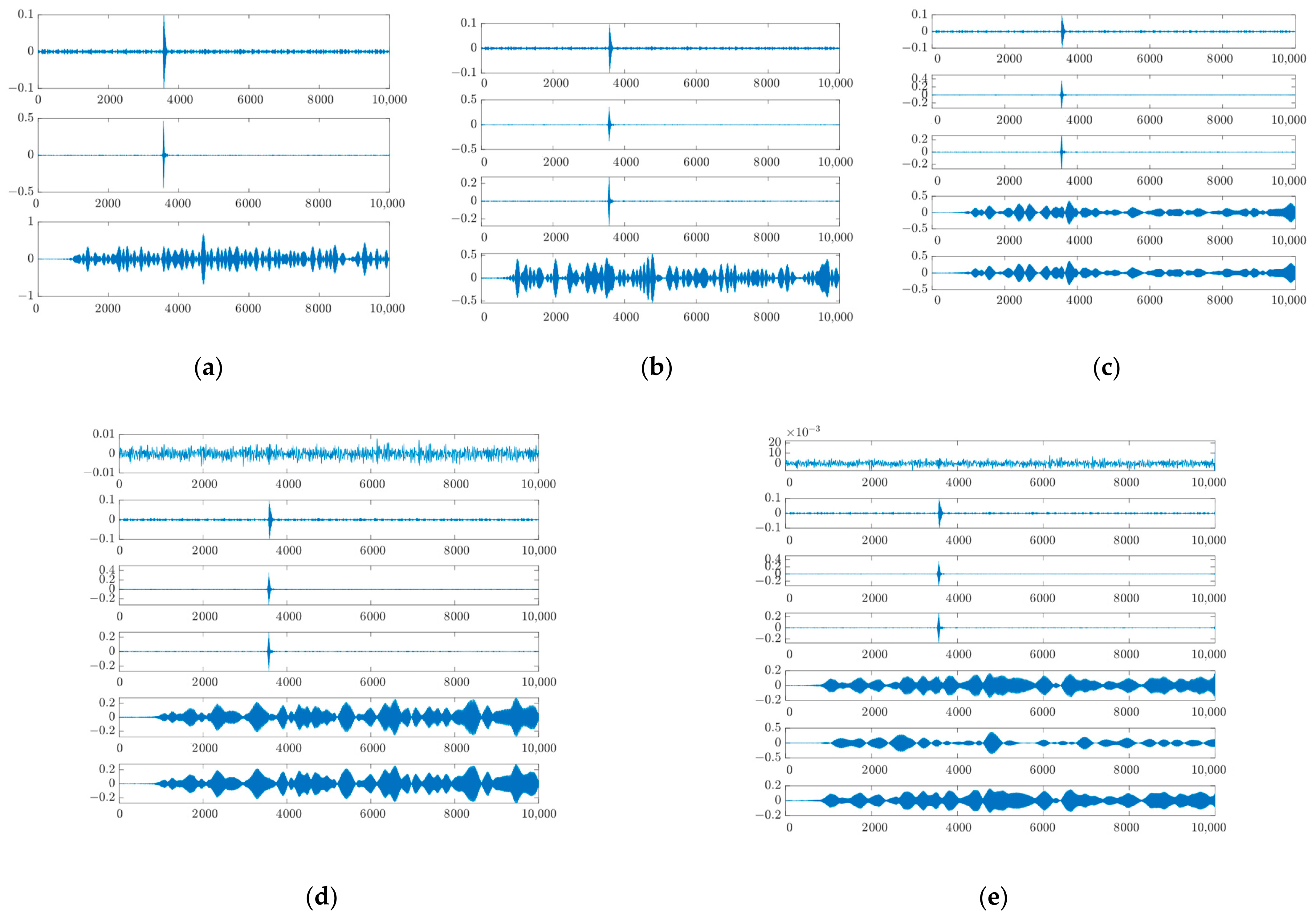
When using the VMD algorithm for modal decomposition, it is necessary to extract a predetermined number of modal components, denoted as . An appropriate value of allows for the correct partitioning of the signal’s frequency band and capture of IMF components at different frequencies. A higher number of modal components can more precisely describe the details of the signal but may also introduce overfitting or redundant information. Therefore, the determination of is crucial for the VMD algorithm. The decomposition modulus number is usually taken at 3~7. Using the fifth-order Gaussian pulse signal shown in Figure 1b, jamming conditions identical to the experimental setup were introduced. NAM jamming is taken as an example to select the value. Figure 10 depicts the reconstruction of signals under NAM, respectively, using the VMD algorithm with different values of .
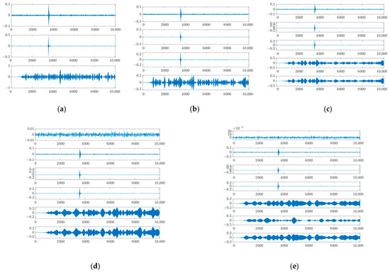
Figure 10.
IMF of VMD under NAM jamming. (a) IMF of K = 3; (b) IMF of K = 4; (c) IMF of K = 5; (d) IMF of K = 6; (e) IMF of K = 7.
After performing modal decomposition using the VMD algorithm, the required IMF components were selected for different numbers of decomposition modes. For , IMF1 and IMF2 components were chosen; for and , IMF1, IMF2, and IMF3 components were selected; and for and , IMF2, IMF3, and IMF4 components were chosen. Subsequently, the selected IMF signals were reconstructed, and the accuracy of the reconstructed signals was measured using the Pearson correlation coefficient.
In Equation (20), represents the variable and denotes the mean value of the variable. The larger the value of , the higher the signal correlation. When the decomposed modal number is , , , and , the correlation coefficients between the reconstructed signal of IMF components processed by the VMD algorithm and the original signal are shown in Table 1.

Table 1.
Pearson correlation coefficient of different mode numbers under NAM, NFM, and SFM.
In Table 1, it can be observed that when ranges from 3 to 7, the highest correlation between the reconstructed signal and the original signal is achieved when . Therefore, in this study, is chosen as the decomposed modal number.
- (2)
- Penalty coefficient
The penalty coefficient determines the bandwidth of the IMF components in the VMD algorithm. It is used to balance the data fitting and denoising effects in the optimization process. A larger value of leads to a smaller bandwidth of the IMF components, resulting in smoother decomposition results. Conversely, a smaller penalty coefficient yields larger bandwidths for the IMF components, potentially causing some components to include signals from other components. Therefore, a smaller regularization parameter tends to preserve more details and noise in the signal. The common range of this coefficient is between 1000 and 3000, with a default value of 2000 in this study.
- (3)
- The convergence condition
In two consecutive iterations, the optimization stops when the absolute average square improvement of the IMF component is less than . In this study, is set to , which allows for controlling the computational time and resources while ensuring accuracy.
5.2.2. The Complexity Analysis of the VMD Algorithm
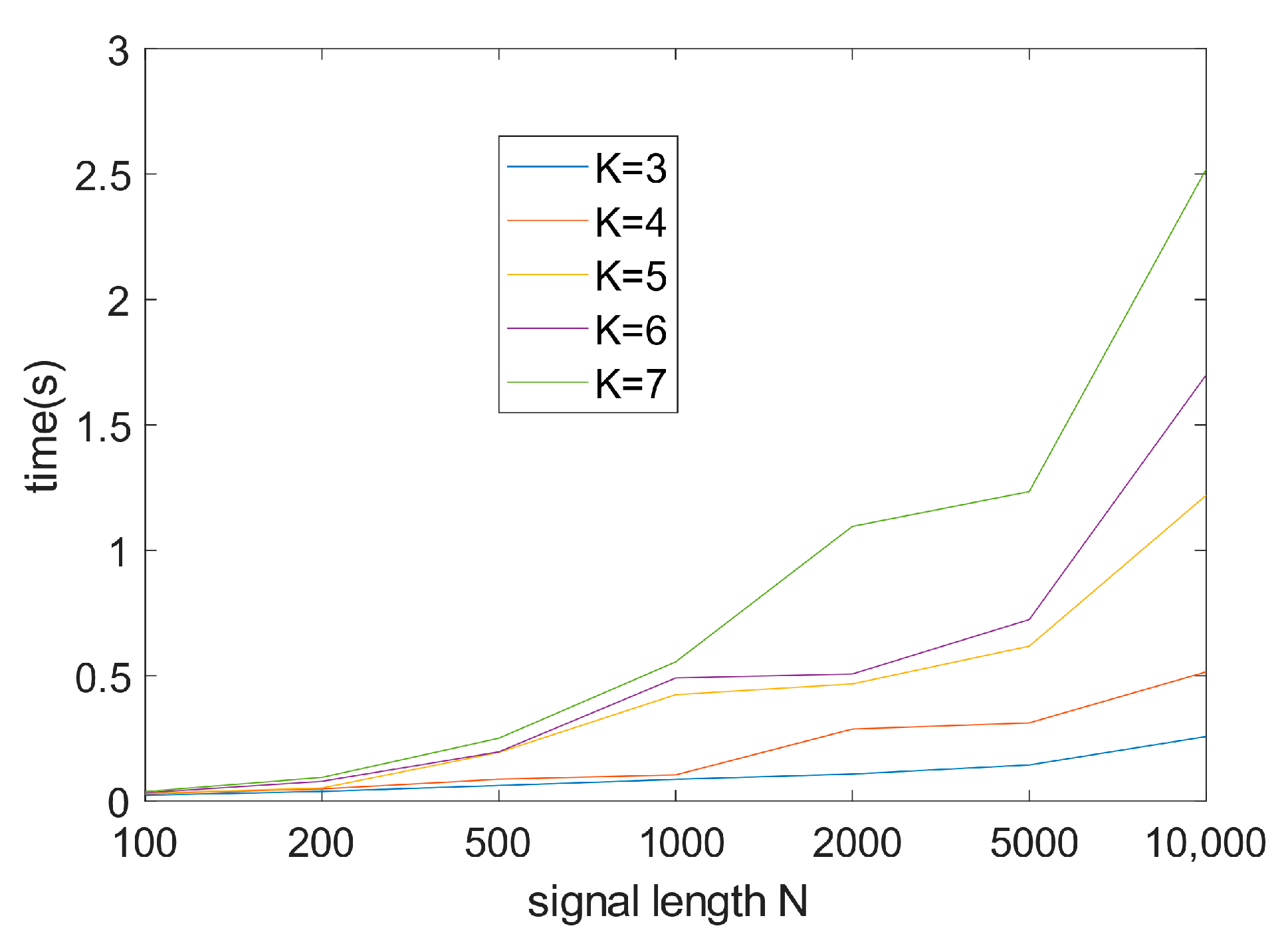
The time complexity of the VMD algorithm mainly depends on the number of iterations and the complexity of the inner loop in each iteration. The number of iterations of the VMD algorithm is determined by the convergence condition of the iteration, and the complexity of the inner loop depends on the signal length and the number of decomposition modes . Generally, as increases, the complexity of the inner loop will increase because more components need to be processed. Therefore, in this analysis, the algorithm complexity will be evaluated based on different values of and different lengths of signals as benchmarks.
The running time of the algorithm on a computer with an Intel i5-13400F CPU and dual-channel 2 × 16 GB memory is shown in Figure 11. When the signal length is relatively short, the algorithm’s running time is in milliseconds, and even when the signal length is 10,000, the running time of the algorithm is still in seconds. Based on the figure, it can be inferred that the time complexity of the algorithm is . In practical applications, it can efficiently and rapidly process signals for anti-interference, which validates the effectiveness and practicality of the algorithm.
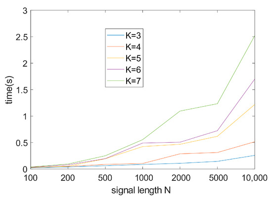
Figure 11.
Algorithm running time under different decomposition modes K and signal length N.
5.3. Experimental Verification of VMD Algorithm against Jamming
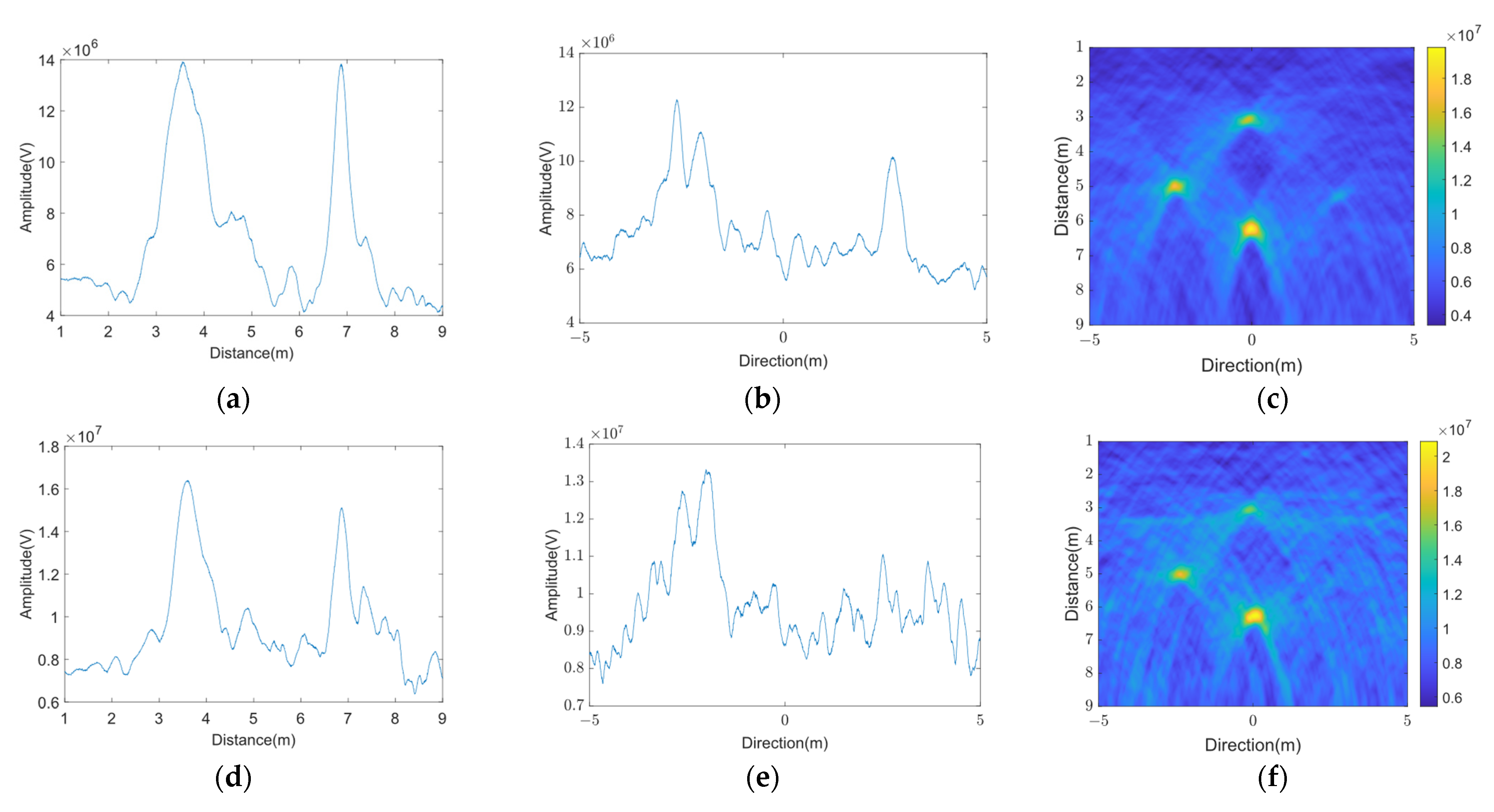
Figure 12 gives the imaging results of the EMD algorithm under NAM jamming. A comparison with Figure 7 can be found when the jamming power is 10 dBm after the EMD algorithm processes the target signal amplitude loss. Still, the processed signal retains the most significant features of the corner reflector echoes, the azimuthal direction of the surrounding clutter jamming is less, and the recovery of the image is better. However, as the jamming power increases, the reconstructed echo becomes more and more cluttered. At this time, the EMD algorithm cannot wholly separate the jamming from the signal, resulting in the IMF component used for reconstruction containing more noise components, the energy gap between the noise and the echo becoming smaller, and the noise occupying a more significant proportion of the image, resulting in the loss of the target’s information in imaging.

Figure 12.
The result of EMD under NAM jamming. (a) Distance result of EMD under 10 dBm NAM; (b) Direction result of EMD under 10 dBm NAM; (c) BP result of EMD algorithm under 10 dBm NAM; (d) Distance result of EMD under 15 dBm NAM; (e) Direction result of EMD under 15 dBm NAM; (f) BP result of EMD algorithm under 15 dBm NAM.
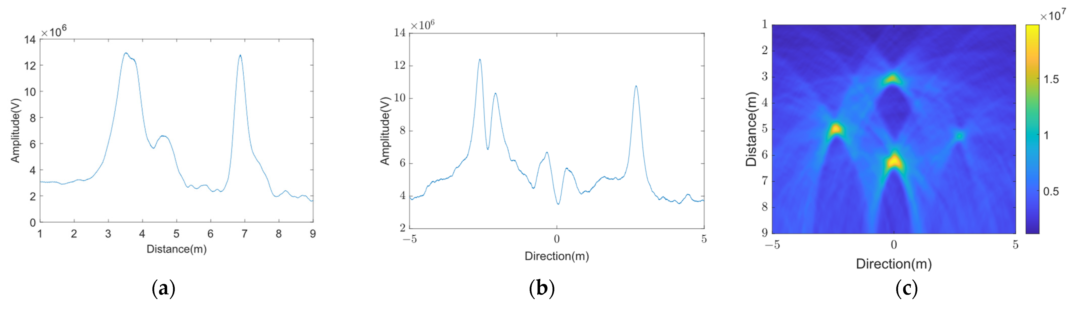
Figure 13 gives the imaging results of the VMD algorithm under noise amplitude modulation jamming. The figure shows that under the same jamming power, the VMD algorithm has better jamming suppression performance than the EMD algorithm; at this time, the azimuthal peak profile still retains the information of the central frequency band of the corner reflector, and the SAR image is still visible in the four corner reflectors. When the power of the jamming signal emitted by the jammer increases to a certain level, the reconstructed signal of the VMD algorithm contains more noise. Therefore, the position and details of the target cannot be recovered.
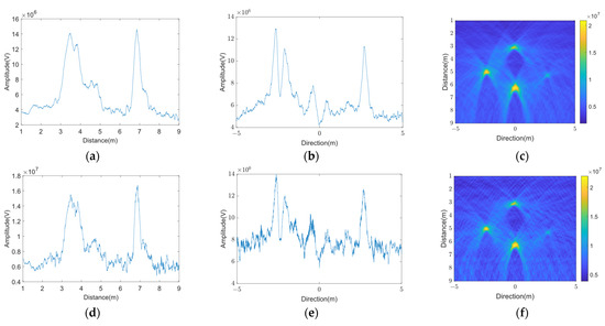
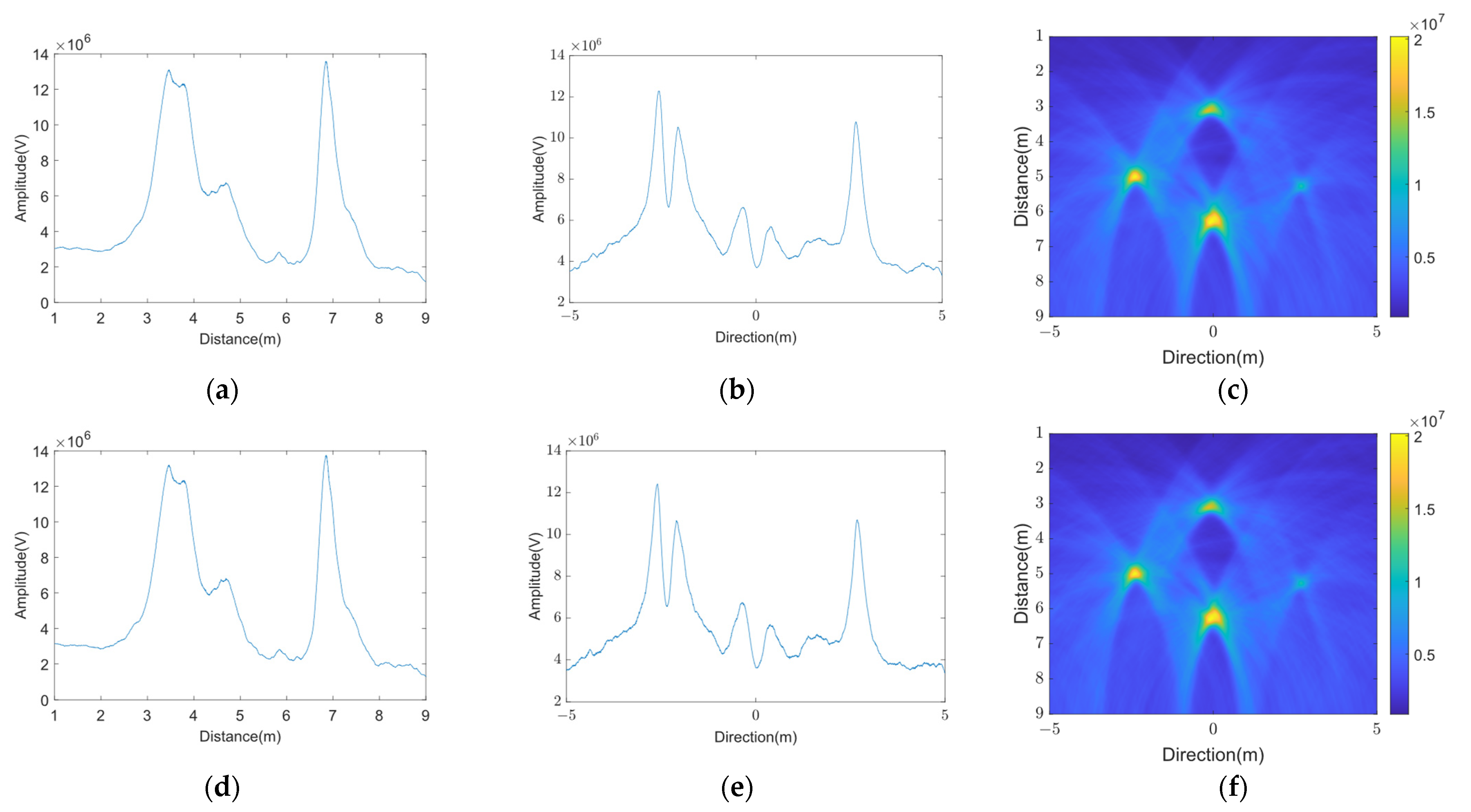
Figure 13.
The result of VMD under NAM jamming. (a) Distance result of VMD under 10 dBm NAM; (b) Direction result of VMD under 10 dBm NAM; (c) BP result of VMD algorithm under 10 dBm NAM; (d) Distance result of VMD under 15 dBm NAM; (e) Direction result of VMD under 15 dBm NAM; (f) BP result of VMD algorithm under 15 dBm NAM.
The experimental results of these two algorithms under NFM jamming are shown in Figure 14 and Figure 15. The EMD and VMD algorithms are better at dealing with NFM jamming. Since the EMD and VMD algorithms use only correlated modes for reconstruction, the recovered SAR image becomes smooth. Even though there is amplitude loss and clutter jamming in the reconstructed echo signal with increased jamming power, the data can still be used to image the experimental scene accurately. The VMD algorithm can recover the image better compared with the EMD algorithm.

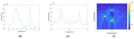
Figure 14.
The result of EMD under NFM jamming. (a) Distance result of EMD under 10 dBm NFM; (b) Direction result of EMD under 10 dBm NFM; (c) BP result of EMD algorithm under 10 dBm NFM; (d) Distance result of EMD under 15 dBm NFM; (e) Direction result of EMD under 15 dBm NFM; (f) BP result of EMD algorithm under 15 dBm NFM.

Figure 15.
The result of VMD under NFM jamming. (a) Distance result of VMD under 10 dBm NFM; (b) Direction result of VMD under 10 dBm NFM; (c) BP result of VMD algorithm under 10 dBm NFM; (d) Distance result of VMD under 15 dBm NFM; (e) Direction result of VMD under 15 dBm NFM; (f) BP result of VMD algorithm under 15 dBm NFM.
Figure 16 and Figure 17 present the anti-SFM jamming results of the EMD and VMD algorithms. It can be observed from the results that the VMD algorithm exhibits better resistance to SFM jamming compared to the EMD algorithm, leading to an improved restoration of the BP imaging results.

Figure 16.
The result of EMD under SFM jamming. (a) Distance result of EMD under 10 dBm SFM; (b) Direction result of EMD under 10 dBm SFM; (c) BP result of EMD algorithm under 10 dBm SFM; (d) Distance result of EMD under 15 dBm SFM; (e) Direction result of EMD under 15 dBm SFM; (f) BP result of EMD algorithm under 15 dBm SFM.
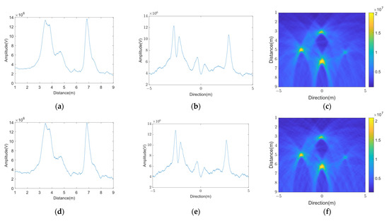
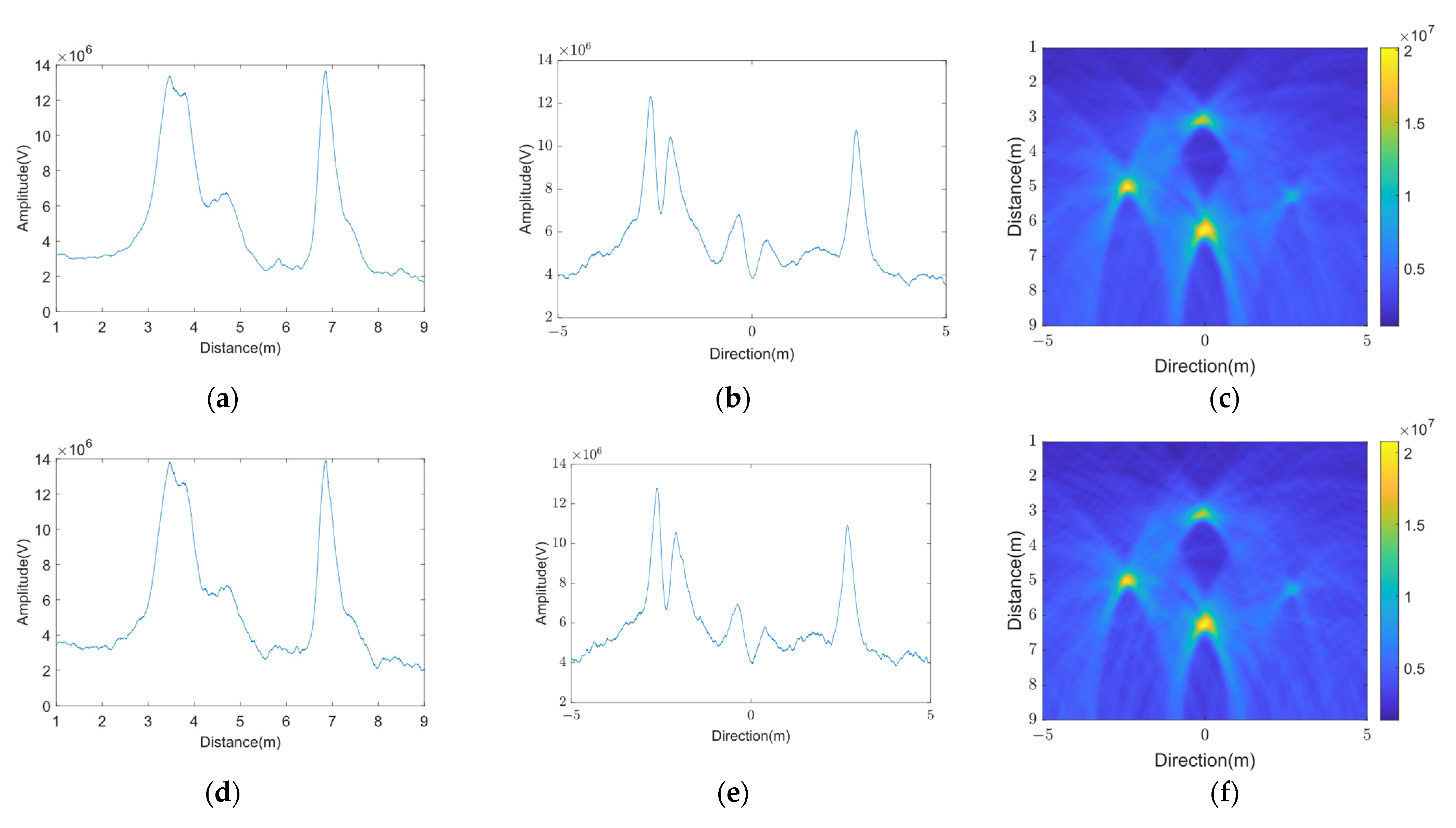
Figure 17.
The result of VMD under SFM jamming. (a) Distance result of VMD under 10 dBm SFM; (b) Direction result of VMD under 10 dBm SFM; (c) BP result of VMD algorithm under 10 dBm SFM; (d) Distance result of VMD under 15 dBm SFM; (e) Direction result of VMD under 15 dBm SFM; (f) BP result of VMD algorithm under 15 dBm SFM.
Through the above experimental results, the VMD and EMD algorithms show better results than the NAM jamming in suppressing NFM jamming and SFM jamming because both algorithms have strong frequency decomposition ability. The frequency characteristics of NFM jamming and SFM jamming change over time rather than the amplitude characteristics, so the VMD algorithm and the EMD algorithm can more accurately capture such frequency changes and separate them. Meanwhile, the NFM jamming and SFM jamming are usually non-smooth in time and have non-linear modulation characteristics. At the same time, the EMD algorithm and the VMD algorithm can better adapt to and extract this non-linear jamming, thus effectively reducing its impact on the image quality and improving the quality of the image restoration and the visibility of the target.
6. Algorithm Performance Comparison
To evaluate the anti-jamming effect of the deconvolution algorithm, its performance is compared with the EMD algorithm in terms of the Pearson correlation coefficient between the recovered signal and the original signal. Pearson correlation coefficient is a metric that reflects the degree of similarity between the estimated and original quantities and is calculated as shown in Equation (20).
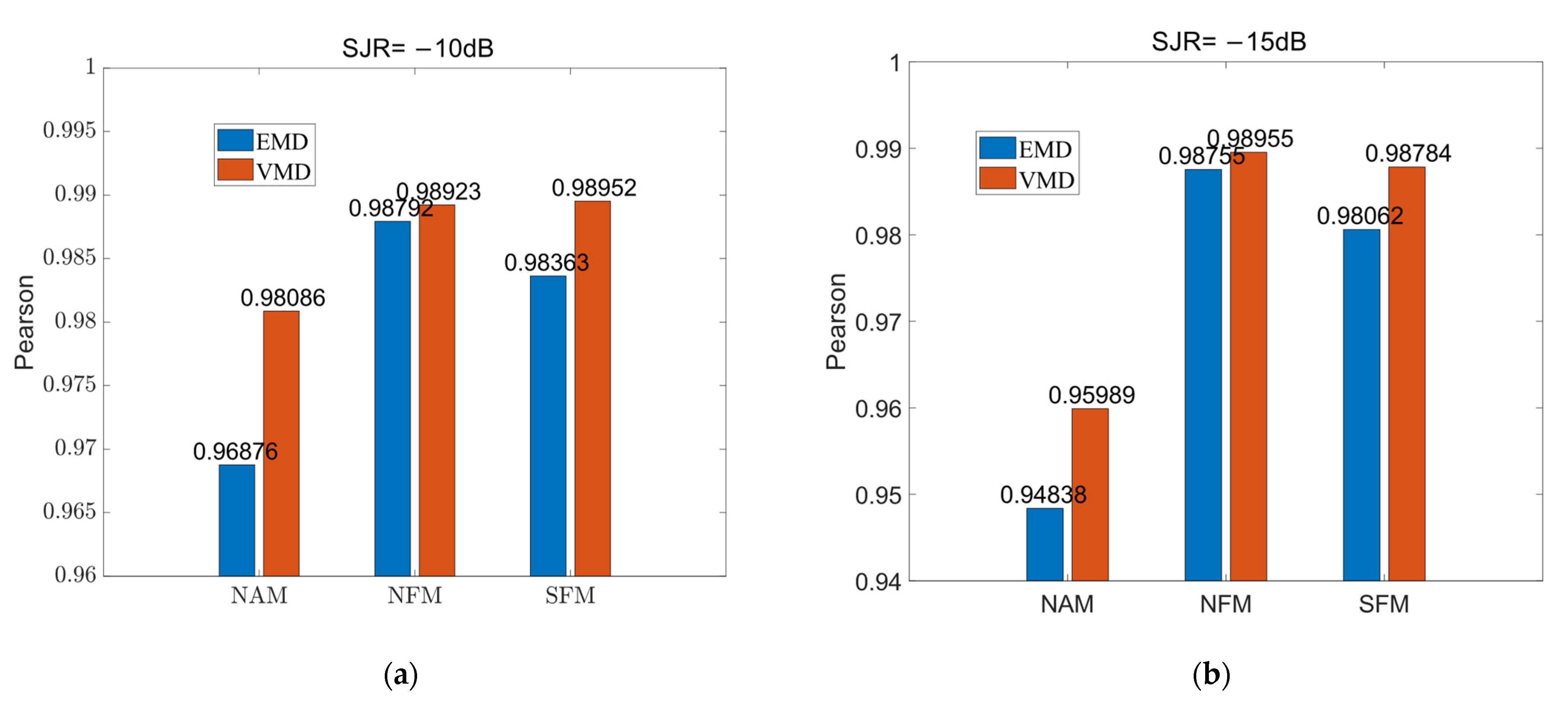
Figure 18 shows the correlation coefficient between the echo pulse of carrier-free ultra-wideband airborne SAR without jamming and the reconstructed signal using the VMD algorithm and EMD algorithm under NAM, NFM, and SFM.
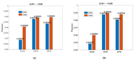
Figure 18.
Comparison between EMD and VMD. (a) Comparison under −10 dB; (b) Comparison under −15 dB.
Both the VMD algorithm and the EMD algorithm show the ability to suppress jamming. However, VMD has better anti-jamming ability, as can be seen from the bar graph, the signal reconstructed by the VMD algorithm has a higher Pearson correlation coefficient, so the VMD algorithm reconstructs the signal with higher accuracy and suppresses the blanket jamming better.
7. Conclusions
This study aims to investigate the effects of NAM jamming, NFM jamming, and SFM jamming on airborne SAR according to field experiments. The measured jamming data are taken as inputs, and the VMD algorithm is used to suppress this jamming, which is compared with the EMD, and a detailed comparative analysis is carried out. The results of the comparative analysis verify the effectiveness and efficiency of the VMD algorithm in suppressing NAM jamming, NFM jamming, and SFM jamming. Compared with the traditional EMD algorithm, the VMD algorithm shows better suppression effects and higher processing efficiency in processing jamming data. This study provides new ideas and solutions for the suppression methods of airborne synthetic aperture radar when subjected to different types of jamming, which is of great significance for improving the anti-jamming capability of radar systems. Meanwhile, this study also provides a valuable reference for future related research and promotes further in-depth discussion and development in anti-jamming technology.
Author Contributions
Conceptualization, Y.Y. and S.C.; methodology, Y.Y. and S.Z.; software, Y.Y. and C.Z.; validation, S.C. and W.T.; formal analysis, Y.Y. and W.T.; resources, Y.Y., S.Z. and S.C.; data curation, C.Z. and W.T.; writing—original draft preparation, Y.Y., C.Z. and S.C.; writing—review and editing, S.Z. and S.C.; visualization, Y.Y.; supervision, S.C.; project administration, S.Z.; funding acquisition, Y.Y. and S.C. All authors have read and agreed to the published version of the manuscript.
Funding
This work was supported in part by the National Natural Science Foundation of China (NSFC) under grant 62271261 and grant 62301252, the Natural Science Foundation of Jiangsu Province under grant BK20200075, and the Fundamental Research Funds for the Central Universities under grant 30922010717.
Data Availability Statement
The data presented in this study are available upon request from the corresponding author due to privacy restrictions.
Acknowledgments
The authors would like to thank the anonymous reviewers for their careful assessment of our work.
Conflicts of Interest
The authors declare no conflicts of interest.
References
- Liu, A.; Wang, F.; Xu, H. N-SAR: A New Multi-Channel Multi-Mode Polarimetric Airborne SAR. In Proceedings of the 2017 IEEE International Geoscience and Remote Sensing Symposium (IGARSS), Fort Worth, TX, USA, 23–28 July 2017; pp. 5394–5397. [Google Scholar]
- Li, C.; Yang, Y.; Yang, X.; Chu, D.; Cao, W. A Novel Multi-Scale Feature Map Fusion for Oil Spill Detection of SAR Remote Sensing. Remote Sens. 2024, 16, 1684. [Google Scholar] [CrossRef]
- Zhang, S.; Xu, L.; Long, R.; Chen, L.; Wang, S.; Ning, S. Quantitative Assessment and Impact Analysis of Land Surface Deformation in Wuxi Based on PS-InSAR and GARCH Model Remote Sensing. Remote Sens. 2024, 16, 1568. [Google Scholar] [CrossRef]
- Jin, S.; Bi, H.; Guo, Q.; Zhang, J.; Hong, W. Iterative Adaptive Based Multi-Polarimetric SAR Tomography of the Forested Areas Remote Sensing. Remote Sens. 2024, 16, 1605. [Google Scholar] [CrossRef]
- Cheng, S.; Zheng, H.; Yu, W.; Lv, Z.; Chen, Z.; Qiu, T. A Barrage Jamming Suppression Scheme for DBF-SAR System Based on Elevation Multichannel Cancellation. IEEE Geosci. Remote Sens. Lett. 2023, 20, 1–5. [Google Scholar] [CrossRef]
- Ammar, M.A.; Abdel-Latif, M.S.; Elgamel, S.A.; Azouz, A. Performance Enhancement of Convolution Noise Jamming Against SAR. In Proceedings of the 2019 36th National Radio Science Conference (NRSC), Port Said, Egypt, 16–18 April 2019; pp. 126–134. [Google Scholar]
- Chang, X.; Li, Y.; Zhao, Y.; Du, Y.; Liu, D.; Wan, J. A Scattered Wave Deceptive Jamming Method Based on Genetic Algorithm against Three Channel SAR GMTI. In Proceedings of the 2021 CIE International Conference on Radar (Radar), Haikou, Hainan, China, 15–19 December 2021; pp. 414–419. [Google Scholar]
- Zhao, P.; Dai, D.; Wu, H.; Pang, B. SAR Repeater Jamming Detection Method Based on Circle Frequency Filter. In Proceedings of the 2021 2nd International Conference on Electronics, Communications and Information Technology (CECIT), Sanya, China, 27–29 December 2021; pp. 1108–1112. [Google Scholar]
- Zhang, J.; Dai, D.; Xing, S.; Xiao, S.; Pang, B. A novel barrage repeater jamming against SAR-GMTI. In Proceedings of the 2016 10th European Conference on Antennas and Propagation (EuCAP), Davos, Switzerland, 10–15 April 2016; pp. 1–5. [Google Scholar]
- Li, J.; Jiang, B.; Liang, W.; Zhu, J.; Xiong, Y.; Tang, B. Swing Error Phase Modulation Jamming Method of Airborne SAR. In Proceedings of the 2019 International Conference on Communications, Information System and Computer Engineering (CISCE), Haikou, China, 5–7 July 2019; pp. 31–35. [Google Scholar]
- Huang, H.; Zhou, Y. An Inter/Intra-Pulse Partly Coherent Jamming Style against Synthetic Aperture Radar. In Proceedings of the 2012 IEEE 11th International Conference on Signal Processing, Beijing, China, 21–25 October 2012; Volume 3, pp. 2020–2022. [Google Scholar]
- Lee, Y.; Park, J.; Shin, W.; Lee, K.; Kang, H. A study on jamming performance evaluation of noise and deception jammer against SAR satellite. In Proceedings of the 2011 3rd International Asia-Pacific Conference on Synthetic Aperture Radar (APSAR), Seoul, Republic of Korea, 26–30 September 2011; pp. 1–3. [Google Scholar]
- Liu, Y.; Li, T.; Gu, Z. Research on SAR Active Deception Jamming Scenario Generation Technique. In Proceedings of the 2015 Fifth International Conference on Instrumentation and Measurement, Computer, Communication and Control (IMCCC), Qinhuangdao, China, 18–20 September 2015; pp. 152–156. [Google Scholar]
- Ji, P.; Xing, S. An Anti-Jamming Method Against SAR Stationary Deceptive Targets Based on DPCA Processing. In Proceedings of the 2019 IEEE 4th International Conference on Signal and Image Processing (ICSIP), Wuxi, China, 19–21 July 2019; pp. 264–268. [Google Scholar]
- Qiu, X.; Zhang, T.; Li, S.; Yuan, T.; Wang, F. SAR Anti-Jamming Technique Using Orthogonal LFM-PC Hybrid Modulated Signal. In Proceedings of the 2018 China International SAR Symposium (CISS), Shanghai, China, 10–12 October 2018; pp. 1–6. [Google Scholar]
- Sun, Z.; Zhu, Z. Anti-Jamming Method for SAR Using Joint Waveform Modulation and Azimuth Mismatched Filtering. IEEE Geosci. Remote Sens. Lett. 2023, 20, 1–5. [Google Scholar] [CrossRef]
- Yu, Q.; Zhu, D.; Wang, Y. Anti-jamming Method of MIMO-SAR with Dual Modulation of APC and OFDM. In Proceedings of the 2022 7th International Conference on Signal and Image Processing (ICSIP), Suzhou, China, 20–22 July 2022; pp. 701–706. [Google Scholar]
- Zhong, T. Sar Anti-Jamming Method Based on Optimization of Phase-Jittered LFM Signal. In Proceedings of the 2021 CIE International Conference on Radar (Radar), Haikou, China, 15–19 December 2021; pp. 796–799. [Google Scholar]
- Dragomiretskiy, K.; Zosso, D. Variational mode decomposition. IEEE Trans. Signal Process. 2013, 62, 531–544. [Google Scholar] [CrossRef]
- Zhao, S.; Chen, Y.; Ur Rehman, A.; Liang, F.; Wang, S.; Zhao, Y.; Deng, W.; Ma, Y.; Cheng, Y. The Inter-Turns Short Circuit Fault Detection Based on External Leakage Flux Sensing and VMD-HHT Analytical Method for DFIG. In Proceedings of the 2021 International Conference on Sensing, Measurement & Data Analytics in the era of Artificial Intelligence (ICSMD), Nanjing, China, 21–23 October 2021; pp. 1–5. [Google Scholar]
- Wu, Y.; Lin, Y.; Wang, J.; Qin, X.; Du, P.; Wang, F. Application of VMD in Fault Diagnosis for Rolling Bearing under Variable Speed Conditions. In Proceedings of the 2018 IEEE 3rd International Conference on Cloud Computing and Internet of Things (CCIOT), Dalian, China, 20–21 October 2018; pp. 275–278. [Google Scholar]
- Li, L. Research on Monthly Runoff Prediction based on VMD-BP model. In Proceedings of the 2023 5th International Conference on Frontiers Technology of Information and Computer (ICFTIC), Qingdao, China, 8–10 December 2023; pp. 740–744. [Google Scholar]
- McCorkle, J.W. Focusing of synthetic aperture ultra wideband data. In Proceedings of the IEEE International Conference on Systems Engineering, Dayton, OH, USA, 1–3 August 1993; pp. 1–5. [Google Scholar]


Disclaimer/Publisher’s Note: The statements, opinions and data contained in all publications are solely those of the individual author(s) and contributor(s) and not of MDPI and/or the editor(s). MDPI and/or the editor(s) disclaim responsibility for any injury to people or property resulting from any ideas, methods, instructions or products referred to in the content. |
© 2024 by the authors. Licensee MDPI, Basel, Switzerland. This article is an open access article distributed under the terms and conditions of the Creative Commons Attribution (CC BY) license (https://creativecommons.org/licenses/by/4.0/).