Article

Using Geostationary Satellite Observations to Improve the Monitoring of Vegetation Phenology

1
Key Laboratory of Agro-Ecological Processes in Subtropical Region, Institute of Subtropical Agriculture, Chinese Academy of Sciences, Changsha 410125, China
2
Huanjiang Observation and Research Station for Karst Eco-Systems, Huanjiang 547100, China
3
School of Remote Sensing and Information Engineering, Wuhan University, Wuhan 430072, China
4
Hubei Provincial Key Laboratory for Geographical Process Analysis and Simulation, Central China Normal University, Wuhan 430079, China
5
College of Urban and Environmental Sciences, Central China Normal University, Wuhan 430079, China
*
Author to whom correspondence should be addressed.
Remote Sens. 2024, 16(12), 2173; https://doi.org/10.3390/rs16122173
Submission received: 10 May 2024 / Revised: 8 June 2024 / Accepted: 11 June 2024 / Published: 15 June 2024
(This article belongs to the Section Remote Sensing in Agriculture and Vegetation)

Abstract

:
Geostationary satellite data enable frequent observations of the Earth’s surface, facilitating the rapid monitoring of land covers and changes. However, optical signals over vegetation, represented by the vegetation index (VI), exhibit an anisotropic effect due to the diurnal variation in the solar angle during data acquisition by geostationary satellites. This effect, typically characterized by the bi-directional reflectance distribution function (BRDF), can introduce uncertainties in vegetation monitoring and the estimation of phenological transition dates (PTDs). To address this, we investigated the diurnal variation in the normalized difference vegetation index (NDVI) with solar angles obtained from geostationary satellites since the image had fixed observation angles. By establishing a temporal conversion relationship between instantaneous NDVI and daily NDVI at the local solar noon (LSNVI), we successfully converted NDVIs obtained at any time during the day to LSNVI, increasing cloud-free observations of NDVI by 34%. Using different statistics of the time series vegetation index, including LSNVI, daily averaged NDVI (DAVI), and angular corrected NDVI (ACVI), we extracted PTD at five typical sites in China. The results showed a difference of up to 41.5 days in PTD estimation, with the highest accuracy achieved using LSNVI. The use of the proposed conversion approach, utilizing time series LSNVI, reduced the root mean square error (RMSE) of PTD estimation by 9 days compared with the use of actual LSNVI. In conclusion, this study highlights the importance of eliminating BRDF effects in geostationary satellite observations and demonstrates that the proposed angular normalization method can enhance the accuracy of time series NDVI in vegetation monitoring.

1. Introduction

Vegetation phenology refers to the regular variations in vegetation attributes influenced by factors such as precipitation and temperature [1]. This concept serves as a vital indicator of ecological shifts, highlighting the intricate connection between vegetation ecosystems and climate change [2]. Moreover, analyzing vegetation phenology can provide insights into changes in carbon storage [3], precipitation trends [4], and radiation balances [5]. Therefore, the accurate monitoring of vegetation fluctuations is essential for gaining a deeper understanding of worldwide environmental changes.
The utilization of remote sensing satellite data, with daily coverage, has significantly contributed to the global mapping of vegetation phenology [3,6]. These data encompass the Advanced Very-High-Resolution Radiometer (AVHRR) (AVHRR) [7], the Moderate Resolution Imaging Spectroradiometer (MODIS), and the Visible Infrared Imaging Radiometer Suite (VIIRS) [7,8,9,10]. These sensors mentioned above are carried on polar-orbiting satellites, which follow a set path and capture the Earth’s surface daily at a fixed time. Even though some sensors, like MODIS, can scan the Earth daily, the presence of frequent cloud cover limits their ability to collect reliable data and introduces uncertainty in the results of vegetation monitoring [11,12].
Geostationary satellites are essential components of the Earth Observation System (EOS). Positioned in a geostationary orbit (GEO), these modern satellites are equipped with advanced sensors that allow for detailed and accurate observations of the Earth comparable to sensors on polar-orbiting satellites [13,14]. Their ability to capture cloud-free images during daylight hours is facilitated by cloud movement, enabling multiple daily observations that increase the chances of obtaining clear images when compared to polar-orbiting satellites that provide only one observation at a fixed time each day [15,16]. For instance, in the northern USA, the Advanced Baseline Imager (ABI) on the Geostationary Operational Environmental Satellite 16 (GOES-16) provides about three times clearer observations than the Harmonized Landsat-8 and Sentinel-2 (HLS) dataset [17]. Similarly, a study by Zhao et al. compared the observations captured by the Advanced Himawari Imager (AHI) on Himawari-8 and MODIS in northern China, concluding the fact that the AHI captured 5.3 times more observations than MODIS [18].
Numerous endeavors have been dedicated to monitoring changes in vegetation through the utilization of geostationary satellites, leveraging their high time-frequency characteristics [19]. These endeavors have concentrated on a variety of vegetation types, including tropical broadleaf forests [20], temperate broadleaf forests [21,22], and shrublands [23]. The conclusions drawn from these studies suggest that the monitoring of surface vegetation phenology with geostationary satellites, either independently or in conjunction with other geostationary satellites, can yield comparable or even superior outcomes to those obtained using polar orbiting satellites. An analysis conducted by Yan [22] exhibited how precision in identifying the onset of the growing season for various vegetation types using AHI data was more than 40% higher than with MODIS data. Furthermore, research by Tian [17] uncovered the fact that the amalgamation of ABI and HLS data can reduce the margin of error in phenology extraction by almost 5 days, surpassing the utilization of ABI or HLS data individually.
The challenge lies in deriving a representative observation from multiple observations obtained from a geostationary satellite throughout the day. The variations in these observations are caused by the surface bidirectional reflectance distribution function (BRDF) effect [24,25]. Despite the fixed viewing angle per pixel provided by the geostationary satellite data, the changing solar angle during the time of observation poses a significant issue. For example, during the winter solstice over mid-latitude in the Northern Hemisphere (30°N), the solar zenith angle (SZA) changes by an average of 6.75° per hour. Furthermore, the vegetation index (VI), which is utilized for monitoring vegetation changes, such as the normalized difference vegetation index (NDVI), is greatly influenced by the BRDF effect [26,27]. The uncertainty of phenology monitoring can exceed 15 days due to the BRDF effect in the time series of NDVI data [25,28].
The BRDF effect of geostationary satellites has been documented by [24], and these frequent diurnal observations allow for the examination of the impact of solar angle variations on the observed NDVI. Although previous research has concentrated on the influence of viewing angles, which include the view zenith angle (VZA) and view azimuth angle (VAA) on the NDVI [27,29], the Walthall model, proposed in 1985 by Walthall et al., describes the changes in soybean canopy reflectance based on the VZA and VAA, without considering solar angle variations [30]. It was originally proposed in 1985 based on simulations of soybean canopy reflectance in the visible-near infrared band. This model focuses on the changes in canopy reflectance caused by variations in viewing angles but does not consider the changes in the solar angle, which limits the ability to predict reflectance at varying solar angles [31]. Therefore, a modification of the Walthall model is necessary to account for the solar angle correction in multiple observations within a day from geostationary satellites.
Two methodologies have been developed to mitigate the impact of surface BRDF and generate representative VI data from multiple diurnal observations provided by a geostationary satellite. One approach involves determining the 90th percentile of the angular-corrected VI (ACVI) values from cloud-free observations during a specific time window and treating it as the accurate value for the day [17,22]. An alternative method consists of averaging the VI values derived from all cloud-free observations on a given day and utilizing the daily average VI (DAVI) to reconstruct the time series VI curve [18]. However, consistent data are essential for vegetation phenology monitoring to avoid uncertainties from anomalous fluctuations in time series VI [1]. These two methods are based on daily VI values obtained through statistical means, which do not align with the observation time, thus posing challenges in ensuring the physical consistency of the time series VI.
Therefore, in this study, we employed the SZA and solar azimuth angle (SAA) as the independent variables to model the variations in NDVI, enabling the inversion of NDVI for each pixel at local solar noon. The purpose of this study is to propose a method for eliminating the BRDF effect in the multiple observations from geostationary satellites throughout the day and reconstruct a highly consistent time series NDVI curve to identify typical vegetation transition dates. This method was applied to the data from the Chinese geostationary satellite Fengyun-4 (FY-4) Advanced Geosynchronous Radiation Imager (AGRI), and it involved (1) using cloud-free observations within a specific time window to fit the NDVI obtained under cloud cover, thereby alleviating the influence of clouds; (2) retrieving the local solar noon NDVI (LSNVI) from multiple NDVIs of geostationary satellites as a representative vegetation index for the day during vegetation monitoring; and (3) exploring the variability of different methods when constructing time series vegetation indices for phenology extraction based on geostationary satellite data.

2. Data and Methods

2.1. Data

2.1.1. FY-4 ARGI Images

The FY-4A is a new-generation geostationary satellite launched by China on 11 December 2016, which is positioned at a longitude of 104.7°E [32]. Equipped with 14 spectral bands, the FY-4 AGRI captures a full-disk scan every 15 min, providing resolutions of 1 km, 2 km, and 4 km for the visible, near-infrared, and infrared bands, respectively. Access to FY-4A data has been available since 12 March 2018 from the Fengyun Satellite Data Center (http://data.nsmc.org.cn, accessed on 1 May 2024). This study utilized the full-disk surface reflectance data obtained after the rapid atmospheric correction of FY-4 AGRI, specifically focusing on the 1 km spatial resolution spectral surface reflectance data for AGRI band 2 (centered at 0.65 μm), band 3 (centered at 0.83 μm), and band 5 (centered at 1.61 μm). The data collection period ranged from 1 June 2018 to 31 December 2021 during the Universal Time Coordinated (UTC) from 00:00 am to 9:00 am, resulting in a total of 16 fixed observations at a specified time per day.

2.1.2. In Situ Measurements
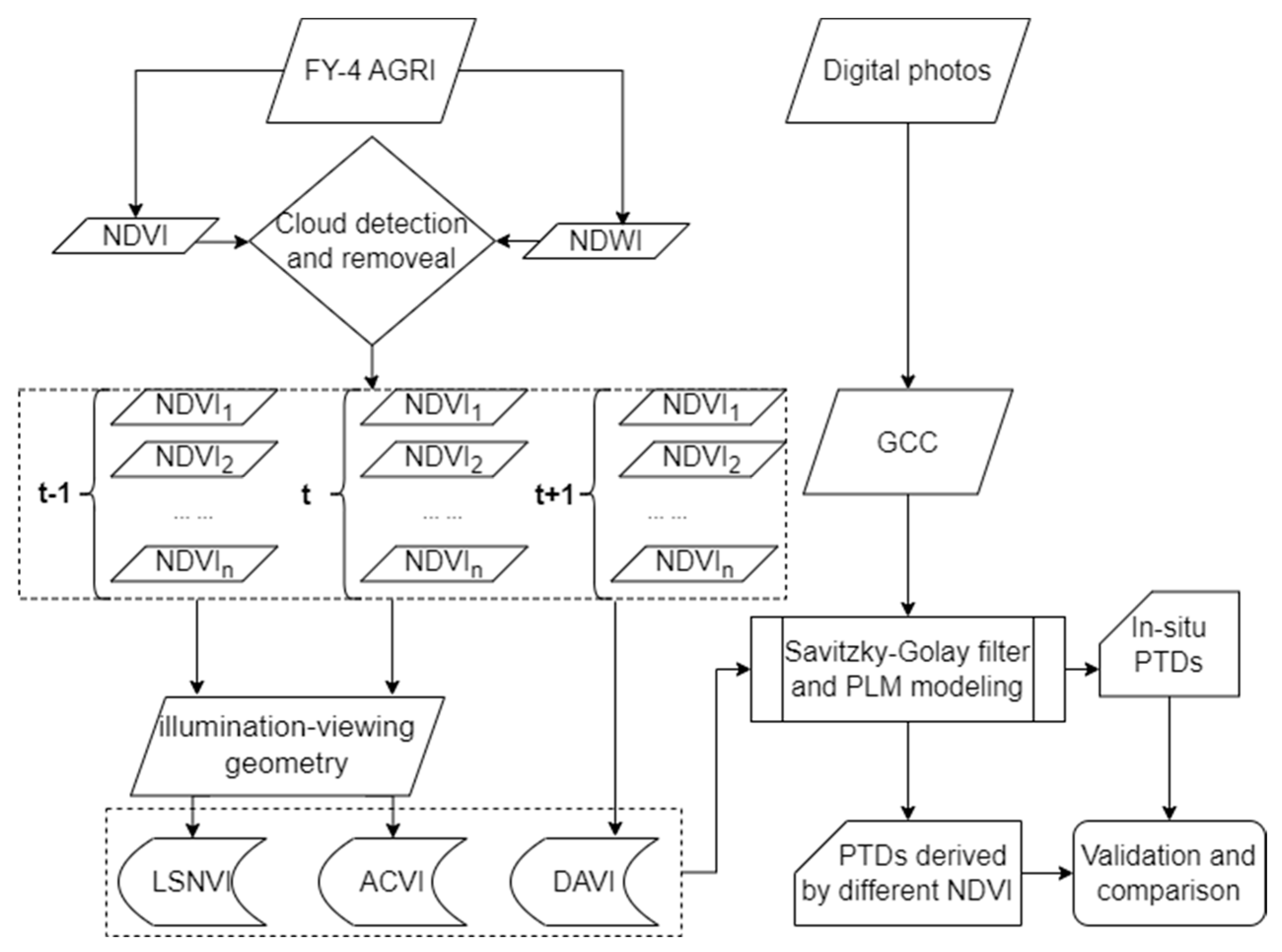
Near-surface digital repeat photography is an important data source for the validation of phenological information obtained from satellite data [33,34]. In this study, the in situ measurements of five ground sites with different climate and vegetation types in China were obtained. The data from these three sites, Arou, Daman, and Liancheng, were collected from the National Qinghai–Tibetan Plateau Scientific Data Center (TPDC) (https://data.tpdc.ac.cn, accessed on 1 May 2024) [35], while the data from Jurong and Shangqiu were obtained from the PhenoCam network (https://phenocam.nau.edu, accessed on 1 May 2024). Comprehensive details about the ground sites can be found in Table 1.
These sites were equipped with digital cameras that captured images every thirty minutes. Digital photographs were used to provide in situ measurements to evaluate satellite-derived vegetation phenological information. Data preprocessing was performed to select high-quality daily photos, where the region of interest (ROI) in the photos was identified, and the green chromatic coordinate (GCC) was calculated. Subsequently, GCC curves representing the time series data for each site were generated.
GCC = G/(R + G + B),
where R, G, and B represent the digital number from the red, green, and blue channels of the digital photos, respectively.

2.2. Methods

The entire structure of vegetation monitoring and the comparison of the VI constructing methods process consists of four main steps. Firstly, we identified cloudy observations in the multiple daily observations from geostationary satellites. Secondly, we established a time window centered on the target day of the year (DOY) and utilized the cloud-free observations within the window to estimate the LSNVI on the target DOY. Thirdly, we reconstructed the ACVI and DAVI on the target DOY using cloud-free observations within the time window. Finally, the piecewise logistic model (PLM) proposed by Zhang [8] was employed to detect the phenology transition date (PTD) from the time series LSNVI, ACVI, and DAVI curves, and the accuracy of the extracted PTD based on three different time series VIs was compared. The workflow is illustrated below (Figure 1), and each step is detailed in the subsequent sections.

2.2.1. Cloud-Free NDVI Construction

NDVI serves as a crucial indicator for describing alterations in vegetation dynamics and has been extensively employed in monitoring the phenological dynamics of various vegetation types. In this study, we computed NDVI using FY-4 surface reflectance data.
N D V I = ρ N I R ρ r e d ρ N I R + ρ r e d ,
where ρNIR and ρred are the spectral reflectance of near-infrared (NIR) and red bands. To obtain the cloud-free NDVI, we calculated the normalized difference water index (NDWI) to filter out the NDVI obtained from observations of clouds in a day.
N D W I = ρ N I R ρ S W I R ρ N I R + ρ S W I R ,
where ρSWIR is the spectral reflectance in the short-wave near infrared (SWIR) band. In Equations (2) and (3), the red, NIR, and SWIR bands correspond to bands 2, 3, and 5 of AGRI, respectively. The NDVIs during the day were removed if NDWI > NDVI [17], and the cloud-free NDVI was derived.

2.2.2. Retrieving the NDVI at Local Solar Noon

To ensure the consistency of NDVI values from day to day, we employed LSNVI as a representation of the true NDVI values for a single day. The geostationary satellite orbit remains fixed relative to the Earth, resulting in consistent values for the VZA and VAA for each pixel in the image. We calculated the VZA and VAA for each pixel in the full disk of FY-4 AGRI data (Figure 2). Thus, the differences in multiple NDVIs obtained from observations of each pixel during the day are mainly due to variations in solar angles. An assumption was made that the vegetation phenology remains constant throughout the day. Therefore, any variations observed in the multiple cloud-free NDVIs within a day can be attributed to changes in the solar angle, which include SZA and SAA [18,25,36].
To investigate how the NDVI changes with the SZA and SAA throughout the day, we first calculated the SZA and SAA of multiple observations provided by FY-4 AGRI on a certain day. Then, we used the PROSAIL model [37] to simulate the canopy NDVI under various leaf area index (LAI) conditions; the input of the PROSAIL model is listed in Table 2. Finally, we collected all the cloud-free FY-4 AGRI observations taken at a ground station throughout the day and calculated the NDVI at different times.
Inspired by the Walthall model [30], we made modifications to account for the fixed viewing angle of a geostationary satellite and the varying solar angle. We adjusted the viewing angle (VZA and VAA) in the model to be the solar angle (SZA and SAA) and established a relationship between the solar angle and canopy NDVI [38].
N D V I = a θ s 2 + b θ s cos ( φ s φ v ) + c ,
where a, b, and c are the coefficients, θs is the SZA, and φs and φv are the SAA and VAA, respectively. To ensure the fit of the NDVI at local solar noon, we first needed to determine the coefficients a, b, and c based on multiple observations. To ensure the stability of the obtained coefficients, we set a time window of three days, and all cloud-free observations during the window period were input as samples to fit the coefficients into the model. A threshold of 15 observations was adapted to ensure sufficient data availability for the valid statistical inversion for the estimation of the coefficients. If the number of valid observations within the time window was below the threshold, no valid observations were considered for that day. Then, we calculated the SZA of a pixel at local solar noon using the latitude of the pixel and the latitude of the direct solar point, which can be determined from the date. At local solar noon, the SAA of a pixel is defined as 180°, and the VZA and VAA are fixed. Once all the variables on the right side of the equation were determined, we could estimate the NDVI at local solar noon.

2.2.3. Construction of Different Time Series VI Curves

Here, we calculated two measurements from geostationary satellite data, DAVI and ACVI, to make a comparison of the time series NDVI curve formed by LSNVI. The DAVI was calculated by removing the cloudy observations and taking the daily average NDVI under cloud-free observations as the NDVI of that day [18]. The ACVI was calculated by correcting all the cloud-free NDVI in a day to a certain fixed illumination viewing geometries first, and the angular corrected values using Equation (5). Then, the 90% quantile of the ACVI value within a certain time window was chosen as the ACVI of the center day of the time window [22].
A C V I ( θ r e f , δ r e f , ϕ r e f ) = N D V I ( θ t , δ t , ϕ t ) ( 1 + C 0 S r e f + C 1 R r e f ) ( 1 + C 0 S t + C 1 R t ) ,
where ACVI(θref, δref, ϕref) is the NDVI under a fixed illumination viewing geometry (θref = 45°, δref = 45°, ϕref = 45°)); θ is SZA; δ is VZA; ϕ is the relative azimuth angle (RAA); NDVI(θt, δt, ϕt) is the original NDVI obtained under the illumination viewing geometry at time t; S and R are the kernel functions that model the variations in NDVI due to the differences in illumination viewing geometries; and C0 and C1 are kernel weights that were determined as −0.08 and 0.02 based on the previous study [39].

2.2.4. Phenological Information Extraction and Validation

First, we employed the Savitzky–Golay (S-G) filter [40] to smooth the irregular NDVI and GCC values. Subsequently, we utilized double logistic curves to fit the smoothed NDVI and GCC time series for temporal trajectory reconstruction. This involved the application of the PLM algorithm proposed by Zhang [8] to fit the smoothed time series of NDVI and GCC. By computing the rate of change in curvature from the reconstructed temporal trajectory, the local extreme values of this rate represented the four phenological transition dates (PTDs), namely, (1) greenup, marking the onset of photosynthesis; (2) maturity, the date of the maximum green leaf area; (3) senescence, the date of rapid decrease in photosynthetic activity and green leaf area; and (4) dormancy, the date when physical activity nears zero [8]. Subsequently, the PLM was utilized to detect the four PTDs from the time series LSNVI, ACVI, and DAVI curves, respectively. Furthermore, the accuracy of the phenological extraction results was evaluated using two metrics, namely the mean absolute error (MAE) and the root mean square error (RMSE), which were further utilized to compare the three different NDVI reconstruction methods.
M A E = 1 m i = 1 m y i x i ,
R M S E = i = 1 m ( y i x i ) 2 m
where x and y are the PTDs derived by the GCC and NDVI time series, respectively; i is the index; and m is the number of PTDs.

3. Results

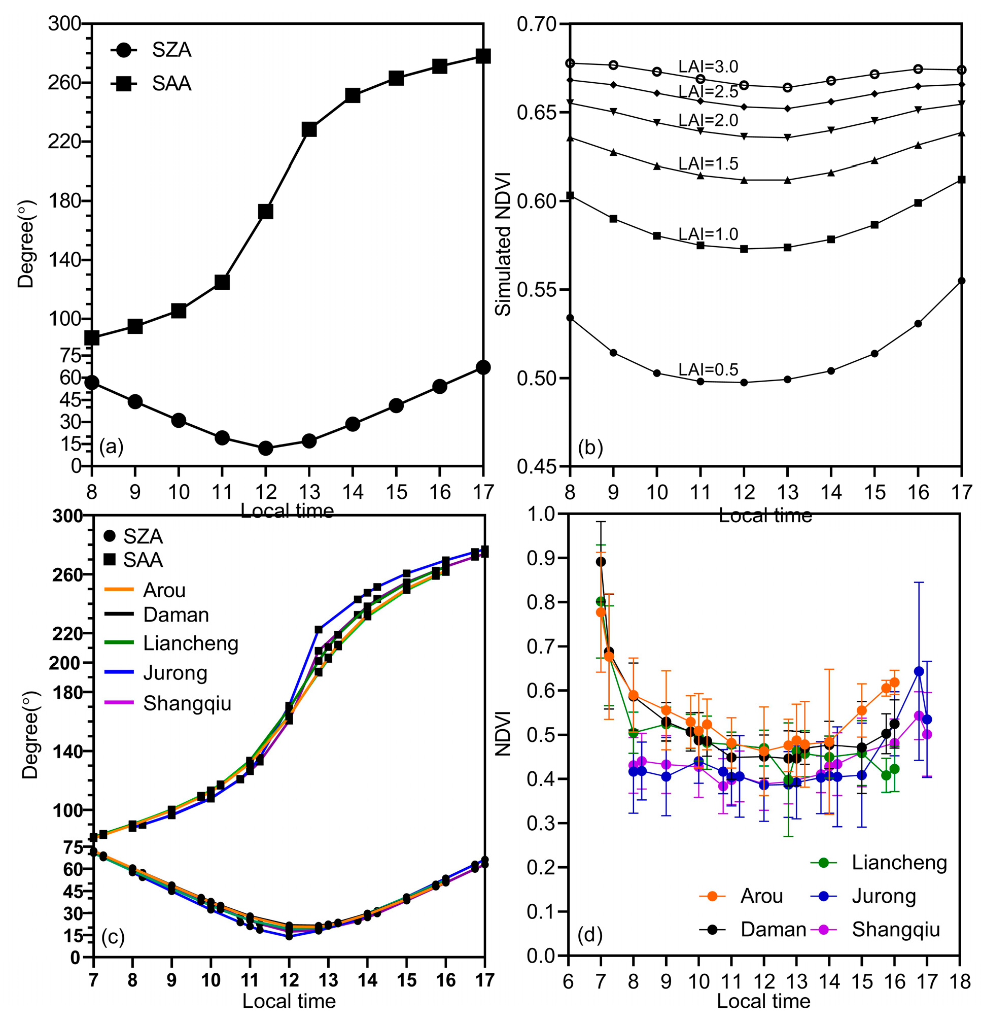
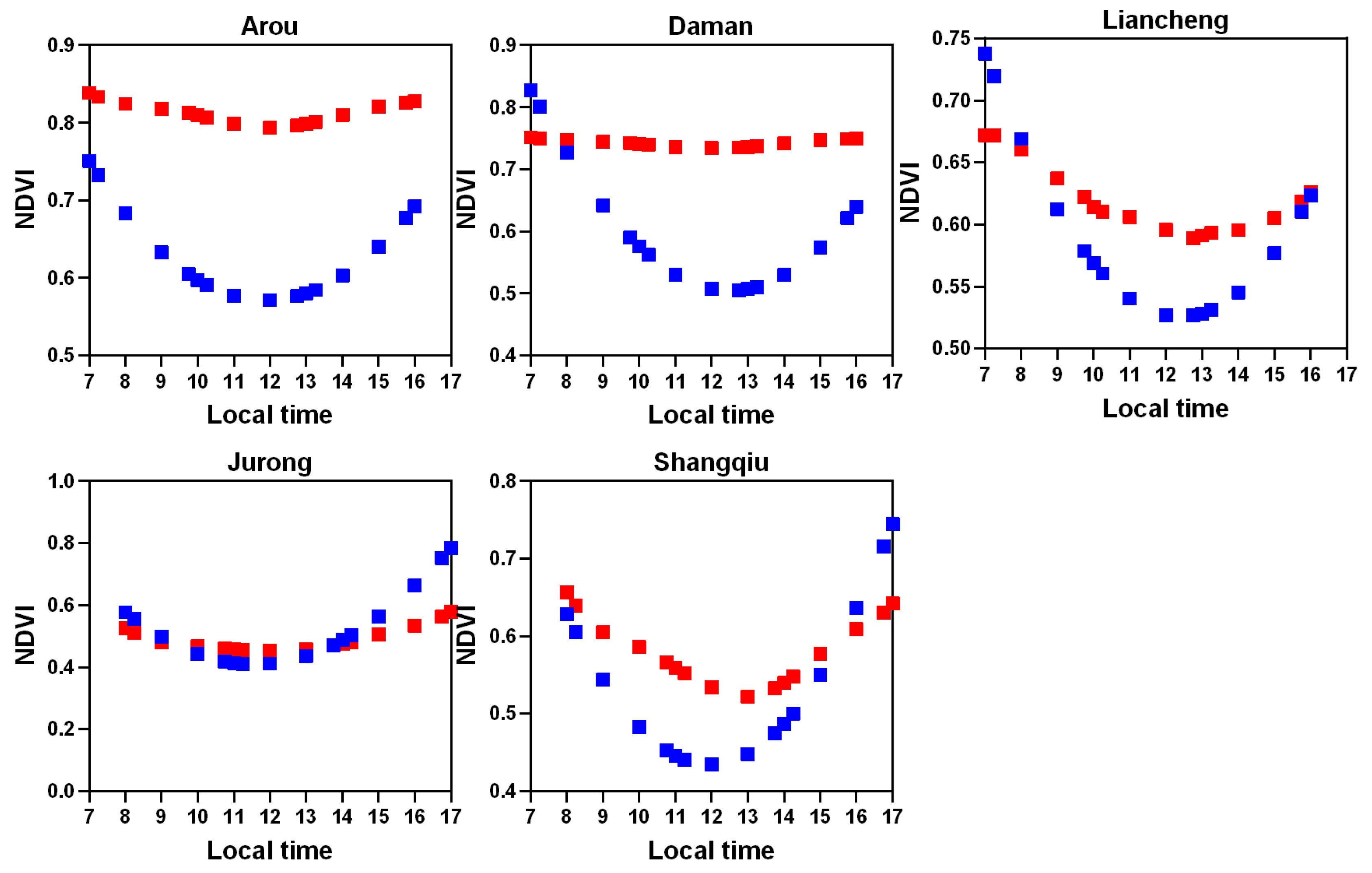
3.1. The Diurnal Variation in the FY-4 NDVI

The calculated and actual solar angle (SZA and SAA) shows the same diurnal variation; it revealed that the SZA reaches its minimum at local solar noon and its maximum in the early morning or late afternoon, and its variation is symmetrically distributed with the local solar noon (Figure 3a,c). The SAA, on the other hand, is monotonically distributed and remains constant at 180° at local solar noon. The estimation of canopy NDVI showed that the shape of NDVI roughly follows a bowl shape throughout the day. The trend of NDVI changes in correlation with the variation in SZA; thus, a smaller SZA (i.e., close to local solar noon) results in a smaller NDVI. The NDVI in the early morning or late afternoon was 11.57% higher than that at local solar noon (Figure 3b), and this difference decreased with the increase in LAI. The shape of the diurnal variation in NDVI was also evidenced by the true observations of the FY-4 AGRI. As shown in Figure 3d, the 16-day average NDVI at the Liancheng site in the early morning or late afternoon was 91.04% compared to that at the local solar noon, and the smallest difference in the Arou site also reached 35.80%.

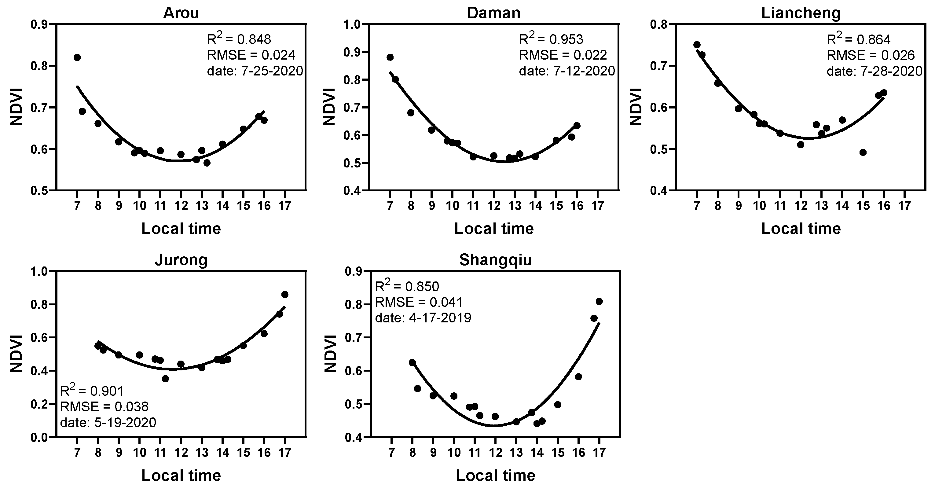
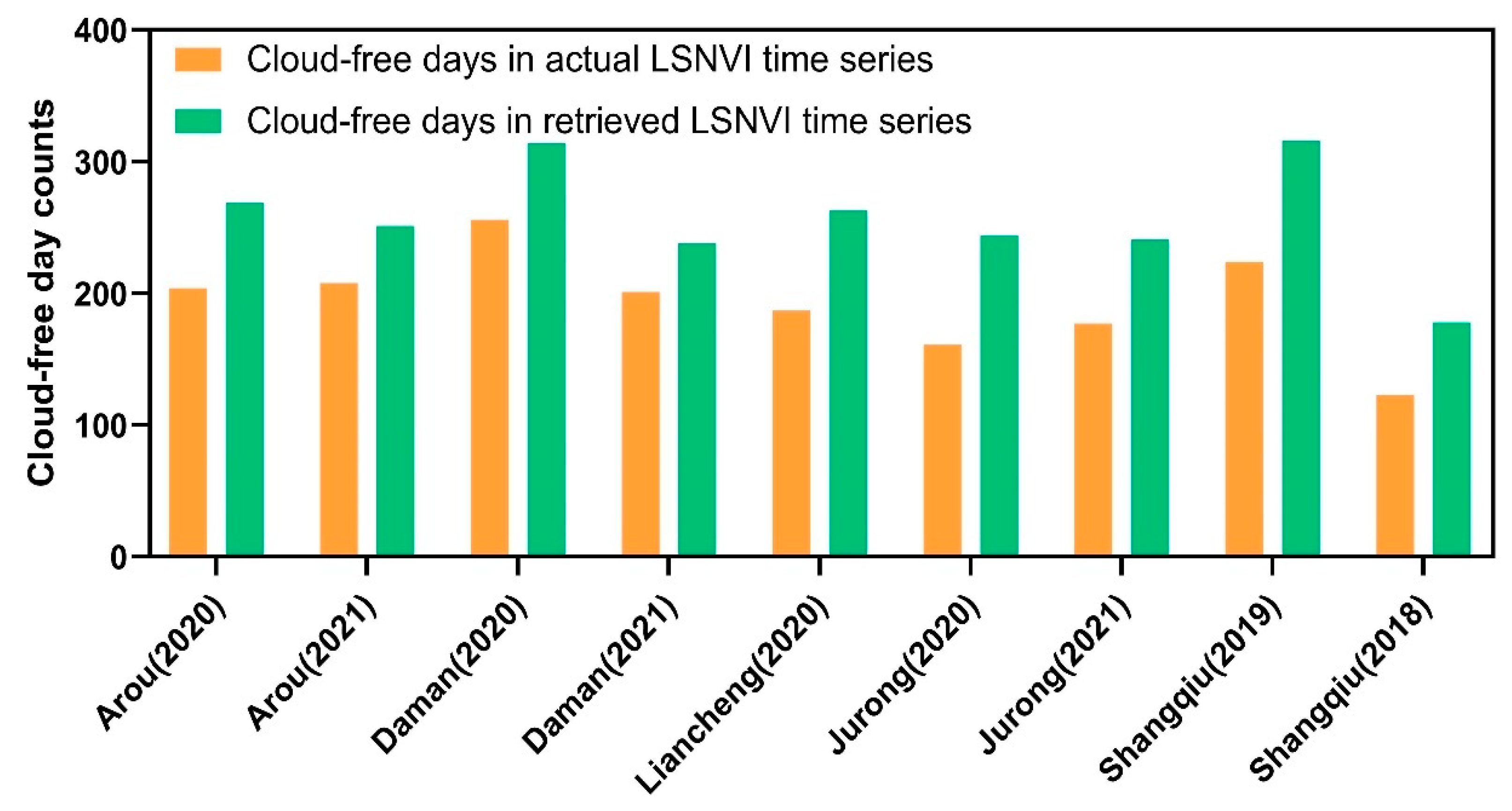
3.2. Retrieval Results of Local Solar Noon NDVI (LSNVI)

The NDVI fitted results for the ground sites, as shown in Figure 4, indicate that the model performed well across all sites, with an R2 value of over 0.84 and an RMSE value below 0.05. The results at the Daman site exhibited the best fit, with an R2 value exceeding 0.84 and an RMSE value below 0.05. Conversely, the Shangqiu and Jurong sites showed the poorest fit, with relatively high RMSE values.
The accuracy of the LSNVI retrieval model was validated by estimating the LSNVI for each day of the given year at the five stations. These values were then compared with the actual LSNVI after excluding any cloudy observations. The results are presented in Figure 5. From the validation results, it was observed that the R2 values for all sites ranged from 0.753 to 0.951 for the corresponding years. In 2019, the Jurong site had the lowest R2 value, while the Daman site had the highest R2 values in both 2020 and 2021. For all years, the NDVI values at all sites were negative and remained relatively stable at around −0.02. In terms of bias, the Jurong site had the lowest value in 2019 (−0.017), while the Daman site had the highest values in both 2020 and 2021 (−0.028). The RMSEs varied across the different sites and years, ranging from 0.038 to 0.053. The Daman site had the lowest RMSE value (0.038) in both 2020 and 2021, while the largest RMSE value (0.053) was recorded in 2021 at Liancheng.

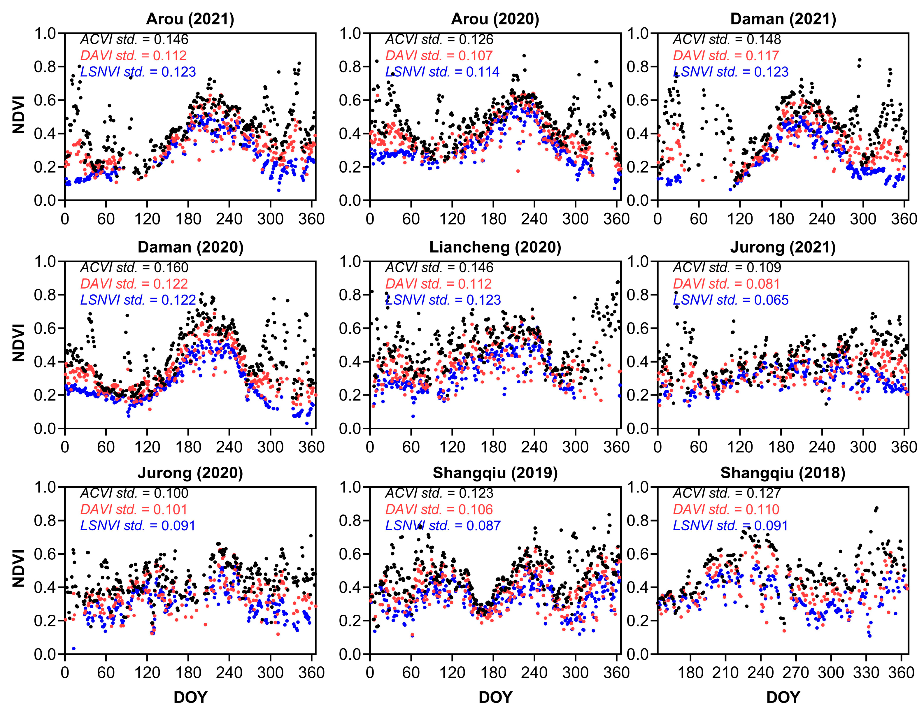
3.3. The Seasonal Variation in Different VIs

The temporal VI curves were reconstructed using three different time series VIs displayed in Figure 5. Upon the analysis of Figure 6, it is evident that the daily LSNVI has relatively low values compared with ACVI and DAVI. To assess the stability of the reconstructed time series of NDVI using different methods, we computed the standard deviation of the NDVI values. The standard deviation of the time series LSNVI also had relatively low values compared with ACVI and DAVI. The ACVI yields the highest standard deviation of the time series data for different years and locations, while the DAVI produces the second-highest standard deviation. Upon the quantitative evaluation of the standard deviation of the time series of NDVI reconstructed using different methods, we found that the change in the intra-annual pattern of NDVI in crop areas (Jurong and Shangqiu) was not clear, and their standard deviation was lower than that of other vegetation types.

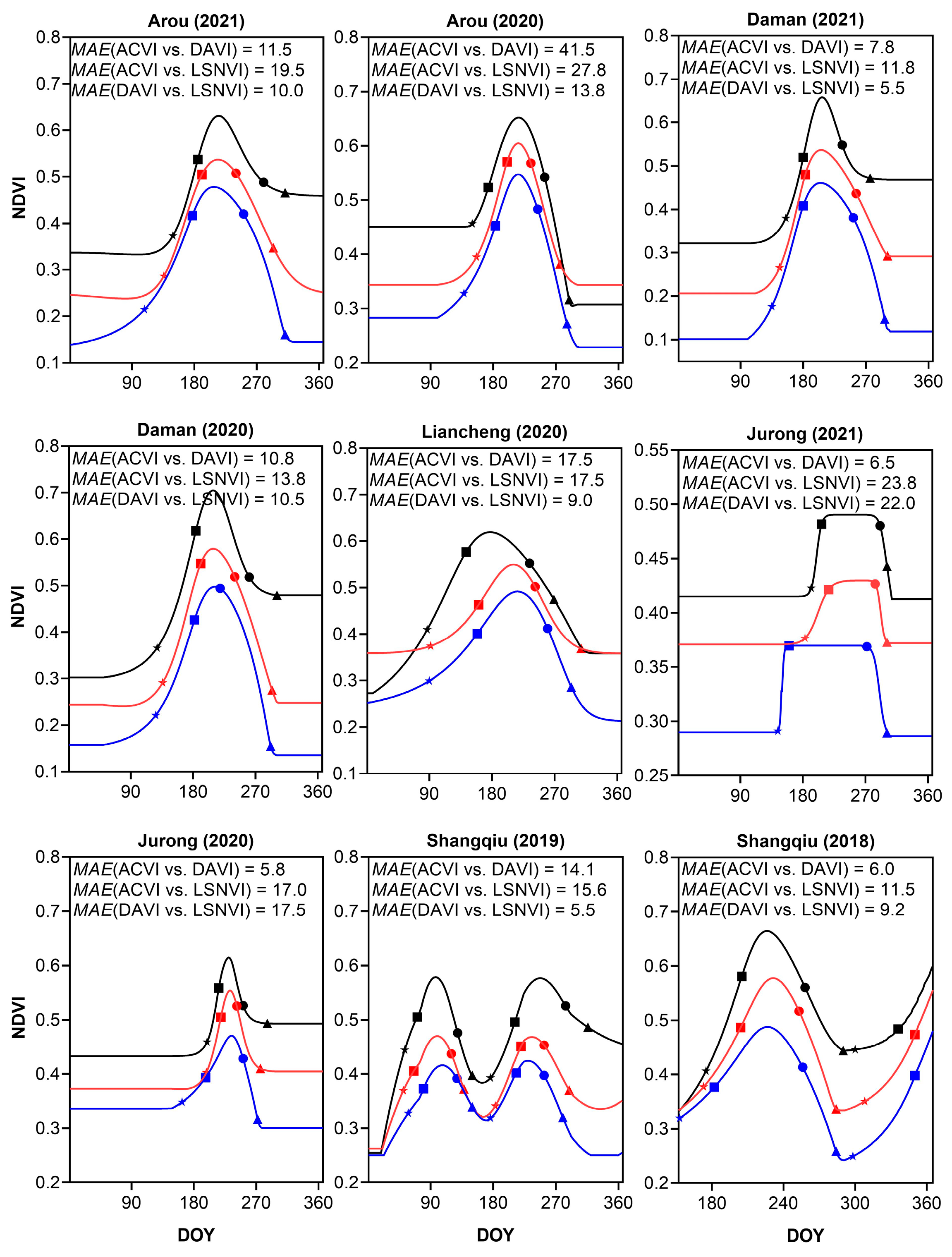
3.4. Comparison Results of PTDs Derived from Different VIs

The MAEs of PTD calculated for the five sites are presented in Figure 7. The time series of LSNVI exhibited the lowest values among all sites, followed by DAVI, and the highest values were observed with ACVI. The MAE of the PTDs extracted by LSNVI and DAVI was lower (5.5 days for Daman and Shangqiu), while the MAE was higher for ACVI compared with LSNVI and DAVI. The MAE for the PTDs in Arou in 2020 could exceed 41.5 days.
The PTDs extracted from the time series of NDVI through various reconstruction methods were compared with the PTDs obtained from the time series GCC, and the results are presented in Figure 8a. Furthermore, we also compared the accuracy of PTDs obtained from retrieved LSNVI and actual LSNVI, with the results shown in Figure 8b. This figure demonstrates that the accuracy of the LSNVI is the highest, followed by DAVI. The RMSE of PTDs derived from LSNVI is 3 days lower than DAVI and 13 days lower than ACVI. Additionally, the RMSE of PTDs derived from retrieved LSNVI is approximately 9 days lower than that of actual LSNVI.

4. Discussion

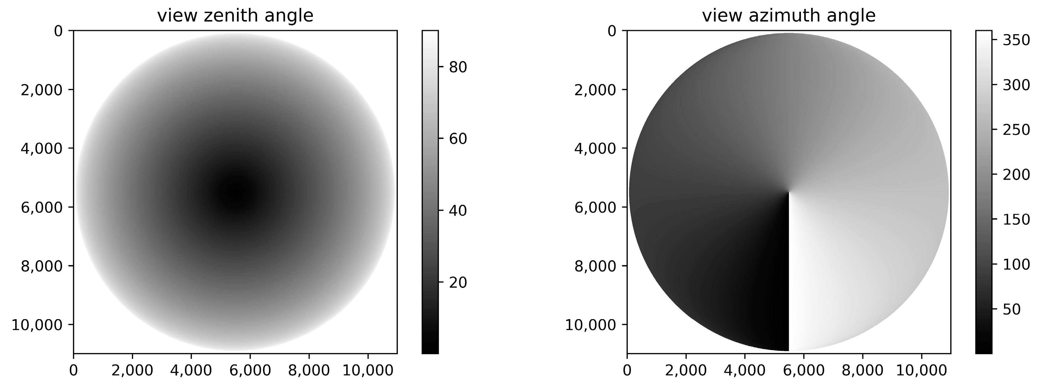
4.1. Impacts of Solar Angles on Geostationary Satellite Data

NDVI obtained from satellite observations can be influenced by the surface BRDF effect. However, previous research has mainly focused on how differences in the viewing angle (VZA and VAA) affect the NDVI [27,29]. The BRDF effect of geostationary satellites has been reported [24], and multiple intraday observations make it possible to study the effect of solar angle variations on the observed NDVI. We used the PROSAIL model to simulate the variation in NDVI with changes in solar angles throughout the day under different LAI conditions (Figure 3). Moreover, we simulated the red and NIR band’s surface reflectance using the MODIS BRDF parameters (MCD43A1) [41] and calculated the corresponding NDVI based on the Ross–Li kernel-driven BRDF model [38]. And then, we made a comparison with the fitted NDVI at different times during the day. The results are shown in Figure 9.
While there are variations in the absolute values of the fitted and modeled NDVIs, as observed at the Arou site, these discrepancies may stem from disparities in the spectral settings of MODIS and FY-4 AGRI, along with biases arising from the extension of the MODIS BRDF parameter product to reflectance simulations at increased solar angles [41]. Despite these differences, both models yield consistent trends in diurnal NDVI, indicating that a decreased SZA corresponds to a lower NDVI under identical viewing conditions. Consequently, a smaller SZA corresponds to a reduced NDVI under the same viewing angle. The impact of BRDF on geostationary satellite observations is crucial. Analyzing multiple intra-day observations from geostationary satellites to derive NDVI highlights a noticeable NDVI variation primarily driven by solar angle (SZA and SAA) variation. Both simulated experiments and actual geostationary satellite observations demonstrate how, in vegetated areas, the lowest NDVI tends to occur near local solar noon when SZA is at its minimum. Conversely, the highest NDVI occurs in the early morning and late afternoon when the SZA is at its peak.
When the SZA is large, a greater portion of the canopy is exposed to sunlight, reducing the proportion of shadow and gaps within the field of view. This results in enhanced vegetation information, leading to a higher NDVI value at a larger SZA [26,29,42]. Conversely, a smaller SZA exposes more of the canopy’s shadow and gaps to sunlight, increasing the background information from the soil and consequently decreasing the NDVI. It is likely that the lowest NDVI for the local solar noon on the day made the proposed model underestimate LSNVI. In Figure 5, the retrieved LSNVI at all sites had a certain underestimation; the bias of the retrieved LSNVI and the actual LSNVI was always negative in all sites in the study year. The time series of LSNVI on all sites was also lower than the ACVI and DAVI (Figure 6).
Furthermore, different vegetation types may demonstrate varying relationships with LSNVI modeling. Data collected from two crop sites, Shangqiu and Jurong, during the sowing period of winter wheat in May and April, revealed that the proportion of vegetation canopy exposed to sunlight remained relatively constant throughout the day. This stability minimized the impact of the changing solar zenith angle (SZA) on the pattern of canopy NDVIs. Consequently, the RMSEs of Shangqiu and Jurong were typically 0.02 higher (Figure 4) when compared to non-crop sites, such as meadows and grasslands.
The utilization of the same fitting and extraction technique for distinct time series NDVIs yields diverse outcomes in vegetation phenological extraction. The impact of clouds is evaded by extracting the average value within a day. However, owing to the influence of surface BRDF, the NDVIs of varied vegetation can be present at different observation moments within a day due to multiple factors, thereby obscuring the regularity and posing a challenge to vegetation phenological extraction. Additionally, through the BRDF correction of reflectance and the subsequent calculation of NDVI with fixed parameters, the adaptability of the correction parameters to different data remains unclear, leading to fluctuations in the calculated NDVI and ultimately impacting the extraction results. The extraction of vegetation phenology often requires obtaining the VI throughout the entire growing season. In our study, we took multiple observations in a day to estimate the NDVI at the local solar noon. Although the SAA of the NDVI was fixed, the variation in SZA during the vegetation growing season needs to be considered in further studies.

4.2. Reconstructing NDVI at the Time of Cloud Cover with Cloud-Free NDVI at Other Time

The algorithm proposed uses cloud-free observations of a pixel during the day to retrieve the NDVI at local solar noon. When there are clouds at local solar noon during the day and no clouds at other times for a pixel, it is possible to estimate the NDVI under the clouds well and thus avoid the influence of clouds to obtain more observations. We compared the count of cloud-free observation days at local solar noon with the cloud-free days in the retrieved time series LSNVI. Figure 10 revealed that the reconstructed time series of NDVI has a higher number of cloud-free days compared with the actual observed cloud-free days, with an average improvement of 34.19%. In particular, the Jurong site exhibited a 51.56% increase in the number of cloud-free LSNDVI days in 2020.
The utilization of high-frequency, cloud-free satellite observations can significantly enhance the precision of vegetation phenology inversions [9,10]. In our study, we reconstructed the cloud cover of LSNVI using the cloud-free NDVI data throughout the diurnal cycle, resulting in a more extensive time-series LSNVI dataset. High-frequency, cloud-free time-series NDVI data substantially improve the accuracy of the phenological transition dates’ (PTDs’) inversion. Specifically, the RMSE of PTDs derived from the estimated LSNVI was approximately 9 days lower than that of the actual LSNVI (Figure 8).

4.3. Other Factors Affecting LSNVI Retrieval Modeling

Several variables may also have an impact on the stability of the LSNVI inversion model. One of these variables is the spatial resolution of the FY-4 AGRI image. The coarse spatial resolution of geostationary satellites makes it challenging to validate the phenology results obtained from these satellites as they do not offer a detailed representation of ground station phenology observations. Several sites in southern China, such as Jurong and Shangqiu, have diverse vegetation structures and patchy land parcels. The 1 km spatial resolution FY-4 AGRI data can result in the “mixed pixel” effect on the surface, thereby making the daily variation pattern of surface NDVI not very clear. As shown in Figure 4, the LSNVI inversion model demonstrated the relatively poor modeling of Jurong in southern China, Shangqiu, and Jurong compared with the northern homogeneous sites. The RMSEs for these southern sites were, on average, 0.02 higher. As a result, the regional mixing of the crops helps mitigate the impact of the BRDF effect on the diurnal variation in NDVI [43].
Furthermore, the precision of cloud identification plays a crucial role in determining the effectiveness of the NDVI input used to calibrate the model parameters, thereby directly impacting the accuracy of the LSNVI inversion. Our algorithm involves utilizing only the 1st, 2nd, and 5th bands of data from the FY-4 AGRI surface reflectance dataset. While this approach is relatively straightforward in the field of geostationary satellite cloud identification [18,25], it contributes to the irregularity observed in the temporal LSNVI for the cloudy sites in the southern region, as shown in Figure 6.
Secondly, the change in the amount of light area covered by the vegetation canopy is strongly influenced by the topographic conditions [44,45]. In addition to the change in the solar angle, the flat topography of the site was selected for this study. Therefore, incorporating topographic factors into the LSNVI inversion model would be a good choice. Additionally, as the study was limited to only five sites in temperate ecosystems, the findings may not fully capture the effectiveness of FY-4 AGRI data in vegetation monitoring. To obtain a more comprehensive understanding, future research should consider using reference data from various types of ecosystems. In future work, combining polar-orbiting satellite data with geostationary satellite data to generate NDVI datasets that have a higher spatial and temporal resolution, as well as consistent illumination-viewing geometry, would be an efficient method.

5. Conclusions

Geostationary satellites can capture multiple observations in a single day, increasing the likelihood of obtaining cloud-free observations. This leads to more usable data for monitoring vegetation phenology. However, the diurnal variation in the solar angle causes the geostationary satellite data to exhibit a noticeable BRDF effect. This introduces uncertainty in the estimation of NDVI. To tackle this issue, we proposed a method that involves normalizing the multiple observed NDVIs to a fixed time, specifically estimating NDVI based on geostationary satellite data at the local solar noon of each day. By standardizing the NDVI acquisition time, we can extract vegetation phenology information from the NDVI values at the local solar noon. To highlight the advantages of our method, we compared it with two other time series NDVI reconstruction methods. These included the angular normalization method for geostationary satellite data, which can enhance the accuracy of time series NDVI in vegetation monitoring.
The BRDF effect is evident even in geostationary satellite observations. When multiple intra-day observations are utilized to derive NDVI from geostationary satellites, a distinct variation in NDVI is observed, primarily influenced by the variation in solar angles (SZA and SAA). Both simulated experiments and actual geostationary satellite observations indicate that in vegetated areas, the lowest NDVI values tend to occur around noon when the SZA is at its minimum. Conversely, the highest NDVI values occur in the early morning and late afternoon when the SZA is larger.
The application of the same fitting and extraction method to the different time series of NDVI often yields varied results in vegetation phenological extraction. While the influence of clouds can be mitigated by extracting the mean value within a day, the surface bidirectional reflectance distribution function (BRDF) introduces complexities. NDVI values of different vegetation types may vary at different observation times due to various factors associated with BRDF, posing challenges to consistent phenological extraction. Furthermore, the BRDF correction of reflectance followed by the NDVI calculation using fixed parameters may result in fluctuating NDVI values due to uncertainties in parameter adaptability across different datasets. To address these challenges, we propose a method for reconstructing NDVI using the local solar noon, effectively reducing the BRDF effect. By developing an empirical model of NDVI changes throughout the day based on cloud-free observations, NDVI can be reconstructed for the cloud-free local solar noon. This approach mitigates the intra-day angle effect on NDVI, ensuring consistency over time and improving the accuracy of phenology extraction.
Vegetation phenology extraction typically necessitates obtaining vegetation indices (VI) throughout the entire growing season. In our study, we conducted multiple observations per day to estimate the NDVI at the local solar noon. While we fixed the solar azimuth angle (SAA) of the NDVI, we did not account for the variation in solar zenith angle (SZA) during the vegetation growing season. Moreover, the coarse spatial resolution of geostationary satellites poses challenges in validating phenology results, as they do not offer a detailed representation of ground station phenology observations. In future research, a promising approach would be to combine polar-orbiting satellite data with geostationary satellite data. This integration could generate NDVI datasets with higher spatial and temporal resolutions as well as consistent illumination-viewing geometry, enhancing the efficiency and accuracy of phenology extractions.
The change in the amount of light area covered by vegetation canopy is significantly influenced by topographic conditions. In addition to changes in solar angle, the flat topography of the site selected for our study underscores the importance of incorporating topographic factors into LSNVI inversion models. Furthermore, as our study was confined to just five sites located in temperate ecosystems, it might not have fully captured the effectiveness of FY-4 AGRI data in vegetation monitoring. To gain a more comprehensive understanding, future research should consider incorporating reference data from a broader range of ecosystem types.

Author Contributions

T.H. and D.-X.S. designed the study; J.L. and C.-Q.W. collected the data, processed the satellite images, and performed the experiments; J.L. conducted the analysis and drafted the manuscript; and T.H., D.-X.S., and C.-Q.W. revised the manuscript. All authors have read and agreed to the published version of the manuscript.

Funding

This research was funded by the National Natural Science Foundation of China, grant number 42271404 and the Open Fund of Key Laboratory of National Geographical Census and Monitoring, Ministry of Natural Resources, grant number 2022NGCM07.

Data Availability Statement

The in situ digital photographs can be accessed at the National Qinghai–Tibetan Plateau Scientific Data Center (TPDC), https://data.tpdc.ac.cn, accessed on 1 May 2024 and the PhenoCam network, https://phenocam.nau.edu/webcam/, accessed on 1 May 2024. The FY-4 AGRI surface reflectance data can be accessed at the Fengyun Satellite Data Center, http://data.nsmc.org.cn, accessed on 1 May 2024.

Acknowledgments

The authors would like to thank the Fengyun Satellite Data Center and the National Tibetan Plateau/Third Pole Environment Data Center.

Conflicts of Interest

The authors declare no conflicts of interest.

References

  1. Zeng, L.; Wardlow, B.D.; Xiang, D.; Hu, S.; Li, D. A review of vegetation phenological metrics extraction using time-series, multispectral satellite data. Remote Sens. Environ. 2020, 237, 111511. [Google Scholar] [CrossRef]
  2. Richardson, A.D.; Keenan, T.F.; Migliavacca, M.; Ryu, Y.; Sonnentag, O.; Toomey, M. Climate change, phenology, and phenological control of vegetation feedbacks to the climate system. Agric. For. Meteorol. 2013, 169, 156–173. [Google Scholar] [CrossRef]
  3. Piao, S.; Liu, Q.; Chen, A.; Janssens, I.A.; Fu, Y.; Dai, J.; Liu, L.; Lian, X.; Shen, M.; Zhu, X. Plant phenology and global climate change: Current progresses and challenges. Glob. Chang. Biol. 2019, 25, 1922–1940. [Google Scholar] [CrossRef] [PubMed]
  4. Smith, W.K.; Dannenberg, M.P.; Yan, D.; Herrmann, S.; Barnes, M.L.; Barron-Gafford, G.A.; Biederman, J.A.; Ferrenberg, S.; Fox, A.M.; Hudson, A.; et al. Remote sensing of dryland ecosystem structure and function: Progress, challenges, and opportunities. Remote Sens. Environ. 2019, 233, 111401. [Google Scholar] [CrossRef]
  5. Chen, M.; Griffis, T.J.; Baker, J.; Wood, J.D.; Xiao, K. Simulating crop phenology in the Community Land Model and its impact on energy and carbon fluxes. J. Geophys. Res. Biogeosci. 2015, 120, 310–325. [Google Scholar] [CrossRef]
  6. Peng, D.; Wang, Y.; Xian, G.; Huete, A.R.; Huang, W.; Shen, M.; Wang, F.; Yu, L.; Liu, L.; Xie, Q.; et al. Investigation of land surface phenology detections in shrublands using multiple scale satellite data. Remote Sens. Environ. 2021, 252, 112133. [Google Scholar] [CrossRef]
  7. Zhang, X. Reconstruction of a complete global time series of daily vegetation index trajectory from long-term AVHRR data. Remote Sens. Environ. 2015, 156, 457–472. [Google Scholar] [CrossRef]
  8. Zhang, X.; Friedl, M.A.; Schaaf, C.B.; Strahler, A.H.; Hodges, J.C.F.; Gao, F.; Reed, B.C.; Huete, A.R. Monitoring vegetation phenology using MODIS. Remote Sens. Environ. 2003, 84, 471–475. [Google Scholar] [CrossRef]
  9. Zhang, X.; Liu, L.; Liu, Y.; Jayavelu, S.; Wang, J.; Moon, M.; Henebry, G.M.; Friedl, M.A.; Schaaf, C.B. Generation and evaluation of the VIIRS land surface phenology product. Remote Sens. Environ. 2018, 216, 212–229. [Google Scholar] [CrossRef]
  10. Zhang, X.; Liu, L.; Yan, D. Comparisons of global land surface seasonality and phenology derived from AVHRR, MODIS, and VIIRS data. J. Geophys. Res. Biogeosci. 2017, 122, 1506–1525. [Google Scholar] [CrossRef]
  11. Armitage, R.P.; Ramirez, F.A.; Danson, F.M.; Ogunbadewa, E.Y. Probability of cloud-free observation conditions across Great Britain estimated using MODIS cloud mask. Remote Sens. Lett. 2013, 4, 427–435. [Google Scholar] [CrossRef]
  12. Zhang, X.; Friedl, M.A.; Schaaf, C.B. Sensitivity of vegetation phenology detection to the temporal resolution of satellite data. Int. J. Remote Sens. 2009, 30, 2061–2074. [Google Scholar] [CrossRef]
  13. Quesada-Ruiz, S.; Chu, Y.; Tovar-Pescador, J.; Pedro, H.T.C.; Coimbra, C.F.M. Cloud-tracking methodology for intra-hour DNI forecasting. Sol. Energy. 2014, 102, 267–275. [Google Scholar] [CrossRef]
  14. Chow, C.W.; Belongie, S.; Kleissl, J. Cloud motion and stability estimation for intra-hour solar forecasting. Sol. Energy 2015, 115, 645–655. [Google Scholar] [CrossRef]
  15. Fensholt, R.; Anyamba, A.; Huber, S.; Proud, S.R.; Tucker, C.J.; Small, J.; Pak, E.; Rasmussen, M.O.; Sandholt, I.; Shisanya, C. Analysing the advantages of high temporal resolution geostationary MSG SEVIRI data compared to polar operational environmental satellite data for land surface monitoring in Africa. Int. J. Appl. Earth Obs. Geoinf. 2011, 13, 721–729. [Google Scholar] [CrossRef]
  16. Yan, D.; Zhang, X.; Yu, Y.; Guo, W. A comparison of tropical rainforest phenology retrieved from geostationary (SEVIRI) and polar-orbiting (MODIS) sensors across the Congo Basin. IEEE Trans. Geosci. Remote Sens. 2016, 54, 4867–4881. [Google Scholar] [CrossRef]
  17. Tian, J.; Zhu, X.; Chen, J.; Wang, C.; Shen, M.; Yang, W.; Tan, X.; Xu, S.; Li, Z. Improving the accuracy of spring phenology detection by optimally smoothing satellite vegetation index time series based on local cloud frequency. ISPRS J. Photogramm. Remote Sens. 2021, 180, 29–44. [Google Scholar] [CrossRef]
  18. Zhao, Y.; Wang, M.; Zhao, T.; Luo, Y.; Li, Y.; Yan, K.; Lu, L.; Tran, N.N.; Wu, X.; Ma, X. Evaluating the potential of H8/AHI geostationary observations for monitoring vegetation phenology over different ecosystem types in northern China. Int. J. Appl. Earth Obs. Geoinf. 2022, 112, 102933. [Google Scholar] [CrossRef]
  19. Miura, T.; Nagai, S.; Takeuchi, M.; Ichii, K.; Yoshioka, H. Improved characterisation of vegetation and land surface seasonal dynamics in central Japan with Himawari-8 hypertemporal data. Sci Rep. 2019, 9, 15692. [Google Scholar] [CrossRef]
  20. Hashimoto, H.; Wang, W.; Dungan, J.L.; Li, S.; Michaelis, A.R.; Takenaka, H.; Higuchi, A.; Myneni, R.B.; Nemani, R.R. New generation geostationary satellite observations support seasonality in greenness of the Amazon evergreen forests. Nat. Commun. 2021, 12, 684. [Google Scholar] [CrossRef]
  21. Wheeler, K.I.; Dietze, M.C. Improving the monitoring of deciduous broadleaf phenology using the Geostationary Operational Environmental Satellite (GOES) 16 and 17. Biogeosciences 2021, 18, 1971–1985. [Google Scholar] [CrossRef]
  22. Yan, D.; Zhang, X.; Nagai, S.; Yu, Y.; Akitsu, T.; Nasahara, K.N.; Ide, R.; Maeda, T. Evaluating land surface phenology from the Advanced Himawari Imager using observations from MODIS and the Phenological Eyes Network. Int. J. Appl. Earth Obs. Geoinf. 2019, 79, 71–83. [Google Scholar] [CrossRef]
  23. Tran, N.N.; Huete, A.R.; Nguyen, H.; Grant, I.; Miura, T.; Ma, X.; Lyapustin, A.; Wang, Y.; Ebert, E. Seasonal comparisons of Himawari-8 AHI and MODIS vegetation indices over latitudinal Australian grassland sites. Remote Sens. 2020, 12, 2494. [Google Scholar] [CrossRef]
  24. Li, Z.; Roy, D.P.; Zhang, H.K. The incidence and magnitude of the hot-spot bidirectional reflectance distribution function (BRDF) signature in GOES-16 Advanced Baseline Imager (ABI) 10 and 15 minute reflectance over north America. Remote Sens. Environ. 2021, 265, 112638. [Google Scholar] [CrossRef]
  25. Ma, X.; Huete, A.R.; Tran, N.; Bi, J.; Gao, S.; Zeng, Y. Sun-angle effects on remote-sensing phenology observed and modelled using Himawari-8. Remote Sens. 2020, 12, 1339. [Google Scholar] [CrossRef]
  26. Gao, F.; He, T.; Masek, J.G.; Shuai, Y.; Schaaf, C.B.; Wang, Z. Angular effects and correction for medium resolution sensors to support crop monitoring. IEEE J. Sel. Top. Appl. Earth Observ. Remote Sens. 2014, 7, 4480–4489. [Google Scholar] [CrossRef]
  27. Galvão, L.S.; Breunig, F.M.; Santos, J.R.; Moura, Y.M. View-illumination effects on hyperspectral vegetation indices in the Amazonian tropical forest. Int. J. Appl. Earth Obs. Geoinf. 2013, 21, 291–300. [Google Scholar] [CrossRef]
  28. Wheeler, K.I.; Dietze, M.C. A statistical model for estimating midday NDVI from the Geostationary Operational Environmental Satellite (GOES) 16 and 17. Remote Sens. 2019, 11, 2507. [Google Scholar] [CrossRef]
  29. Gao, F.; Jin, Y.F.; Li, X.W.; Schaaf, C.B.; Strahler, A.H. Bidirectional NDVI and atmospherically resistant BRDF inversion for vegetation canopy. IEEE Trans. Geosci. Remote Sens. 2002, 40, 1269–1278. [Google Scholar]
  30. Walthall, C.L.; Norman, J.M.; Welles, J.M.; Campbell, G.; Blad, B.L. Simple quation to approximate the bidirectional reflectance from vegetative canopies and bare soil surfaces. Appl. Opt. 1985, 24, 383–387. [Google Scholar] [CrossRef]
  31. Lunagaria, M.M. Parameter estimation and evaluation of Ross-Li and RPV models for wheat phenophases using hemispherical directional reflectance measurements. Int. J. Remote Sens. 2020, 41, 3627–3651. [Google Scholar] [CrossRef]
  32. Yang, J.; Zhang, Z.; Wei, C.; Lu, F.; Guo, Q. Introduction the new generation of Chinese geostationary weather satellites, Fengyun-4. Bull. Amer. Meteorol. Soc. 2017, 98, 1637–1658. [Google Scholar] [CrossRef]
  33. Hufkens, K.; Melaas, E.K.; Mann, M.L.; Foster, T.; Ceballos, F.; Robles, M.; Kramer, B. Monitoring crop phenology using a smartphone based near-surface remote sensing approach. Agric. For. Meteorol. 2019, 265, 327–337. [Google Scholar] [CrossRef]
  34. Julitta, T.; Cremonese, E.; Migliavacca, M.; Colombo, R.; Galvagno, M.; Siniscalco, C.; Rossini, M.; Fava, F.; Cogliati, S.; di Cella, U.M.; et al. Using digital camera images to analyse snowmelt and phenology of a subalpine grassland. Agric. For. Meteorol. 2014, 198, 116–125. [Google Scholar] [CrossRef]
  35. Liu, S.; Xu, Z.; Che, T.; Li, X.; Xu, T.; Ren, Z.; Zhang, Y.; Tan, J.; Song, L.; Zhou, J.; et al. A dataset of energy, water vapor, and carbon exchange observations in oasis–desert areas from 2012 to 2021 in a typical endorheic basin. Earth Syst. Sci. Data. 2023, 15, 4959–4981. [Google Scholar] [CrossRef]
  36. Ma, X.; Huete, A.R.; Tran, N.N. Interaction of seasonal sun-angle and savanna phenology observed and modelled using MODIS. Remote Sens. 2019, 11, 1398. [Google Scholar] [CrossRef]
  37. Jacquemoud, S.; Verhoef, W.; Baret, F.; Bacour, C.; Zarco-Tejada, P.J.; Asner, G.P.; François, C.; Ustin, S.L. PROSPECT+SAIL models: A review of use for vegetation characterization. Remote Sens. Environ. 2009, 113, S56–S66. [Google Scholar] [CrossRef]
  38. Wanner, W.; Li, X.; Strahler, A.H. On the derivation of kernels for kernel-driven models of bidirectional reflectance. J. Geophys. Res. Atmos. 1995, 100, 21077–21089. [Google Scholar] [CrossRef]
  39. Tian, Y.; Romanov, P.; Yu, Y.; Xu, H.; Tarpley, D. Analysis of vegetation index NDVI anisotropy to improve the accuracy of the GOES-R green vegetation fraction product. In Proceedings of the 30th IEEE International Geoscience and Remote Sensing Symposium (IGARSS) on Remote Sensing—Global Vision for Local Action, Honolulu, HI, USA, 25–30 July 2010. [Google Scholar]
  40. Chen, J.; Jonsson, P.; Tamura, M.; Gu, Z.H.; Matsushita, B.; Eklundh, L. A simple method for reconstructing a high-quality NDVI time-series data set based on the Savitzky-Golay filter. Remote Sens. Environ. 2004, 91, 332–344. [Google Scholar] [CrossRef]
  41. Wang, Z.; Schaaf, C.B.; Sun, Q.; Shuai, Y.; Roman, M.O. Capturing rapid land surface dynamics with Collection V006 MODIS BRDF/NBAR/Albedo (MCD43) products. Remote Sens. Environ. 2018, 207, 50–64. [Google Scholar] [CrossRef]
  42. Li, X.; Weng, Y.; Huang, X.; Wu, Q. Analyzing Sunlight Effect on BRDF Characteristics Using Hyperspectral Data. Remote Sens. 2013, 3, 1143–1156. [Google Scholar]
  43. Chen, X.; Wang, D.; Chen, J.; Wang, C.; Shen, M. The mixed pixel effect in land surface phenology: A simulation study. Remote Sens. Environ. 2018, 211, 338–344. [Google Scholar] [CrossRef]
  44. Ma, Y.; He, T.; Li, A.; Li, S. Evaluation and intercomparison of topographic correction methods based on Landsat images and simulated data. Remote Sens. 2021, 13, 4120. [Google Scholar] [CrossRef]
  45. Ma, Y.; He, T.; Liang, S.; Xiao, X. Quantifying the impacts of DEM uncertainty on clear-sky surface shortwave radiation estimation in typical mountainous areas. Agric. For. Meteorol. 2022, 327, 109222. [Google Scholar] [CrossRef]
Figure 1. The workflow of the PTD extraction and model comparison. The t represents the day of the year (DOY). The NDVIi (i = 1, …, n) represent the cloud-free NDVI obtained during the DOY at different times. Abbreviations used in this flowchart are consistent with those used in the study.
Remotesensing 16 02173 g001
Figure 2. The observation angles of each pixel in the full disk of the FY-4 AGRI image.
Remotesensing 16 02173 g002
Figure 3. Variations in the NDVI during a day in simulated and actual scenarios. (a) The calculated SAAs and SZAs at 120°E, 30°N on 1 August 2020; (b) simulated canopy NDVI under different LAI conditions on 1 August 2020 by the PROSAIL model; (c) the actual SAAs and SZAs on 1 August 2020 at five sites; and (d) daily cloud-free FY-4 NDVI from 1 to 16 August 2020 at five sites.
Remotesensing 16 02173 g003
Figure 4. NDVI fitting results for cloud-free observations at the five sites. The black solid lines represent the fitted function, while the points denote the cloud-free NDVI during the three daytime windows.
Remotesensing 16 02173 g004
Figure 5. Validation results of the retrieval LSNVI and the actual LSNVI.
Remotesensing 16 02173 g005
Figure 6. Time series of LSNVI, DAVI and ACVI at five sites. The blue points are LSNVI, the red points are DAVI, and the black points are ACVI. The statistics index is the standard deviation.
Remotesensing 16 02173 g006
Figure 7. The fitted curves and PTDs (star: greenup; square: maturity; circle: senescence; triangle: dormancy) based on different NDVIs over different sites and years. The blue lines and squares are the time series LSNVI curves and derived PTDs, the red lines and squares are the time series DAVI curves and derived PTDs, and the black lines and squares are the time series ACVI curves and derived PTDs.
Remotesensing 16 02173 g007
Figure 8. The evaluation of PTDs extracted by different time series of NDVI. (a) The comparison of PTDs extracted by LSNVI, DAVI, and ACVI; (b) the comparison of PTDs extracted by the estimated LSNVI and the actual LSNVI.
Remotesensing 16 02173 g008
Figure 9. The comparison of the fitted NDVI and the simulated NDVI at different times during the day on the five sites. The blue squares are the fitted NDVI, and the red squares are the simulated NDVI.
Remotesensing 16 02173 g009
Figure 10. The number of cloud-free observation days in actual and retrieved LSNVI time series.
Remotesensing 16 02173 g010
Table 1. Site information.
Site NameLongitudeLatitudeVZAVAAAltitudePeriod (YYYY.MM)Vegetation Types
Arou100.464°E38.047°N44.3128173.14830332020.01–2021.12grassland
Daman100.372°E38.856°N45.222173.12215562020.01–2021.12cropland
Liancheng102.737°E36.692°N42.6157176.71729032020.01–2020.12meadow
Jurong119.217°E31.807°N40.2538206.165152020.01–2021.12cropland
Shangqiu115.592°E34.520°N41.7774198.755552018.06–2019.12cropland
Table 2. The input of PROSAIL model.
ParameterDescription of ParameterUnitsValue
TypelidfLeaf angle distribution typeN/A2
LIDFaAverage leaf angledegree30
LIDFbLeaf distribution’s bimodalityN/A0
CabChlorophyll a + b concentrationμg/cm240
CarCarotenoid concentrationμg/cm28
AntCarotenoid concentrationμg/cm20
CbrownBrown pigment contentN/A0
CwEquivalent water thicknesscm0.01
CmDry matter contentg/cm20.009
NLeaf structure coefficientN/A1.5
Rsoil1Soil reflectance propertiesN/ADry soil
Rsoil2Soil reflectance propertiesN/AWet soil
psoilSoil reflectance propertiesN/A1
rsoil0Soil reflectance propertiesN/Apsoil × Rsoil1 + (1 − psil)*Rsoil2
LAILeaf area indexN/A0.5, 1.0, 1.5, 2.0, 2.5, 3.0
hspotHotspot parameterN/A0.01
ttsSolar zenith angledegree56.867, 43.901, 31.131, 19.328, 12.175, 17.203, 28.549, 41.220, 54.182, 67.110
ttoView zenith angledegree30
psiRelative azimuth angledegree92.768, 85.015, 74.439, 55.067, 7.111, 48.330, 71.397, 83.048, 91.166, 98.097
Disclaimer/Publisher’s Note: The statements, opinions and data contained in all publications are solely those of the individual author(s) and contributor(s) and not of MDPI and/or the editor(s). MDPI and/or the editor(s) disclaim responsibility for any injury to people or property resulting from any ideas, methods, instructions or products referred to in the content.

