Evaluating Machine-Learning Algorithms for Mapping LULC of the uMngeni Catchment Area, KwaZulu-Natal

Abstract

Analysis of land use/land cover (LULC) in catchment areas is the first action toward safeguarding freshwater resources. LULC information in the watershed has gained popularity in the natural science field as it helps water resource managers and environmental health specialists develop natural resource conservation strategies based on available quantitative information. Thus, remote sensing is the cornerstone in addressing environmental-related issues at the catchment level. In this study, the performance of four machine learning algorithms (MLAs), namely Random Forests (RFs), Support Vector Machines (SVMs), Artificial Neural Networks (ANNs), and Naïve Bayes (NB), were investigated to classify the catchment into nine relevant classes of the undulating watershed landscape using Landsat 8 Operational Land Imager (L8-OLI) imagery. The assessment of the MLAs was based on a visual inspection of the analyst and commonly used assessment metrics, such as user’s accuracy (UA), producers’ accuracy (PA), overall accuracy (OA), and the kappa coefficient. The MLAs produced good results, where RF (OA = 97.02%, Kappa = 0.96), SVM (OA = 89.74%, Kappa = 0.88), ANN (OA = 87%, Kappa = 0.86), and NB (OA = 68.64%, Kappa = 0.58). The results show the outstanding performance of the RF model over SVM and ANN with a significant margin. While NB yielded satisfactory results, its sensitivity to limited training samples could primarily influence these results. In contrast, the robust performance of RF could be due to an ability to classify high-dimensional data with limited training data.

1. Introduction

The catchment areas are important ecological components that provide various ecosystem services that benefit society and biodiversity [1,2]. These include the availability of freshwater for consumption, supporting societal needs such as food production, sport, and recreation, and providing a natural habitat [3,4]. Such essential services can be sustained when the biophysical environment of the catchment areas is sustainably managed. However, natural land cover and freshwater resources in the water catchment areas are threatened by Land use/Land cover (LULC) changes in response to societal demands [5]. It is essential to map and monitor the water catchment landscape dynamics to provide valuable information on the distribution of land use activities in the catchment, which serve as the tool for initiatives whose mandates aim to strike a balance between development and the natural environment in the catchment areas. In addition, this information will help water resource managers and other environmental health practitioners establish environmental management plans and policies based on available information [6,7]. Moreover, the availability of such information is important as it can be used to troubleshoot water quality issues and prompt the identification of land resource degradation [8].

Mapping the land use activities of the water catchment can be achieved by either traditional field observation or remote sensing methods. Remote sensing emerged as a convenient and cost-effective way to provide the spatiotemporal data required to analyse heterogeneous landscapes on a large scale [9]. In addition, the remote sensing data can be systematically stored, maintained, and openly shared to end users. A variety of remote sensing sensors (optical and active sensors) have been utilized to map the LULC in the catchment areas. Akar et al. [10] assessed the influence of the contextual data features and various dimensionality filters, including Discrete Wavelet Transform (DWT), in mapping LULC using Headwall Hyperspec data in Bergama, Turkey. Random forest (RF) and support vector machine (SVM) were employed, and RF and DWT data obtained higher overall accuracy and kappa scores of 88.13% and 0.88, respectively. In comparison, SVM recorded lower accuracy than RF. Lekka et al. [11] have used Environmental Mapping and Analysis Program (EnMAP) imagery data to map the LULC using pixel-based machine learning algorithms (MLAs), such as RF and SVM image classification. Their results showed that the SVM image classifier returned an overall accuracy of 92.6%, while the RF model obtained an overall accuracy of 88.1%. Delogu et al. [12] used PRISMA hyperspectral data with machine learning methods, such as RF, an artificial neural network (ANN), and a convolutional neural network (CNN), to classify land use activities in Naples, Italy. The CNN achieved the best results at 0.973% and 0.968 overall accuracy and Kappa, respectively. As the second-best model, the ANN recorded 0.963% and 0.956, and RF showed the lowest classification accuracy at 0.887% and 0.867, respectively.

Other studies have demonstrated the potential of very high spatial resolution (VHR) multispectral data in providing the same service as hyperspectral data in different terrestrial settings and achieving higher classification accuracies. For instance, James [13] utilized Pleiades-1 imagery to map the LULC in Côte d’Emeraude, France. Maximum likelihood (ML) and SVM algorithms were used to implement the classification. The ML algorithm yielded a higher overall accuracy of 84.64% compared to the SVM algorithm, which only produced a map with an overall accuracy of 76.13%. In Fayoum City, Egypt, Mahmoud et al. [14] evaluated a variety of classifiers in mapping the city land cover classes using PlanetScope imagery. They found the ANN model more accurate with a kappa coefficient of 0.97 compared to Naïve Bayes (NB), SVM, RF, and decision trees (DTs), which recorded 0.93, 0.90, 0.86, and 0.87, respectively.

Some studies explored the capabilities of moderate-to-low-resolution sensors’ capabilities in classifying spatial land use classes. For example, in a comparative study, Ref. [6] employed Landsat-8 (L8-OLI) data and SVM and RF algorithms to map Nkandla Forest cover classes in South Africa. L8-OLI was found to be efficient in mapping the forest cover, and SVM was found to be more accurate, with overall accuracy and kappa records of 95.83% and 0.94 compared to 95.24 and 0.93 achieved by RF, respectively. On the west coast of India, a study by Bayas et al. [15] assessed the efficiency of the MLAs in mapping LULC using Sentinel-2 (S2) imagery. NB, Classification And Regression Trees (CART), gradient tree boost (GTB), and RF MLAs were assessed, and the models achieved an overall accuracy of 81.34%, 90.18%, 91.06%, and 92.14%, respectively. A study by Ouchra et al. [9] also used L8-OLI data to evaluate the capabilities of MLAs in land use analysis in Casablanca, Morocco. The RF, SVM, CART, and GTB algorithms were among the tested methods, and RF showed robust performance with an overall accuracy of 95.42% compared to other classifiers with an overall accuracy of 83%, 91.50%, and 93.46%, respectively. A study by Parashar et al. [16] compared SVM and RF algorithms using S2 datasets with and without spectral indices to analyse the LULC of hilly terrain in Gopeshwar, India. The RF models provided more accurate results in both datasets, with overall accuracy and kappa of 86% and 0.83 for a dataset with only spectral bands and 88% and 0.85 for a dataset with incorporated spectral indices, respectively, while SVM reported the lowest accuracy, with overall accuracy and kappa of 82% and 0.79 for spectral bands and 87% and 0.83 for incorporated indices, respectively. In the Munneru River Basin, India, Loukika et al. [17] explored the performance of the MLAs viz. SVM, RF, and CART were used to map the LULC based on L8-OLI and S2 data. They found S2 and RF to dominate their counterparts. The average overall accuracy for RF, SVM, and CART in L8-OLI was 94.85%, 90.88%, and 82.88%. In comparison, S2 average overall accuracy for RF, SVM, and CART was 95.84%, 93.65%, and 86.48%, respectively. Woldemariam et al. [18] evaluated the MLAs in classifying the land use dynamics using L8-OLI data in the Lake Haramaya catchment, Ethiopia. Object-based image analysis (OBIA), SVM, RF, and ANN were tested, and the SVM dominated other classifiers with an overall accuracy of 94%, while RF and ANN achieved 92% and 89%, respectively, and OBIA reported the lowest overall accuracy at 75%. Dash et al. [19] compared the parametric and non-parametric classifiers in mapping LULC based on L8-OLI data in the Big Sunflower River watershed, United States of America (USA). RF, SVM, and the ML were factored in, and their results showed a robust performance with an overall accuracy (kappa) of 93.5% (0.88) and 88.8% (0.82), with RF displaying the worst performance at 84.6%, (0.72).

The success of land cover mapping is dependent not only on the remote sensing data but also on the classification algorithm utilized. As discussed above, various machine-learning algorithms have been used in the remote sensing field to explain the distribution of spatial features in catchment areas, with varying degrees of accuracy reported. Their performance varies with the biophysical features of the landscapes [15]. Hence, there is no generic approach for LULC classification for all terrestrial landscapes [18]. Therefore, it is vital to compare the MLA models to determine their suitability and sensitivity to different geographic settings [18]. Studies that compare the MLAs in mapping LULC in the case of South African landscapes are still limited, if there are any. Thus, in this study, we have identified four prominent MLAs, namely NB, RF, SVM, and ANN, and conducted a comparative study to map the thematic land use classes of the uMngeni river catchment in KwaZulu Natal using L8-OLI data. The current study aims to (i) map the LULC that defines the uMngeni River catchment area and (ii) compare the performance of four non-parametric pixel-based MLAs in a supervised classification based on L8-OLI data. The study is expected to improve the understanding of LULC configuration over the uMngeni River catchment, a key element in building a LULC change and projection module within the catchment to generate information for water resource management strategies.

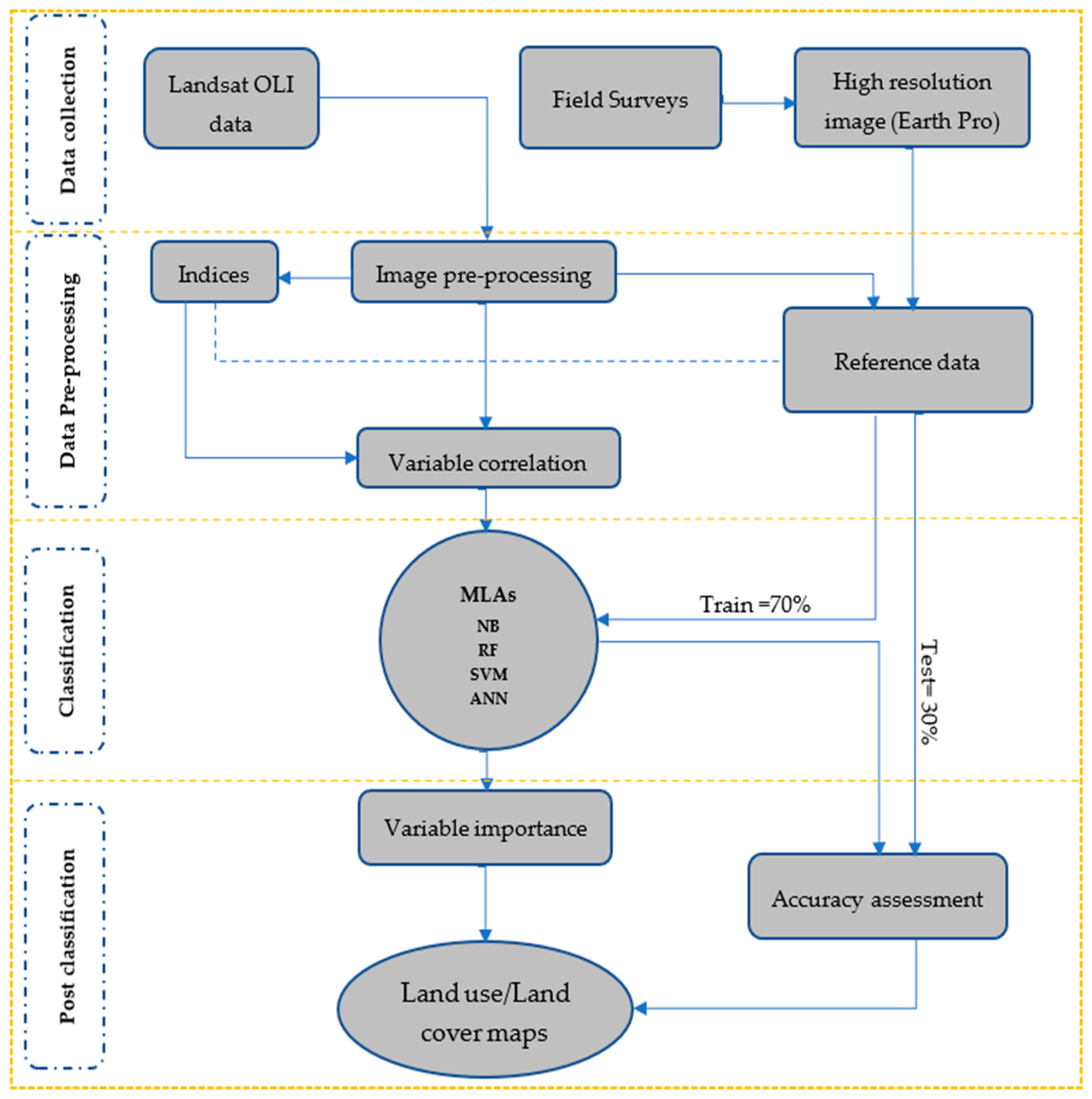
2. Materials and Methods

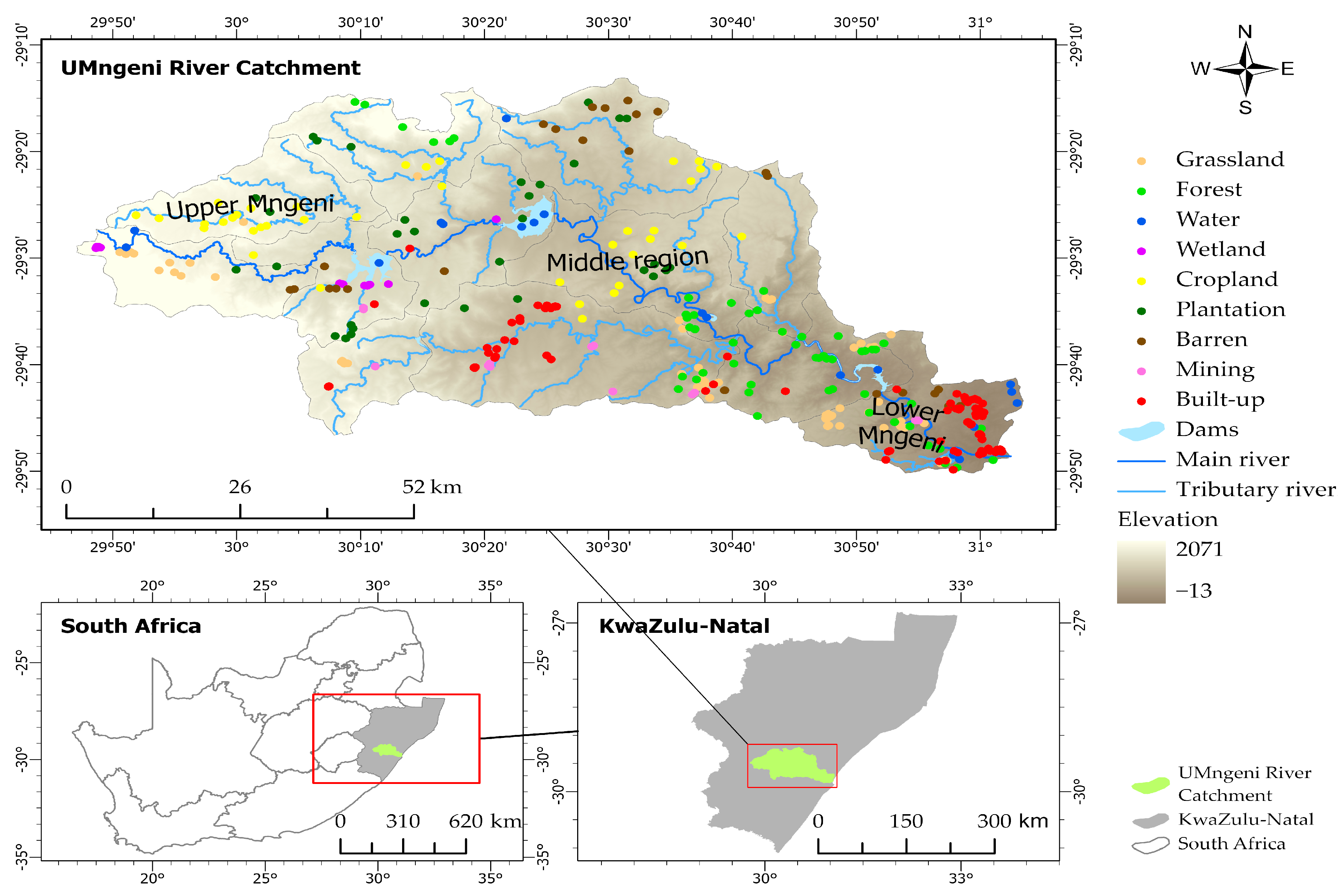
The analysis of the LULC was carried out in a series of steps, as illustrated in Figure 1. The acquired data were preprocessed before implementing the machine learning algorithms, and the LULC was computed. Post-classification analysis was carried out, including accuracy assessment and computing variable importance.

2.1. Study Area

The study area is located in the uMngeni River catchment, KwaZulu-Natal, South Africa (29°29′05.0″S 29°46′52.8″E and 29°48′41.8″S 31°02′27.0″E). The area is situated in the central-western part of KwaZulu-Natal province (Figure 2). It covers 4444 km², which is subdivided into three main regions (lower, middle, and upper) [20]. Its biophysical environment is characterized by a complex river network with an undulating landscape in the upper reaches and gentle slopes with hills towards the lower parts of the catchment, shown in dark color in Figure 2.

The river network forms the uMngeni River, which stretches from the Drakensberg hills in the inner lands of KZN and flows down through Pietermaritzburg, finally depositing in the Indian Ocean via the Durban north estuary. The uMngeni River has four main dams (Midmar, Albert Falls, Nagle, and Inanda), which serve as a water source for 45% of KZN province’s total population [8], including industrial activities, recreation, and agricultural purposes in the cities along the river path, such as Pietermaritzburg and Durban [20]. Land cover change implications not only affect these services but also have an impact on habitat loss, climate change, and biodiversity. To ensure the continuity of such important services, the uMngeni River Catchment was chosen as the study area of interest.

The catchment has an elevation of 1913 m above sea level [21]. Rainfall occurs during the summer (October to March), ranging from 700 to 550 mL per annum. It has moderate temperatures with an annual average of 12 to 20 °C. Its climate and geographic position play a critical role in the province’s economic development. Due to these biophysical characteristics, natural features, and economic activities, the catchment is characterized by a range of land use types.

From our field observation, the land cover types in the catchment include but are not limited to the following: built-up areas, green patches (cropland, plantations, and forests), barren land, and water bodies. Natural vegetation and cropland dominate the uMngeni catchment [8]. Plantations are one of the important land use classes in the catchment and dominate the upper parts of the catchment. The middle part is characterized by heterogeneous patches of different land use types (plantations and built-up areas) [8], while the lower part is mainly dominated by built-up patches with fragments of green vegetated land cover. It is worth unpacking the information in such biodiversity-rich areas to provide updated scientific information.

2.2. Definition of LULC Classes in the Umngeni River Catchment

To assess the LULC in the catchment, a total of nine thematic land use classes were identified, namely built-up areas, cropland, water, plantations, mining, forests, barren, grasslands, and wetlands, as described in

Table 1. Shows The Descriptions of Nine Thematic LULC Classes Used in The Current Study.

Class ID	LULC Classes	Description
1	Grassland	Includes grass and shrubs open areas, as well as golf courses, and sport fields grounds
2	Forest	Natural forests or transition foarest areas rangeing from low to highly dense canopy cover, dominated with trees of appraximately 5 m high.
3	Water	This class considers natural or artificial surface fresh waterbodies within the study area, which includes main rivers and tributries, dams, lakes, and ponds
4	Wetland	This class is mainly made up of hydrphytes and herbaceous species which are solely based on the moisture of the soil to survive. The wetlands can be permanent or temporary depending on the local climate or its size and water holding capacity.
5	Cropland	Composed of both subsistance and ecommercial farming, which might be annual crops, or seasonal. During the post harvest, cultivated lands are charecterised as bare land in the case of seasonal crops.
6	Plantation	Range of tree species cultivated for commercial purposes, this class includes greener patches of the mature trees, sub adult, young, jiviniles, and tree stumps.
7	Barren	Partial vegetated areas, bare land due to either erosion, natural degradation or human factors, post harvest crop fields, dry river banks, and stripped rock areas.
8	Mining	Small patches of mining scars, which comprise of open cast pits, sand mining, and the open raw material processing sites.
9	Built-up	Built-up structures, which includes all forms residential areas, economic corridors, industrial, commercial, educational, religious and health infrastructures.

.

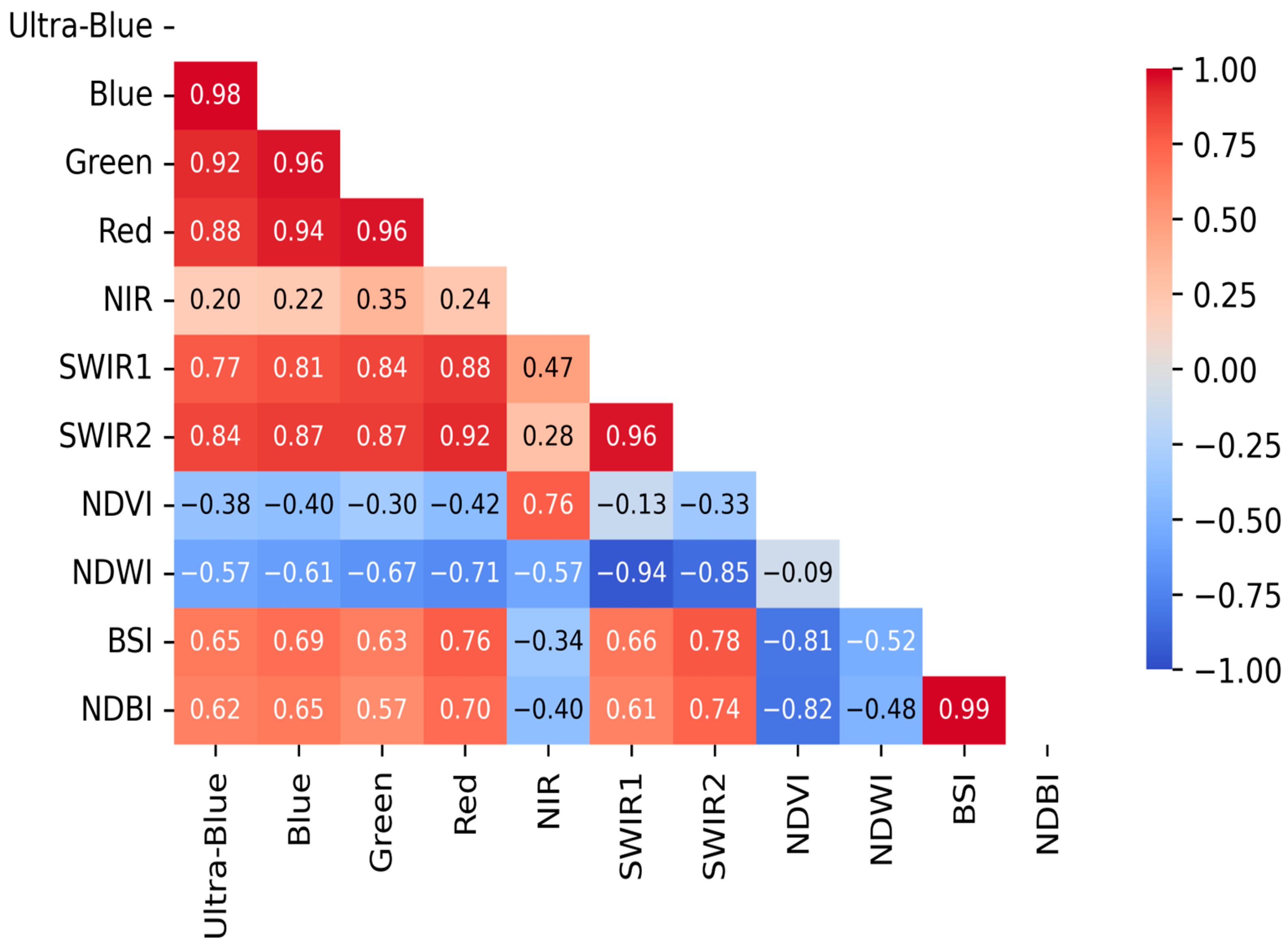
2.3. Remote Sensing Data Acquisition and Preprocessing

In this study, a 30 m resolution image from an L8-OLI image was used for LULC analysis (

Table 2. Details of L8-OLI Spectral Bands and their Respective Spatial Resolutions.

Bands	Wavelength (λ)	Resolution (m)
Blue	0.45–0.51 µm	30 m
Green	0.53–0.59 µm	30 m
Red	0.64–0.67 µm	30 m
Near Infrared (NIR)	0.85–0.87 µm	30 m
Shortwave Infrared 1 (SWIR 1)	1.56–1.65 µm	30 m
Shortwave Infrared 2 (SWIR 2)	2.10–2.29 µm	30 m

). The multispectral image was obtained on 15 May 2023 from the open Google Earth Engine (GEE) data catalog, from the surface reflectance, level 2 category (https://developers.google.com/earth-engine/datasets/catalog/landsat). The surface reflectance category provides images that are ready for analysis with a set of preprocessing requirements that have already been performed to improve the quality of the image [22]. According to [23], surface reflectance images do not require fully blown image preprocessing. Therefore, ee.filter functions were used to set the criteria to select data that meet the needs of the study. It must also be noted that scenes from different dates but in the same season have been collected using ee.Filter.date(). Images from the same season will not have an impact on the analysis since the atmospheric variation is minimal. A total of four scenes (each with a total area of 185 km by 180 km) from two rows and paths were collected to cover our study area. Then, the filterMetadata function was set to return only scenes with a cloud cover of less than 10% [24].

However, the filtering processing alone was infeasible to prepare the image for the analysis. Therefore, image preprocessing was performed as a prerequisite for any satellite image in the GEE interface. The median composite was formed from a series of scenes from the winter season, 01 May to 30 August 2022.

To stretch our specifications, the boundary shape file was used to create a subset of our study area from the composite image using the Clip() function. Then, the subset was subject to further processing, as the clouds are unavoidable in the satellite image [25]; the function of the mask from C code, commonly known as CFmasking, was applied to remove cloud-infested pixels in the image, as used by [26]. The approach involves the quality assurance (QA-PIXEL) band, which assigns zero values to the cloud-contaminated pixels and cloud shadows, producing a cloud-free composite [27].

Calculated Spectral Indices

Spectral indices are derived from the pixel-wise ratios of two or more bands of the multispectral image, which serve as both logistics and added explanatory variables for image classification [28]. Many studies have achieved meaningful LULC classification results by supplementing multispectral bands with information from spectral indices [17,28,29]. The indices layers facilitate the discrimination of specific features and assign the pixels to predicted classes. Our study area possesses diverse spatial attributes, making distinguishing the class members from others difficult. Hence, the current study employed various mathematical equations (

Table 3. Supplementary Indices Used in the Land Use Classification.

Index	Equation	References
NDVI	NDVI $=\frac{NIR - Red}{Red + NIR}$	[30]
NDWI	NDWI $=\frac{Green - NIR}{Green + NIR}$	[32]
BSI	BSI = $\frac{(\left(Red + SWIR\right) - (NIR + Blue\left)\right)}{(\left(Red + SWIR\right) + (NIR + Blue\left)\right)}$	[33]

) to compute the normalized difference indices (NDI) for vegetation (NDVI) [30] to improve the separation of vegetation classes [31], as well as water indices (NDWI) to distinguish waterbodies from hill shadows [32] and bare soil indices (BSI) [33] to identify bare surfaces [34]. These indices were also used as additional explanatory inputs to L8-OLI visible, NIR, and SWIR bands.

2.4. Reference Data Collection

The field survey approach and Google Earth Pro 7.3.6 high-resolution images were used in collecting sampling data for building and measuring the mapping accuracy of the classifiers. The field survey was carried out on 16 August 2023, where coordinates of predefined thematic land use classes (Table 1) were extracted using a portable global positioning system (GPS) through a random sampling method. The same method was also used in Google Earth Pro-based sample collection. This approach widely places the sampling points across the study area (Figure 2) and ensures all the land cover classes are adequately represented in the reference data [35,36]. The GPS coordinates were imported into the Google Earth Pro 7.3.6 platform and overlaid on high-resolution images to locate the land cover classes [37]. Around each coordinate, the irregularly sized polygons were then digitized to represent the corresponding land cover class (

Table 4. Training and Test Samples Used in the Study.

LULC Class	No. of Polygons	Training Pixel Count	Test Pixel Count
Grassland	63	6944	1685
Forest	51	5823	1483
Water	38	1865	435
Wetland	11	357	86
Cropland	38	8965	2163
Plantation	32	7820	1957
Barren	30	4492	1075
Built-up	86	2504	598
Mining	13	667	159
Total	362	39437	9641

). The digitized reference polygons were imported into GEE and overlayed onto an L8-OLI image. Then, the spectral properties of cover classes were extracted from the L8-OLI image per pixel, as shown in Table 4, and randomly divided into two datasets, a training dataset (70%) and a validation data set (30%) [7]. These two datasets were used to train and assess the accuracy of the MLA models—NB, RF, SVM, and ANN.

2.5. Image Classification

Regions with diverse land use classes can make it difficult for machine learning models to discover the relationship between explanatory features [38]. Therefore, before commencing the classification stage, it is important to scrutinize the variables based on their spectral similarities in the given class. To address this, the Pearson correlation coefficient was used to perform variable correlation analysis. It is a commonly used pair-wise technique that helps to identify the collinearity between two variables and eliminate noise [39]. It improves the accuracy of the MLAs by reducing redundancy and improving the computation processing rate. The stepwise correlation analysis was performed on L8-OLI explanatory variables; (1) spectral reflectance information for each variable was extracted from sampling sites, (2) imported into Python to compute variable correlation using the corr() algorithm, and (3) Seaborn’s package was employed to plot the correlation array as a heat map matrix.

2.5.1. Selected Classifiers and Parameter Tuning

Naïve Bayes

The NB classification approach evolved from the Bayesian and Naive theorem. The Bayesian technique assumes the possibility of a recurrence of the event based on learning from the previous event [40], while Naive is a probabilistic classifier with a strong independent assumption of the feature from the others [29]. In other words, dimensions that define a certain variable are independent of each other. Naïve Bayesian theory can be expressed mathematically as the probability of a pixel being in class k given X as a training sample, which is equivalent to the density of the sample size given the class multiplied by the probability of the pixel being in class k and divided by the density of the sample size:

$$\mathrm{P}\left(\mathrm{y}=\mathrm{k}|\mathrm{X}\right)=\frac{\mathrm{p}\left(\mathrm{X}\right|\mathrm{y}=\mathrm{k}\left)\right(\mathrm{P}(\mathrm{y}=\mathrm{k}))}{\mathrm{p}\left(\mathrm{X}\right)}$$

(1)

where y is the unassigned variable, k is the class, and X is the training sample. Therefore, P(y = k|X) is the probability of the y and p is the density. NB models can be trained in supervised classification methods either in the form of parametric or non-parametric models by incorporating Gaussian functions.

The NB model is easy to tune in GEE and lambda (λ) is the only parameter that can be adjusted to avoid assigning zero probability to classes that could not be identified in the training stages [38]. The model computes the statistics (the mean and the variance of the variables for each class) required for classification from the provided training data [15]. In LULC analysis, it has been reported as a promising classifier with satisfactory results [29]. Its performance is attributed to the independence of the feature dimensions from the others. For the purpose of our study, the NB model from the “smileNaiveBayes” library in GEE was used.

Random Forests

The RF classifier is an ensemble classifier that uses regression decision trees to classify the dataset [41]. It gained popularity in the remote sensing community due to its reduced computational processing time, unique classification approach, and robust performance [28]. The RF proposed by Breiman [41] involves bagging the CART split criterion. Bagging facilitates the building of the bootstrap samples from the original training sample data, a process also known as bootstrapping, forming predictor trees from each bootstrap sample. The class membership of the unknown pixel is determined by the votes from all decision trees [7]. The decision to assign the pixels to the class is based on the aggregate (average of the votes) results from multiple RF decision trees [42,43]. The advantage of the RF model is the ability to handle high-dimensional datasets [15] while being insensitive to outliers and overfitting [44]. The RF model excludes some samples for each newly generated tree, commonly known as out-of-bag samples (OOB), which report on the important features in the classification and misclassification errors of each tree [45]. For the model to meet analysts’ needs, requirements must be predefined in the parameter tuning stages.

Two important parameters to be set when building the model are the number of decision trees to be created (Ntree) and the number of variables to be selected per split (Mtry). The higher value of Ntree does not improve the accuracy of the classifier; instead, it brings confusion. A lower Ntree increases the confidence in features used to build the decision trees and reduces the correlation between the electorates [28,44]. In contrast, Ntree can be as large as possible, while Mtry should be equal to the square root of the number of features [46]. There is no standardized way to adjust the parameters for RF models. Therefore, it depends on the discretion of the analyst and the nature of the study. In this study, the RF classifier from the “smileRandomForest” library was utilized. To optimize the model, Ntree was adjusted to 25 and Mtry was set to three, which is equal to the square root of explanatory features, and each node was adjusted to have 2 leaves, as detailed in

Table 5. Hyperparameter Tuning of the MLA Models.

Classifier	Classifiers	Parameters	Parameter Adjustments
NB	ee.Classifier.smileNaiveBayes()	λ	0.000001
RF	ee.Classifier.smileRandomForest()	Ntree	25.00
		Mtry	null
		MinLeafPopulation	2.00
		MaxNodes	1000.00
		BagFraction	0.50%
SVM	ee.Classifier.libsvm()	kernelType	POLY
		svmType	C_SVC
		coef0	0.3
		degree	1.00
		cost	10
ANN	MLPClassifier (ANN)	activation	RELU
		hidden_layer	1.00
		nuerons	10

. Each decision tree received a share of 0.5% from the original sample data for OOB, and nodes per tree were set not to exceed 1000. The optimization of the parameters was obtained using 10-fold cross-validation.

Support Vector Machine

The SVM algorithm is a supervised vector-based classifier that has been used for both regression and classification [47]. Different types of SVM models have been widely used for different remote sensing applications which include LULC, water quality, and vegetation mapping. SVM models use discriminative methods by learning the distribution patterns of training data. It uses linear or nonlinear lines (known as hyperplanes) to optimize the boundaries between the vector data. The development of SVM models was designed as a binary classifier that only deals with linear data [48]. The method uses the principle of finding the best marginal line (hyperplane) between the two features in the high-dimensional space. Then, the optimal hyperplane serves as the decision boundary that separates the two features. This principle generally works well when applied to linear data.

However, it is challenging to separate nonlinear data using the linear SVM approach because the inherent design of its model tends to incompletely separate the training dataset, leading to classification errors [49]. After numerous attempts to develop SVMs suitable for classifying nonlinear data, combined SVM and kernel functions became a viable way to separate nonlinear data. The primary role of the kernel function in SVM models is to mobilize the training data to a new dimensional space, allowing the marginal lines to find the optimal hyperplane to separate the vectors [50]. The most popular kernel functions for the classification of complex remote-sensed data include the radial basis function (RBF) and the polynomial kernel [51]. These two kernels have been reported in the literature for their ability to produce accurate classification results; for example, [52] used RBF-SVM to monitor dynamic land use changes in Urmia Lake Iran, as did [53] in urban expansion mapping using a polynomial kernel function. In addition, [51] compared the performance of the kernels and found RBF to be slightly more accurate than the polynomial kernel in delineating the sub-catchment.

As there is no rule of thumb in kernel selection, the analyst’s discretion is used based on the nature of the study. Therefore, for the current study, the polynomial kernel was selected based on the trial-and-error approach. The applicable SVM type for the polynomial kernel in sensing data analysis is support vector classifier (SVC), which allows for the cost (C) of non-separatable vectors (C-SVC). Thus, it is also known as a soft margin because it requires only the best hyperplane and accepts some separation errors as defined in the C threshold; if value C is high, it can lead to overfitting. In this way, C-SVC guarantees results whose integrity is highly dependent on the training data and parameter tuning of the model (Table 5). The C-SVC model has been used in different studies for LULC classification and achieved meaningful results, such as in [17].

The C-SVC from the “libsvm” library in GEE was used. The kernel and C were set to polynomial and 10, respectively, as the main parameters to control marginal lines and error threshold. Additionally, hyperparameters were also tuned, including a degree, gamma, and coef0, to achieve the optimum hyperplane, as shown in Table 5.

Artificial Neural Network

ANN is a non-parametric algorithm with a complex network of interconnected neurons. The network is composed of an input phase, one or more intermediate phases, and an output phase. In remote sensing applications, the input layer has neurons that serve as receptor sites for data from each variable. They pass the data to the intermediate phase via channels. Each channel has a numeric value assigned, known as weight, which is the factor of the inputs to be transmitted to the neurons of the intermediate phase [54]. Neurons in the intermediate phase house the numeric values called bias, which are added to the inputs. Then, the total neuron values are subjected to the activation function, which determines the neurons that are going to contribute to the inputs of the next phase [55]; all the activated neurons transmit the inputs to the next phase in a process called forward propagation. The inputs are propagated through the network to the output phase, where the inputs are assigned to a corresponding class [56]. In addition, the misclassified data are backpropagated through the network model iteratively for revision by adjusting the weights. In this study, the feed-forward propagation ANN model from the Sci-Kit learn package applicable in Python (Google Colab cloud computing platform) was used, as defined:

$$\mathrm{Output}=\mathrm{a}\mathrm{S}\left({\sum }_{\mathrm{i}-1}^{\mathrm{n}}{\mathrm{w}}_{\mathrm{i}}{\mathrm{w}\mathrm{z}}_{\mathrm{i}}+\mathrm{b}\right)$$

(2)

where w_i and z_i are weights that are carried by the channels, b is the bias as the remainder of the training samples, and i is the number of neurons in the intermediate phase.

According to [57], ANN models, in general, tend to overestimate the classes. The network size and the number of neurons to be used are very important parameters to consider in achieving the best results; a large complex network can lead to overfitting of the input data [58]. The number of intermediates was set to 1 phase with 10 iterations. The nonlinearity was solved by the RELU activation function, as detailed parameter tuning is presented in Table 5.

2.6. Variable Importance

The inherent designs of MLA models are complex in nature, and it is challenging to interpret their interaction with the input data [59]. However, understanding the model’s behaviour is important [60] to determine the utility features and gain insight into the mechanisms of the models [61,62]. Thus, the built models (NB, RF, SVM, and ANN) were further investigated to explain the interaction between models and features in classifying given LULC classes (Table 1) using the Shapley Additive exPlanation (SHAP) value. Its approach is based on game theory, which explains the impact of individual features on the prediction of machine learning models [59]. To compute the SHAP value, the Sci-Kit learn and shap packages in Python were used to build both MLA and SHAP value explainer models, respectively.

2.7. Accuracy Assessment

The most used accuracy assessment standard for land use mapping is the Kappa coefficient [37]. The Kappa coefficient assesses the status of classification results against the randomly assigned values. The nature of the Kappa values ranges from −1 to 1. These kappa values rank the classification accuracy of the classified image; when the value is less than zero, there is no agreement. When the value is ≤0.40, there is a fair amount of accuracy. A value ≤0.75 indicates satisfactory accuracy, and ≤1 indicates good performance [63]. The Kappa coefficient can be defined as follows:

$$\mathrm{K}=\frac{\mathrm{P}\left(\mathrm{A})-\mathrm{P}(\mathrm{E}\right)}{1-\mathrm{P}\left(\mathrm{E}\right)}$$

(3)

where P(A) is the overall accuracy and P(E) is the chance agreement, which is given by the sum of the predicted values and actual values for each class and agreement by chance [64].

Note: j = land use class of interest (e.g., water bodies) and will be used as an example to determine the accuracies of the class of interest.

The overall accuracy represents the sum of correctly labelled pixels for all the classes in the input image as per the provided test sample sites and is mathematically expressed as a fraction of correctly labelled pixels and the total number of test sample sites [65].

$$\mathrm{OA}=\frac{{\sum }_{\mathrm{c}\mathrm{o}\mathrm{r}\mathrm{r}\mathrm{e}\mathrm{c}\mathrm{t}\mathrm{l}\mathrm{y} \mathrm{l}\mathrm{e}\mathrm{b}\mathrm{a}\mathrm{l}\mathrm{l}\mathrm{e}\mathrm{d} \mathrm{p}\mathrm{i}\mathrm{x}\mathrm{e}\mathrm{l}\mathrm{s}}}{{\sum }_{\mathrm{p}\mathrm{i}\mathrm{x}\mathrm{e}\mathrm{l}\mathrm{s} \mathrm{i}\mathrm{n} \mathrm{t}\mathrm{e}\mathrm{s}\mathrm{t} \mathrm{s}\mathrm{a}\mathrm{m}\mathrm{p}\mathrm{l}\mathrm{e} \mathrm{s}\mathrm{i}\mathrm{t}\mathrm{e}\mathrm{s}}}$$

(4)

PA is the number of pixels that the test sample of the given class (j) agreed to labelled pixels as class j in the input image. It is given by the sum of correctly labelled pixels of a class, j, divided by the sum of correctly labelled pixels and the pixels claimed to not belong to class j, as adapted from [37]:

$${\mathrm{P}\mathrm{A}}_{\mathrm{j}}=\frac{{\sum }_{\mathrm{c}\mathrm{o}\mathrm{r}\mathrm{r}\mathrm{e}\mathrm{c}\mathrm{t}\mathrm{l}\mathrm{y} \mathrm{l}\mathrm{e}\mathrm{b}\mathrm{a}\mathrm{l}\mathrm{l}\mathrm{e}\mathrm{d} \mathrm{p}\mathrm{i}\mathrm{x}\mathrm{e}\mathrm{l}\mathrm{s}\mathrm{j}}}{{\sum }_{\mathrm{c}\mathrm{o}\mathrm{r}\mathrm{r}\mathrm{e}\mathrm{c}\mathrm{t} \mathrm{l}\mathrm{e}\mathrm{b}\mathrm{a}\mathrm{l}\mathrm{l}\mathrm{e}\mathrm{d} \mathrm{p}\mathrm{i}\mathrm{x}\mathrm{e}\mathrm{l}\mathrm{s}\mathrm{j} + \mathrm{m}\mathrm{i}\mathrm{s}\mathrm{l}\mathrm{e}\mathrm{b}\mathrm{a}\mathrm{l}\mathrm{l}\mathrm{e}\mathrm{d} \mathrm{a}\mathrm{s} \mathrm{c}\mathrm{l}\mathrm{a}\mathrm{s}\mathrm{s}\mathrm{j}}}$$

(5)

The user’s accuracy is determined by the number of correctly labelled pixels in the class divided by the sum of the pixels in the class claimed to belong to class j in the test samples, as proposed by [66].

$${\mathrm{U}\mathrm{A}}_{\mathrm{j}}=\frac{{\sum }_{\mathrm{c}\mathrm{o}\mathrm{r}\mathrm{r}\mathrm{e}\mathrm{c}\mathrm{t}\mathrm{l}\mathrm{y} \mathrm{l}\mathrm{e}\mathrm{b}\mathrm{a}\mathrm{l}\mathrm{l}\mathrm{e}\mathrm{d} \mathrm{p}\mathrm{i}\mathrm{x}\mathrm{e}\mathrm{l}\mathrm{s}\mathrm{j}}}{{\sum }_{\mathrm{c}\mathrm{o}\mathrm{r}\mathrm{r}\mathrm{e}\mathrm{c}\mathrm{t} \mathrm{l}\mathrm{e}\mathrm{b}\mathrm{a}\mathrm{l}\mathrm{l}\mathrm{e}\mathrm{d} \mathrm{p}\mathrm{i}\mathrm{x}\mathrm{e}\mathrm{l}\mathrm{s}\mathrm{j} + \mathrm{l}\mathrm{e}\mathrm{b}\mathrm{a}\mathrm{l}\mathrm{l}\mathrm{e}\mathrm{d} \mathrm{a}\mathrm{s} \mathrm{c}\mathrm{l}\mathrm{a}\mathrm{s}\mathrm{s}\mathrm{j}}}$$

(6)

In an effort to assess the performance of the NB, RF, SVM, and ANN models, the aforementioned accuracy metrics will be calculated from the confusion matrix of each model.

3. Results

Figure 3 illustrates the result of the L8-OLI variable collinearity test, as discussed in Section 2.3. One variable of the highly correlated pairs was removed. For example, the ultra-blue and blue bands show a linear spectral relationship of 0.98, as shown in the red and light-red cells in Figure 3. In contrast, variables that showed the least correlation or distinct spectral variation were retained to facilitate the classification process. As a result, from a total of eleven tested variables, six multi-spectral bands, such as visible (blue, green, and red), NIR, and SWIR (1 and 2) bands, were selected as explanatory variables for the LULC classification, along with three spectral indices (NDVI, NWDI, and BSI). To demonstrate the unique spectral information of each variable per class, the spectral variability was computed, as illustrated in Figure 4.

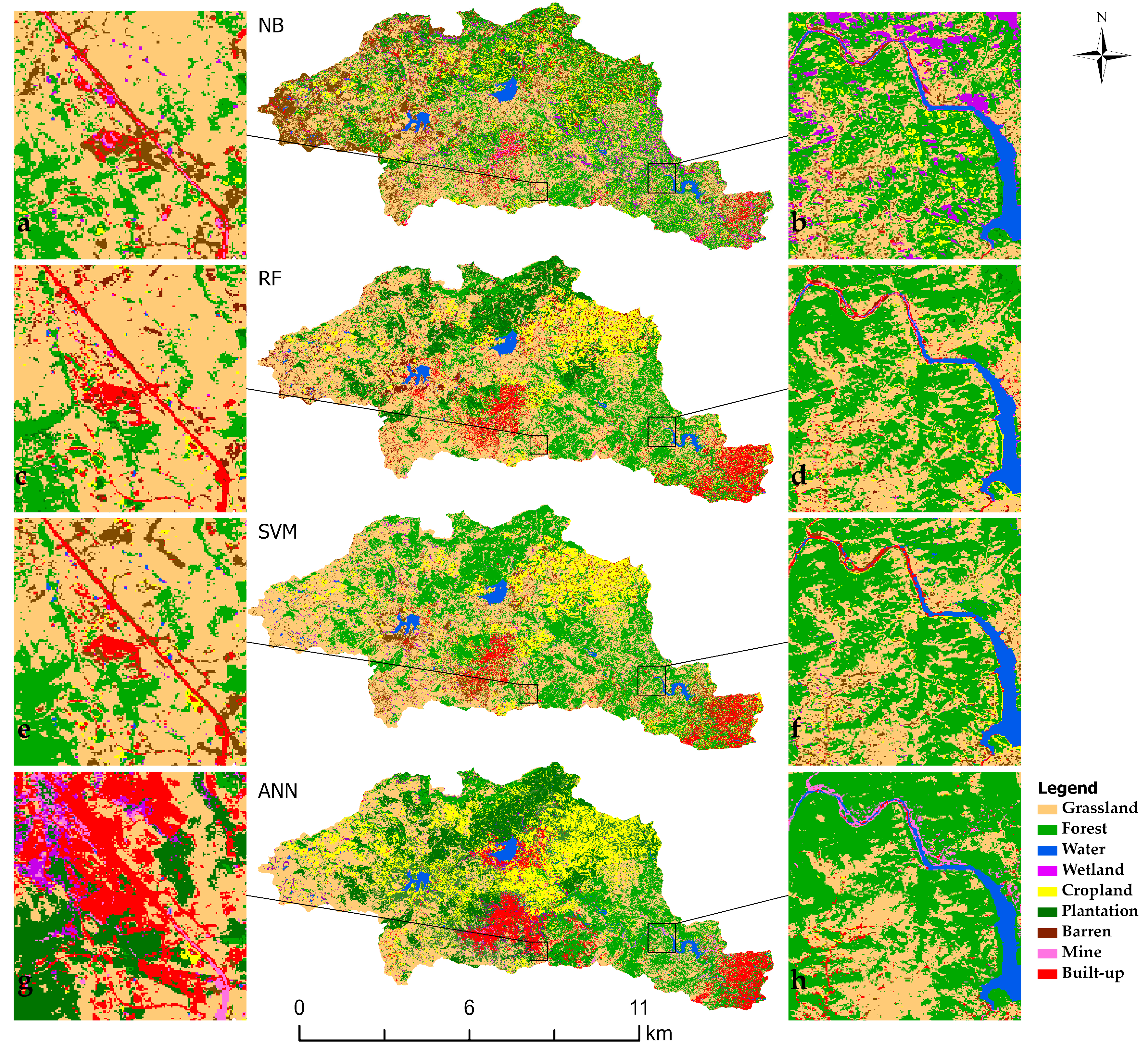
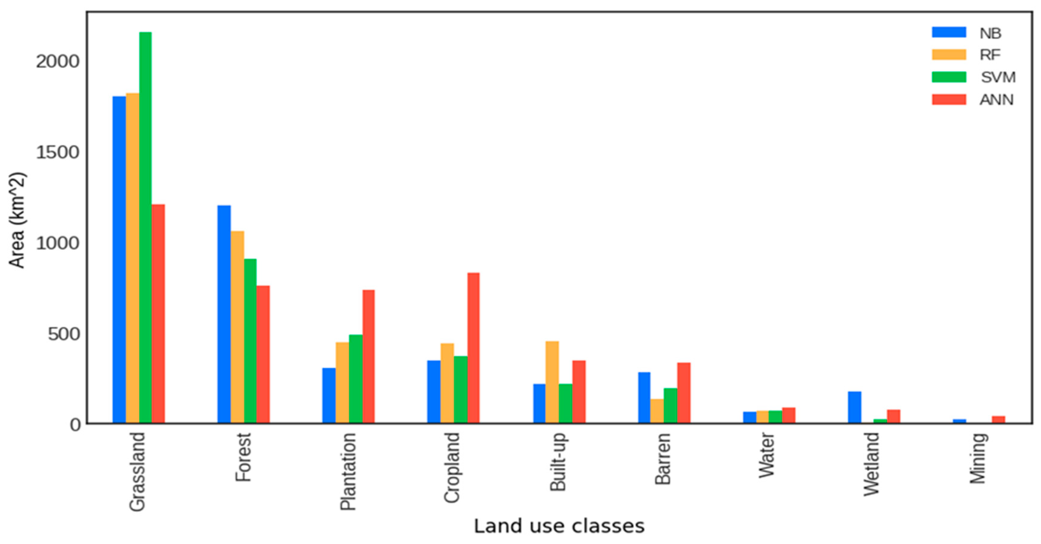
3.1. Mapping and Spatial Extent of LULC Classes

This study successfully mapped nine LULC classes covering about 4444 km² of the uMngeni River catchment using four MLA strategies (NB, RF, SVM, and ANN). The classification results are shown in Figure 5, and the graphical representation is in Figure 6. The MLAs show estimates of varying extent but agree to the class geographic position in the study area. The catchment is dominated by grassland vegetation, covering 1819.31 km² (RF) and 1206.16 km² (ANN). Natural Forest is the second dominant class, with an area cover of 1200.13 km² determined by NB and 762.2 km² by ANN. This is followed by planted forest, with an estimate of 738.9 km² and 296.5 km² by NB.

Plantation, as the third dominant class, shows slight variations in area cover in NB, SVM, and RF (Figure 6), while there was a distinct area coverage of 738.88 km² recorded by the ANN model. ANN showed a significant area extent of 831.27 km² in the cropland class. In contrast, RF and SVM reported statistically insignificant areas for cropland class cover at 372.73 km² and 440.29 km², respectively. Built-up and bare soil area cover vary across the four MLAs, ranking them in the fifth and sixth dominant classes. The water, wetland, and mining classes showed the least area coverage. In this category, the mining class represents the least coverage of the total study area, with an area cover at a maximum of 45.04 km² as determined by ANN (Figure 6).

The geographic positions of thematic land use classes are consistent across four MLAs (Figure 5). In the grassland matrix, which dominates the catchment by 40.99%, cropland and barren land are observed in the proximal distance from the water bodies and in the periphery of the upper parts of the catchment. Meanwhile, natural forest land covers a large portion of the middle reaches and extends to the lower regions, with about 0.08% of mining classes on the forest banks. The plantation is scattered around the upper region, with higher density in the far north of the upper region. The distribution of 10.27% (

Table 6. Cover Areas of Thematic Land Use Classes as Reported by RF ¹.

LULC Class	Area in km2	Area in %
Grassland	1819.31	40.94
Forest	1058.55	23.82
Built-up	455.69	10.25
Cropland	446.49	10.05
Plantation	440.29	9.91
Barren	134.68	3.03
Water	74.81	1.68
Wetland	5.29	0.12
Mining	3.35	0.08
Total	4444.00	100.00

¹ These are the results (km² and percentage) for class area cover that were used in the Discussion section since RF produced more accurate maps than SVM, NB, and ANN.

) of the built-up class is observed mainly in the lower region of the study area, with dense areas towards the uMngeni river estuary (Figure 6). The wetland class covered tiny patches (0.12%) in the dam shorelines and was visible at the tip of the upper region.

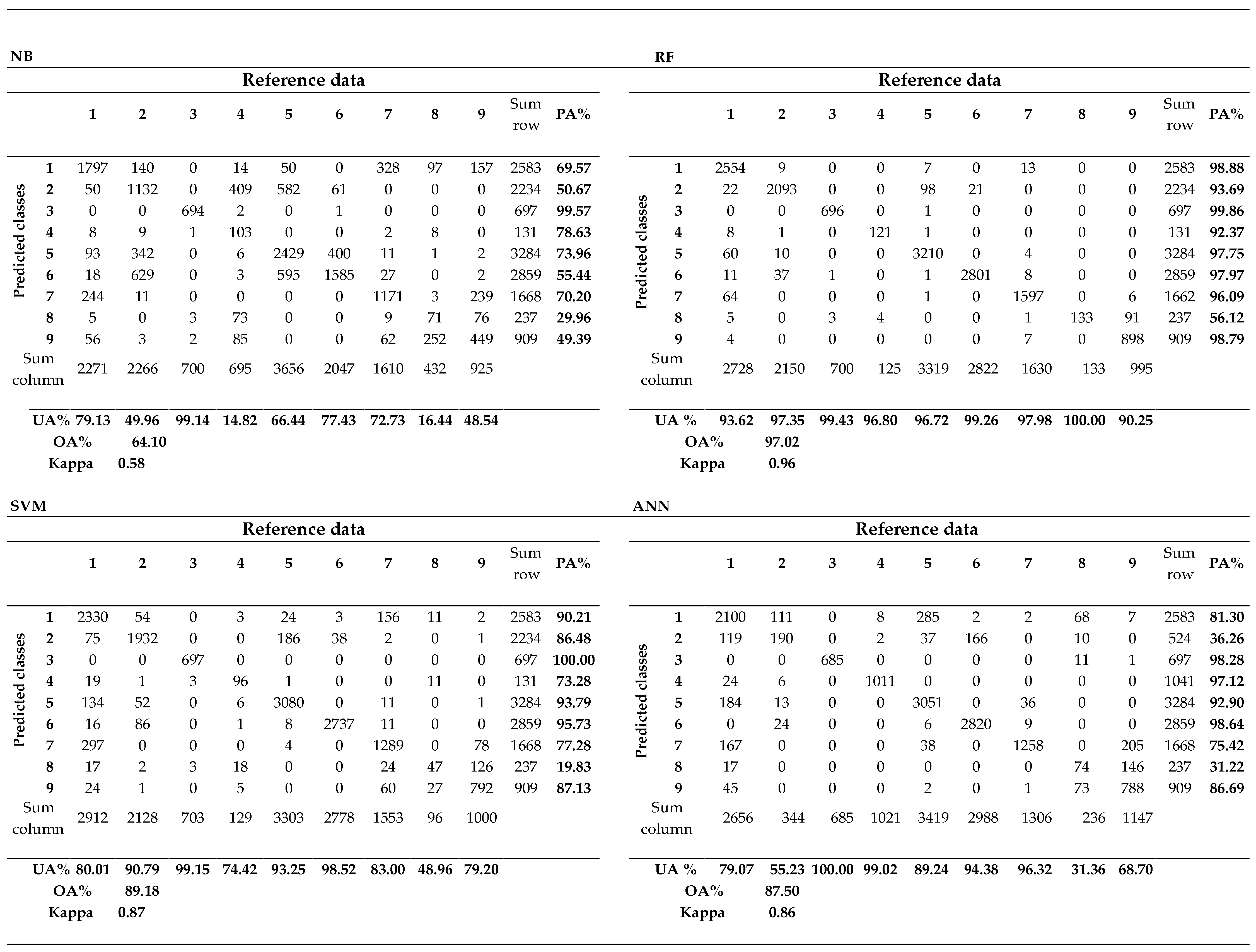
3.2. Comparison of the Mapping Accuracy of Machine Learning Algorithms

The accuracy matrices of the models were generated using 30% of the sample size (Table 4). The matrices of the MLAs (Figure 7) provide the statistical report on the agreement between reality on the ground and the maps produced. The OA, Kappa, UA, and PA algorithms were used to assess the accuracy of the models. According to the confusion matrix reports, the OA and Kappa were 64.38% and 0.58 for NB, 97.02% and 0.96 for RF, 89.74% and 0.88 for SVM, and 87% and 0.86 for ANN, respectively. The overall performance of the models was generated from the accuracy of the individual classes.

The classification accuracy for the land use classes varies significantly across the four MLAs, as presented in Figure 7. RF and SVM have effectively classified the built-up class at thresholds of >85.60% for both UA and PA. The NB model struggled to separate the built-up and mining classes. Hence, there is observable swapping between the two classes. Similarly, the ANN model showed a high commission of mining pixels to the built-up class. Thus, NB only achieved 48.54% and 49.39% for UA and PA for the built-up class, respectively. NB tends to confuse cropland with plantations. In contrast, RF, SVM, and ANN successfully extracted the cropland pixels with high metric percentages (Figure 7). All the MLAs delineated the surface water, plantation, forest, and barren classes with fairly high confidence, except for the NB model that commissioned some natural forest pixels to the plantations class.

It is worth reporting that only the RF model provided meaningful results for mapping uMngeni River catchment classes with a small area extent, which includes the barren, mining, and wetland classes. The SVM model experienced an error in omission regarding mining and wetland pixels. In contrast, the ANN model mapped the mining and wetlands classes with observable overfitting, which highly correlates with the decline in the built-up, grassland, and forest classes (Figure 5). NB significantly overfitted the barren and wetland classes at the expense of cropland and plantation land cover classes. Consequently, these accuracy metrics form the basis of the overall classification performance of each model.

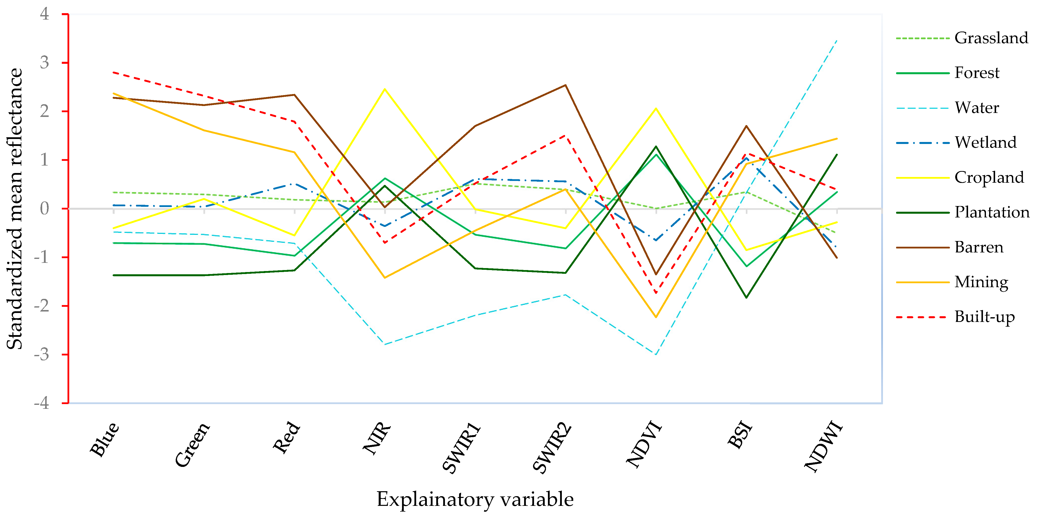
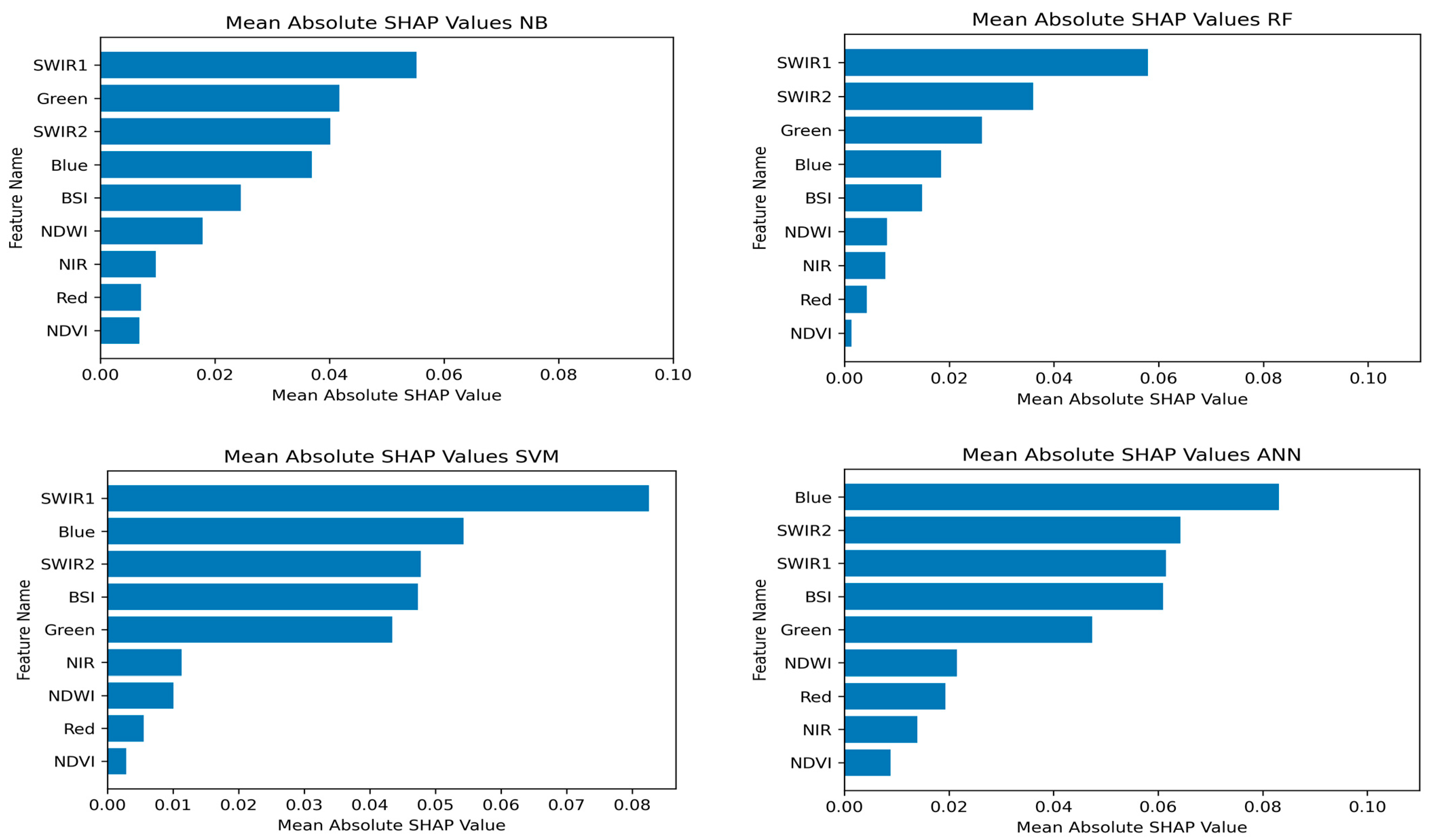
3.3. Model Feature Importance

Land cover classes were mapped through the contribution of L8-OLI multispectral bands and derived indices (Figure 2 and Figure 3). The impact of each input feature on the labeling of the classes was analysed based on the average SHAP absolute value. Figure 8 shows the feature importance bar in the degressive arrangement. Each bar represents the sum of the average SHAP values of classes per feature. In the y-axis, the longer the bar, the higher the importance of the feature, and the x-axis represents the average SHAP values for each feature.

In Figure 8, the model’s interpretation graphs depict the two common patterns across four models. The top four contributors include SWIR (B6 and B7), Blue (B2), and Green (B3) bands, and the second half shows the gradual decreasing mean SHAP value trend from BSI, NDWI, Red (B4), and NDVI. Given that our study area is dominated by vegetation land use classes, this explains why the highly ranked features are sensitive to vegetation. Thus, SWIR bands were ranked as the most important feature in overall. They are centered at 1.56–2.29 μm, allowing the detection of water content among vegetation class members [67]. Similar results have been reported in studies based on assessing Landsat features for mapping vegetation foliage, such as [68,69]. This has also been observed in other studies that used different sensors (Sentinel-2) and found that SWIR has dominance over the other features [70,71,72].

4. Discussion

The mapping of the nine land use classes in GEE was accomplished by complementing the four non-parametric MLAs (NB, RF, SVM, and ANN) to examine the LULC’s current state and the geographic distribution of each class in the uMngeni River basin. The results of this analysis will be useful in determining which planning instruments are best for protecting freshwater resources. It also sheds light on how MLAs are applied and how well they may explain the LULC in the region of undulating terrain.

Thematic land use classes were classified based on the use of the multi-spectral bands from L8-OLI imagery. It is imperative to underscore the variations in area coverage for land cover classes amongst the MLAs (Figure 6); these results align with comparative research [17,18,73] that examined machine learning classifiers in mapping LULC classes. This reflects the variability in the inherent design of the machine learning models [73,74] and the dimensionality of the data to be processed [46]. Thus, results from the RF model were used in the discussion of this work as it was the best-performing classifier.

The grassland class was identified as the most dominant class. It is widely distributed, with an area extent of 40.99% of the total catchment area. Namugize et al. [8] reported similar findings. The grassland class holds the topsoil together, increasing the water infiltration rate [75]. Therefore, it has a significant impact on groundwater recharge and water quality.

The forest provides similar ecological functions as the grassland; with an average coverage of 23.85% of the catchment area, the forest is the second largest class after grassland. It is found in abundance in the central sections and in somewhat dispersed patches in the upper and lower regions. Most notably, it mitigates climate change and acts as a carbon sink, hence preventing the deterioration of water quality [6,76]. As a result, efforts to preserve the current natural plant cover should be undertaken, and as suggested by [6,77,78], actions aimed at increasing the area covered by these classes may be encouraged.

The cropland is the fifth largest class, accounting for 10.06% of the study area. Although it is evenly dispersed throughout the catchment, homogeneous patches are observed in the northeast and stretch towards the tip of the western regions (Figure 5). Adjacent to cropland in the further north, about 9.92% of the plantation area cover was observed. The areas dominated by croplands and plantations are known for having low water quality [8,79] due to the inputs used to enhance plant life. The residuals remain in the soil and are eventually channelled to the waterbodies, impacting the freshwater ecosystem [78,79]. In light of these environmental risks, water resource managers must ensure that control measures are in place to promote sustainable agriculture and forestry.

Among the classes that account for the bigger share of the catchment area, the built-up class is the last at 10.27%. It is mostly concentrated in the southern and lower areas of the catchment. Driven by societal needs [7,8,76], it comprises a range of infrastructure types, as explained in Table 1. The built-up class creates impermeable surfaces with low water infiltration, raising water run-off [80], hiking the non-point pollutants to the rivers [8,63,79,81] and ultimately increasing the stream rate flow [82] with implications for water quality and hydrological structures. For such reasons, practical measures to control urban sprawling must be developed, as numerous studies have suggested [76,83].

Similar to built-up areas, barren areas and mining pose a hazard to freshwater resources; they occupy comparatively minor portions of the watershed, at 3.03% and 0.08%, respectively (Table 6). Water turbidity is caused by barren areas, which permit dirt particles to splash into waterbodies [84]. The mining spots are somewhat randomly dispersed along the catchment’s forest banks. Their by-products endanger human health as well as aquatic biodiversity [63]. In order to minimize the influence on waterbodies, it is advised that mining developments and barren areas within the catchment be constantly monitored and subject to management measures.

Water and wetland classes cover 1.69% and 0.12% of the study area, respectively. The wetlands are found in the north-west periphery and similar findings were also reported by [85]. Both water and wetlands are the major role players in ensuring the health of the ecosystem in general [86]. Therefore, to guarantee the continuity of their service, initiatives aimed at water harvesting and natural restoration systems should be established, as recommended by [80].

The quantitative analysis of the LULC in the catchment unpacked the underlying data regarding the LULC distribution status. These data will serve as a reference for freshwater resource managers and environmental health specialists in developing management plans and policies for freshwater resources based on informed decisions.

Since various models yield different results in different classes, it is imperative to evaluate the MLAs’ performance at the class level [29]. In light of this, only the ANN model confidently delineated the river paths (Figure 5h). However, it could not detect small dams and ponds. In contrast, RF, SVM, and NB struggled to distinguish between river trails and built-up areas (Figure 5b,d,f). This has been reported in prior studies that used pixel-based methods in LULC mapping [7,17,87] and linked them to spectral overlap between built-up areas and riverbeds or river rocks. A strong ability to map small waterbodies was demonstrated by the RF and SVM models. Similar results have been reported by [65], highlighting SVM’s efficiency in mapping small waterbodies. However, it performed poorly in defining mining pits. On the other hand, NB and ANN showed bidirectional misclassification between the built-up and mining classes. These findings are in line with [46,56]. However, RF succeeded in separating these classes with a high user accuracy score. Similar results have been reported [28,54,56], claiming that RF possesses a strong generalization technique for LULC analysis, making it less sensitive to the small variations in input vector data.

It is also worth reporting that all MLAs except the RF model struggled to delineate the wetland areas. NB and ANN tended to overfit the wetland class, while SVM commissioned some of the wetland pixels to grassland. These findings were observed in other studies [19], suggesting that this can be associated with composite signatures from the mixed pixels caused by the L8-OLI’s 30 m resolution [88], with small samples being allocated to the wetland class due to their small size. The ability to compile the MLAs’ overall performance is made possible by the precise evaluation at the class level.

Overall, all the models performed well and produced more realistic LULC maps that resemble the reality on the ground. The findings of this study indicate that RF outperformed all the MLAs with slightly higher OA and Kappa values than those recorded by the SVM model as the second-best classifier, yielding more accurate results than ANN and NB. Previous studies [9,16,17,73] have debated the comparison of RF and SVM and concluded that RF is resilient in classifying complex LULC classes. Its success is credited to its insensitivity to sample size and the advantage of the random multi-decision trees in generalization which are immune to outliers. In contrast, other studies found SVM to be superior to RF; for example, [6] found that SVM outperformed the RF model in mapping natural forest cover classes, indicating that the model’s success can be attributed to its default settings. Woldemariam et al. [18] evaluated MLAs for dynamic land use and found SVM to be superior to RF, crediting the model’s performance to the usage of the kernel functions to optimize the hyperplanes to find the optimum margin.

An emerging MLA in the remote sensing field, NB, was found unfit to analyse complex land use landscapes. Other researchers [28,29,46] also reported similar findings. This highlights the limitations in the inherent design of the model in dealing with high-dimensional data. The performance can also be associated with the sensitivity of the model to sample size. The NB classifier can be effective in large areas with more linear land cover patterns.

The results of our study proved the excellence of the RF model, which produced a more accurate LULC analysis of the uMngeni River catchment. These results will fill the gap in the literature by identifying the most suitable MLA for quantitative analysis of dimensional LULC in undulating watershed areas. In addition, this can be a useful tool for water resource managers and environmental health stakeholders to facilitate the development of freshwater resource management strategies by unpacking visual and qualitative LULC information for watershed areas.

L8-OLI multi-spectral bands with integrated indices provided good results. SWIR (1 and 2) emerged as the most influential band in the delineation of LULC classes, as discussed in Section 3.3. For such reasons, L8-OLI data were found to be reliable for analysis of the complex LULC in the undulating landscape of the catchment areas. However, it was found to be challenging to classify the pixels at the edges of the big parcels of classes and built-up class members in the core of barren and/or grassland classes or areas partially masked by trees. These findings are consistent with [19], who found that pixels in the transition zone between two parcels have been misclassified due to mixed-pixel composite signatures, as explained by [88,89]. It is challenging to discriminate smaller classes from others in L8-OLI 30 m resolution images due to mixed pixels [17]. Other studies factored in the limitations of pixel-based algorithms [24,87], associating mixed-pixel effects with the restrictions of pixel-based models to go beyond the pixel level.

5. Conclusions

The production of LULC thematic maps based on moderate-resolution satellite data is commonly used in various land cover mapping studies. Using such data gives environmental managers the timely quantitative spatial information they need to implement best practices for natural resource conservation. In this study, four pixel-based non-parametric MLAs, NB, RF, SVM, and ANN, were attested in the classification of thematic LULC classes in the uMngeni River Catchment landscape, South Africa. Moderate-resolution (30 m) data from the L8-OLI sensor were harnessed for mapping nine identified LULC classes. The referenced data acquired from field surveys and Google Earth Pro high-resolution imagery were used for both training models and accuracy assessment. The findings of this study demonstrated the disparities in the MLAs’ performances at the class level, resulting in variations in LULC class area coverage across four MLAs. Overall, the RF model outperformed all other models, producing a map that closely resembles the reality on the ground with 97.02% overall accuracy and a kappa value of 0.96, which are in line with a number of studies on mapping LULC in the catchment areas. We discovered that the ANN model performed well in defining the river trails compared to other models, while RF proved to be efficient in mapping classes with tiny area sizes. When viewed from the viewpoint of other models, SVM tends to experience the commission of mining class members to built-up classes, hence producing low accuracies in the mining class. As evidenced by their low accuracies, NB and ANN either overfitted or underestimated the LULC classes covering a small area. These errors stem from two directions: first, the variations in the designs of the models hinder them from analysing the data at the subpixel level; second, the 30 m resolution data used makes it difficult for MLA models to classify the impure Landsat pixels due to low resolution. The findings of this work will demonstrate the practical application of MLAs in mapping LULC and serve as an anchor for water resource managers and other relevant environmental health professionals to update or establish the policies and management plans aimed at conserving water resources based on informed decisions. In addition, using RF for classification, with balanced hyperparameter tuning and Landsat data as used in this study, proved to be efficient in mapping LULC in the Umngeni River Catchment. As a result, the method used in this study can be adapted to other research in similar geographic settings.

References

1. Mekuria, W.; Gedle, A.; Tesfaye, Y.; Phimister, E. Implications of Changes in Land Use for Ecosystem Service Values of Two Highly Eroded Watersheds in Lake Abaya Chamo Sub-Basin, Ethiopia. Ecosyst. Serv. 2023, 64, 101564. [Google Scholar] [CrossRef]
2. Aneseyee, A.B.; Soromessa, T.; Elias, E. The Effect of Land Use/Land Cover Changes on Ecosystem Services Valuation of Winike Watershed, Omo Gibe Basin, Ethiopia. Hum. Ecol. Risk Assess. 2020, 26, 2608–2627. [Google Scholar] [CrossRef]
3. Pullanikkatil, D.; Palamuleni, L.G.; Ruhiiga, T.M. Land Use/Land Cover Change and Implications for Ecosystems Services in the Likangala River Catchment, Malawi. Phys. Chem. Earth 2016, 93, 96–103. [Google Scholar] [CrossRef]
4. Lynch, A.J.; Cooke, S.J.; Arthington, A.H.; Baigun, C.; Bossenbroek, L.; Dickens, C.; Harrison, I.; Kimirei, I.; Langhans, S.D.; Murchie, K.J.; et al. People Need Freshwater Biodiversity. Wiley Interdiscip. Rev. Water 2023, 10, e1633. [Google Scholar] [CrossRef]
5. Nyathi, N.A.; Zhao, W.; Musakwa, W. Land Use Land Cover Changes and Their Impacts on Ecosystem Services in the Nzhelele River Catchment, South Africa. ISPRS Ann. Photogramm. Remote Sens. Spat. Inf. Sci. 2020, 5, 809–816. [Google Scholar] [CrossRef]
6. Gyamfi-Ampadu, E.; Gebreslasie, M.; Mendoza-Ponce, A. Mapping Natural Forest Cover Using Satellite Imagery of Nkandla Forest Reserve, KwaZulu-Natal, South Africa. Remote Sens. Appl. 2020, 18, 100302. [Google Scholar] [CrossRef]
7. Obaid, A.; Adam, E.; Ali, K.A. Land Use and Land Cover Change in the Vaal Dam Catchment, South Africa: A Study Based on Remote Sensing and Time Series Analysis. Geomatics 2023, 3, 205–220. [Google Scholar] [CrossRef]
8. Namugize, J.N.; Jewitt, G.; Graham, M. Effects of Land Use and Land Cover Changes on Water Quality in the UMngeni River Catchment, South Africa. Phys. Chem. Earth 2018, 105, 247–264. [Google Scholar] [CrossRef]
9. Ouchra, H.; Belangour, A.; Erraissi, A. Comparison of Machine Learning Methods for Satellite Image Classification: A Case Study of Casablanca Using Landsat Imagery and Google Earth Engine. J. Environ. Earth Sci. 2023, 5, 118–134. [Google Scholar] [CrossRef]
10. Akar, O.; Tunc Gormus, E. Land Use/Land Cover Mapping from Airborne Hyperspectral Images with Machine Learning Algorithms and Contextual Information. Geocarto Int. 2022, 37, 3963–3990. [Google Scholar] [CrossRef]
11. Lekka, C.; Petropoulos, G.P.; Detsikas, S.E. Appraisal of EnMAP Hyperspectral Imagery Use in LULC Mapping When Combined with Machine Learning Pixel-Based Classifiers. Environ. Model. Softw. 2024, 173, 105956. [Google Scholar] [CrossRef]
12. Delogu, G.; Caputi, E.; Perretta, M.; Ripa, M.N.; Boccia, L. Using PRISMA Hyperspectral Data for Land Cover Classification with Artificial Intelligence Support. Sustainability 2023, 15, 13786. [Google Scholar] [CrossRef]
13. James, D.; Collin, A.; Mury, A.; Costa, S. Very High Resolution Land Use and Land Cover Mapping Using Pleiades-1 Stereo Imagery and Machine Learning. Int. Arch. Photogramm. Remote Sens. Spat. Inf. Sci. 2020, XLIII-B2-2020, 675–682. [Google Scholar] [CrossRef]
14. Mahmoud, R.; Hassanin, M.; Al Feel, H.; Badry, R.M. Machine Learning-Based Land Use and Land Cover Mapping Using Multi-Spectral Satellite Imagery: A Case Study in Egypt. Sustainability 2023, 15, 9467. [Google Scholar] [CrossRef]
15. Bayas, S.; Sawant, S.; Dhondge, I.; Kankal, P.; Joshi, A. Land Use Land Cover Classification Using Different ML Algorithms on Sentinel-2 Imagery. In Advanced Machine Intelligence and Signal Processing; Springer: Singapore, 2022; pp. 761–777. [Google Scholar]
16. Parashar, D.; Kumar, A.; Palni, S.; Pandey, A.; Singh, A.; Singh, A.P. Use of Machine Learning-Based Classification Algorithms in the Monitoring of Land Use and Land Cover Practices in a Hilly Terrain. Environ. Monit. Assess. 2024, 196, 8. [Google Scholar] [CrossRef]
17. Loukika, K.N.; Keesara, V.R.; Sridhar, V. Analysis of Land Use and Land Cover Using Machine Learning Algorithms on Google Earth Engine for Munneru River Basin, India. Sustainability 2021, 13, 13758. [Google Scholar] [CrossRef]
18. Woldemariam, G.W.; Tibebe, D.; Mengesha, T.E.; Gelete, T.B. Machine-Learning Algorithms for Land Use Dynamics in Lake Haramaya Watershed, Ethiopia. Model Earth Syst. Environ. 2022, 8, 3719–3736. [Google Scholar] [CrossRef]
19. Dash, P.; Sanders, S.L.; Parajuli, P.; Ouyang, Y. Improving the Accuracy of Land Use and Land Cover Classification of Landsat Data in an Agricultural Watershed. Remote Sens. 2023, 15, 4020. [Google Scholar] [CrossRef]
20. Hughes, C.J.; De Winnaar, G.; Schulze, R.E.; Mander, M.; Jewitt, G.P.W. Mapping of Water-Related Ecosystem Services in the UMngeni Catchment Using a Daily Time-Step Hydrological Model for Prioritisation of Ecological Infrastructure Investment—Part 2: Outputs. Water SA 2018, 44, 590–600. [Google Scholar] [CrossRef]
21. Kusangaya, S.; Warburton, M.; Archer van Garderen, E. Use of ACRU, a Distributed Hydrological Model, to Evaluate How Errors from Downscaled Rainfall Are Propagated in Simulated Runoff in UMngeni Catchment, South Africa. Hydrol. Sci. J. 2017, 62, 1995–2011. [Google Scholar] [CrossRef]
22. Kaur, H.; Tyagi, S.; Mehta, M.; Singh, D. Time Series (2001/2002–2021) Analysis of Earth Observation Data Using Google Earth Engine (GEE) for Detecting Changes in Land Use Land Cover (LULC) with Specific Reference to Forest Cover in East Godavari Region, Andhra Pradesh, India. J. Earth Syst. Sci. 2023, 132, 86. [Google Scholar] [CrossRef]
23. Mandal, S.; Bandyopadhyay, A.; Bhadra, A. Dynamics and Future Prediction of LULC on Pare River Basin of Arunachal Pradesh Using Machine Learning Techniques. Environ. Monit Assess 2023, 195, 709. [Google Scholar] [CrossRef]
24. Maviza, A.; Ahmed, F. Analysis of Past and Future Multi-Temporal Land Use and Land Cover Changes in the Semi-Arid Upper-Mzingwane Sub-Catchment in the Matabeleland South Province of Zimbabwe. Int. J. Remote Sens. 2020, 41, 5206–5227. [Google Scholar] [CrossRef]
25. Foga, S.; Scaramuzza, P.L.; Guo, S.; Zhu, Z.; Dilley, R.D.; Beckmann, T.; Schmidt, G.L.; Dwyer, J.L.; Joseph Hughes, M.; Laue, B. Cloud Detection Algorithm Comparison and Validation for Operational Landsat Data Products. Remote Sens. Environ. 2017, 194, 379–390. [Google Scholar] [CrossRef]
26. Mashala, M.J.; Dube, T.; Ayisi, K.K.; Ramudzuli, M.R. Using the Google Earth Engine Cloud-Computing Platform to Assess the Long-Term Spatial Temporal Dynamics of Land Use and Land Cover within the Letaba Watershed, South Africa. Geocarto Int. 2023, 38, 2252781. [Google Scholar] [CrossRef]
27. Floreano, I.X.; de Moraes, L.A.F. Land Use/Land Cover (LULC) Analysis (2009–2019) with Google Earth Engine and 2030 Prediction Using Markov-CA in the Rondônia State, Brazil. Environ. Monit. Assess. 2021, 193, 239. [Google Scholar] [CrossRef]
28. Orieschnig, C.A.; Belaud, G.; Venot, J.-P.; Massuel, S.; Ogilvie, A. Input Imagery, Classifiers, and Cloud Computing: Insights from Multi-Temporal LULC Mapping in the Cambodian Mekong Delta. Eur. J. Remote Sens. 2021, 54, 398–416. [Google Scholar] [CrossRef]
29. Palanisamy, P.A.; Jain, K.; Bonafoni, S. Machine Learning Classifier Evaluation for Different Input Combinations: A Case Study with Landsat 9 and Sentinel-2 Data. Remote Sens. 2023, 15, 3241. [Google Scholar] [CrossRef]
30. Viana, C.M.; Girão, I.; Rocha, J. Long-Term Satellite Image Time-Series for Land Use/Land Cover Change Detection Using Refined Open Source Data in a Rural Region. Remote Sens. 2019, 11, 1104. [Google Scholar] [CrossRef]
31. Gao, B.C. NDWI—A Normalized Difference Water Index for Remote Sensing of Vegetation Liquid Water from Space. Remote Sens. Environ. 1996, 58, 257–266. [Google Scholar] [CrossRef]
32. Nguyen, C.T.; Chidthaisong, A.; Kieu Diem, P.; Huo, L.-Z. A Modified Bare Soil Index to Identify Bare Land Features during Agricultural Fallow-Period in Southeast Asia Using Landsat 8. Land 2021, 10, 231. [Google Scholar] [CrossRef]
33. Rouse, J.W.; Haas, R.H.; Schell, J.A.; Deering, D.W. Monitoring vegetation systems in the great plains with ERTS. In Proceedings of the Third NASA Earth Resources Technology Satellite Symposium, Washington, DC, USA, 10–14 December 1973; pp. 309–317. [Google Scholar]
34. Rikimaru, A.; Roy, P.S.; Miyatake, S. Tropical Forest Cover Density Mapping. Trop. Ecol. 2002, 43, 39–47. [Google Scholar]
35. Carlotto, M.J. Effect of Errors in Ground Truth on Classification Accuracy. Int. J. Remote Sens. 2009, 30, 4831–4849. [Google Scholar] [CrossRef]
36. Foody, G.M. Assessing the Accuracy of Land Cover Change with Imperfect Ground Reference Data. Remote Sens. Environ. 2010, 114, 2271–2285. [Google Scholar] [CrossRef]
37. Olofsson, P.; Foody, G.M.; Herold, M.; Stehman, S.V.; Woodcock, C.E.; Wulder, M.A. Good Practices for Estimating Area and Assessing Accuracy of Land Change. Remote Sens. Environ. 2014, 148, 42–57. [Google Scholar] [CrossRef]
38. Gandhi, Ujaval, 2021. End-to-End Google Earth Engine Course. Spatial Thoughts. Available online: https://courses.spatialthoughts.com/end-to-end-gee.html (accessed on 2 February 2024).
39. Gyamfi-Ampadu, E.; Gebreslasie, M.; Mendoza-Ponce, A. Evaluating Multi-sensors Spectral and Spatial Resolutions for Tree Species Diversity Prediction. Remote Sens. 2021, 13, 1033. [Google Scholar] [CrossRef]
40. Costache, R.; Tin, T.T.; Arabameri, A.; Crăciun, A.; Costache, I.; Islam, A.R.M.T.; Sahana, M.; Pham, B.T. Stacking State-of-the-Art Ensemble for Flash-Flood Potential Assessment. Geocarto Int. 2022, 37, 13812–13838. [Google Scholar] [CrossRef]
41. Breiman, L.E.O. Random Forests. Mach. Learn. 2001, 45, 5–32. [Google Scholar] [CrossRef]
42. Zhang, Q.; Liu, M.; Zhang, Y.; Mao, D.; Li, F.; Wu, F.; Song, J.; Li, X.; Kou, C.; Li, C.; et al. Comparison of Machine Learning Methods for Predicting Soil Total Nitrogen Content Using Landsat-8, Sentinel-1, and Sentinel-2 Images. Remote Sens. 2023, 15, 2907. [Google Scholar] [CrossRef]
43. Mather, P.M.; Koch, M. Computer Processing of Remotely-Sensed Images: An Introduction; John Wiley & Sons: Hoboken, NJ, USA, 2011; ISBN 1119956404. [Google Scholar]
44. Cuypers, S.; Nascetti, A.; Vergauwen, M. Land Use and Land Cover Mapping with VHR and Multi-Temporal Sentinel-2 Imagery. Remote Sens. 2023, 15, 2501. [Google Scholar] [CrossRef]
45. Kim, Y.H.; Im, J.; Ha, H.K.; Choi, J.K.; Ha, S. Machine Learning Approaches to Coastal Water Quality Monitoring Using GOCI Satellite Data. GIsci Remote Sens. 2014, 51, 158–174. [Google Scholar] [CrossRef]
46. Camargo, F.F.; Sano, E.E.; Almeida, C.M.; Mura, J.C.; Almeida, T. A Comparative Assessment of Machine-Learning Techniques for Land Use and Land Cover Classification of the Brazilian Tropical Savanna Using ALOS-2/PALSAR-2 Polarimetric Images. Remote Sens. 2019, 11, 1600. [Google Scholar] [CrossRef]
47. Yulianto, F.; Raharjo, P.D.; Pramono, I.B.; Setiawan, M.A.; Chulafak, G.A.; Nugroho, G.; Sakti, A.D.; Nugroho, S.; Budhiman, S. Prediction and Mapping of Land Degradation in the Batanghari Watershed, Sumatra, Indonesia: Utilizing Multi-Source Geospatial Data and Machine Learning Modeling Techniques. Model Earth Syst. Environ. 2023, 9, 4383–4404. [Google Scholar] [CrossRef]
48. Huang, C.; Davis, L.S.; Townshend, J.R.G. An Assessment of Support Vector Machines for Land Cover Classification. Int. J. Remote Sens. 2002, 23, 725–749. [Google Scholar] [CrossRef]
49. Lantzanakis, G.; Mitraka, Z.; Chrysoulakis, N. X-SVM: An Extension of C-SVM Algorithm for Classification of High-Resolution Satellite Imagery. IEEE Trans. Geosci. Remote Sens. 2021, 59, 3805–3815. [Google Scholar] [CrossRef]
50. Srivastava, P.K.; Han, D.; Rico-Ramirez, M.A.; Bray, M.; Islam, T. Selection of Classification Techniques for Land Use/Land Cover Change Investigation. Adv. Space Res. 2012, 50, 1250–1265. [Google Scholar] [CrossRef]
51. Martins, S.; Bernardo, N.; Ogashawara, I.; Alcantara, E. Support Vector Machine Algorithm Optimal Parameterization for Change Detection Mapping in Funil Hydroelectric Reservoir (Rio de Janeiro State, Brazil). Model Earth Syst. Environ. 2016, 2, 138. [Google Scholar] [CrossRef]
52. Roushangar, K.; Aalami, M.T.; Golmohammadi, H.; Shahnazi, S. Monitoring and Prediction of Land Use/Land Cover Changes and Water Requirements in the Basin of the Urmia Lake, Iran. Water Supply 2023, 23, 2299–2312. [Google Scholar] [CrossRef]
53. Saraf, N.M.; Lokman, M.F.; Abdul Rasam, A.R.; Hashim, N. Assessment of Urban Growth Changes in Klang District Using Support Vector Machine by Different Kernel. IOP Conf Ser Earth Environ. Sci 2022, 1051, 012023. [Google Scholar] [CrossRef]
54. Dahiya, N.; Gupta, S.; Singh, S. Qualitative and Quantitative Analysis of Artificial Neural Network-Based Post-Classification Comparison to Detect the Earth Surface Variations Using Hyperspectral and Multispectral Datasets. J. Appl. Remote Sens. 2023, 17, 032403. [Google Scholar] [CrossRef]
55. Wu, J.L.; Ho, C.R.; Huang, C.C.; Srivastav, A.L.; Tzeng, J.H.; Lin, Y.T. Hyperspectral Sensing for Turbid Water Quality Monitoring in Freshwater Rivers: Empirical Relationship between Reflectance and Turbidity and Total Solids. Sensors 2014, 14, 22670–22688. [Google Scholar] [CrossRef]
56. Chen, H.; Lin, X.; Sun, Y.; Wen, J.; Wu, X.; You, D.; Cheng, J.; Zhang, Z.; Zhang, Z.; Wu, C.; et al. Performance Assessment of Four Data-Driven Machine Learning Models: A Case to Generate Sentinel-2 Albedo at 10 Meters. Remote Sens. 2023, 15, 2684. [Google Scholar] [CrossRef]
57. Deshpande, A.R.; Emmanuel, M. Context Based Recommendation Methods: A Brief Review. Presented at Conference on Cognitive Knowledge Engineering, Aurangabad, Maharashtra, India, 2016; pp. 14–19. Available online: https://www.researchgate.net/profile/Ratnadeep-Deshmukh-2/publication/329059854_2nd_International_Conference_on_Knowledge_Engineering/links/5bf3dcdba6fdcc3a8de38181/2nd-International-Conference-on-Knowledge-Engineering.pdf#page=58 (accessed on 30 March 2024).
58. Hafeez, S.; Wong, M.S.; Ho, H.C.; Nazeer, M.; Nichol, J.; Abbas, S.; Tang, D.; Lee, K.H.; Pun, L. Comparison of Machine Learning Algorithms for Retrieval of Water Quality Indicators in Case-Ii Waters: A Case Study of Hong Kong. Remote Sens. 2019, 11, 617. [Google Scholar] [CrossRef]
59. Lundberg, S.M.; Allen, P.G.; Lee, S.-I. A Unified Approach to Interpreting Model Predictions. Adv. Neural Inf. Process. Syst. 2017, 30. Available online: https://github.com/slundberg/shap (accessed on 23 May 2024).
60. Wei, P.; Lu, Z.; Song, J. Variable importance analysis: A comprehensive review. Reliab. Eng. Syst. Saf. 2015, 142, 399–432. [Google Scholar] [CrossRef]
61. Hosseiny, B.; Abdi, A.M.; Jamali, S. Urban land use and land cover classification with interpretable machine learning—A case study using Sentinel-2 and auxiliary data. Remote Sens. Appl. Soc. Environ. 2022, 28, 100843. [Google Scholar] [CrossRef]
62. Yilmaz, E.O.; Kavzoglu, T. Classification of jilin-1 gp01 hyperspectral image using machine learning techniques with explainable artificial intelligence. Intercont. Geoinf. Days 2022, 5, 145–148. [Google Scholar]
63. Hua, A.K. Land Use Land Cover Changes in Detection of Water Quality: A Study Based on Remote Sensing and Multivariate Statistics. J. Environ. Public Health 2017, 2017, 5–7. [Google Scholar] [CrossRef]
64. Congalton, R.G. A Review of Assessing the Accuracy of Classifications of Remotely Sensed Data. Remote Sens. Environ. 1991, 37, 35–46. [Google Scholar] [CrossRef]
65. Kang, C.S.; Kanniah, K.D.; Mohd Najib, N.E. Google Earth Engine for Landsat Image Processing and Monitoring Land Use/Land Cover Changes in the Johor River Basin, Malaysia. In Proceedings of the International Geoscience and Remote Sensing Symposium (IGARSS), Brussels, Belgium, 11–16 July 2021; pp. 4236–4239. [Google Scholar]
66. Story, M.; Congalton, R.G. Accuracy Assessment: A User’s Perspective. Photogramm. Eng. Remote Sens. 1986, 52, 397–399. [Google Scholar]
67. Lukeš, P.; Stenberg, P.; Rautiainen, M.; Mõttus, M.; Vanhatalo, K.M. Optical Properties of Leaves and Needles for Boreal Tree Species in Europe. Remote Sens. Lett. 2013, 4, 667–676. [Google Scholar] [CrossRef]
68. Schultz, B.; Immitzer, M.; Formaggio, A.; Sanches, I.; Luiz, A.; Atzberger, C. Self-Guided Segmentation and Classification of Multi-Temporal Landsat 8 Images for Crop Type Mapping in Southeastern Brazil. Remote Sens. 2015, 7, 14482–14508. [Google Scholar] [CrossRef]
69. Sothe, C.; Almeida, C.; Liesenberg, V.; Schimalski, M. Evaluating Sentinel-2 and Landsat-8 Data to Map Sucessional Forest Stages in a Subtropical Forest in Southern Brazil. Remote Sens. 2017, 9, 838. [Google Scholar] [CrossRef]
70. Chen, H.; Yang, L.; Wu, Q. Enhancing Land Cover Mapping and Monitoring: An Interactive and Explainable Machine Learning Approach Using Google Earth Engine. Remote Sens. 2023, 15, 4585. [Google Scholar] [CrossRef]
71. McCarty, D.A.; Kim, H.W.; Lee, H.K. Evaluation of Light Gradient Boosted Machine Learning Technique in Large Scale Land Use and Land Cover Classification. Environments 2020, 7, 84. [Google Scholar] [CrossRef]
72. Abdi, A.M. Land Cover and Land Use Classification Performance of Machine Learning Algorithms in a Boreal Landscape Using Sentinel-2 Data. GIsci Remote Sens. 2020, 57, 1–20. [Google Scholar] [CrossRef]
73. Ashiagbor, G.; Asare-Ansah, A.O.; Amoah, E.B.; Asante, W.A.; Mensah, Y.A. Assessment of Machine Learning Classifiers in Mapping the Cocoa-Forest Mosaic Landscape of Ghana. Sci. Afr. 2023, 20, e01718. [Google Scholar] [CrossRef]
74. Foody, G.M. Valuing Map Validation: The Need for Rigorous Land Cover Map Accuracy Assessment in Economic Valuations of Ecosystem Services. Ecol. Econ. 2015, 111, 23–28. [Google Scholar] [CrossRef]
75. Machado, R.A.S.; Oliveira, A.G.; Lois-González, R.C. Urban Ecological Infrastructure: The Importance of Vegetation Cover in the Control of Floods and Landslides in Salvador/Bahia, Brazil. Land Use Policy 2019, 89, 104180. [Google Scholar] [CrossRef]
76. Abbas, H.; Tao, W.; Khan, G.; Alrefaei, A.F.; Iqbal, J.; Albeshr, M.F.; Kulsoom, I. Multilayer Perceptron and Markov Chain Analysis Based Hybrid-Approach for Predicting Land Use Land Cover Change Dynamics with Sentinel-2 Imagery. Geocarto Int. 2023, 38, 2256297. [Google Scholar] [CrossRef]
77. Gyamfi-Ampadu, E.; Gebreslasie, M.; Mendoza-Ponce, A. Multi-Decadal Spatial and Temporal Forest Cover Change Analysis of Nkandla Natural Reserve, South Africa. J. Sustain. For. 2022, 41, 959–982. [Google Scholar] [CrossRef]
78. du Plessis, A.; Harmse, T.; Ahmed, F. Quantifying and Predicting the Water Quality Associated with Land Cover Change: A Case Study of the Blesbok Spruit Catchment, South Africa. Electron. J. Theor. Phys. 2014, 11, 2946–2968. [Google Scholar] [CrossRef]
79. Mararakanye, N.; Le Roux, J.J.; Franke, A.C. Long-Term Water Quality Assessments under Changing Land Use in a Large Semi-Arid Catchment in South Africa. Sci. Total Environ. 2022, 818, 151670. [Google Scholar] [CrossRef]
80. Schütte, S.; Schulze, R.E. Projected Impacts of Urbanisation on Hydrological Resource Flows: A Case Study within the UMngeni Catchment, South Africa. J. Environ. Manag. 2017, 196, 527–543. [Google Scholar] [CrossRef]
81. Kibena, J.; Nhapi, I.; Gumindoga, W. Assessing the Relationship between Water Quality Parameters and Changes in Landuse Patterns in the Upper Manyame River, Zimbabwe. Phys. Chem. Earth 2014, 67–69, 153–163. [Google Scholar] [CrossRef]
82. Tena, T.M.; Mwaanga, P.; Nguvulu, A. Impact of Land Use/Land Cover Change on Hydrological Components in Chongwe River Catchment. Sustainability 2019, 11, 6415. [Google Scholar] [CrossRef]
83. Jewitt, D.; Goodman, P.S.; Erasmus, B.F.N.; O’Connor, T.G.; Witkowski, E.T.F. Systematic Land-Cover Change in KwaZulu-Natal, South Africa: Implications for Biodiversity. S. Afr. J. Sci. 2015, 111, 9. [Google Scholar] [CrossRef]
84. Twesigye, C.K. The Impact of Land Use Activities on Vegetation Cover and Water Quality in the Lake Victoria Watershed. Open Environ. Eng. J. 2011, 4, 66–77. [Google Scholar] [CrossRef]
85. Moodley, K.; Toucher, M.L.; Lottering, R.T. Simulating Future Land-Use within the UThukela and UMngeni Catchments in KwaZulu-Natal. Sci. Afr. 2023, 20, e01666. [Google Scholar] [CrossRef]
86. Balha, A.; Mallick, J.; Pandey, S.; Gupta, S.; Singh, C.K. A Comparative Analysis of Different Pixel and Object-Based Classification Algorithms Using Multi-Source High Spatial Resolution Satellite Data for LULC Mapping. Earth Sci. Inform. 2021, 14, 2231–2247. [Google Scholar] [CrossRef]
87. Nayak, A.; Bhushan, B. Wetland Ecosystems and Their Relevance to the Environment. In Handbook of Research on Monitoring and Evaluating the Ecological Health of Wetlands; IGI Global: Hershey, PA, USA, 2022; pp. 1–16. [Google Scholar]
88. Campbell, J.B.; Wynne, R.H. Introduction to Remote Sensing; Guilford Press: New York, NY, USA, 2011; ISBN 1609181778. [Google Scholar]
89. Lillesand, T.; Kiefer, R.W.; Chipman, J. Remote Sensing and Image Interpretation; John Wiley & Sons: Hoboken, NJ, USA, 2015; ISBN 111834328X. [Google Scholar]
Figure 1. The conceptual framework of the study.
Remotesensing 16 02219 g001
Figure 2. Layout of the uMngeni River catchment with elevation gradients, the river network, and dams.
Remotesensing 16 02219 g002
Figure 3. The variable collinearity heatmap. Blue to red shows an increasing correlation relationship and vice versa.
Remotesensing 16 02219 g003
Figure 4. Standardized average reflectance values of each land use class.
Remotesensing 16 02219 g004
Figure 5. UMngeni River catchment LULC maps produced by NB, RF, SVM, and ANN models with detailed small portions in (ah).
Remotesensing 16 02219 g005
Figure 6. The spatial distribution of land use classes produced by each MLA.
Remotesensing 16 02219 g006
Figure 7. Confusion matrix and accuracy metrics for NB, RF, SVM, and ANN.
Remotesensing 16 02219 g007
Figure 8. Model feature importance based on the mean absolute SHAP value.
Remotesensing 16 02219 g008