Accurate Calculation of Upper Biomass Volume of Single Trees Using Matrixial Representation of LiDAR Data

Abstract

This paper introduces a novel method for accurately calculating the upper biomass of single trees using Light Detection and Ranging (LiDAR) point cloud data. The proposed algorithm involves classifying the tree point cloud into two distinct ones: the trunk point cloud and the crown point cloud. Each part is then processed using specific techniques to create a 3D model and determine its volume. The trunk point cloud is segmented based on individual stems, each of which is further divided into slices that are modeled as cylinders. On the other hand, the crown point cloud is analyzed by calculating its footprint and gravity center. The footprint is further divided into angular sectors, with each being used to create a rotating surface around the vertical line passing through the gravity center. All models are represented in a matrix format, simplifying the process of minimizing and calculating the tree’s upper biomass, consisting of crown biomass and trunk biomass. To validate the proposed approach, both terrestrial and airborne datasets are utilized. A comparison with existing algorithms in the literature confirms the effectiveness of the new method. For a tree dimensions estimation, the study shows that the proposed algorithm achieves an average fit between 0.01 m and 0.49 m for individual trees. The maximum absolute quantitative accuracy equals 0.49 m, and the maximum relative absolute error equals 0.29%.

1. Introduction

A Light Detection and Ranging (LiDAR) system is considered to be the main data source of a Digital Surface Model (DSM) and Digital Twin (DT), which characterize virtual representations of real-world features [1]. Indeed, DSM and DT can improve the realization of thematic systems such as City Information Modeling (CIM) [2], Building Information Modeling (BIM) [3], Land Information Modeling (LIM) [4], and Tree Information Modeling (TIM) [5]. Furthermore, although the volume of LiDAR data is large, it has been popularly utilized in Geographic Information Systems (GIS), forest monitoring, and decision-making.

A tree’s biomass may be defined by the total mass of living organic matter in the tree. It is divided into aboveground biomass and belowground biomass. Calculations of the aboveground tree biomass are conducted for forest complexes [6,7,8] and individual trees [9,10], taking into account the biomass of the trunks, branches, leaves, and roots.

Accurate forest biomass estimation is essential for forestry management [10], enabling the determination of forest productivity, wood resources, and bioenergy potential. This involves monitoring changes in tree crowns and biomass quantity with respect to variations in air pollution, carbon dioxide (CO₂) levels, temperature, and precipitation [11,12,13,14]. Based on tree biomass, the absorption of carbon dioxide from the atmosphere can be calculated using indicators, like Leaf Area Index (LAI) [15,16,17,18] and other coefficients extensively described in [19].

To estimate the aboveground tree biomass (trunks, branches, and leaves) and tree parameters, such as height, crown spread, and trunk diameter at breast height, Zani et al. [20] conducted empirical destructive studies to estimate the aboveground biomass of selected five tree species (trunk, branches, and leaves) based on the height and trunk diameter at breast height. Calculations were carried out following the procedure outlined by botanists [21]. The results were positively verified with 439 felled trees. Similar destructive studies [22] were conducted with 286 felled trees to estimate the aboveground and belowground biomass of individual trees of a selected species. Based on the trunk diameter at breast height, allometric modeling [23,24] was applied to determine the parameters that allowed for the estimation of aboveground biomass.

The main research question related to determining tree biomass is based on the data collected by various forest remote sensing techniques: satellite imaging, aerial photogrammetry, spectrometer, terrestrial and airborne laser scanning (TLS/ALS), and radar [7,25]. The development of remote sensing measurement techniques, associated with increased spatial and temporal resolutions, allows for increasingly accurate forest biomass estimation [20,26,27,28]. Recent studies conducted using neural networks [29,30] allow for the differentiation of tree species [31]. Utilizing the results of remote sensing measurements, point cloud processing is performed on LiDAR measurements, creating subsets representing individual trees [25,32,33]. Subsequent 3D modeling of individual trees is carried out on these subsets. Such tree models are then used for visualizing and calculating basic geometric parameters of crowns, trunks, and branches [34,35]. Approximate determination of aboveground biomass is possible using the geometric shape of tree crowns [10]. Tree metric data facilitate the estimation of aboveground biomass [23]. Calculations are supported by soil and forest floor indicators [36]. The most accurate determinations of aboveground tree biomass are achieved using radar measurements [37,38].

Calculating a tree’s upper biomass volume represents a great challenge in the literature because the tree crown geometries are complicated. That is why most of the previously suggested approaches suffered from limitations, especially regarding the overestimation issue. In this study, the authors propose calculating tree biomass based on the 3D tree models generated by using subsets of LiDAR point clouds representing individual trees. The goal is to develop a method for 3D tree modeling that allows for accurately calculating the tree upper biomass.

1.1. Related Works

The reconstruction of 3D models of individual trees is based on ALS and TLS data [38,39,40,41,42,43], which are associated with photogrammetric and remote sensing measurements [10]. The modeling foundations are defined in the City GML 3.0 standard [44], under the Tree Information Modeling (TIM) system at various Levels of Detail (LoD) [44,45,46]. Three-dimensional modeling of the tree canopy, trunk, and branches relies on various algorithms for crown modeling [40,47,48,49] and tree skeleton modeling [43,50,51,52]. The common solutions are based on defining the shape of the canopy using geometric solids, such as cylinders, cones, and spheres (Figure 1a). These solids are fitted to different tree species with specified crown morphologies [35,46,52]. These models are based on generalized horizontal projections of the crowns and determined tree heights (Figure 1b).

More realistic 3D tree models are based on creating tree solids, often limited to the crown. Kato et al. [40] show different crown solids associated with tree species (Figure 2). They [40] modeled trees using Radial Basis Functions (RBF) and the isosurface algorithm [53].

Interesting algorithms for automatic 3D tree modeling were presented in [33]. These include the 3D concave hull algorithm, 3D alpha shape algorithm, convex hull by slices algorithm, and Voxel model (Figure 3).

The 3D concave hull algorithm allows for scaling the model [38] via adjusting its parameters (Figure 4). This way, tree hulls of various generalizations can be created depending on the radius of the nearest point search in the point cloud.

The modeled 3D tree crowns serve as the basis for calculating biomass and predicting the sizes of trunks and branches [41]. It should be noted that the tree crown is not a homogeneous structure and representing it as a solid is a significant simplification [40]. This is well illustrated in Figure 5.

Traditional methods for determining trunk volume and tree canopy use dendrometric tables. They contain data for calculating the volume of trunks and crowns of selected tree species. There are tools ready to calculate the volume by specifying the selected parameters of the tree. There are also known application solutions based on the Smalian formula, Huber’s formula, and Bruce’s formula [54]. However, these traditional methods based on tabular data or application solutions require measuring the parameters of the tree trunk, height, and crown range. The current remote measurements allow for the determining of the parameters of the tree, and at the same time, the calculation of its biomass. Thus, with remote sensing measurements, we have all the information automatically. Conversely, in the case of traditional methods, the determination of tree parameters and tabular volume calculations are burdened with errors.

A different approach to tree modeling can be adopted by considering the crown as a transparent structure. Since empty spaces or voids occur within certain crown solids, crown modeling based on skeletal models should be more accurate. Leaf mass is calculated on growth branches by modeling leaf clusters [51].

This study extends the previous research by using subsets of point clouds of individual trees from LiDAR scanning. A method is reported [55] for modeling tree crowns based on the distribution of LiDAR points in layer-sector models. A plank model was applied for trunk modeling [49], which effectively represents compact structures. Despite the aforementioned solutions, the authors decided to modify them for a more accurate representation and visualization of tree crowns. The innovative approach involves storing models in matrix structures. The new 3D crown models are intended for accurate tree biomass calculation.

1.2. Methods for Calculating Trees Biomass

The tree’s upper biomass consists of two main parts: the trunk and the crown [56]. The trunk extends between the soil and the first tree branch, whereas the crown extends between the first tree branch and the top of the tree. The geometric nature of these two tree parts is completely different. Despite the high diversity of trunk geometric forms (vertical, slope, twist, single, multi, and forked), a single trunk cross-section is almost circular, and the tree trunk represents a solid object [56]. Unfortunately, the tree trunk point cloud is not always distinguishable, which is why it is necessary to assess the tree point cloud in the context of biomass calculation. Concerning the tree crown, regardless of the tree species, it consists of branches, leaves, and maybe flowers and fruits. Moreover, the crown envelope is not solid, i.e., it contains voids. Furthermore, the LiDAR point cloud may not cover all crown elements (leaves and branches) because some elements may obstruct the others. The point density, both in 2D and 3D, will not be homogeneous due to the uneven distributed crown elements in space.

Most authors define biomass as the volume of the crown [42,57]. However, this definition is so vast because it considers the tree crown to be a solid object, which may not be true. Biomass, according to the Food and Agriculture Organization (FAO), is “the total amount of aboveground living organic matter in trees expressed as oven-dry tons per unit area” [58]. A similar definition is provided by Lin et al. [39]. It uses oven-dry tons per unit area to eliminate the influence of the voids in the tree crown. From the viewpoint of computation, there are four main approaches in the literature to calculate the biomass: global convex hull, convex hull by slices, volume calculation by sections, and rasterization in voxels. Though the biomass calculation approach based on sections and convex hull by slice minimizes the overestimation obtained by the global convex hull algorithm, the voxel-based estimation approach provides the smallest values for volumes and was considered to be the best estimate [57]. Indeed, the voxel-based method tends to lead to a partial detection of the inner structures and over-detection of the crown points. Unfortunately, this algorithm does not stop the occultation areas inside the tree crown generated by leaves and branches. This disadvantage reduces the capacity of the voxel rasterization approach to calculate canopy volume. Furthermore, in addition to the difficulty of selecting voxel resolution used to realize the calculation, the higher computational time and memory may be considered as an additional disadvantage.

The aim of the presented research is a new proposal for calculating tree biomass on the basis of data from TLS and ALS measurements, assuming that the volumetric mode of tree biomass will be written in mathematical structures.

2. Datasets

There are two datasets employed in this paper to test the suggested approach. The first was measured by a static TLS and the second by an ALS. Concerning the TLS dataset, a Z+F IMAGER 5016 3D laser scanner (Brisbane, Australia) was used to carry out the scan on 25 October 2023 (Queensland, Australia in the spring). The theoretical point density of the collected point clouds is 4000 points per square meter. Unfortunately, there is a high rate of duplicated points or overlapping areas due to the scanner setting. That is why it is necessary to filter the collected point clouds as a preprocessing step to remove the noisy and duplicated points.

The second dataset is from the Polish Spatial Data Infrastructure (PSDI). The scan was realized in March 2018 with a point density of 12 points per square meter. This dataset represents individual trees of various species and genera of deciduous and coniferous trees on the University of Warmia and Mazury campus in Olsztyn, Poland. Lewandowicz and Antolak [59] have adopted this choice based on a list of dendrological objects in the GIS database created in 2012 and updated it since then.

3. Geometric Structures for Tree Biomass Modeling

Figure 6 shows the workflow of the suggested approach. The proposed algorithm starts with segmenting the tree point cloud into crown and trunk point clouds. Afterwards, the volume of each part is estimated independently using a matrixial format illustration. Finally, the total upper biomass volume is calculated.

It should be noted that the input data of the suggested approach consist of a 3D LiDAR point cloud of a single tree, where it is supposed that the single tree point cloud is already extracted from the original point cloud of the scanned scene and filtered by removing all noisy points that do not belong to the tree. The input tree mainly consists of crown. The trunk may be present or not according to the characteristics of the LiDAR point cloud (for example terrestrial or airborne). The final output is the tree upper biomass.

Concerning the geometrical difference between the trunk and the crown, the suggested approach not only uses separate methods to calculate the volumes of the crown and the trunk, but it also minimizes the voids inside the crown by considering a great number of horizontal slices and vertical cross-sections simultaneously. Moreover, in contrast to the voxel-based approach, the areas with low point density will be considered. Furthermore, the computational time and memory are minimized thanks to the use of the matrixial form [55]. All these advantages underline the significance of the proposed upper biomass calculation algorithm.

3.1. Trunk Extraction and Modeling

In the suggested workflow presented in Figure 6, the segmentation of the tree point cloud and the trunk modeling steps are already presented by Tarsha Kurdi et al. [56] in the context of 3D tree trunk modeling and visualization (gray boxes in Figure 6). The suggested approach in this paper will calculate the tree trunk and the tree crown volume separately regarding their different geometrical nature. That is why the trunk model suggested by Tarsha Kurdi et al. [56] is adopted and used to calculate the trunk volume. In this context, it is important to note that Tarsha Kurdi et al. [56] mentioned that in the general case, the geometry of the tree trunk can be depicted using two descriptions simultaneously. The first one is a single or multiple forked trunks, whereas the second description is the vertical or sloped and twisted trunk. Hence, according to these two classifications, a long list of tree geometry can be defined, including the single vertical trunk, multi-twisted trunk, multiple sloped trunks, multiple forked and sloped trunk, and single forked trunk. This geometric description has been adopted in this paper for developing a trunk modeling algorithm that considerers most of expected cases of trunk geometry.

The proposed algorithm in this paper begins by extracting the trunk point cloud from the input tree point cloud (Figure 7b). Then, the trunk point cloud is segmented into multiple single-stem point clouds. The last step calculates a 3D model of each tree stem, which ultimately leads to the trunk volume (Figure 7c). In this context, the tree point cloud is sorted according to the Z coordinate values, whereas the last four points are ascribed to the trunk section. Afterwards, the mean location of the chosen points is found. Finally, the distance between the selected points and their geometric mean is calculated. Thus, the trunk radius should be notably smaller than the tree footprint radius. Moreover, the number of points sited within a trunk horizontal cross-section is smaller than the number of points located within a crown cross-section. When a new point is inserted into the upper portion of the trunk, one point from the lower part of the detected trunk should be eliminated. This procedure makes this algorithm operate as a slipped cylinder along the trunk.

Once the tree trunk is detected, the trunk point cloud is segmented into different stems, where one tree trunk could consist of one or more stems. For this purpose, the applied hypothesis is that the highest point of the trunk point cloud has its place only on one stem of the trunk. That is why a descending sorting of trunk point clouds according to the Z coordinate values is carried out. After selecting the first stem point, the selection will continue spreading vertically and horizontally. The chosen points belong to the objective stem when the distances between the neighboring points are smaller than the distance between two neighboring stems. Finally, the proposed algorithm splits the tree’s single stem using horizontal planes into smaller slices and then models each slice independently. At this point, the hypothesis is that a cylinder, trapezoid, or conical cylinder can model the trunk slices [60,61]. Considering the small thickness (~10 cm) of the trunk slice used in our method, the volume of a tree trunk slice is often less than 1% of the total tree upper biomass volume. As the result, the regular cylindrical form is adopted to model the trunk slices, and the effect of an actual tree truck slice deviating from such a regular cylinder shall be minimal. To estimate the volume difference between a regular cylinder and conic cylinder with a height h and a radius r, the cylinder volume equals $\pi h{r}^2$, and the conic cylinder volume equals $\frac{1}{3}\pi h(r_1^2+r_2^2+r_1{r}_2)$. Assuming $r=r_1+\delta ;r=r_2-\delta$, we then have the (absolute) volume difference as $\frac{1}{3}\pi h{\delta }^2$; the relative volume difference is $\frac{{\delta }^2}{3r^2}$. It is not surprise that the error is related to the radii of the cylinder. If $\frac{\delta }{r}$ is 10%, then the volume error if 0.33%, i.e., 0.0033. This assumes that the estimated cylinder has the same height as the conic cylinder and its radius is the average of ${r_1 \mathrm{and} r}_2$. As such, the volume error should be neglectable.

At this point, the used hypothesis is that a slice can be modeled by a cylinder. In this context, the extended RANdom SAmple Consensuses (RANSAC) paradigm [62] is applied to detect the circular arcs from these slices. Finally, the least squares method is applied to fit these circles.

Once the tree trunk is modeled, its volume can be calculated by the volume summation of all cylinders forming the trunk (Equation (1)).

$$Tv=\sum _{i=1}^n\pi h_i{r}_i^2$$

(1)

where Tv is the total volume of the trunk model, n is the number of cylinders in the trunk model, h_i is the height of the cylinder i which equals the considered slice thickness, e.g., 10 cm, r_i is the radius of the cylinder i.

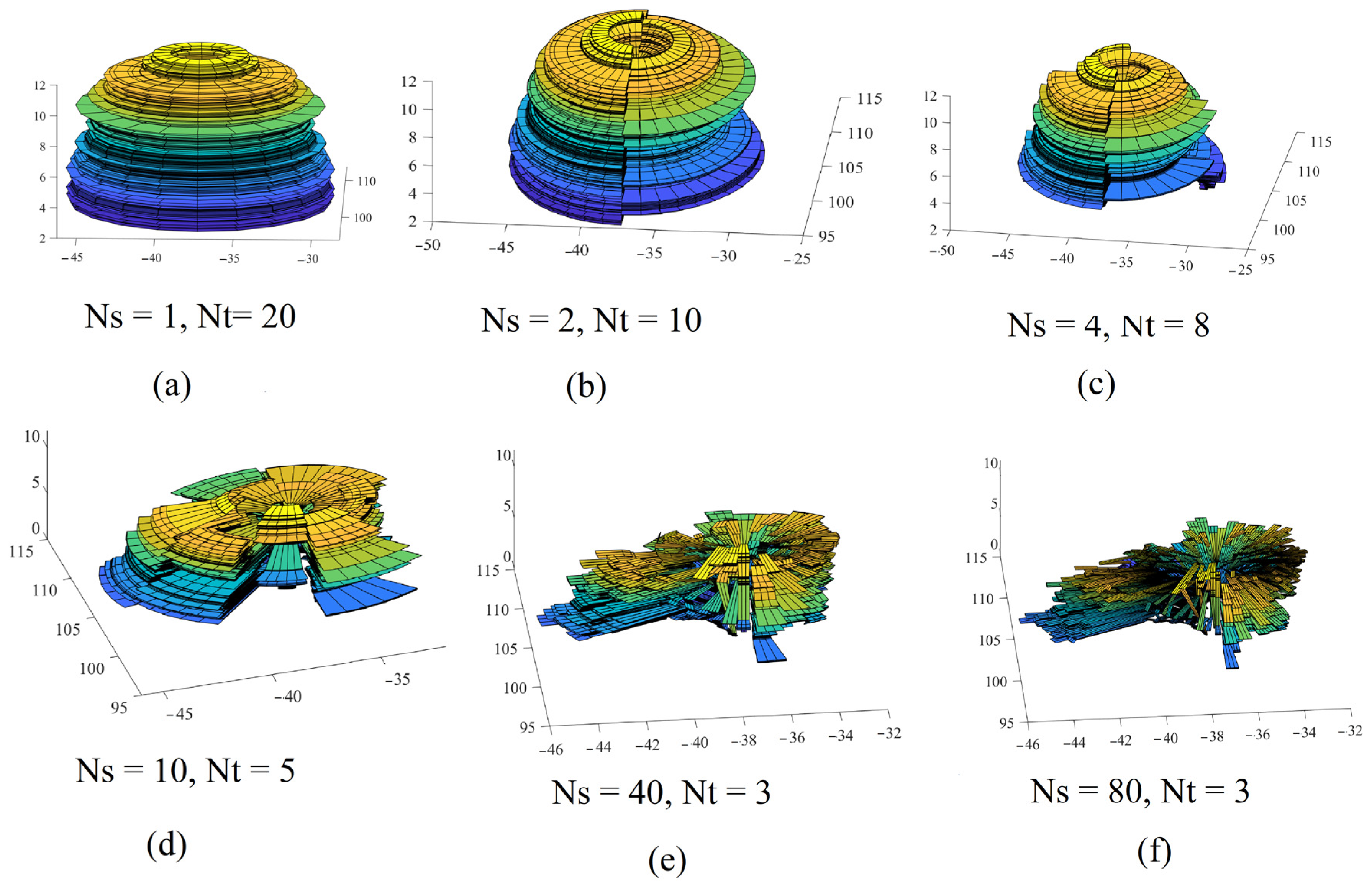
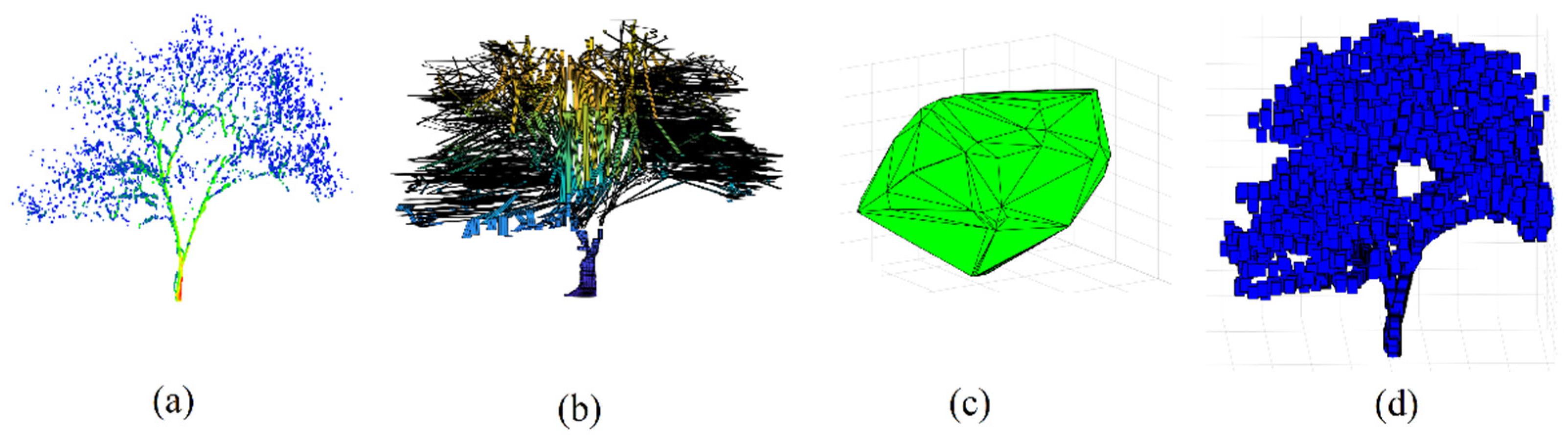
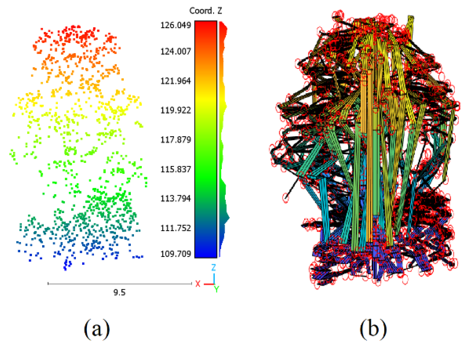
3.2. Crown Biomass Calculation

To calculate the crown biomass starting from the crown point cloud, the approach suggested by Lewandowicz et al. [63], which is based on using the rotating surface principle, will be extended. In the last two cited references, one vertical cross-section from the building point cloud is calculated. Thereafter, the obtained cross-section is rotated around the rotating axis to generate a rotating surface, where the rotating axis is vertical and passes through the crown footprint. The same technique is applied by Lewandowicz et al. [63] to calculate the crown biomass volume. The crown volume in this case will be calculated by the sum of formed frustum of a cone’s volumes. In this context, this approach was not sufficiently accurate because it supposed that the tree crown shape is regular and symmetrical, and it was represented by a rotating surface generated by one of the tree’s vertical cross-sections. In fact, the crown point cloud is not distributed regularly on the tree branches, and the point density is heterogeneous due to the presence of hiding areas as well as the random shape and distribution of tree branches. To conclude, the above-described approach may cause unrealistic oversimplification, which was reflected directly in the low accuracy of the calculated crown volume.

In this paper, the biomass volume calculation approach is improved by minimizing the simplification level through using multi-vertical cross-sections instead of only one cross-section. At this point, it is important to start by calculating the tree crown footprint (Figure 8b). The basic hypothesis is that the Z axis of the coordinate system is vertical or the XY plane is horizontal. If the tree point cloud is already georeferenced, this hypothesis is valid. Otherwise, rotations may be applied on the tree point cloud to guarantee the verticality of the Z axis, which can be completed by a preprocessing step. Hence, the middle of the bounding envelope of the projected point cloud on the plane (OXY) (the tree crown footprint) is pointed using the extreme points coordinates, where this point is named as the footprint gravity center. Thereafter, the maximum distance between the gravity center point and the footprint points is assigned as the footprint radius [62].

Second, once the tree crown footprint is calculated, the crown footprint is divided into identical Ns sectors. This operation allows to divide the crown point cloud into Ns separated point clouds, each of which corresponds to a given sector. In Figure 8c, the tree footprint is divided into four sectors, where Ns = 4. To realize this division, the angle between the line passing through the given point and the gravity center is calculated using Equation (2).

$${\theta }_i=arctan\left(abs(\frac{Y_i-Y_g}{X_i-X_g})\right)+k\frac{\pi }{2}$$

(2)

where $X_i \mathrm{and} Y_i$ are the point coordinates, $X_g \mathrm{and} Y_g$ are the of coordinates of the gravity center, $k$ is a variable that adapts the ${\theta }_i$ value according to its location in the circle quads. In the first quad ${\theta }_i={-\theta }_i+\frac{\pi }{2}$, whereas in the second, third, and fourth quad, $k$ = 3, 2, and 1, respectively.

At this stage, each point is described by its three coordinates $X_i,Y_i \mathrm{and} Z_i$ in addition to the angle ${\theta }_i$. To divide the crown point cloud according to the supposed number of sectors, the point cloud is ascending-sorted according to the $\theta$ angle values. Then, the minimum and maximum $\theta$ angle values for each sector can be assigned. Third, for each crown point, the distance ${\rho }_i$ between the point and the gravity center is calculated according to Equation (3).

$${\rho }_i=\sqrt{{(X_i-X_g)}^2+{(Y_i-Y_g)}^2}$$

(3)

Fourth, the rotating surface is calculated for each sector point cloud independently. Each sector has a minimum ${\theta }_{min}$ angle (beginning angle) and a maximum ${\theta }_{max}$ angle (end angle). Between these two angles, additional Nt internal division angles should be added (Figure 8d). The internal division plays a major role in enhancing the rotating surface when the used number of sectors is small, e.g., Ns = 1, 2, or 20 sectors. In this case, the internal division Nt may be supposed equal to 30, 20, or 10. Conversely, the role of internal division Nt decreases when the used number of sectors is greater, e.g., Ns = 50, 100, or 150 sectors, where the internal division Nt can be supposed equal to 1, 2, or 3. In the next section, the applied number of sectors as well as the number of internal divisions will be discussed in detail because they directly affect the accuracy of biomass calculation.

Fifth, once the number of sectors Ns and the number of internal divisions Nt are assigned, and the crown point cloud is divided according to the supposed number of sectors, the rotating surface of each sector is calculated using the matrixial form (Equations (4)–(6)).

In fact, one rotating surface can be divided into n horizontal slices according to the consecutive Z coordinate values of the cross-section cloud presented into vertical plane O$\rho Z$. The points of each slice have the same Zi coordinate value, which is why all of the elements of each row in the Z matrix are equal. Each slice represents a circle because it belongs to a rotating surface. This circle can be divided into Nt angular sectors. One rotating surface is expressed by three matrices X, Y, and Z. This surface is composed of cells. The coordinates of the middle point of each cell will be considered from the three corresponding cells of the last three matrices. The dimensions of one cell can be calculated as a function of the thickness of the horizontal slice, the Nt value, and the cell circle radius value $\rho$. The application of basic sine and cosine relationships allows deducing the X and Y matrices equations.

$$X_{i,j}=X_g+{\rho }_i\sin {\theta }_j$$

(4)

$$Y_{i,j}=Y_g+{\rho }_i\cos {\theta }_j$$

(5)

$$Z_{i,j}=Z_i$$

(6)

where X, Y, and Z are the rotation surface matrices (I, J), I is the number of vertical cross-section points (n), J is the number of internal divisions Nt, i = 1 to n, j = 1 to Nt.

At this stage, it is important to note that if there are two or more points in the same cross-section having the same Z coordinate value, only the point having greater ${\rho }_i$ is kept, and the other point(s) are removed.

To summarize, one tree point cloud is divided into Ns sector point clouds, and for each sector point cloud, the LiDAR points are presented into the vertical plane O$\rho Z$, which represents a vertical cross-section. These points are descending-sorted according to the Z coordinate values. A rotating surface is calculated from this vertical cross-section using Nt division starting from ${\theta }_{min}$ to ${\theta }_{max}$. This rotating surface is defined by three matrices X, Y, and Z (Equations (4)–(6)). Figure 8e shows the rotating surface of one sector point cloud, whereas Figure 8f shows the complete rotating surfaces of the crown point cloud illustrated in Figure 8a. Figure 9 shows the visualization of the individual sector point clouds model in addition to the complete crown point cloud model, where the model presented in this figure is of the same tree presented in Figure 8.

Finally, the complete tree crown model consists of a list of rotating surfaces, each of which is calculated starting from one division sector point cloud. Since one rotating surface is composed of a list of consecutive frustums of cones, its volume can be calculated by the summation of all frustums of cones forming the crown sector. The crown volume is the summation of rotating surfaces of all sectors (Equation (7)) where BMV is divided by Ns because the calculation is based on the sectors of frustums of the cones.

$$BMV=\frac{\pi }{3\times Ns}\sum _{j=1}^{Ns}\sum _{i=2}^n{h}_{i,j}(R_{i,j}^2+R_{i,j}{R}_{i-1,j}+R_{i-1,j}^2)$$

(7)

where Ns is the number of division sectors, n is the number of rows in matrices presented in Equations (4)–(6), $h_{i,j}$ is the height of frustums of cone sector number i of sector number j; $R_{i,j}$ is the radius of lower base of frustums of the cone sector number i in sector number j; $R_{i-1,j}$ is the radius of upper base of frustums of the cone sector number i of sector number j.

4. Discussion

As mentioned in Section 3.2, the proposed approach of calculating the crown biomass volume suggests dividing the crown point clouds into several sectors and then modeling each sector point cloud independently. When the number of sectors increases, the crown biomass volume becomes more accurate. One question arises at this stage: what is the minimum number of sectors that provides satisfactorily accurate biomass value? To respond to this question, the crown biomass volume is calculated for a variant number of sectors as shown in Figure 10.

From Figure 10 and Figure 11 calculated for the tree crown illustrated in Figure 8, it can be noted that when the number of sectors increases, the crown biomass volume decreases. Indeed, the simplification level for calculating the crown volume decreases and the biomass volume value becomes more accurate and reflects more of the ground truth. Also, when the number of sectors increases, the difference between neighboring crown volume values decreases, and the curve flatness in Figure 10 increases. Moreover, the crown volume difference is almost doubled between the case of Ns =1 sector and Ns = 90 sector.

For Figure 10, it can be noted that when the number of division sectors increases (Figure 11e,f), the tree crown model will look more similar to the tree’s geometric form (Figure 8a). Otherwise, when the number of sectors decreases (Figure 11a–c), the similarity between the tree crown model and the tree geometric form (Figure 8a) will become low.

As the tree crown geometry is discontinuous because it consists of branches and leaves, the biomass calculation algorithm should minimize the inner void volume. When the considered void volume is reduced, the calculation will become more accurate. The suggested approach in the paper reduces such potential estimation errors in the horizontal slices by using a large number of rows in the calculated matrices (Equations (4)–(6)). Similarly, it reduces the void spaces in the vertical cross-sections by using a greater number of division sectors. However, there is a question about the best number of division sectors, which still needs to be determined. Apparently, the number of division sectors may be estimated regarding the tree crown dimensions in addition to the point density. For the same point density, when one tree crown is bigger than another tree crown, the number of division sectors for the bigger tree should be greater than the smaller one. The same concept can be applied to the point density, i.e., for one tree scanned two times with different point densities, the one with a higher point density needs a greater number of division sectors.

In Figure 12, a bounding envelope circle of the crown footprint is shown. The center of this circle is the crown footprint gravity center, and its radius equals the footprint radius (see Section 3.2). The angle $\alpha$ may represent the best sector size when the length of the arc $ab$ equals two times the mean distance separating two neighboring points (mean_dis) (Equations (8) [64] and (9)). This hypothesis is adopted because it is supposed that one sector should contain at least two neighboring points situated on the arc $ab$ when the points are regularly distributed.

$$mea{n}_{dis}=\frac{1}{\sqrt{density}}$$

(8)

$$ab=2\cdot {mean}_{dis}$$

(9)

To calculate the mean_dis, it is unadvised to use the theoretical point density provided by the scanning company because this point cloud may contain a considerable number of duplicated points [65]. For this purpose, the tree crown point cloud should first be filtered, and all duplicated points must be removed. Thereafter, the number of remaining crown points is divided by the bounding envelope of the circler area. In this case, the obtained point density will be more realistic. Thus, the application of Equations (8) and (9) allows for obtaining the distance length $ab$ (Figure 12), supposing that the arc length is similar to the straight length attaching the points “a” and “b” (Equation (10)). From the arc $ab$ length and the circle radius R values, the angle $\alpha$ can be calculated (Equation (11)). Once the angle $\alpha$ is calculated, the number of sectors (Ns) can be deduced (Equation (12)).

$$mea{n}_{dis}=\frac{\sqrt{\pi }R}{\sqrt{n}}$$

(10)

$${\alpha }_{Rad}=\frac{\sqrt{\pi }}{\sqrt{n}}$$

(11)

$$Ns=2\sqrt{n\cdot \pi }$$

(12)

where $n$ is the number of crown points after filtering, $R$ is the radius of the bounding envelope circle of tree crown footprint.

At this stage, it is important to note that the crown point cloud is filtered only to calculate the number of division sectors. For calculating the BioMass Volume (BMV), it can be employed without filtering. However, it can be noted from Equation (12) that the number of division sectors is related only to the number of crown points after removing the duplicate points. As an example, for the tree shown in Figure 8, R = 9.4 m, mean_dis = 0.2 m, the original number of points is 5754, the number of points after filtering is 1926, Ns = 155 sectors. BMV = 211.9 m³. Finally, the flat long tail of the curve shown in Figure 10 happens when the number of points of the crown point cloud is huge, which is the case when static terrestrial laser scanning is used. In this example, the obtained number of sectors is more than 360 sectors, and we then can accept Ns value equal to 300.

Finally, concerning the trunk volume calculation, the considered slices are thin. The trunk is not always distinguishable, and the trunk volume is small in the general cases regarding the crown volume. That is why the slice geometric form is supposed cylindrical. Unfortunately, the trunk modeling method is still suffering from limitations because the extended RANSAC paradigm sometimes does not provide faithful results for detecting circler arcs. The influence of this error is still limited because the trunk volume is small in comparison to the crown volume.

To conclude, the suggested approach contains two kinds of parameters, the trunk modeling parameters, and the crown modeling parameters. Concerning the trunk parameters, they are presented, discussed, and detailed by Tarsha Kurdi et al. [56]. For the crown parameters, there are two main parameters which are the number of sectors (Ns) and the number of internal divisions (Nt). Ns is calculated from Equation (12) whereas the value of Nt is supposed a constant equal to 3.

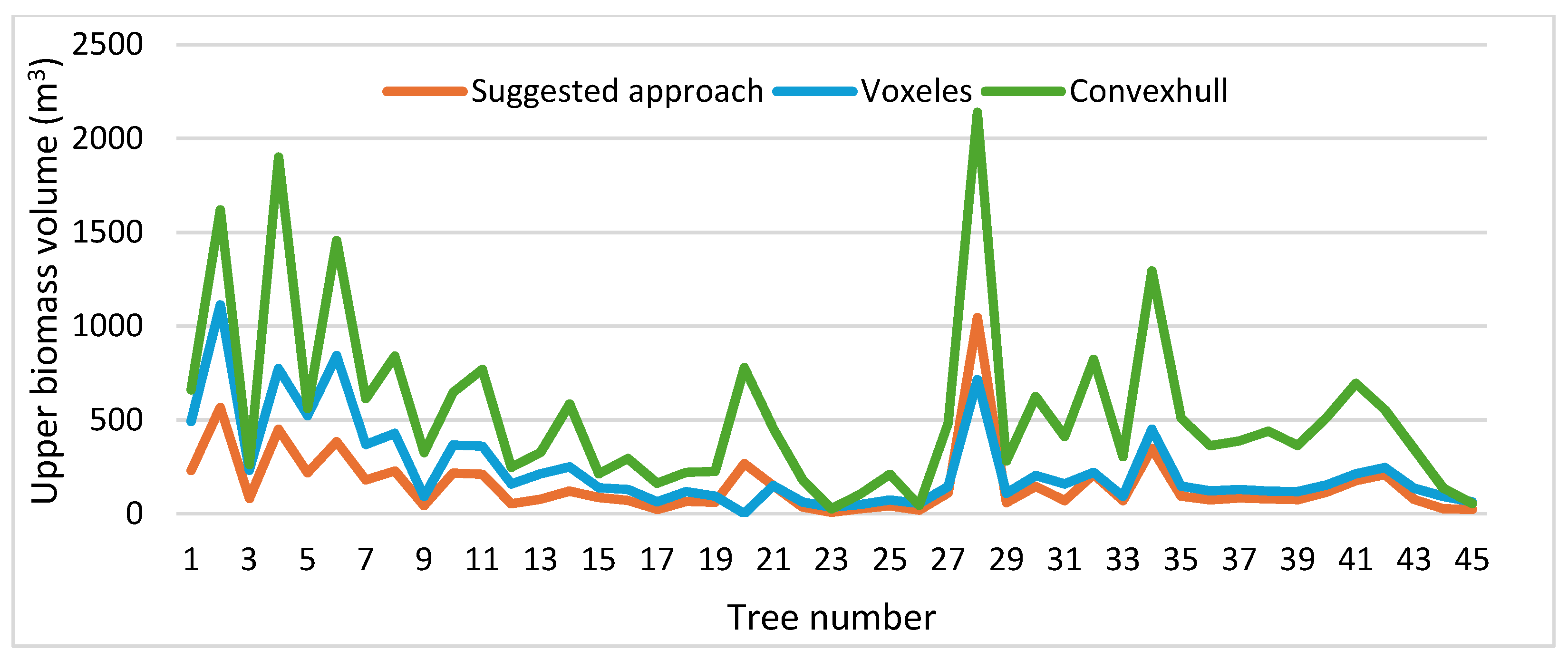
5. Accuracy Analysis

To assess the accuracy of the suggested approach for calculating a tree’s upper biomass volume, the obtained results by the suggested approach are first compared with two other methods, the voxelization of tree point cloud and convex hull. Second, the tree model used to calculate the upper biomass volume will be compared with the constructed tree model with the point cloud as a reference model.

Figure 13 illustrates the difference between the tree models constructed by the proposed algorithm, the voxelization of the tree point cloud, and the convex hull approach. It can be noted that the convex hull model (Figure 13c) dislikes the actual tree geometry, which is why the values of biomass volume shown in Figure 14 are much greater than the other two algorithms. Moreover, despite the similarity of the tree model calculated by the voxelization approach with the actual tree geometry (Figure 13d), this algorithm neglects the hidden areas (voids) in the tree crown and handles the tree crown and trunk in the same way (Figure 13d). Also, the problem of determination of voxel resolution may play a major role in obtaining an overestimation of the biomass volume as shown in Figure 14. The volume overestimation can take minimum values such as Tree number 26 or maximum values such as Tree number 28 in Figure 14. In contrast, the suggested approach constructs a 3D tree model by considering the crucial difference in geometric form between the crown and the trunk. The division of the tree point clouds into sectors not only allows for an accurate simulation of the tree geometry, but also helps to reduce the biomass overestimation by avoiding the void spaces in the tree model (Figure 13b). That is why most of the tested tree samples in Figure 14 provide minimum biomass volume using the suggested approach. To conclude, Figure 10 shows that the proposed algorithm minimizes the tree biomass overestimation regarding the two other compared approaches.

To assess the accuracy of the estimated biomass, we visualize the superimposition of tree point clouds on the constructed tree model developed in this paper (Figure 15), where the former is used as a reference [66,67]. It can be noted that the constructed 3D tree crown model fits the point cloud accurately because this model is calculated to pass through all crown points. Otherwise, the trunk model may have deviations from the trunk point cloud of about 5.6 cm [56]. Indeed, these deviations are due to fitting the cylinders composed of the trunk body. Nevertheless, the fact that using two different modeling approaches to model the crown and the trunk plays an important role in increasing the calculation accuracy of the upper biomass volume.

Finally, it is unavoidable that the accuracy of the biomass volume calculation is related to the accuracy of the suggested tree model. Hence, one tree model consists of matrices of cells linked through robust neighbor relationships. To examine the accuracy of a tree model, the approach suggested by Tarsha Kurdi et al. [55] is applied. This method uses the mean cell dimensions as an evaluation metric. The cell dimensions are the Cell Width (C_W) and the Cell Height (C_H). Moreover, the Relative Absolute Errors (RAE) of C_H and C_W are calculated, where the mean C_H is divided by the tree height (H_t) and the mean C_W is divided by the tree footprint perimeter (Per). In this context, the first five trees in Figure 10 are selected.

To carry out this calculation, it is supposed that all sectors’ matrices are merged into one matrix. The number of columns of this matrix is related to the number of division sectors. Furthermore, the C_W value is related to the number of columns in addition to the distance from the tree footprint gravity center. Apparently, when the number of columns of the crown model matrices increases, the cell width will decrease. Furthermore, C_W and C_H values may change from one point to another in the tree model. Indeed, for each tree model, the minimum, maximum, and mean values of C_W and C_H are estimated (

Table 1. Accuracy of the tree models using matrix cell dimensions.

	Tree Width Error				Tree Height Error
Tree No.	Min (m)	Max (m)	Mean (m)	$\frac{{\mathit{C}}_{\mathit{W}}\times 100}{\mathit{P}\mathit{e}\mathit{r}}$	Min (m)	Max (m)	Mean (m)	$\frac{{\mathit{C}}_{\mathit{H}}\times 100}{{\mathit{H}}_{\mathit{t}}}$
1	0.01	0.29	0.15	0.28	0.01	0.02	0.01	0.01
2	0.01	0.49	0.22	0.27	0.01	0.27	0.02	0.00
3	0.01	0.23	0.11	0.27	0.01	0.04	0.01	0.01
4	0.01	0.42	0.15	0.23	0.01	0.01	0.01	0.00
5	0.01	0.14	0.07	0.29	0.01	0.08	0.01	0.00

Per: is the footprint perimeter; H_t is the tree height.

). However, C_W and C_H can reflect the accuracy of the cell position within the calculated tree model. One LiDAR point is hypothetical to be placed in the cell center, but in practice, it may be situated everywhere inside the cell. Finally, the values of Table 1 confirm the high accuracy of calculated tree models, and as a consequence, the high accuracy of the calculated crown biomass.

6. Conclusions

The suggested approach in this paper modeled the trunk and the crown using two distinguished approaches regarding their different geometric nature. The results of comparison to the previously reported methods in the literature, as well as the high accuracy of the suggested approach, where the maximum absolute quantitative error equals 0.49 m, and the maximum relative absolute error equals 0.29%, confirmed the efficacity of the proposed biomass volume estimation method. Unfortunately, some limitations are still present, such as the sensitivity of the trunk modeling method, where the extended RANSAC paradigm sometimes does not provide faithful results for detecting circler arcs. Moreover, the heterogenetic distribution of LiDAR points may produce errors in biomass volume estimation. All these limitations present research questions for future work. Furthermore, it is still necessary to develop an algorithm for automatic tree detection and filtering starting from the vegetation mask of the LiDAR point cloud. This procedure will allow the completion of the fully automatic operation for forest monitoring. Finally, it is necessary to further test the proposed algorithm with wide datasets, such as Unmanned Arial Vehicle (UAV) LiDAR data and Simultaneous Localization And Mapping (SLAM) data.

References

1. Tao, F.; Xiao, B.; Qi, Q.; Cheng, J.; Ji, P. Digital twin modeling. J. Manuf. Syst. 2022, 64, 372–389. [Google Scholar] [CrossRef]
2. Hakimi, O.; Liu, H.; Abudayyeh, O.; Houshyar, A.; Almatared, M.; Alhawiti, A. Data Fusion for Smart Civil Infrastructure Management: A Conceptual Digital Twin Framework. Buildings 2023, 13, 2725. [Google Scholar] [CrossRef]
3. Ahmad, A.M.; Aliyu, A.A. The need for landscape information modelling (LIM) in landscape architecture. In Proceedings of the 13th Digital Landscape Architecture Conference, Weimar, Germany, 31 May–2 June 2012; p. 40. [Google Scholar]
4. Song, J.; Park, S.; Lee, K.; Bae, J.; Kwon, S.; Cho, C.-S.; Chung, S. Augmented Reality-Based BIM Data Compatibility Verification Method for FAB Digital Twin implementation. Buildings 2023, 13, 2683. [Google Scholar] [CrossRef]
5. Mylo, M.D.; Ludwig, F.; Rahman, M.A.; Shu, Q.; Fleckenstein, C.; Speck, T.; Speck, O. Conjoining. Trees for the Provision of Living Architecture in Future Cities: A Long-Term Inosculation Study. Plants 2023, 12, 1385. [Google Scholar] [CrossRef]
6. Song, Q.; Albrecht, C.M.; Xiong, Z.; Zhu, X.X. Towards Global Forest Biomass Estimators from Tree Height Data. In Proceedings of the IGARSS 2022–2022 IEEE International Geoscience and Remote Sensing Symposium, Kuala Lumpur, Malaysia, 17–22 July 2022; pp. 5652–5655. [Google Scholar] [CrossRef]
7. Antropov, O.; Rauste, Y.; Tegel, K.; Baral, Y.; Junttila, V.; Kauranne, T.; Hame, T.; Praks, J. Tropical Forest Tree Height and Above Ground Biomass Mapping in Nepal Using Tandem-X and ALOS PALSAR Data. In Proceedings of the IGARSS 2018–2018, IEEE International Geoscience and Remote Sensing Symposium, Valencia, Spain, 22–27 July 2018; pp. 5334–5336. [Google Scholar] [CrossRef]
8. Acuna, M.; Sessions, J.; Zamora, R.; Boston, K.; Brown, M.; Ghaffariyan, M.R. Methods to Manage and Optimize Forest Biomass Supply Chains: A Review. Curr. For. Rep. 2019, 5, 124–141. [Google Scholar] [CrossRef]
9. Xu, D.; Wang, H.; Xu, W.; Luan, Z.; Xu, X. LiDAR Applications to Estimate Forest Biomass at Individual Tree Scale: Opportunities, Challenges and Future Perspectives. Forests 2021, 12, 550. [Google Scholar] [CrossRef]
10. Solano-Correa, Y.T.; Camacho-De Angulo, Y.V.; Oviedo-Barrero, F.; Dalponte, M.; Pencue-Fierro, E.L. Individual Tree Crown Delineation and Biomass Estimation from LiDAR Data in Gorgona Island, Colombia. In Proceedings of the IGARSS 2023–2023 IEEE International Geoscience and Remote Sensing Symposium, Pasadena, CA, USA, 16–21 July 2023; pp. 3125–3128. [Google Scholar] [CrossRef]
11. Uciechowska-Grakowicz, A.; Herrera-Granados, O.; Biernat, S.; Bac-Bronowicz, J. Usage of Airborne LiDAR Data and High-Resolution Remote Sensing Images in Implementing the Smart City Concept. Remote Sens. 2023, 15, 5776. [Google Scholar] [CrossRef]
12. Ketterings, Q.M.; Coe, R.; van Noordwijk, M.; Ambagau’, Y.; A Palm, C. Reducing uncertainty in the use of allometric biomass equations for predicting above-ground tree biomass in mixed secondary forests. For. Ecol. Manag. 2001, 146, 199–209. [Google Scholar] [CrossRef]
13. Beer, C.; Reichstein, M.; Tomelleri, E.; Ciais, P.; Jung, M.; Carvalhais, N.; Rödenbeck, C.; Arain, M.A.; Baldocchi, D.; Bonan, G.B.; et al. Terrestrial gross carbon dioxide uptake: Global distribution and covari-ation with climate. Science 2010, 329, 834–839. [Google Scholar] [CrossRef]
14. Bac-Bronowicz, J.; Uciechowska-Grakowicz, A.; Biernat, S.; Bidzińska, P.; Górecki, A.; Przybyła, T.; Rosicki, M.; Załupka, M. System Ewaluacji Usług Ekosystemowych Zieleni Miejskiej (System for Evaluating Ecosystem Services of Urban Greenery); Oficyna Wydawnicza Politechniki Wrocławskiej: Wrocław, Poland, 2022; pp. 108–110. ISBN 978-83-7493-214-1. Available online: https://www.oficyna.pwr.edu.pl (accessed on 26 March 2024).
15. Price, J. Estimating leaf area index from satellite data. IEEE Trans. Geosci. Remote. Sens. 1993, 31, 727–734. [Google Scholar] [CrossRef]
16. Bochenek, Z.; Dąbrowska-Zielińska, K.; Gurdak, R.; Niro, F.; Bartold, M.; Grzybowski, P. Validation of the LAI biophysical product derived from Sentinel-2 and Proba-V images for winter wheat in western Poland. Geoinformation 2017, 1, 15–26. [Google Scholar] [CrossRef]
17. Fang, H.; Baret, F.; Plummer, S.; Schaepman-Strub, G. An overview of global leaf area index (LAI): Methods, products, validation, and applications. Rev. Geophys. 2019, 57, 739–799. [Google Scholar] [CrossRef]
18. De Bock, A.; Belmans, B.; Vanlanduit, S.; Blom, J.; Alvarado-Alvarado, A.A.; Audenaert, A. A review on the leaf area index (LAI) in vertical greening systems. Build. Environ. 2023, 229, 109926. [Google Scholar] [CrossRef]
19. Weiss, M.; Baret, F.; Smith, G.J.; Jonckheere, I.; Coppin, P. Review of methods for in situ leaf area index (LAI) determination: Part II. Estimation of LAI, errors and sampling. Agric. For. Meteorol. 2003, 121, 37–53. [Google Scholar] [CrossRef]
20. Zani, N.F.; Suratman, M.N. Estimation of above ground biomass of Keniam forests, Taman Negara Pahang. In Proceedings of the IEEE Symposium on Business, Engineering and Industrial Applications (ISBEIA), Langkawi, Malaysia, 25–28 September 2011; pp. 80–83. [Google Scholar] [CrossRef]
21. Kato, R.; Tadaki, Y.; Ogawa, H. Plant biomass and growth increment studies in Pasoh Forest Reserve. Malay. Nat. J. 1978, 30, 211–224. Available online: https://api.semanticscholar.org/CorpusID:82565727 (accessed on 26 March 2024).
22. Lei, X.; Zhang, H.; Bi, H. Additive aboveground biomass equations for major tree species in over-logged forest region in northeast China. In Proceedings of the IEEE 4th International Symposium on Plant Growth Modeling, Simulation, Visualization and Applications, Shanghai, China, 31 October–3 November 2012; pp. 220–223. [Google Scholar] [CrossRef]
23. Tchinmegni, F.I.; Djeukam, P.S.V. Allometric models for estimating above- and belowground biomass of individual trees in Cameroonian submontane forest. MOJ Eco Environ. Sci. 2024, 9, 29–36. [Google Scholar] [CrossRef]
24. Gaikadi, S.; Selvaraj, V.K. Allometric model based estimation of biomass and carbon stock for individual and overlapping trees using terrestrial LiDAR. Model. Earth Syst. Environ. 2024, 10, 1771–1782. [Google Scholar] [CrossRef]
25. Cao, L.; Coops, N.C.; Sun, Y.; Ruan, H.; Wang, G.; Dai, J.; She, G. Estimating canopy structure and biomass in bamboo forests using airborne LiDAR data. ISPRS J. Photogramm. Remote Sens. 2019, 148, 114–129. [Google Scholar] [CrossRef]
26. Zhang, Q.; Xu, L.; Zhang, M.; Wang, Z.; Gu, Z.; Wu, Y.; Shi, Y.; Lu, Z. Uncertainty Analysis of Remote Sensing Pretreatment for Biomass Estimation on Landsat OLI and Landsat ETM+. ISPRS Int. J. Geo-Inf. 2020, 9, 48. [Google Scholar] [CrossRef]
27. Kumar, P.; Krishna, A.P.; Rasmussen, T.M.; Pal, M.K. Rapid Evaluation and Validation Method of Above Ground Forest Biomass Estimation Using Optical Remote Sensing in Tundi Reserved Forest Area, India. ISPRS Int. J. Geo-Inf. 2021, 10, 29. [Google Scholar] [CrossRef]
28. Stratoulias, D.; Nuthammachot, N.; Suepa, T.; Phoungthong, K. Assessing the Spectral Information of Sentinel-1 and Sentinel-2 Satellites for Above-Ground Biomass Retrieval of a Tropical Forest. ISPRS Int. J. Geo-Inf. 2022, 11, 199. [Google Scholar] [CrossRef]
29. Dong, L.; Du, H.; Han, N.; Li, X.; Zhu, D.; Mao, F.; Zhang, M.; Zheng, J.; Liu, H.; Huang, Z.; et al. Application of Convolutional Neural Network on Lei Bamboo Above-Ground-Biomass (AGB) Estimation Using Worldview-2. Remote Sens. 2020, 12, 958. [Google Scholar] [CrossRef]
30. Zhao, H.; Morgenroth, J.; Pearse, G.; Schindler, J. A Systematic Review of Individual Tree Crown Detection and Delineation with Convolutional Neural Networks (CNN). Curr. For. Rep. 2023, 9, 149–170. [Google Scholar] [CrossRef]
31. Michałowska, M.; Rapiński, J. A Review of Tree Species Classification Based on Airborne LiDAR Data and Applied Classifiers. Remote Sens. 2021, 13, 353. [Google Scholar] [CrossRef]
32. Weinmann, M.; Weinmann, M.; Mallet, C.; Brédif, M. A Classification-Segmentation Framework for the Detection of Individual Trees in Dense MMS Point Cloud Data Acquired in Urban Areas. Remote. Sens. 2017, 9, 277. [Google Scholar] [CrossRef]
33. Lindberg, E.; Holmgren, J. Individual Tree Crown Methods for 3D Data from Remote Sensing. Curr. For. Rep. 2017, 3, 19–31. [Google Scholar] [CrossRef]
34. Meschin, K. Canopy Gap Fraction Estimation from ICESat-2 ATL08 Product. Master’s Thesis, Delft University of Technology, Delft, The Netherlands, 2023. Available online: https://resolver.tudelft.nl/uuid:4c44f0fb-bd69-44d8-8ba9-6ae0b9584828 (accessed on 26 March 2024).
35. Chen, Z.; Xu, B.; Devereux, B. Urban landscape pattern analysis based on 3D landscape models. Appl. Geogr. 2014, 55, 82–91. [Google Scholar] [CrossRef]
36. Raich, J.W.; Nadelhoffer, K.J. Belowground Carbon Allocation in Forest Ecosystems: Global Trends. Ecology 1989, 70, 1346–1354. [Google Scholar] [CrossRef]
37. Cui, X.; Guo, L.; Chen, J.; Chen, X.; Zhu, X. Estimating Tree-Root Biomass in Different Depths Using Ground-Penetrating Radar: Evidence from a Controlled Experiment. IEEE Trans. Geosci. Remote. Sens. 2013, 51, 3410–3423. [Google Scholar]
38. Zhou, L.; Li, X.; Zhang, B.; Xuan, J.; Gong, Y.; Tan, C.; Huang, H.; Du, H. Estimating 3D Green Volume and Aboveground Biomass of Urban Forest Trees by UAV-Lidar. Remote Sens. 2022, 14, 5211. [Google Scholar] [CrossRef]
39. Lin, Y.; Jaakkola, A.; Hyyppä, J.; Kaartinen, H. From TLS to VLS: Biomass Estimation at Individual Tree Level. Remote Sens. 2010, 2, 1864–1879. [Google Scholar] [CrossRef]
40. Kato, A.; Moskal, L.M.; Schiess, P.; Swanson, M.E.; Calhoun, D.; Stuetzle, W. Capturing tree crown formation through implicit surface reconstruction using airborne lidar data. Remote Sens. Environ. 2016, 113, 1148–1162. [Google Scholar] [CrossRef]
41. Reckziegel, R.B.; Larysch, E.; Sheppard, J.P.; Kahle, H.P.; Morhart, C. Modelling and Comparing Shading Effects of 3D Tree Structures with Virtual Leaves. Remote. Sens. 2021, 13, 532. [Google Scholar] [CrossRef]
42. Yan, Z.; Liu, R.; Cheng, L.; Zhou, X.; Ruan, X.; Xiao, Y. A Concave Hull Methodology for Calculating the Crown Volume of Individual Trees Based on Vehicle-Borne LiDAR Data. Remote. Sens. 2019, 11, 623. [Google Scholar] [CrossRef]
43. Hackenberg, J.; Spiecker, H.; Calders, K.; Disney, M.; Raumonen, P. SimpleTree—An Efficient Open-Source Tool to Build Tree Models from TLS Clouds. Forests 2015, 6, 4245–4294. [Google Scholar] [CrossRef]
44. CityGML–Open Geospatial Consortium. (n.d.). Retrieved 19 April 2023. Available online: https://www.ogc.org/standard/citygml/ (accessed on 26 March 2024).
45. Ortega-Córdova, L. Urban Vegetation Modeling 3D Levels of Detail. 2018 Degree Granting Institution. Master’s Thesis, Delft University of Technology, Delft, The Netherlands, 2018. Available online: https://repository.tudelft.nl/islandora/object/uuid:8b8967a8-0a0f-498f-9d37-71c6c3e532af?collection=education (accessed on 26 March 2024).
46. Wei, Z.; Li, X.; He, Z. Semantic Urban Vegetation Modelling Based on an Extended CityGML Description. In Proceedings of the 2022 Digital Landscape Architecture Conference, Boston, MA, USA, 9 June 2022; pp. 200–212. [Google Scholar] [CrossRef]
47. Zhu, C.; Zhang, X.; Hu, B.; Jaeger, M. Reconstruction of tree crown shape from scanned data. In Lecture Notes in Computer Science (Including Subseries Lecture Notes in Artificial Intelligence and Lecture Notes in Bioinformatics); Springer: Berlin/Heidelberg, Germany, 2008; Volume 5093, pp. 745–756. [Google Scholar] [CrossRef]
48. Zhen, Z.; Quackenbush, L.J.; Zhang, L.; Swatantran, A.; Baghdadi, N.; Thenkabail, P.S. Trends in Automatic Individual Tree Crown Detection and Delineation—Evolution of lidar Data. Remote Sens. 2016, 8, 333. [Google Scholar] [CrossRef]
49. Dai, M.; Li, G. Soft Segmentation and Reconstruction of Tree Crown from Laser Scanning Data. Electronics 2023, 12, 2300. [Google Scholar] [CrossRef]
50. Du, S.; Lindenbergh, R.; Ledoux, H.; Stoter, J.; Nan, L. AdTree: Accurate, Detailed, and Automatic Modelling of Laser-Scanned Trees. Remote Sens. 2019, 11, 2074. [Google Scholar] [CrossRef]
51. Huang, Z.; Huang, X.; Fan, J.; Eichhorn, M.P.; An, F.; Chen, B.; Cao, L.; Zhu, Z.; Yun, T. Retrieval of Aerodynamic Parameters in Rubber Tree Forests Based on the Computer Simulation Technique and Terrestrial Laser Scanning Data. Remote Sens. 2020, 12, 1318. [Google Scholar] [CrossRef]
52. Liang, X.; Kankare, V.; Hyyppa, J.; Wang, Y.; Kuuo, A.; Vastaranta, M. Terresial laser scanning in forest inventories. ISPRS J. Photogramm. Remote. Sens. 2016, 115, 63–77. [Google Scholar] [CrossRef]
53. Angel, E. Interactive Computer Graphics a Top-Down Approach with OpenGL; Addison Wesley: Boston, MA, USA, 2003; pp. 559–593, ISBN-13 978-0-13-254523-5. [Google Scholar]
54. Syed Ahmad, S.S.; Mohd Mushar, S.H.; Zamah Shari, N.H.; Kasmin, F. A Comparative study of log volume estimation by using statistical method. Educ. J. Sci. Math. Technol. 2020, 7, 22–28. [Google Scholar] [CrossRef]
55. Tarsha Kurdi, F.; Lewandowicz, E.; Shan, J.; Gharineiat, Z. Three-dimensional modeling and visualization of single tree LiDAR point cloud using matrixial form. IEEE J. Sel. Top. Appl. Earth Obs. Remote. Sens. 2024, 17, 3010–3022. [Google Scholar] [CrossRef]
56. Kurdi, F.T.; Gharineiat, Z.; Lewandowicz, E.; Shan, J. Modeling the Geometry of Tree Trunks Using LiDAR Data. Forests 2024, 15, 368. [Google Scholar] [CrossRef]
57. Fernández-Sarría, A.; Martínez, L.; Velázquez-Martí, B.; Sajdak, M.; Estornell, J.; Recio, J.A. Different methodologies for calculating crown volumes of Platanus hispanica trees using terrestrial laser scanner and a comparison with classical dendrometric measurements. Comput. Electron. Agric. 2013, 90, 176–185. [Google Scholar] [CrossRef]
58. Food and Agriculture Organisation. Available online: www.fao.org (accessed on 11 March 2024).
59. Lewandowicz, E.; Antolak, M. Converting database on dendrological objects of Kortowo campus at the University of Warmia and Mazury in Olsztyn to current GIS standards. In Proceedings of the 15th International Multidisciplinary Scientific GeoConference SGEM 2015, Albana, Bulgaria, 18–24 June 2015; Volume 2, pp. 787–794. [Google Scholar]
60. Salekin, S.; Catalán, C.H.; Boczniewicz, D.; Phiri, D.; Morgenroth, J.; Meason, D.F.; Mason, E.G. Global Tree Taper Modelling: A Review of Applications, Methods, Functions, and Their Parameters. Forests 2021, 12, 913. [Google Scholar] [CrossRef]
61. Larsen, D.R. Simple taper: Taper equations for the field forester. In Proceedings of the 20th Central Hardwood Forest Conference, Newtown Square, PA, USA, 28 March–1 April 2016; Kabrick, J.M., Dey, D.C., Knapp, B.O., Larsen, D.R., Shifley, S.R., Stelzer, H.E., Eds.; Columbia, MO. General Technical Report NRS-P-167. U.S. Department of Agriculture, Forest Service, Northern Research Station: Newtown Square, PA, USA, 2016; pp. 265–278. [Google Scholar]
62. Tarsha Kurdi, F.; Landes, T.; Grussenmeyer, P. Extended RANSAC algorithm for automatic detection of building roof planes from Lidar data. Photogramm. J. Finl. 2008, 21, 97–109. [Google Scholar]
63. Lewandowicz, E.; Tarsha Kurdi, F.; Gharineiat, Z. 3D LoD2 and LoD3 modeling of buildings with ornamental towers and turrets based on LiDAR data. Remote Sens. 2022, 14, 4687. [Google Scholar] [CrossRef]
64. Tarsha Kurdi, F.; Landes, T.; Grussenmeyer, P.; Smigiel, E. New approach for automatic detection of buildings in airborne laser scanner data using first echo only. Eng. Environ. Sci. 2006, 36, 25–30. [Google Scholar]
65. Tarsha Kurdi, F.; Reed, P.; Gharineiat, Z.; Awrangjeb, M. Efficiency of terrestrial laser scanning in survey works: Assessment, modelling, and monitoring. Int. J. Environ. Sci. Nat. Resour. 2023, 32, 556334. [Google Scholar] [CrossRef]
66. Tarsha Kurdi, F.; Awrangjeb, M. Comparison of LiDAR building point cloud with reference model for deep comprehension of cloud structure. Can. J. Remote Sens. 2020, 46, 603–621. [Google Scholar] [CrossRef]
67. Ostrowski, W.; Pilarska, M.; Charyton, J.; Bakuła, K. Analysis of 3D building models accuracy based on the airborne Laser scanning point clouds. Int. Arch. Photogramm. Remote Sens. Spat. Inf. Sci. 2018, 42, 797–804. [Google Scholar] [CrossRef]
Figure 1. Examples of solid models for tree crown modeling: (a) geometric solids, (b) tree crown models [45].
Remotesensing 16 02220 g001
Figure 2. Visualization of the wrapped surface reconstruction. Shown are tulip-tree and atlas cedar [53].
Remotesensing 16 02220 g002
Figure 3. Algorithms for modeling tree crown hulls [33].
Remotesensing 16 02220 g003
Figure 4. The single crown tree contour constructed by the concave hull with different parameters [38].
Remotesensing 16 02220 g004
Figure 5. Visualization of a tree crown formation captured by the artwork of Christo and Jean-Claude. (Christo and Jeanne-Claude, Wrapped Trees, Fondation Beyeler and Berower Park, Riehen, Switzerland 1997–1998, Photo: Wolfgang Volz, ©Christo 1998) [40].
Remotesensing 16 02220 g005
Figure 6. Flowchart of the suggested algorithm for upper biomass calculation; gray boxes were developed by Tarsha Kurdi et al. [56]. R 2 is the radius of lower base of frustums of the cone; R 1 is the radius of upper base of frustums of the cone; h is the height of the cylinder and frustums of the cone; r is the radius of the cylinder base.
Remotesensing 16 02220 g006
Figure 7. Trunk modeling; (a) tree point cloud; (b) segmentation of tree point cloud into trunk and crown point clouds; (c) 3D trunk model.
Remotesensing 16 02220 g007
Figure 8. Division of tree footprint into sectors; (a) tree point cloud; (b) tree footprint; (c) division of tree footprint into four sectors; (d) division of one sector into three internal sections; (e) 3D model of one sector in (c); (f) 3D model of four sectors in (c); Ns is the number of division sectors; Nt is the number of internal divisions.
Remotesensing 16 02220 g008
Figure 9. Visualization of a sector point cloud model. The tree crown is divided into four sectors with (ad) for individual sector models, and (e) for the complete crown model.
Remotesensing 16 02220 g009
Figure 10. Crown biomass volume (m3) for different number of sectors. This curve is calculated for the tree presented in Figure 8.
Remotesensing 16 02220 g010
Figure 11. Three-dimensional models of a tree crown using different numbers of vertical cross-sections (Ns); (a) Ns = 1; (b) Ns = 2; (c) Ns = 4; (d) Ns = 10; (e) Ns = 40; (f) Ns = 80; These models are calculated for the same tree point cloud shown in Figure 8.
Remotesensing 16 02220 g011
Figure 12. Calculation of best sector angle (α); A bounding envelope circle of a tree crown footprint; R is bounding envelope circle radius.
Remotesensing 16 02220 g012
Figure 13. Tree models for calculating upper biomass; (a) tree point cloud; (b) tree model from this study; (c) convex hull tree model; (d) voxel tree model.
Remotesensing 16 02220 g013
Figure 14. Comparison of upper biomass volume calculated by three approaches: this study, voxelization, and convex hull.
Remotesensing 16 02220 g014
Figure 15. Superimpose of tree point cloud on the derived tree model. (a) Tree point cloud; (b) Point cloud laying on tree model for biomass calculation. The colours in (a) are calculated as a function of the Z coordinate values, where the red circles in (b) represent the LiDAR points.
Remotesensing 16 02220 g015