Decomposition of Submesoscale Ocean Wave and Current Derived from UAV-Based Observation

Abstract

The consecutive submesoscale sea surface processes observed by an unmanned aerial vehicle (UAV) were used to decompose into spatial waves and current features. For the image decomposition, the Fast and Adaptive Multidimensional Empirical Mode Decomposition (FA-MEMD) method was employed to disintegrate multicomponent signals identified in sea surface optical images into modulated signals characterized by their amplitudes and frequencies. These signals, referred to as Bidimensional Intrinsic Mode Functions (BIMFs), represent the inherent two-dimensional oscillatory patterns within sea surface optical data. The BIMFs, separated into seven modes and a residual component, were subsequently reconstructed based on the physical frequencies. A two-dimensional Fast Fourier Transform (2D FFT) for each high-frequency mode was used for surface wave analysis to illustrate the wave characteristics. Wavenumbers (K_x, K_y) ranging between 0.01–0.1 radm⁻¹ and wave directions predominantly in the northeastward direction were identified from the spectral peak ranges. The Optical Flow (OF) algorithm was applied to the remaining consecutive low-frequency modes as the current signal under 0.1 Hz for surface current analysis and to estimate a current field with a 1 m spatial resolution. The accuracy of currents in the overall region was validated with in situ drifter measurements, showing an R-squared (R²) value of 0.80 and an average root-mean-square error (RMSE) of 0.03 ms⁻¹. This study proposes a novel framework for analyzing individual sea surface dynamical processes acquired from high-resolution UAV imagery using a multidimensional signal decomposition method specialized in nonlinear and nonstationary data analysis.

1. Introduction

Submesoscale ocean processes with spatial scales of 0.1–10 km serve as a key intermediary between larger-scale balanced dynamics and unbalanced turbulence [1,2]. These scales contribute significantly to ocean kinetic energy via circulation [3,4], playing a particularly essential role in energy transfer from mesoscale to small-scale turbulence [5,6] and providing a route for dissipation [7] and mixing [6,8], vertical density stratification or re-stratification [9,10], and facilitating biological processes in the ocean [11,12], which demonstrates its function as a fundamental driver of ocean dynamic phenomena. Therefore, it is essential to understand the role of each submesoscale dynamic in bridging the gap between diverse motion and connection scales among multiscale interactions [1,2,11,12,13]. However, relatively short-term submesoscale phenomena that last from hours to days require a high spatiotemporal resolution to determine their detailed structure or capture continuous motions, complicating field observations using conventional analytical methods.

With the advent of high-resolution remote sensing and increasing sampling performance, high-accuracy measurements focusing on submesoscale events are being conducted [2]. The capability of flexible utilization and acquisition of over 1 km² coverage spatial data at the centimeter scale in near-real-time has established unmanned aerial vehicles (UAVs) as being one of the major tools in oceanographic observation [14]. In particular, high-spatiotemporal resolution image data from UAVs are the key factors in facilitating the observation and visualization of short-term submesoscale structures measuring hundreds of meters in surface area, which is challenging using other in situ instruments such as single point buoys, high-frequency radars, acoustic Doppler current profilers, and satellite sensors. These image data allow us to obtain intuitive interpretation and information regarding spatial changes over time, such as submesoscale current estimations from UAVs using wave dispersion analysis [14], wave-averaged current quantifications derived from optical data in the surf zone [15], wavelet-based surface current estimations from shore-based and UAV videos [16], surf zone circulation derivations by filtering the wave from optical video samples [17], submesoscale sea surface temperature variability analysis from UAVs and satellite measurements [18], surface wave property retrieval [19], and submesoscale eddy dynamic analysis on the transport of suspended matter [20].

Although such high-resolution observations have become possible, no previous studies have decomposed and independently analyzed the ocean dynamics identified in aerial images mixed with multicomponent sea surface height signals. Among them, the most representative surface processes are waves and currents. One of the greatest advantages of separating the specific wave and current signals of imagery is that it allows for visual quantification of physical characteristics from several mixed sea surface dynamics whose respective kinematic roles and interactions would not have been understood yet; thus, it improves our intuitive understanding of individual contributions to particular oceanic phenomena and systems in a more detailed manner using visual images.

Fast and Adaptive Multidimensional Empirical Mode Decomposition (FA-MEMD) is a powerful tool for nonlinear and nonstationary modal decomposition in ocean dynamics owing to its empirical characteristics [21]. Originating from empirical mode decomposition (EMD) initially proposed by Huang et al. [22], FA-MEMD is a signal processing method that has been successfully extended to incorporate multidimensional capabilities for data processing through various methods [23,24,25,26]. By using order statistic filters for sifting, the FA-MEMD algorithm can rapidly and adaptively perform data-driven decomposition, facilitating computational accessibility for multidimensional signal analysis. Furthermore, FA-MEMD demonstrates efficiency in fast decomposition with the reduced computational burden for extensive time-series data [24,27], which aligns well with the UAV imagery used in this study. This signal decomposition technique is suitable for investigating sea surface physical processes and offers novel insights into nonlinear and nonstationary submesoscale ocean wave and current investigations.

Hence, for the first time, we propose a valuable framework for decomposing UAV-based sea surface images into wave and current signals for application in the oceanographic remote-sensing community. The remainder of this paper is organized as follows: Section 2 presents the methodology and data used in the study. In Section 3.1, consecutive sea surface optical images are decomposed into Bidimensional Intrinsic Mode Functions (BIMFs) according to the frequency using FA-MEMD and divided into wave and current signals. In Section 3.2, wave characteristics, including the wavelength, period, and direction for each wave mode, are analyzed using a two-dimensional Fast Fourier Transform (2D FFT). Section 3.3 presents the results of the optically derived current vector field using the Optical Flow (OF) algorithm followed by validation with drifter data in Section 3.4. A discussion is presented in Section 4, and, finally, the conclusions are presented in Section 5.

2. Materials and Methods

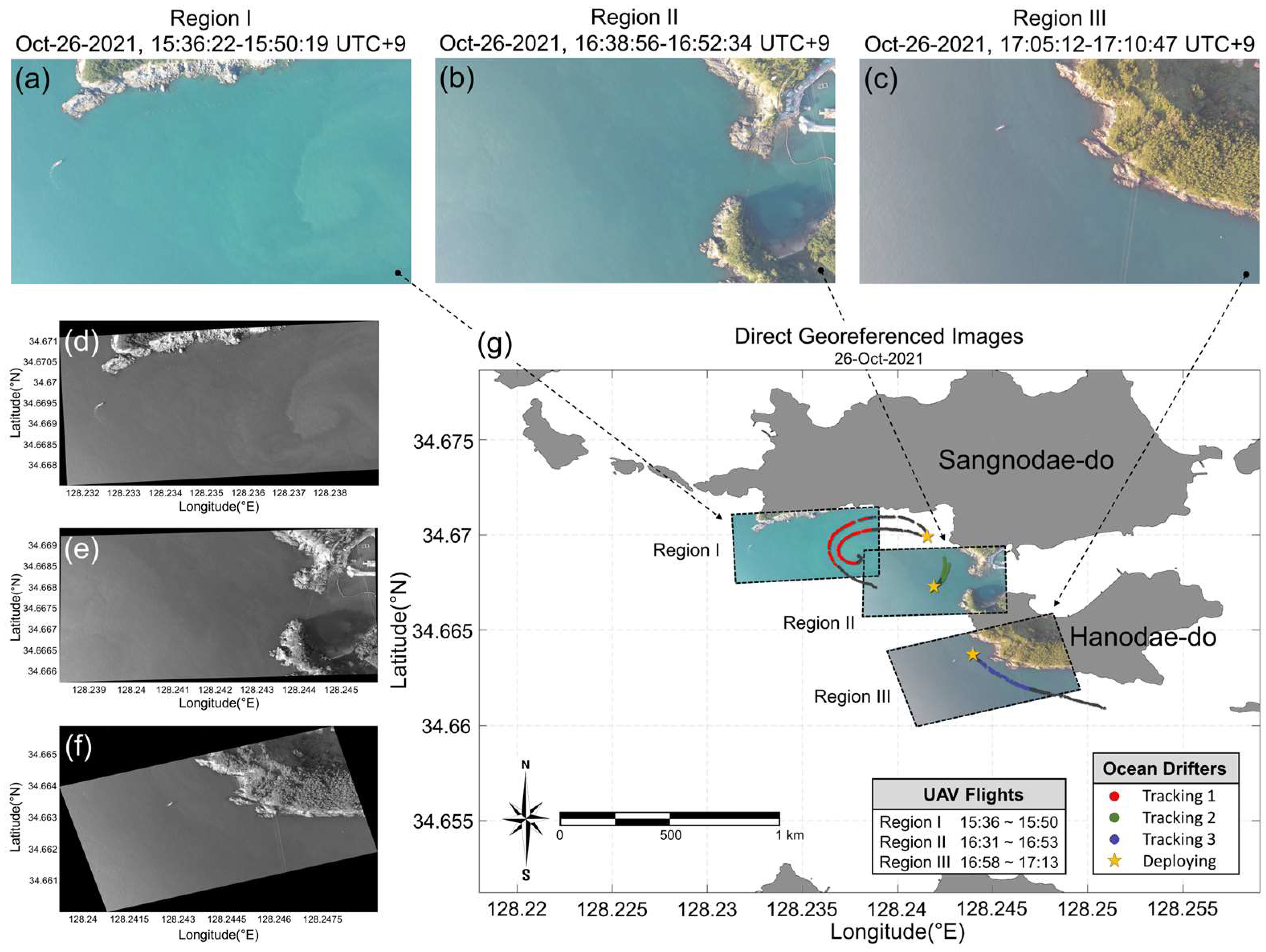
2.1. Study Area

Nodae-do is an island in Tongyeong-si, Gyeongsangnam-do, which is off the Southern coast of South Korea. The coast is characterized by rias, which have a large number of islands and contribute to a complex coastline (Figure 1a); the flow pattern also shows complex aspects. The sea bottom slope is generally uneven at a relatively shallow depth of approximately 50 m, and the change in the flow environment is great, owing to the interaction between currents and the seafloor. The size of the Nodae-do is approximately 3.7 km in width and 2.1 km in length, and it is divided into two sections with a distance of approximately 100–200 m, being divided into two regions, namely Sangnodae-do (upper section) and Hanodae-do (lower section) (Figure 1b). The coast near Nodae-do features relatively shallow water depths of 5–15 m and several surrounding islands (Figure 1c); therefore, the water is channeled between the islands, and the current encounters a shallow coastal seabed and becomes barotropically unstable, starts to swirl, and produces numerous small-scale eddies. The friction between the seabed and ocean currents generates suspended sediments, which rise to the sea surface and move along the ocean currents, thereby allowing visual identification of ocean currents with distinct optical properties.

2.2. In Situ Data

UAV Observations were conducted on 26 October 2021, around the southwest coast of Nodae-do, which features numerous capes with complex coastlines that extend diagonally. Three coastal areas with various current characteristics were selected for observation, and the raw UAV images of each Region I-III are shown in Figure 2a–c. The UAV aerial images were sampled with 1 Hz using a DJI Mavic Air 2 quadcopter equipped with a self-stabilized 3-axis gimbaled 1/2.3″ CMOS sensor. Using 4 K resolution (3840 × 2160) video recordings at an altitude of 500 m, high-resolution observational data with a ground sample distance (GSD) of approximately 20 cm were obtained. The video data were acquired while maintaining a nadir shooting angle with the self-stabilized UAV hovering at the same location at an altitude of approximately 500 m above the three areas where the drifters were released. The UAV flew through each area for approximately 10–15 min, during which raw images were recorded. The position and attitude information of the UAV, including pitch, roll, and yaw, were recorded by a built-in global positioning system (GPS) and inertial motion unit (IMU) sensor modules.

Two drifters were used in the UAV observation area to validate the ocean current estimations (Figure 3a). Drifters were designed to minimize wind resistance by reducing exposure above the sea surface. For buoyancy, the body was encapsulated with a float, and, below this, a 70 cm length crossed polyvinyl chloride (PVC) drogue was installed to operate primarily by ocean currents during deployment (Figure 3b). The drifters were hand-dropped after the sea surface was sufficiently stabilized to exclude the disturbance of waves caused by the movements of the ship in the UAV observation area. Information related to the location and movement of the drifter, sampled at 0.1 Hz, was recorded and transmitted in real-time by an Iridium satellite communicating with a GPS module mounted on the top of the body (Figure 3c). This functionality extended to both coastal and offshore areas. Raw GPS data were linearly interpolated to fill the data gaps generated by intermittent lost connections and moving-averaged by 2 min to minimize noise and bias. The accuracy of the GPS was estimated to be <2.5 m around the observation point [28].

2.3. UAV Image Processing

The overall workflow for the optical image-based submesoscale ocean dynamics estimation, divided into six subsequent steps, is shown in Figure 4. The images acquired from the UAV were sampled at a frame rate of 1 Hz and georeferenced directly to the geographic coordinates for pixel quantification. Additional preprocessing with image registration was conducted to correct errors caused by UAV drift. FA-MEMD was used to decompose mixed multicomponent images into distinct 2D oscillatory patterns or structures characterized by different spatial frequencies, known as BIMFs. Subsequently, these BIMFs were reconstructed to represent surface waves and currents. Finally, each oceanic process was analyzed independently. Fourier analysis was used to identify the period and directionality of the surface waves, and Optical Flow was used to retrieve the vector field of the surface current.

For spatial analysis of UAV imagery observed in the ocean, each aerial image must be projected onto the water surface (geographic coordinates) using georeferencing. In ocean observations, unlike the availability of fixed ground control points (GCPs) on land, stable reference points are constrained by the fluctuating nature of the sea surface and difficulty in identifying distinctive features. Therefore, direct georeferencing was used to calculate the collinearity equation based on the rotation matrix shown in Equation (1). This method directly connects the pixel coordinate system of the observed aerial images to the water surface coordinate system using image metadata recorded by the onboard GPS/IMU sensor modules of the UAV without the need for ground information [29]. The rotation matrix for the projection between the two coordinate systems was calculated based on the posture information (roll ($\varnothing$), pitch ($\theta$), and yaw ($\phi$) (RPY)).

$$\begin{array}{c}\mathrm{R}\mathrm{P}\mathrm{Y}=\left[\begin{array}{ccc}cos\varnothing & -sin\varnothing & 0\\ sin\varnothing & cos\varnothing & 0\\ 0& 0& 1\end{array}\right]\left[\begin{array}{ccc}cos\theta & 0& sin\theta \\ 0& 1& 0\\ -sin\theta & 0& cos\theta \end{array}\right]\left[\begin{array}{ccc}1& 0& 0\\ 0& cos\phi & -sin\phi \\ 0& sin\phi & cos\phi \end{array}\right]\\ =\left[\begin{array}{ccc}cos\varnothing cos\theta & cos\varnothing sin\theta sin\phi -sin\varnothing cos\phi & cos\varnothing sin\theta cos\mathsf{\phi }+sin\varnothing cos\phi \\ sin\varnothing cos\theta & sin\varnothing sin\theta sin\phi +cos\varnothing cos\phi & sin\varnothing sin\theta cos\mathsf{\phi }-cos\varnothing cos\phi \\ -sin\theta & cos\theta sin\phi & cos\theta cos\phi \end{array}\right]\end{array}$$

(1)

Next, the actual distance per pixel was calculated using geometric information (longitude, latitude, and altitude) and internal camera variables (CCD sensor size, focal length, and angle of view). Based on the calculated projection angle (RPY) and proportion, every aerial image was georectified to create a planimetrically corrected image sequence for Geographic Information System (GIS) analysis. In Figure 2d–g, we allocated the WGS84 geographic coordinates to every pixel in the aerial images using direct georeferencing and overlaid the images on the map to verify the consistency of the coastline and quantify the physical variables of the sea surface. Projection directly onto the water surface was limited because the elevation of the sea surface could not be calculated on the projected coordinate system. To consider the rough surface of the actual sea, we assumed the sea surface to be flat so that the elevation differences caused by the wave height within the observation range could be disregarded [30].

The precision of the GPS/IMU sensor module for the self-stabilization function of UAVs, which is crucial for acquiring consistent images from UAVs flying over a designated point in the study area, is directly associated with the optical processing quality. Although the hover-flying function of the latest UAV models has an error of centimeters, the influences of external environmental factors (generally the wind-induced drift and tilt of the UAV) inevitably distort the consistency of an image captured at several hundred meters in height, which in turn affects the results of the sea surface current measurement. Therefore, rather than limiting the wind environment to reconstruct the sea surface current, as in previous studies [31,32], we aligned the frames through image processing and compensated for biases in the GPS/IMU sensor module induced by instantly occurring wind. The Features from Accelerated Segment Test (FAST) algorithm was adopted to identify ideally repeatable points with high local information content, with a primary emphasis on land within the image sequences [33]. Subsequently, a corresponding relationship was established between these points, and all subsequent images were matched using an affine transformation. All images were subsequently processed into a grayscale image for improved visualization.

In sea surface observation imagery, optical signals such as waves, currents, sun-glints, and water properties are mixed [16]. This implies that the acquired data can be a consequence of multiple physical phenomena that interact with each other at different scales [21]. To properly interpret UAV images, it is essential to perform a signal analysis that distinguishes and extracts only the features of desirous phenomena, such as surface waves and currents, from these multiple signals. Conventional signal processing methods, such as the Fourier Transform and Wavelet Analysis, are appropriate for repetitive and standardized periodic signals. They analyze the signals with respect to either the time or frequency domain using predefined mathematical functions and assuming a fixed basis for decomposition [34,35]. In contrast, EMD is a data-driven signal processing algorithm that has been established to be able to perfectly analyze nonlinear and nonstationary data by obtaining local features and time-frequency distribution of the data [24]. This adaptability to signal variability makes it a suitable algorithm for processing complex and diverse nonlinear signals. Recently, this method has been applied in the fluid mechanics research community, and its performance quality has been proven [21,36,37,38,39,40].

In this study, we used the FA-MEMD method, an extended version of EMD specifically designed for multidimensional data processing. Temporal sea surface images were used to account for depicting the spatial changes or variations over time and decomposed into a finite number of BIMFs and a residual component. BIMFs represent bidimensional components capturing spatial patterns or structures in both the horizontal and vertical dimensions of the data, with each BIMF corresponding to a different scale or frequency in the bidimensional signal. The FA-MEMD method uses order statistic filtering instead of spline interpolation during the sifting process, thereby enabling scale-based decomposition for large datasets [24]. This approach effectively addresses the computational costs associated with expanding the data domain, thereby facilitating fast and adaptive multidimensional signal processing [21]. Furthermore, it maintains scale alignment among the BIMFs throughout the dimensional domain of the input data. It also corrects discontinuous biases using a noise-assisted extension, making it advantageous for spatial analysis [41]. The aforementioned benefits of FA-MEMD render it well suited for decomposing extensive and nonlinear sea surface time-series from UAV-obtained images.

Each aerial image obtained from the three different experimental sites was reorganized into a three-dimensional spatiotemporal dataset, enabling the desired underlying oceanic process characteristic determination. The entire dataset was enveloped to account for variations in the brightness values across the image set over time. A Region of Interest (ROI) was selected for each scene, focusing on areas with distinct optical signatures for surface currents to minimize mode mixing and consider computational efficiency when applying FA-MEMD: 1500 × 1500 pixels, 1000 × 1000 pixels, and 500 × 1700 pixel domains for each region.

We used the Optical Flow (OF) algorithm, a computer vision technique that analyzes the patterns of individual pixel brightness changes between consecutive images to represent motion vectors and quantify the motion of sea surface currents. The OF algorithm computes 2D velocity components based on pixel displacements across the entire image domain and the known time interval between frames. The algorithm assumes that the pixel intensity remains invariant, such that the time derivative of the image intensity can be accurately evaluated under the hypothesis that the pixel displacement is sufficiently small, such that the pixel intensity remains nearly constant [42,43,44].

We used Optical Flow Algorithm for Particle Image Velocimetry, OFAPIV, an open-source MATLAB (R2007a or later versions) program developed by Liu [45], to estimate the sea surface currents from the UAV images. This hybrid method, which combines the Optical Flow method with the cross-correlation method, yields consistently improved results compared with other velocity measurement techniques [45]. OFAPIV has been widely adopted and validated in previous studies involving various images of fluid flows, clouds, and oceans [46,47,48,49,50,51,52]. Specifically designed for estimating motion from high-resolution, continuous image patterns, this tool excels in accurate identification and feature tracking, making it invaluable for fluid dynamics and oceanographic research.

Various flow visualization techniques require observable features in images for vector estimation, such as tracers (particles, dyes, and foam), or variations in the specific physical properties of the water body, such as differences in chlorophyll or light reflection [15,53,54]. In this study, we used turbid water, distinguished from the surroundings by a high concentration of suspended particulate matter, as tracers to analyze the movement of surface currents. To facilitate turbid water detection and improve accuracy, we corrected the scene illumination and improved visibility by applying Contrast Limited Adaptive Histogram Equalization (CLAHE) before applying the Optical Flow method [17,43]. CLAHE is a type of histogram equalization technique that is particularly effective in addressing the problem of uneven or non-uniform illumination across an image by limiting the amplification of contrast [55,56]. Consequently, it enhances the details of the suspended matter, making it easy to identify and, in turn, analyze relevant optical signatures.

We subsequently applied the OFAPIV method to the ROIs of the three regions and extracted high-resolution velocity fields with a spatial resolution of 1 m per pixel. Depending on the current velocities of each region, the time interval of the input data was set to 2 s so that the pixel displacements between frames were sufficiently noticeable (between 1 and 5 pixels) for vector estimation. The physics-based Optical Flow equation in image coordinates is abbreviated as per a previous study [45].

The parameters and subroutines used in the algorithm were configured according to the values suggested in previous studies [45,52,57]. The Lagrange multipliers act like a diffusion coefficient in the corresponding Euler–Lagrange equations and are responsible for smoothing out finer flow structures; they were set to the typical computational values of 20 and 2000 for the Horn–Schunck and the Liu–Shen estimators, respectively. The scale factor for the downsampling of raw images was set to 0.5 to handle large pixel displacements (e.g., >10 pixels) and improve the computation accuracy, and the number of iterations for image warping was set to 1. Additionally, the Gaussian filter size used for correcting local illumination intensity changes was set to 300 pixels, depending on the characteristic length scale of the local change patterns. To eliminate small random noise, it was set to 1 pixel because the noise was removed during the image decomposition stage.

3. Results

3.1. Sea Surface Signal Decomposition

Surface wave and current movements were distinguished from the UAV images using FA-MEMD. The decomposition results are listed from high-to low-frequency modes as BIMF1 to the residual images (Figure 5a). Unlike Fourier Transform and Wavelet Analysis, EMD does not show serious energy leakage problems in the vicinity of frequencies of interest. Therefore, when all mode signals are combined, the original signal can be synthesized as it is [58]. Before recombining the BIMFs and classifying them into components for waves and currents, a Hilbert Spectral Analysis (HSA) was conducted to identify the frequency characteristics of each BIMF. Because a direct extension of the scale quantification method for multiple dimension data has not yet been developed, we applied HSA to time-series data extracted from the BIMF sequences.

In Figure 5b, the normalized marginal spectra of the BIMFs are arranged by frequency in the same order as the mode number. The peak positions of BIMF1 to BIMF3 were distributed in the range of 0.15–0.35 Hz, while those from BIMF4 to BIMF7 were located within the range of 0–0.05 Hz. Based on the typical classification criteria of ocean wave spectrum according to wave period, and considering the shallow coastal topography in the study area, the peak of the BIMFs located over 0.1 Hz were recombined and divided into a relatively high-frequency wave signal. These signals encompass wind-driven ordinary gravity waves with periods of 1–30 s (i.e., wave frequency f = 0.03–1 Hz) [59]. Low-frequency signals and a residual component corresponding to the surface current signal were also reaggregated to clarify the estimation target in Section 3.3.

Figure 6b,c,e,f,h,i show reconstructed wave and current signals in the three study areas of Figure 6a,d,g. In Figure 6b,e,h, the propagating wave pattern with distinctly repetitive cycles can be seen, and Figure 6c,f,i show the movement of the water mass caused by distinct turbidity due to the suspended matter generated by friction with the seabed.

3.2. Surface Wave Signal Analysis

The reconstructed wave signals, listed sequentially from high to low frequency, were analyzed by applying a Fourier analysis, resulting in a 2D wavenumber spectrum E(K_x, K_y). We confirmed the distinct characteristics of each wave mode, including wavelength and wave direction, in the spatial and wavenumber domains. Figure 7 shows BIMF1 to BIMF3 of Region I listed in order of high to low wave frequency. The highest frequency wave signal, BIMF1, demonstrated wavenumbers, K_x, K_y, ranging from approximately 0.03 to 0.1 radm⁻¹ (i.e., 7–24 m wavelength). Accordingly, BIMF2 displayed K_x, K_y ≈ 0.02–0.05 radm⁻¹ (i.e., 14–35 m wavelength), and BIMF3 exhibited K_x, K_y ≈ 0.01–0.03 radm⁻¹ (i.e., 24–70 m wavelength). Notably, as the wavelength increased, the peaks concentrated toward the center (0, 0). The northeastward wave propagation, represented by the peak location of approximately 45° N in all the wave signals, agreed with the visual inspection of the UAV images observed. The three wave mode frequencies (from BIMF1 to BIMF3) showing the peak of the marginal spectrum in order at f = 0.34, 0.18, and 0.16 Hz (i.e., 2.94, 5.55, and 6.25 s period) are discussed in Figure 5b.

In addition, we could conclude that the wave that appeared in Figure 7 is a shallow water wave driven by the wind. According to the shallow water wave equation, the phase speed is about 7.00–12.12 ms⁻¹ with 5–15 m of water depth and a gravitational acceleration of 9.8 ms⁻². For validation, we estimated the phase speed from the X-T (Hovmöller) diagram from modes 1 to 3, accounting for 7.95 ms⁻¹, 8.87 ms⁻¹, and 9.57 ms⁻¹, respectively.

Wave observations using stereo-optical and X-band radar can estimate the wave height and calculate the 3D wave spectrum [60,61]. However, since the single digital camera on a UAV has limitations in retrieving the wave height, we only described the wave characteristics such as wave number, wavelength, and celerity. Also, since this study focuses on a data-driven nonlinear ocean signal decomposition method, EMD and Optical Flow were used instead of FFT, which is generally used for 3D wave spectral analysis.

The results of this submesoscale gravity wave analysis emphasized the potential for conducting independent wave analyses based on the frequency of sea surface UAV-observed images.

3.3. Optically Derived Surface Current

The surface current vector was calculated by applying the OF algorithm to only the wave-excluded current signal to improve the estimation accuracy. Vorticity contour plots are also displayed for improved eddy visualization. The results of the surface current estimation for the three study areas are presented in chronological order.

Region I was captured on 26 October 2021 at 15:36 UTC+9 for approximately 14 min in the shallow coastal area below Sangnodae-do, and part of the eddy-like swirling pattern of approximately 500 m can be seen in high-resolution UAV images (Figure 8a). A complex counterclockwise swirling flow pattern generated by a suspended matter entrained by the advection was identified. Consecutive flights made between 16:00 and 16:30 UTC+9 showed that the eddy traveled in the same southeast direction, increasing in size according to the southeasterly falling tides flowing through Sangnodae-do.

The same counterclockwise surface current was identified in the vector field estimated using the OF algorithm and matched well with the UAV image (Figure 8b). The eddy had a diameter of approximately 250 m and a maximum speed of 0.15–0.17 ms⁻¹ at the periphery, approximately 50 m away from the eddy center. The mean current speed was 0.13 ms⁻¹, and the current direction is shown in Figure 8c. The surface current vorticity exhibited specific eddy-like features in agreement with visual inspection of the optical images, reaching a peak of 0.004 s⁻¹ at the eddy center (Figure 8d). The strong velocity gradient between the high speed of the eddy periphery and the close-to-zero speed of the eddy core indicates the nonlinear dynamics of the eddy. This submesoscale eddy seems to have been created by the barotropic instability of the horizontal current shear, encountering a topographic obstacle (protrusions) located in the upper left side of Sangnodae-do, which can be seen in the image (Figure 8a).

Region II was captured right after Region I on 26 October 2021, 16:38 UTC+9, for approximately 14 min. The video was recorded above the narrow channel between Sangnodae-do and Hanodae-do, the right side of the Region I eddy feature (Figure 3). A similar fraction of the counterclockwise swirling pattern was observed from the lower left side of the images. The surface current showed a northeastern flow toward the coast of Sangnodae-do.

The estimated surface current direction also described the features of the counterclockwise eddy within the image. It showed flow characteristics curved in the order of northeast–northwest, with a rather uniform direction (Figure 9a). The magnitude of the surface current was high for the visually observed features in Figure 9b, with a strong turbidity gradient region. Compared to the first region, the surface current magnitude was slightly slower, with an average of 0.1 ms⁻¹ (Figure 9c). The vorticity map exhibiting a positive area (approximately 0.002 s⁻¹) at the left boundary of the image indicated the existence of a counterclockwise eddy that was not observed owing to the image cut-off (Figure 9d).

Region III was acquired below the previous Region II (Figure 10a), the coastal area of Hanodae-do, on 26 October 2021 at 17:05 UTC+9 for approximately 5 min. This area had a tidal residual flow at ebb tide, passing along the complex coastline of Hanodae-do at a relatively high speed compared to the former two areas. This residual flow is expected to be the major outflow current generating the eddy of the previous scenes, and it can be assumed that the translational motion of the eddy was in the same direction as this flow toward the southeast.

Figure 10a presents the ROI of this experiment site. The outflowing residual current was clearly observed in the resulting surface current map (Figure 10b). The current speed of approximately 0.35 ms⁻¹ was generally directed east, with some meandering features describing the motion of the surface currents (Figure 10c). The surface current vorticity did not exhibit any specific features, such as eddies, because there were no vortex patterns in the optical images of this area (Figure 10d).

3.4. Ocean Drifter Validation

The optically estimated surface current was validated using drifters deployed in each study area during UAV observation. The zonal (U) and meridional (V) velocity components and magnitudes are compared individually in Figure 11. The scatter plots show the flow characteristics of each study area (Figure 2a–c). The positive and negative values of the U and V components indicate the different flow directions of the two drifters.

In Region I, the surface current speed of approximately 0.2 ms⁻¹ showed a pattern of increasing and decreasing gradually with time and was not constant. This is attributable to the change in the speed of the drifters as they move away and approach the eddy center (Figure 11, sky blue-colored dot). In Region II, the scatters, concentrated in the center, indicate the weaker surface current having relatively less variability with a value between 0.08–0.12 ms⁻¹ compared with Region I (Figure 11, blue-colored dot). Unlike the other scenes, the amount of data in Region III was much smaller. This occurred because the deployed drifters moved out of the fixed image frame of the UAV too quickly, as the surface current in the area was nearly three times faster (0.3 ms⁻¹) than in the previous region (Figure 11, navy-colored dot).

The R² values for the U and V components of the surface current were 0.92 and 0.88, respectively, and we validated the practical estimation of approximately 90% of the variance in the surface current compared to the drifter data (Figure 11a,b). The root mean square error (RMSE) for the U and V components across all three regions was 0.02 and 0.03 ms⁻¹, respectively, demonstrating high-accuracy results in estimation. The V component showed a relatively large RMSE compared with U, which is likely an error caused by the dominance of the zonal sea surface current flow. The R² and RMSE values of total velocity magnitude also showed good accuracy and agreement with 0.80 and 0.03 ms⁻¹, respectively (Figure 11c).

The efficacy of the Optical Flow algorithm depends on its ability to discern and appropriately handle optical noise within the images. In the context of this study, the notable presence of surface waves has a discernible impact on the vector estimation results of sea surface currents. This effect stems from the optical characteristics associated with surface waves, necessitating careful consideration of their effects on the algorithm performance.

Figure 12 presents a comparative analysis of the sea surface current estimations, illustrating the results before and after removing the wave signal. This comparative study serves as a pivotal step in elucidating the consequences of retaining or eliminating wave signals on the accuracy and reliability of vector estimation. In Figure 12a, when the wave signal was not removed, the vector field exhibited noticeable interference, particularly aligning with the direction of the northeastward propagating waves, indicating the influence of the surface wave features. In contrast, Figure 12b shows the same counterclockwise rotating vector field as the visually inspected flow pattern of the input image.

The observations from this comparative analysis underscore the importance of effectively addressing surface waves when using an Optical Flow algorithm. Removing the wave signal significantly improves the accuracy and fidelity of sea surface current vector estimations by mitigating the disturbances induced by propagating waves. These findings provide valuable insights into the refinement of methodologies for Optical Flow algorithms in the context of oceanographic studies, emphasizing the need for tailored approaches to handle dynamic light motion and shadows in UAV images for robust and accurate vector estimation.

4. Discussion

4.1. Direct Georeferencing

In the context of the geometric correction of remote sensing data, the accuracy of quantifying physical variables is intricately tied to the precision of the recorded metadata. Although land-based georeferencing benefits from numerous fixed reference points, allowing for effective post-processing with GCPs and achieving centimeter-level precision, sea surfaces pose unique challenges. The dynamic and ever-changing nature of the ocean limits the availability of fixed points, complicating the efforts to supplement errors in GPS/IMU sensor data. In such environments, ensuring projection consistency is a critical concern, potentially compromising the accuracy of direct georeferencing.

A pragmatic approach was used to overcome these challenges. Assuming that images were captured at the designated point in the air while the UAV was flying, a representative set of metadata values was determined and uniformly applied to all images. This strategy aimed to mitigate sensor-related errors in image projection and enhance the overall georeferencing consistency.

Despite these efforts, the discussion acknowledged the ongoing need for advancements in georeferencing methodologies specific to ocean observations. This included improvements in GPS/IMU sensors and the exploration of alternative approaches, such as using UAVs equipped with real-time kinematics (RTKs) to overcome the inherent challenges of the ocean environment.

4.2. Effect of Land Signals on Image Decomposition

The FA-MEMD method has been proven effective in decomposing sea surface images in this study, and addressing certain limitations that may impact its performance is essential. One notable challenge with the FA-MEMD method is its sensitivity to unwanted standout signals such as land and coastal boundaries. When applied to datasets covering both terrestrial and oceanic regions, the accuracy of the method decreases because of abrupt transitions between these distinct environments, resulting in spurious modes in the decomposition results. These spurious modes may not correspond to meaningful components of the signal but can emerge because of the adaptability of EMD to local variations. Rapid shifts in pixel values in the images can overshadow the actual local extrema (maxima and minima), making it difficult to identify true turning points in the images during the sifting process. Consequently, discontinuities in the BIMF components do not accurately capture the underlying components of the signal, thereby affecting the interpretability of the decomposition and the reliability of the method in such regions.

In ocean remote sensing, it is common to mask land areas to eliminate the impact of the ground, which has higher optical properties than the ocean. However, because these masked areas in the image can also introduce signal discontinuities, we addressed this issue by adjusting the ROI. The coastal ground in the images was excluded, and only the ocean area was set as the ROI to focus solely on the target sea surface signals.

4.3. Parameters Setting for FA-MEMD

The FA-MEMD is a powerful technique for signal decomposition. However, certain parameters must be considered in order to decompose the surface waves and currents and obtain satisfactory results. We referred to the guidelines for parameter settings included in the FA-MEMD algorithm [21]. Because the parameters used in FA-MEMD are data-driven values, users must test an appropriate value within the suggested range.

In this study, the parameters were chosen to balance between allowing for sufficient decomposition of waves and currents within the image while not demanding excessively long computation times. The maximum number of modes (i.e., a certain number of iterations for the sifting process) was limited to seven for calculation efficiency. The window size determined the distance between the extrema and played a crucial role in adjusting the characteristic scales of the modes. Through extrema detection of physical oscillations, considering the scale of the surface wave signal, the window size was chosen from the data (making EMD ‘data-driven’) and was set to six. The sifting tolerance was set to 10, approximately 0.1% of the signal amplitude referred to in a previous study [21], which led to good results and avoided oversifting, balancing factors such as the signal-to-noise ratio, preservation of fine details, computational efficiency, and accuracy.

In addition, repeated experiments are necessary to accumulate a sufficient dataset and establish a statistical standard for parameter settings when decomposing UAV-based sea surface imagery.

4.4. Computataional Resources

Although FA-MEMD has been implemented using various strategies for fast and adaptive calculations, processing the entire image area obtained from the UAV remains a computationally intensive task. The ability of FA-MEMD to handle multidimensional data contributes to its effectiveness but also leads to increased computational complexity. As a result, the method may face limitations in processing extensive datasets within reasonable timeframes, particularly when dealing with real-time or near-real-time applications.

In this study, the computational burden of FA-MEMD was managed to a certain extent by adjusting the size of the ROI to 1500 × 1500 pixels for Region I, 1000 × 1000 pixels for Region II, and 500 × 1700 pixels for Region III while partially dividing the time-series of the input data.

Advancements in memory capacity and computational technology are expected to alleviate these challenges. Continued efforts to optimize the algorithms and leverage parallel processing techniques may further enhance the computational efficiency of this method, making it accessible for broader applications in oceanographic research.

4.5. Surface Current Estimation

The OF algorithm identifies optical features in images and estimates motion vectors by tracking changes in pixel brightness across image sequences. In this study, suspended sediments in the coastal regions created distinct fronts between clear waters, enabling the OF algorithm to recognize and discern features for surface current estimation. However, in the case of clear water that lacks discernible current indicators, proper current estimation is challenging. Similarly, when observing the sea surface, the performance of the OF algorithm may be indirectly influenced by weather conditions, including the direct distortion of surface waves, as discussed in Section 3.4. Optical noise, such as sun-glints or cloud reflections on the sea surface, can also contaminate images, potentially reducing image quality or introducing unnecessary light changes, narrowing the valid image area, and further diminishing algorithm accuracy.

To address these issues, we recorded our UAV video under conditions of clear sunny skies to exclude the effects of clouds reflected from the sea surface. To minimize the effect of the sun-glints and maximize the available image areas, we adjusted the direction of the UAV to shoot with its back to the sun and chose the ROIs with less contaminated areas. Controlling these dynamic light and shadow interferences poses a substantial challenge for velocimetry algorithms.

5. Conclusions

Submesoscale physical processes, decomposed into surface waves and currents, were analyzed and estimated individually from UAV images taken from off the coastal area of Nodae-do, South Sea, Korea. Observations were made when sufficient suspended matter was mixed with clear water to create a surface turbidity gradient. Assisted by visible optical properties, the detailed structure of the submesoscale dynamics was observed several times using a UAV over the southern bay of the island. The following conclusions were drawn for each process.

• The UAV imagery was decomposed into several BIMFs using FA-MEMD, demonstrating its proficiency in processing nonlinear spatiotemporal data. The surface wave and current signal were distinguished based on the frequency (0.1 Hz) for each mode obtained using HSA.
• Wave characteristics, including the wavelength and wave direction, were spatially analyzed using a 2D FFT. From BIMF1 to BIMF3, wind-driven surface waves propagating northeastward with high-frequency (wavenumbers, K_x, K_y of 0.02–0.1 m⁻¹) signals can be seen in the order of short to long wavelengths. Each wave of various scales that were mixed was confirmed.
• The surface current was estimated using an open-source OF algorithm, which is widely adopted to calculate motion vectors from consecutive sea surface images. The optically derived current field from the sum of BIMF4 to the residual showed flow patterns consistent with the in situ drifter deployment. The current velocities throughout the three observation scenes exhibited reasonable validation results with R² and RMSE values of 0.804 and 0.033 ms⁻¹, respectively.

Based on these results, we demonstrated the feasibility of UAV-based submesoscale investigations in the ocean. Eddy dynamics with a diameter of approximately 250 m and 0.15–0.17 m s⁻¹ velocity observed in coastal environments were reproduced and discussed. The proposed framework for decomposing the imagery into sea surface waves and currents can be applied to various image processing studies in the oceanographic field. Furthermore, our findings contribute to unresolved submesoscale ocean dynamics.

References

1. McWilliams, J.C. Submesoscale currents in the ocean. Proc. R. Soc. A Math. Phys. Eng. Sci. 2016, 472, 2189. [Google Scholar] [CrossRef]
2. Taylor, J.R.; Thompson, A.F. Submesoscale Dynamics in the Upper Ocean. Annu. Rev. Fluid Mech. 2023, 55, 103–127. [Google Scholar] [CrossRef]
3. Chelton, D.B.; Schlax, M.G.; Samelson, R.M. Global observations of nonlinear mesoscale eddies. Prog. Oceanogr. 2011, 91, 167–216. [Google Scholar] [CrossRef]
4. Morrow, R.; Le Traon, P.Y. Recent advances in observing mesoscale ocean dynamics with satellite altimetry. Adv. Space Res. 2012, 50, 1062–1076. [Google Scholar] [CrossRef]
5. Capet, X.; Campos, E.J.; Paiva, A.M. Submesoscale activity over the Argentinian shelf. Geophys. Res. Lett. 2008, 35, L15605. [Google Scholar] [CrossRef]
6. Garabato, A.C.N.; Yu, X.; Callies, J.; Barkan, R.; Polzin, K.L.; Frajka-Williams, E.E.; Griffies, S.M. Kinetic Energy Transfers between Mesoscale and Submesoscale Motions in the Open Ocean’s Upper Layers. J. Phys. Oceanogr. 2022, 52, 75–97. [Google Scholar] [CrossRef]
7. Ferrari, R.; Wunsch, C. Ocean Circulation Kinetic Energy: Reservoirs, Sources, and Sinks. Annu. Rev. Fluid Mech. 2009, 41, 253–282. [Google Scholar] [CrossRef]
8. Wang, Q.; Pang, C.; Dong, C. Role of submesoscale processes in the isopycnal mixing associated with subthermocline eddies in the Philippine Sea. Deep-Sea Res. II Top. Stud. Oceanogr. 2022, 202, 105148. [Google Scholar] [CrossRef]
9. Haine, T.W.N.; Marshall, J. Gravitational, Symmetric, and Baroclinic Instability of the Ocean Mixed Layer. J. Phys. Oceanogr. 1998, 28, 634–658. [Google Scholar] [CrossRef]
10. Boccaletti, G.; Ferrari, R.; Fox-Kemper, B. Mixed Layer Instabilities and Restratification. J. Phys. Oceanogr. 2007, 37, 2228–2250. [Google Scholar] [CrossRef]
11. Lévy, M.; Ferrari, R.; Franks, P.J.S.; Martin, A.P.; Rivière, P. Bringing physics to life at the submesoscale. Geophys. Res. Lett. 2012, 3, 1–13. [Google Scholar] [CrossRef]
12. Mahadevan, A. The Impact of Submesoscale Physics on Primary Productivity of Plankton. Annu. Rev. Mar. Sci. 2016, 8, 161–184. [Google Scholar] [CrossRef]
13. Thomas, L.N.; Tandon, A.; Mahadevan, A. Submesoscale processes and dynamics. Ocean. Model. Eddying Regime Geophys. Monogr. Ser. 2008, 177, 17–38. [Google Scholar]
14. Yurovsky, Y.Y.; Kubryakov, A.A.; Plotnikov, E.V.; Lishaev, P.N. Submesoscale Currents from UAV: An Experiment over Small-Scale Eddies in the Coastal Black Sea. Remote Sens. 2022, 14, 3364. [Google Scholar] [CrossRef]
15. Anderson, D.; Bak, A.S.; Brodie, K.L.; Cohn, N.; Holman, R.A.; Stanley, J. Quantifying Optically Derived Two-Dimensional Wave-Averaged Currents in the Surf Zone. Remote Sens. 2021, 13, 690. [Google Scholar] [CrossRef]
16. Dérian, P.; Almar, R. Wavelet-Based Optical Flow Estimation of Instant Surface Currents from Shore-Based and UAV Videos. IEEE Trans. Geosci. Remote Sens. 2017, 55, 5790–5797. [Google Scholar] [CrossRef]
17. Rodríguez-Padilla, I.; Castelle, B.; Marieu, V.; Bonneton, P.; Mouragues, A.; Martins, K.; Morichon, D. Wave-Filtered Surf Zone Circulation under High-Energy Waves Derived from Video-Based Optical Systems. Remote Sens. 2021, 13, 1874. [Google Scholar] [CrossRef]
18. Castro, S.L.; Emery, W.J.; Wick, G.A.; Tandy, W. Submesoscale Sea Surface Temperature Variability from UAV and Satellite Measurements. Remote Sens. 2017, 9, 1089. [Google Scholar] [CrossRef]
19. Yurovsky, Y.Y.; Kudryavtsev, V.N.; Grodsky, S.A.; Chapron, B. Validation of Doppler Scatterometer Concepts using Measurements from the Black Sea Research Platform. In Proceedings of the “2018 Doppler Oceanography from Space (DOfS)” Workshop, Brest, France, 10–12 October 2018; IEEE: Washington, DC, USA, 2018. [Google Scholar]
20. Kubryakov, A.A.; Lishaev, P.N.; Chepyzhenko, A.I.; Aleskerova, A.A.; Kubryakova, E.A.; Medvedeva, A.V.; Stanichny, S.V. Impact of Submesoscale Eddies on the Transport of Suspended Matter in the Coastal Zone of Crimea Based on Drone, Satellite, and In Situ Measurement Data. Oceanology 2021, 61, 159–172. [Google Scholar] [CrossRef]
21. Thirumalaisamy, M.R.; Ansell, P.J. Fast and Adaptive Empirical Mode Decomposition for Multidimensional, Multivariate Signals. IEEE Signal Process. Lett. 2018, 25, 1550–1554. [Google Scholar] [CrossRef]
22. Huang, N.E.; Shen, Z.; Long, S.R.; Wu, M.C.; Shih, H.H.; Zheng, Q.; Liu, H.H. The empirical mode decomposition and the Hilbert spectrum for nonlinear and non-stationary time series analysis. Proc. R. Soc. A Math. Phys. Eng. Sci. 1998, 454, 903–995. [Google Scholar] [CrossRef]
23. Nunes, J.C.; Bouaoune, Y.; Delechelle, E.; Niang, O.; Bunel, P. Image analysis by bidimensional empirical mode decomposition. Image Vis. Comput. 2003, 21, 1019–1026. [Google Scholar] [CrossRef]
24. Bhuiyan, S.M.; Adhami, R.R.; Khan, J.F. Fast and Adaptive Bidimensional Empirical Mode Decomposition Using Order-Statistics Filter Based Envelope Estimation. EURASIP J. Adv. Signal Process. 2008, 2008, 18. [Google Scholar] [CrossRef]
25. Chen, C.Y.; Guo, S.M.; Chang, W.S.; Tsai, S.H.; Cheng, K.S. An improved bidimensional empirical mode decomposition: A mean approach for fast decomposition. Signal Process. 2014, 98, 344–358. [Google Scholar] [CrossRef]
26. Riffi, J.; Mahraz, A.M.; Abbad, A.; Tairi, H. 3D extension of the fast and adaptive bidimensional empirical mode decomposition. Multidimens. Syst. Signal Process. 2015, 26, 823–834. [Google Scholar] [CrossRef]
27. He, Z.; Li, J.; Liu, L.; Shen, Y. Three-dimensional empirical mode decomposition (TEMD): A fast approach motivated by separable filters. Signal Process. 2017, 131, 307–319. [Google Scholar] [CrossRef]
28. Jung, D.; Lee, J.S.; Baek, J.Y.; Nam, J.; Jo, Y.H.; Song, K.M.; Cheong, Y.I. High Temporal and Spatial Resolutions of Sea Surface Current from Low-Altitude Remote Sensing. J. Coast. Res. 2019, 90, 282–288. [Google Scholar] [CrossRef]
29. Mian, O.; Lutes, J.; Lipa, G.; Hutton, J.J.; Gavelle, E.; Borghini, S. Direct georeferencing on small unmanned aerial platforms for improved reliability and accuracy of mapping without the need for ground control points. Int. Arch. Photogramm. Remote Sens. Spat. Inf. Sci. 2015, 40, 397. [Google Scholar] [CrossRef]
30. Lee, J.S.; Baek, J.Y.; Shin, J.; Kim, J.S.; Jo, Y.H. Suspended Sediment Concentration Estimation along Turbid Water Outflow Using a Multispectral Camera on an Unmanned Aerial Vehicle. Remote Sens. 2023, 15, 5540. [Google Scholar] [CrossRef]
31. Streßer, M.; Carrasco, R.; Horstmann, J. Video-Based Estimation of Surface Currents Using a Low-Cost Quadcopter. IEEE Geosci. Remote Sens. Lett. 2017, 14, 2027–2031. [Google Scholar] [CrossRef]
32. Horstmann, J.; Streßer, M.; Carrasco, R. Surface currents retrieved from airborne video. In Proceedings of the OCEANS 2017, Aberdeen, UK, 19–22 June 2017; pp. 1–4. [Google Scholar]
33. Rosten, E.; Drummond, T. Machine Learning for High-Speed Corner Detection. In Proceedings of the Computer Vision—ECCV 2006, Graz, Austria, 7–13 May 2006; pp. 430–443. [Google Scholar]
34. Rai, V.K.; Mohanty, A.R. Bearing fault diagnosis using FFT of intrinsic mode functions in Hilbert–Huang transform. Mech. Syst. Signal Process. 2007, 21, 2607–2615. [Google Scholar] [CrossRef]
35. Mercorelli, P. A denoising procedure using wavelet packets for instantaneous detection of pantograph oscillations. Mech. Syst. Signal Process. 2013, 35, 137–149. [Google Scholar] [CrossRef]
36. Dahl, M. Turbulent Statistics from Time-Resolved PIV Measurements of a Jet Using Empirical Mode Decomposition. In Proceedings of the 18th AIAA/CEAS Aeroacoustics, Colorado Springs, CO, USA, 4–6 June 2012. [Google Scholar]
37. Ansell, P.J.; Balajewicz, M.J. Separation of Unsteady Scales in a Mixing Layer Using Empirical Mode Decomposition. AIAA J. 2017, 55, 419–434. [Google Scholar] [CrossRef]
38. Ansell, P.J.; Mulleners, K. Multiscale Vortex Characteristics of Dynamic Stall from Empirical Mode Decomposition. AIAA J. 2020, 58, 600–617. [Google Scholar] [CrossRef]
39. Koll, M.; Favale, J.; Kirchner, B.M.; Elliott, G.S.; Dutton, J.C. Flow Structure Identification in the Near Wake of an Axisymmetric Supersonic Base Flow Using MEEMD. In Proceedings of the 47th AIAA Fluid Dynamics, Denver, CO, USA, 5–9 June 2017. [Google Scholar]
40. Koll, M.; Scott, A.; Elliott, G.S.; Dutton, J.C. Flow Structure Identification in the Near Wake of a Supersonic Separated Flow Using FAEMD. In Proceedings of the 2018 Fluid Dynamics, Atlanta, GA, USA, 25–29 June 2018; p. 3540. [Google Scholar]
41. Ur Rehman, N.; Mandic, D.P. Filter Bank Property of Multivariate Empirical Mode Decomposition. IEEE Trans. Signal Process. 2011, 59, 2421–2426. [Google Scholar] [CrossRef]
42. Horn, B.K.; Schunck, B.G. Determining optical flow. Artif. Intell. 1981, 17, 185–203. [Google Scholar] [CrossRef]
43. Liu, T.; Wang, B.; Choi, D.S. Flow structures of Jupiter’s Great Red Spot extracted by using optical flow method. Phys. Fluids 2012, 24, 096601. [Google Scholar] [CrossRef]
44. Tu, Z.; Van Der Aa, N.; Van Gemeren, C.; Veltkamp, R.C. A combined post-filtering method to improve accuracy of variational optical flow estimation. Pattern Recognit. 2014, 47, 1926–1940. [Google Scholar] [CrossRef]
45. Liu, T.; Salazar, D.M. OpenOpticalFlow_PIV: An Open Source Program Integrating Optical Flow Method with Cross-Correlation Method for Particle Image Velocimetry. J. Open Res. Softw. 2021, 9, 3. [Google Scholar] [CrossRef]
46. Quénot, G.M.; Pakleza, J.; Kowalewski, T.A. Particle image velocimetry with optical flow. Exp. Fluids 1998, 25, 177–189. [Google Scholar] [CrossRef]
47. Corpetti, T.; Mémin, E.; Pérez, P. Dense estimation of fluid flows. IEEE Trans. Pattern Anal. Mach. Intell. 2002, 24, 365–380. [Google Scholar] [CrossRef]
48. Corpetti, T.; Heitz, D.; Arroyo, G.; Mémin, E.; Santa-Cruz, A. Fluid experimental flow estimation based on an optical-flow scheme. Exp. Fluids 2006, 40, 80–97. [Google Scholar] [CrossRef]
49. Ruhnau, P.; Kohlberger, T.; Schnörr, C.; Nobach, H. Variational optical flow estimation for particle image velocimetry. Exp. Fluids 2004, 38, 21–32. [Google Scholar] [CrossRef]
50. Liu, T.; Shen, L. Fluid flow and optical flow. J. Fluid Mech. 2008, 614, 253–291. [Google Scholar] [CrossRef]
51. Heitz, D.; Héas, P.; Mémin, E.; Carlier, J. Dynamic consistent correlation-variational approach for robust optical flow estimation. Exp. Fluids 2008, 45, 595–608. [Google Scholar] [CrossRef]
52. Heitz, D.; Mémin, E.; Schnörr, C. Variational fluid flow measurements from image sequences: Synopsis and perspectives. Exp. Fluids 2009, 48, 369–393. [Google Scholar] [CrossRef]
53. Liu, T. OpenOpticalFlow: An Open Source Program for Extraction of Velocity Fields from Flow Visualization Images. J. Open Res. Softw. 2017, 5, 29. [Google Scholar] [CrossRef]
54. Cao, Y.; Wu, Y.; Yao, Q.; Yu, J.; Hou, D.; Wu, Z.; Wang, Z. River Surface Velocity Estimation Using Optical Flow Velocimetry Improved with Attention Mechanism and Position Encoding. IEEE Sens. J. 2022, 22, 16533–16544. [Google Scholar] [CrossRef]
55. Zuiderveld, K. Contrast Limited Adaptive Histogram Equalization. In Graphic Gems IV; Academic Press: Cambridge, MA, USA, 1994; pp. 474–485. [Google Scholar]
56. Vidhya, G.R.; Ramesh, H. Effectiveness of Contrast Limited Adaptive Histogram Equalization Technique on Multispectral Satellite Imagery. In Proceedings of the international Conference on Video and Image Processing, Beijing, China, 17–20 September 2017; pp. 234–239. [Google Scholar]
57. Liu, T.; Merat, A.; Makhmalbaf, M.H.M.; Fajardo, C.; Merati, P. Comparison between optical flow and cross-correlation methods for extraction of velocity fields from particle images. Exp. Fluids 2015, 56, 166. [Google Scholar] [CrossRef]
58. Yang, W.; Tavner, P.J. Empirical mode decomposition, an adaptive approach for interpreting shaft vibratory signals of large rotating machinery. J. Sound Vib. 2009, 321, 1144–1170. [Google Scholar] [CrossRef]
59. Munk, W.H. Origin and generation of waves. In Proceedings of the 1st International Conference on Coastal Engineering, Long Beach, CA, USA, 1 January 1950; ASCE: Reston, VI, USA, 1950; pp. 1–4. [Google Scholar]
60. Guimarães, P.V.; Ardhuin, F.; Bergamasco, F.; Leckler, F.; Filipot, J.F.; Shim, J.S.; Dulov, V.; Benetazzo, A. A data set of sea surface stereo images to resolve space-time wave fields. Sci. Data 2020, 7, 145. [Google Scholar] [CrossRef] [PubMed]
61. Benetazzo, A.; Serafino, F.; Bergamasco, F.; Ludeno, G.; Ardhuin, F.; Sutherland, P.; Sclavo, M.; Barbariol, F. Stereo imaging and X-band radar wave data fusion: An assessment. Ocean Eng. 2018, 152, 346–352. [Google Scholar] [CrossRef]
Figure 1. (a) Study area located off the coast of South Sea of Korea with a rias coast. (b) The red box in (a) indicates the survey area, Nodae-do, with a group of islands around. (c) Three-dimensional bathymetric contour map of the study area.
Remotesensing 16 02275 g001
Figure 2. Raw images of the study area obtained from the unmanned aerial vehicle (UAV) in the three regions I, II, and III. (a) The south coast of Sangnodae-do, (b) between Sangnodae-do and Hanodae-do, and (c) the southern coast of Hanodae-do. The tidal currents flowing around the islands interact with these complex shallow coastal regions and resuspend sediments and particulate matter in the water near the coast, allowing visual water movement observation. (df) Direct georeferenced images in the same order as regions I-III. (g) Projected and overlapped direct georeferenced images on the WGS84 coordinate map, with a UAV flight time of three study areas and ocean drifter trajectories.
Remotesensing 16 02275 g002
Figure 3. (a) Ocean drifters deployed in the observation area. (b) Structure of the drifter (body, float, drogue). (c) Iridium communication satellite 9602-LP global positioning system (GPS) module in the body of the drifter.
Remotesensing 16 02275 g003
Figure 4. Overview of the unmanned aerial vehicle (UAV) data processing steps to analyze the sea surface waves and currents.
Remotesensing 16 02275 g004
Figure 5. (a) Seven decomposed Bidimensional Intrinsic Mode Functions (BIMFs) and a residual of Region I using Fast and Adaptive Multidimensional Empirical Mode Decomposition (FA-MEMD). (b) The marginal spectrum of Hilbert Spectral Analysis (HSA) results of each BIMF, arranged by frequency in the time and frequency domain. The Hilbert energy value was normalized in the range of 0–1 for an improved interpretation of peak location.
Remotesensing 16 02275 g005
Figure 6. (ac) Region I, Region of Interest (ROI) size with 1500 × 1500 pixels; (df) Region II, ROI size with 1000 × 1000 pixels; (gi) Region III, ROI size with 500 × 1700 pixels. Three regions are separated into two different ocean dynamics: surface waves containing periodic components and surface currents showing the detailed structure of turbid water.
Remotesensing 16 02275 g006
Figure 7. Fourier analysis results of surface wave signals for period and directionality. (a) BIMF1, (b) BIMF2, and (c) BIMF3 from Region I. The top panel: decomposed 300 m × 300 m wave component images with different wave features. The bottom panel: 2D wavenumber spectrum E(Kx, Ky). The wavenumbers, Kx, Ky are 2πn/dx in which n is the number of pixels and dx is the spatial scale of the unmanned aerial vehicle (UAV) images.
Remotesensing 16 02275 g007
Figure 8. Region I: (a) Estimated surface current location on the georeferenced image map with drifter trajectory. (b) Surface current vector map. (c) Surface current velocity map. (d) Surface current vorticity map.
Remotesensing 16 02275 g008
Figure 9. Region II: (a) Estimated surface current location on the georeferenced image map with drifter trajectory. (b) Surface current vector map. (c) Surface current velocity map. (d) Surface current vorticity map.
Remotesensing 16 02275 g009
Figure 10. Region III: (a) Estimated surface current location on the georeferenced image map with drifter trajectory. (b) Surface current vector map. (c) Surface current velocity map. (d) Surface current vorticity map.
Remotesensing 16 02275 g010
Figure 11. Comparison of surface current velocity magnitude from Optical Flow estimations and in situ drifters. (a,b) U and V components, and (c) velocity magnitude in total three areas (Region I-III). Optical and drifter velocities are moving-averaged by 1 and 2 min, respectively. The black dashed and solid lines denote the slope of the regression and the 1:1 line, respectively.
Remotesensing 16 02275 g011
Figure 12. (a) Original image of Region I obtained from the unmanned aerial vehicle (UAV). (b) Filtered image by eliminating the decomposed surface wave signal. The top panel: input image of the Optical Flow (OF) algorithm; the bottom panel: optically estimated current field. The effect of surface wave in estimating current is shown by the messy vector field in the bottom panel of the original image, disturbed by the northeastward propagating surface wave signal.
Remotesensing 16 02275 g012
Disclaimer/Publisher’s Note: The statements, opinions and data contained in all publications are solely those of the individual author(s) and contributor(s) and not of MDPI and/or the editor(s). MDPI and/or the editor(s) disclaim responsibility for any injury to people or property resulting from any ideas, methods, instructions or products referred to in the content.