Semantic Segmentation of Some Rock-Forming Mineral Thin Sections Using Deep Learning Algorithms: A Case Study from the Nikeiba Area, South Eastern Desert, Egypt

Abstract

Image semantic segmentation using deep learning algorithms plays a vital role in identifying different rock-forming minerals. In this paper, we employ the U-net model for its architecture that guarantees precise localization and efficient data utilization. We implement this deep learning model across two distinct datasets: (1) the first dataset from the ALEX Streckeisen website, and (2) the second dataset from the Gabal Nikeiba area, South Eastern Desert of Egypt. Our model exhibits excellent performance in both datasets, with an average accuracy of precision at 0.89 and 0.83, recall at 0.80 and 0.78, and F1 score at 0.82 and 0.79, respectively, helping in identifying and detecting rock-forming minerals in thin-section images. The model’s most exceptional performance is clearly in eleven different basement rock-forming minerals with precision up to 0.89, recall at 0.80, and F1 score at 0.82 on average. This study is significant as it represents the key to identifying and detecting minerals in the thin sections of rock samples in Egypt and the Arabian–Nubian Shield as a whole. By significantly reducing analysis time and improving accuracy compared to manual methods, it revolutionizes geological research and resource exploration in the region.

1. Introduction

On an image-thin section, mineral identification and textural description require microscopic investigation with interpretation and counting data obtained using a light microscope [1,2,3,4,5,6,7,8,9]. Petrography is a specialized discipline that involves extensive knowledge in identifying and classifying minerals and textural relationships within the rock [3]. According to the mineral compositions of the rocks, thin-section photos display color, grain size, shape, internal cleavage, structure, and other features [6,10]. These attributes offer valuable information on the petrographic properties of rocks. It is difficult to interpret some minerals in a rock-thin section, even for an experienced petrologist, since they are small, dark, or opaque. To identify minerals, other techniques may be used in addition to light microscopy, such as scanning electron microscopy (SEM) and electron probe microanalysis (EPMA), or bulk measurements, such as X-ray diffraction (XRD) [3].

As a result of point counting or grid-based statistics, workflows are used to deal with the massive amounts of data present in a single slide and accelerate the collection of representative quantitative data [3,6,11,12]. Despite being reliable and well-liked, this method skips over a lot of information on each image’s thin section or even entire thin sections in order to save time. This manual process requires a significant amount of time, money, and effort to complete. There are several approaches to categorizing information in an image using computer vision algorithms [3,13,14]. An algorithm that has seen a training set of photos is used to predict the class of a fresh observation using classification learning. A subfield of computer vision called semantic segmentation aims to identify the class label that each pixel in an image represents. In addition to autonomous vehicles [3,15], satellite image classification is another popular semantic segmentation approach [3,14,16,17]. These applications involve transforming pixels into meaningful output labels (e.g., boat, plane, car, road, person, tree, sky, etc.) as a result of extensive effort. Instance segmentation is a step further that seeks to group associated pixels into a region with a boundary, e.g., one quartz grain is distinct and separate from another. This study is not intended to address instance segmentation. However, using a “watershed” algorithmic approach as a post-processing step to an output image can still be suggested [3,18].

In the field of petrology, semantic segmentation is still in its infancy, while non-transferrable networks and small classification schemes for sandstones examine distinct objects from the organic petrology discipline [18,19,20]. Mlynarczuk and Skiba [21] demonstrate how this field is developing. Segmentation cannot be performed without a pixel-by-pixel label set [12]. With the purpose of labeling 2-dimensional RGB images captured by digital cameras linked to light microscope equipment, Shell Research developed Computer Aided Petrology (CAP) in the early- to mid-2000s. Through this method, a subject matter expert manually obtains an image.

Image segmentation plays a pivotal role in discriminating the mineral composition of rock units, particularly in the field of petrographic studies [22,23,24,25,26,27,28,29,30]. This process involves partitioning a digital image of a rock sample into multiple segments, each representing different minerals or textures. By applying machine learning algorithms, such as convolutional neural networks (CNNs), researchers can automate the identification and classification of these segments with high accuracy. These models are trained on datasets containing labeled images, enabling them to learn the unique features and patterns associated with various minerals [23,24,25,26]. Once trained, the machine learning models can analyze new rock images, segmenting and identifying mineral compositions quickly and efficiently. This approach not only enhances the precision of mineralogical analysis but also significantly reduces the time and effort required compared to traditional manual methods, thereby advancing the capabilities and scope of petrographic studies [23].

This study shows that the semantic segmentation of thin-section images from two datasets (dataset 1 with 10 images and dataset 2 with 5 images) can provide comprehensive scene understanding within a classification framework. Additionally, it can compute basic attributes much faster than an expert petrologist. In addition, experts may be able to gain some knowledge of all the thin sections while refining their interpretations of the primary, secondary, and accessory minerals—all of which are essential for refocusing their efforts on microscopy methods other than light microscopy.

Let us further assume that thin-section image analysis may yield additional quantitative geometric parameters (e.g., contact length, number of nearest neighbors, and preferred orientation). If so, a greater range of assessment models for applications in geomechanics and rock physics can be directly fed by these data. In order to achieve this, we train semantic segmentation models to extract classification information from 2D RGB images taken on the thin slices of basement rocks using the deep neural encoder–decoder architectures of U-net. An excellently hand-labeled collection of training photos is used to train this model. The following is the organization: First, we discuss the training dataset, the semantic segmentation networks, and the general effectiveness of the trained model to predict mineralogy using thin-section images. Next, we discuss the impact of the hyperparameters of the preferred model. Finally, we present a thorough statistical and petrological review of the preferred model, discuss limitations and opportunities, and present our conclusions.

One of the objectives of this study is to implement a novel deep learning image processing technique for the automatic identification of rock-forming mineral systems that help in creating detailed geological maps of the study area with high precision, as well as to investigate thin-section approaches that could help identify the minerals in the study area and their extension.

2. Materials and Methods

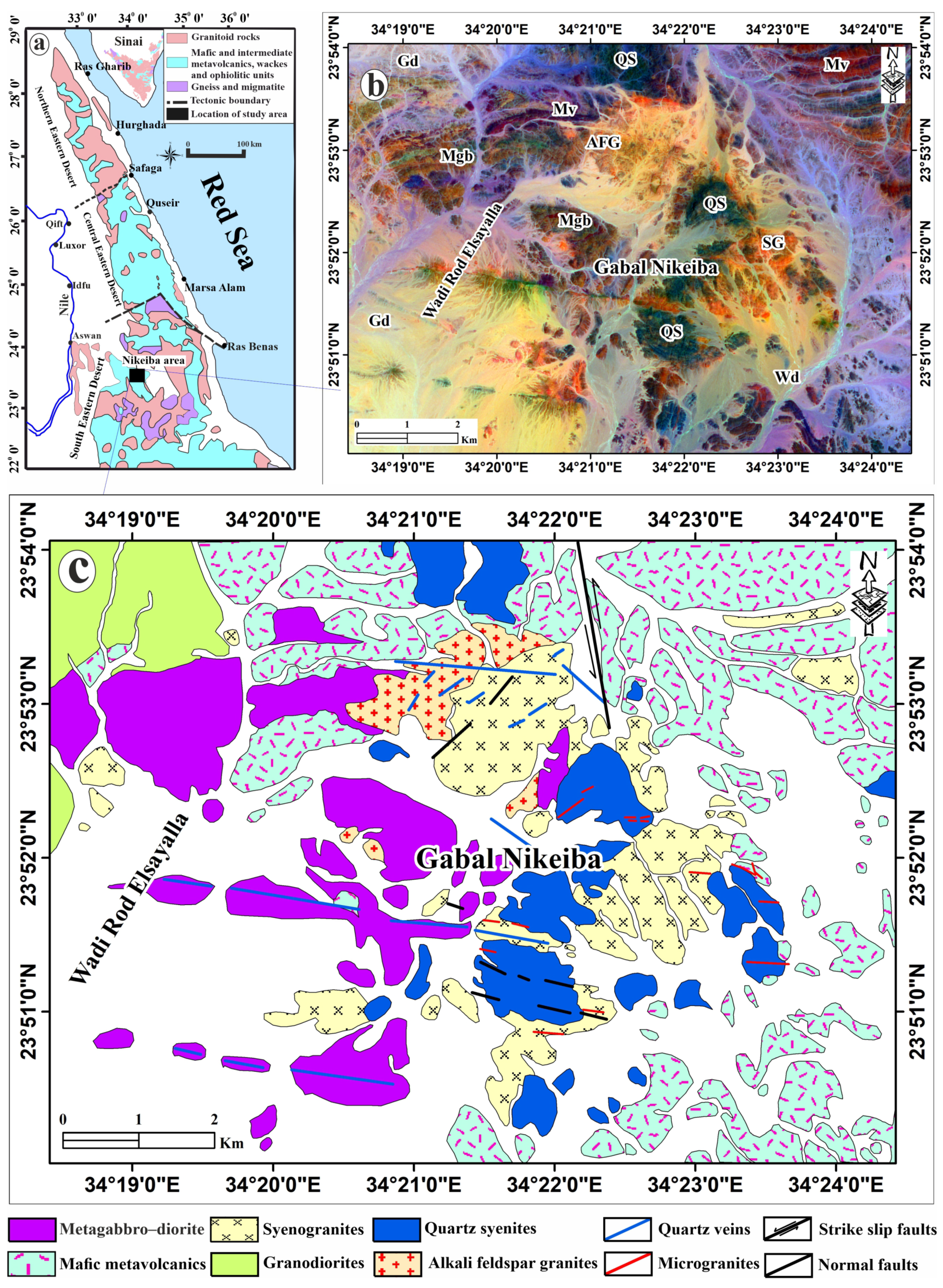
2.1. Geologic Setting and Petrography of the Study Area

The Nikeiba area belongs to the North Arabian–Nubian Shield (ANS) and is located in the South Eastern Desert of Egypt between latitudes 23°49′N to 23°53′N and longitudes 34°18′E to 34°24′E, with an area of ~416 km² (Figure 1). In this area, different types of lithological rocks are exposed including mafic metavolcanics, a metagabbro–diorite complex, granodiorites, syenogranites, alkali feldspar granites, and quartz syenites (Figure 2a–c). Many quartz veins dissect the above-mentioned units (Figure 2d) and microgranite dykes. These rock units are well discriminated using Sentinel-2 decorrelation stretch image (b12, b8, and b3 as RGB) (Figure 1b). Mafic metavolcanics and the metagabbro–diorite show intrusive contacts with granitic rocks. On the other hand, syenogranites show gradational contact with alkali feldspar granites. Many faults, mainly NW-SE, N-S, and E-W, dissect the area [31]. The proposed methods used in this paper are clearly shown in Figure 3. In this paper, we used two datasets (Figure 4 and Figure 5), which are described in detail in the following sections.

Syenogranites are pale pink to reddish-brown in color, and medium- to coarse-grained (Figure 2a). They are composed mainly of K-feldspar (55–60 vol.%), quartz (22–28 vol.%), plagioclase (10–15 vol.%), biotite (3–5 vol.%), muscovite (<1 vol.%), riebeckite, and arfvedsonite (Figure 5a–c). Chlorite and epidote are the main alteration minerals. Accessory minerals include zircon, apatite, beryl, and Fe-Ti oxides. Alkali feldspar granites are pink to red in color, and medium- to coarse-grained (Figure 2b). The main mineral constituents are K-feldspar (60–65%), quartz (24–30 vol.%), plagioclase (4–6 vol.%), biotite (~2 vol.%), riebeckite, and arfvedsonite (Figure 5d). Zircon, apatite, beryl, and opaque minerals are accessories, whereas chlorite and sericite are the alteration products of biotite and feldspar, respectively. Quartz syenites are medium- to coarse-grained and dark grey to pale pink in color (Figure 2c). Microscopically, they are composed of K-feldspar (65–70 vol.%), quartz (15–18 vol.%), sodic amphibole (arfvedsonite, riebeckite) (~6 vol.%), biotite (~4 vol.%), and accessory plagioclase (Figure 5e). Zircon, apatite, allanite, and opaque minerals are accessories. The alteration minerals of biotite and feldspar include chlorite and sericite, respectively (Figure 5e). For this study, we selected ten minerals that represent the different rock-forming minerals of the granitic rocks of the Nikeiba area. These minerals include primary magmatic minerals (quartz, K-feldspar, plagioclase, biotite, muscovite, and riebeckite–arfvedsonite), secondary minerals (chlorite), and accessory minerals “zircon and apatite”.

2.2. Image Datasets

In general, there are only a few label sets available for petrology. In order to create these sets and to compare several methods for automatic mineral identification in thin-section images, we produced a dataset with pixel-level segmentation masks for images containing various minerals. These datasets are divided into subgroups representing various mineralogical compositions. The datasets were gathered from two distinct sources: (1) the first dataset comprises high-resolution photographs from Alex Strekeisen’s website (https://www.alexstrekeisen.it); (2) the second dataset includes different granitic samples collected in the Nikeiba area, South Eastern Desert of Egypt. We prepared 24 thin sections from the specimens gathered in the Nikeiba area of Egypt’s Eastern Desert for microscopic analysis at the Geology Department of Kafrelsheikh University using a Kemet Geoform thin sectioning machine (Kemet International Ltd, Parkwood Trading Estate, Maidstone, United Kingdom). These sections were polished after being cut into billets, impregnated with white epoxy resin, mounted on glass slides, and ground to a final thickness of 30 μm. The process involved the careful polishing of the surface. The materials used included white epoxy (Resin A&B) and silicon carbide powder in various grit sizes: 220, 400, 600, 800, 1000, and 1200.

The petrographic analysis of the second dataset was conducted using an Olympus TH4-200 standard polarizing microscope equipped with a UC-30 digital camera [33,34]. Labeling images were taken using optical microscopes with 4× or 10× magnification, resulting in pixel resolutions ranging from 0.84 to 2.08 pixels/μm. The first dataset of Alex Strekeisen consists of 10 main minerals (

Table 1. Hyperparameters were tested for all base networks.

Hyperparameters	Spanned Range
Learn Rate Schedule	Piecewise
Learn Rate Drop	Period 2
Learn Rate Drop Factor	0.8
Initial Learn Rate	0.001
L2 Regularization	0.1
Max Epochs	75
Mini Batch Size	3
Shuffle	Every epoch

). Our second dataset from the granites of the Nikeiba area comprises ten different types of rock-forming minerals (Table 1). It is essential to emphasize that despite the fact that an experienced geologist can investigate many more minerals in a thin section, we only include 16 minerals in our work because gathering a huge collection of thin sections with the hand annotation of all the used minerals is resource-expensive.

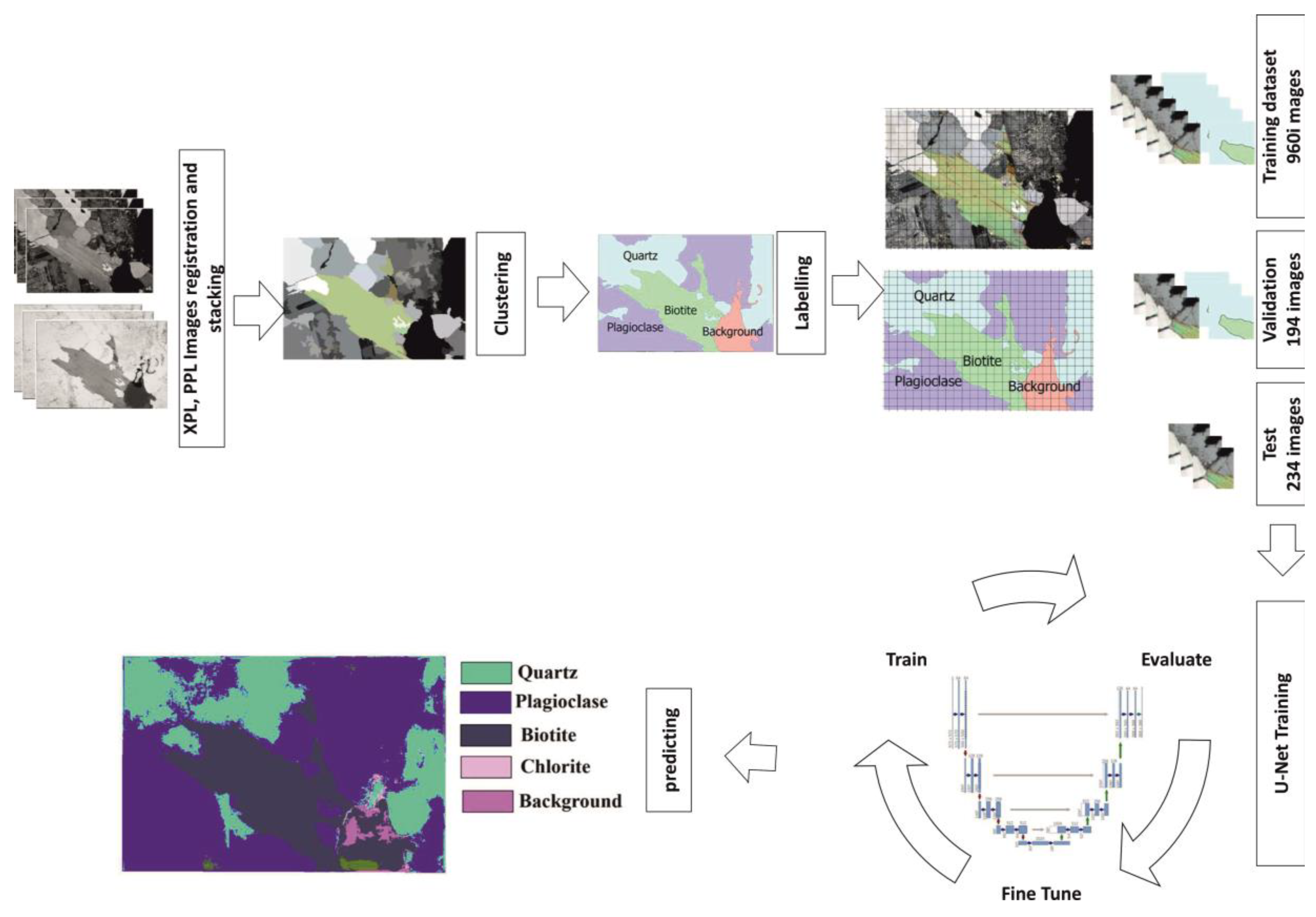
2.3. Preparing Thin-Section Samples for Deep Learning Analysis

The workflow of the methodology employed in this study is illustrated in Figure 3. Preparing thin-section training samples for deep learning in petrography requires a meticulous and technical approach. This begins with capturing images under two distinct lighting conditions: cross-polarized light (XPL) and Plane-polarized light (PPL) (Figure 4 and Figure 5). These imaging techniques are essential in petrography as they highlight different aspects of the mineral components in the thin sections. XPL and PPL images provide complementary information about the rock samples’ mineral composition, texture, and structure (Figure 4 and Figure 5). Obtaining high-quality and representative images under both lighting conditions is vital for the subsequent steps in the data preparation process.

Once the XPL and PPL images of the thin sections are obtained, the next critical step is image registration. This process involves adjusting and aligning the XPL and PPL images to match each other perfectly. Image registration is crucial as it ensures that the features observed in the XPL and PPL images correspond to the same areas of the thin section. Accurate alignment is essential for effectively combining data from both imaging modalities. This alignment allows for a more comprehensive analysis of the mineral components, combining the information obtained from both polarized light conditions.

After aligning the XPL and PPL images, they are stacked to form a single composite image. This composite image consists of six bands—three from the XPL image and three from the PPL image. Arranging the photos in this way forms a multi-dimensional dataset that captures the optical information from both types of polarized light. The next crucial step involves segmenting this stacked image (Figure 4 and Figure 5). This segmentation process isolates different regions within the image, facilitating the subsequent labeling process. By merging different segments under their respective labels, the process effectively categorizes various mineral components and other features in the thin sections. This step is fundamental in preparing the data for more detailed analysis and classification.

The final step in preparing the training samples involves two key activities: building a vector layer for labeling and tiling the stacked images (Figure 4 and Figure 5). The vector layer is meticulously constructed to label different mineral components within the sections. This layer includes major minerals and, importantly, mirror labels for secondary components (Figure 4 and Figure 5). This detailed labeling is vital for training deep learning algorithms to recognize and classify different minerals accurately. The last step is converting the stacked images and their corresponding vector layers into fixed-size square tiles. The tiles and their associated masks are input into a deep learning model like the U-net algorithm, which is commonly utilized for image segmentation. This method of dividing the images into tiles and applying masks is essential for effectively training deep learning models. It enables them to recognize and learn mineralogical characteristics in thin-section samples accurately.

2.3.1. Train, Validation, and Testing Datasets

In the labeled dataset, the images were randomly assigned to three subgroups: 960 images for training, 194 images for validation, and 234 images for testing. Every RGB image and its label are sized at 775 × 518 pixels. In this study, the model was initially fit using a training dataset with an optimized set of hyperparameters (Table 1) as the learning method [34]. Predicting the responses to the observations in the validation dataset was then accomplished using the fitted model. In the next phase, we tuned hyperparameters (Figure 4 and Figure 5) based on model performance against the validation dataset.

To perform semantic segmentation of thin-section images, we used a convolutional neural network based on a popular U-Net architecture (Figure 6) with batch normalization layers [35,36]. Adding residual connections inside convolution blocks increases learning speed and overcomes the vanishing gradient problem [37]. Using typical patch-based methodologies to train a neural network with uneven input will produce poor results. To address the issue of data imbalance, we applied a modified version of the specific data balancing strategy suggested by Kochkarev et al. [38]. Specifically, during the generation step, the patch probability maps that were based on the distance to the nearest class were replaced with the area of a certain class in the patch. Optimal hyperparameters for models based on Resnet-34 and the U-net network are listed in the right column.

2.3.2. CNN Architectures and Models

We applied semantic segmentation convolutional neural networks (CNNs) to classify each pixel in a thin-section image. This produces an image segmented according to the petrological class defined by the labeling schemes (16 classes). There are multiple types of networks for semantic segmentation, including ResNet34 and U-Net. All of these networks are effective and trainable, and they make use of the limited GPU resources available in the MATLAB libraries. Briefly, ResNet34 and U-Net include different network layers and have convolutional kernels of size 3 × 3, max pooling size 2 × 2, and a stride of two (Figure 6). ResNet 34 utilizes exactly the same 3 × 3 convolutional kernels, located at the beginning and end of the network. It makes connections between each of the two convolutional layers. Both base architectures include a softmax (probability) layer to get the highest probability pixel outcome from the classification procedure (Figure 6).

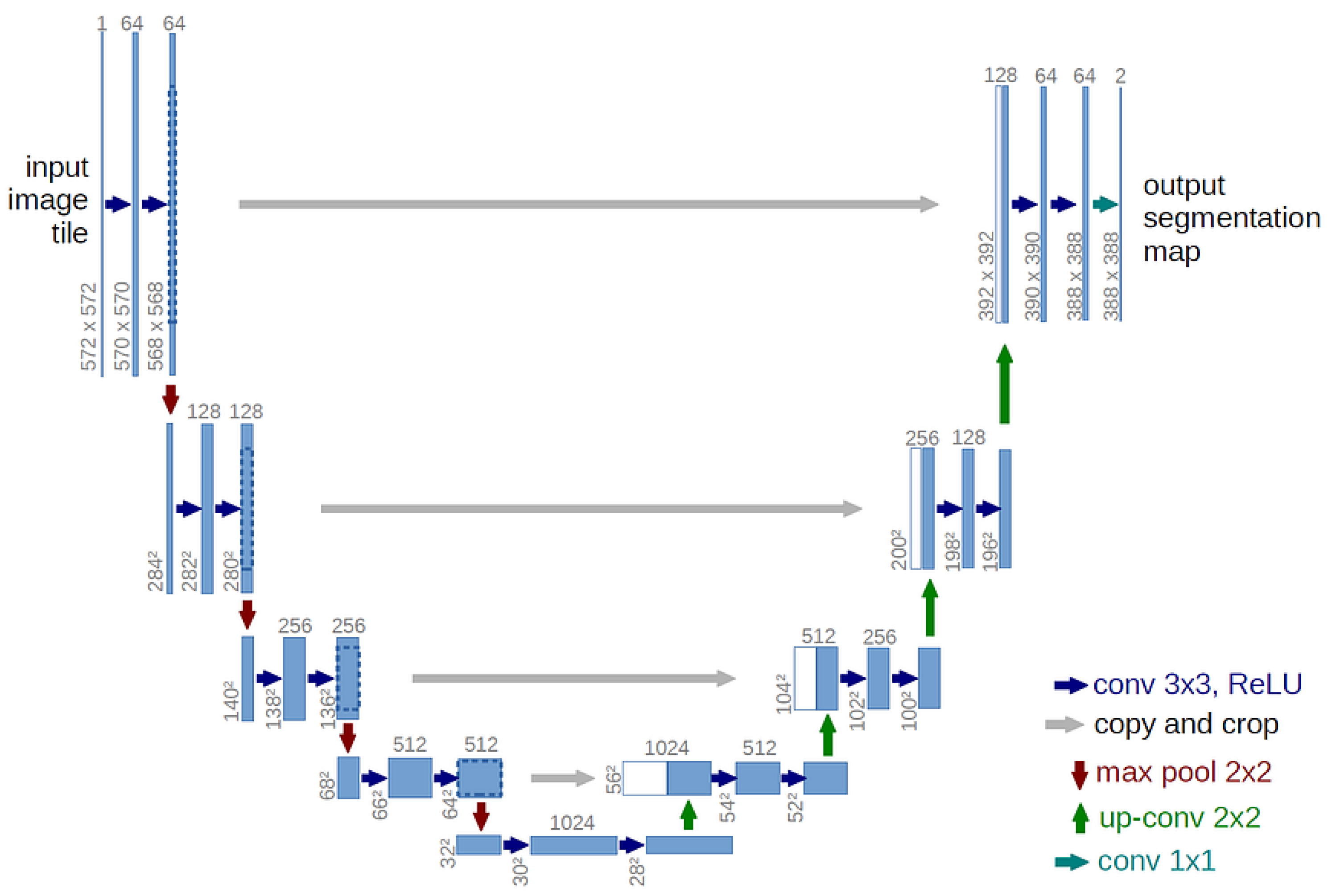
• Exploring the U-Net Architecture:  An Overview of its Structure for Efficient Image Segmentation U-Net is a convolutional neural network architecture developed primarily for biomedical image segmentation. This architecture is notable for its efficiency and accuracy in segmenting images, even with limited data. The structure of U-Net can be described in four main sections:

• Downsampling (Contracting Path): The first part of U-Net is the contracting path, which is a typical convolutional network. This path contains the continual application of two 3 × 3 convolutions (unpadded convolutions), each followed by a rectified linear unit (ReLU) and a 2 × 2 max pooling operation with stride 2 for downsampling. At each downsampling step, the number of feature channels is doubled. This part of the network captures the context in the input image, essential for accurate segmentation.
• Bottleneck: After several layers of downsampling, the U-Net reaches its bottleneck. This is the lowest level of the network, where it has the smallest spatial dimension of feature maps. In the bottleneck, two 3 × 3 convolutions are applied, followed by a ReLU. This section is crucial as it allows the network to process features at the lowest resolution, capturing the most abstract representations of the input data.
• Upsampling (Expanding Path): Following the bottleneck, the network then transitions into the expansive path, which includes a sequence of upsampling and convolution operations. The upsampling of the feature map is followed by a 2 × 2 convolution (“up-convolution”) that halves the number of feature channels. Then, a concatenation is performed with the correspondingly cropped feature map from the contracting path. This step is crucial for the network to learn precise localization, a critical aspect of accurate segmentation.
• Final Layer: The final layer of the network is a 1 × 1 convolution that maps each feature vector to the desired number of classes in the output segmentation map. This layer produces the final segmentation map, where each pixel in the image is classified into a specific class. The architecture’s use of expansive paths and concatenation with high-resolution features from the contracting path allows for precise localization and detailed segmentation.

3. Results and Discussion

3.1. Experiments Setup

In this paper, we conducted a series of experiments focusing on a subset of data, including image training datasets for three different types of mineral thin sections. These initial experiments were crucial for fine-tuning the various parameters we used in our study. To carry out these experiments, we employed the U-net deep learning model, which is renowned for its efficiency and accuracy in image segmentation tasks. The model was configured with specific parameters: a maximum of 20 epochs, a batch size of 8, and a learning rate tailored for optimal performance. Additional model arguments included settings for class balancing, mix-up, focal loss, and ignore classes, with a chip size set at 128 and the monitoring of the validation loss.

Further technical details of our experimental setup include the choice of RESNET34 as the backbone model, which is highly regarded for its performance in image classification tasks. We also utilized a pre-trained model to leverage previously learned patterns and features, enhancing the model’s effectiveness. The validation data comprised 10% of the total dataset, ensuring a robust evaluation of the model’s performance. An essential feature of our model training was the “STOP_TRAINING” functionality, which automatically halted training when no further improvements were observed, thereby optimizing the training process and preventing overfitting.

The entire configuration and adjustment of these specifications were carried out within the ArcGIS Pro version 3.0 environment, utilizing its deep learning toolbox. This environment provided a stable and efficient platform for manipulating the deep learning parameters and models, ensuring precise and reliable outcomes in our experiments. The integration of these advanced tools and settings in the ArcGIS Pro version 3.0 environment was crucial for achieving the high level of accuracy and efficiency required in our study of the mineral thin sections.

In our recent experiments, we focused on training data analysis using a balanced dataset, where 50% was allocated for validation and the other 50% for training [39]. This methodology was applied across 50 epochs to ensure comprehensive learning and evaluation. The results of these experiments were meticulously documented and presented in Figure 7, Figure 8 and Figure 9. Figure 7 offers a detailed look at the training and validation loss graph. This visual representation provides insights into the model’s performance over the course of the training process, highlighting the loss metrics during each epoch for both the training and validation phases.

3.2. Comparing the Two Datasets

A detailed overview of the model’s performance across various classes, with a focus on the precision, recall, and F1 score metrics, for the two datasets is shown in

Table 2. Evaluation matrix result for each class and the total average in the two datasets used.

The First Dataset from ALEX Strekeisen (https://www.alexstrekeisen.it)
Metrics	Quartz	Plagioclase	Biotite	Chlorite	Olivine	Serpentine	Tourmaline	Titanite	Talc	Background	Average
precision	0.81	0.78	0.90	0.89	0.87	0.88	1.00	0.78	0.94	0.92	0.89
recall	0.85	0.77	0.93	0.80	0.94	0.98	0.62	0.77	0.76	0.26	0.80
F1	0.83	0.78	0.91	0.84	0.91	0.93	0.77	0.77	0.84	0.40	0.82
The Second Dataset from the Gabal Nikeiba Area, South Eastern Desert, Egypt
Metrics	Quartz	Plagioclase	Biotite	K-feldspar	Riebeckite	Arfvedsonite	Muscovite	Apatite	Zircon	Background	Average
precision	0.91	0.81	0.77	0.91	0.95	0.84	0.79	0.92	0.76	0.68	0.83
recall	0.79	0.90	0.98	0.94	0.90	0.77	0.62	0.51	0.89	0.46	0.78
F1	0.84	0.85	0.86	0.92	0.92	0.80	0.69	0.66	0.82	0.55	0.79

.

• Quartz: The first dataset shows strong precision at 0.81 and recall at 0.85, leading to a balanced F1 score of 0.83, whereas the second dataset of the Gabal Nikeiba area displays excellent precision at 0.91 and recall (0.79) (Table 2), leading to a very high F1 score. This indicates a reliable performance in correctly identifying quartz and effectively reducing false negatives (Figure 8 and Figure 9).
• Plagioclase and Biotite: These minerals demonstrate high precision in the two datasets, ranging from 0.77 to 0.90, and recall from 0.77 to 0.98 (Table 2), suggesting the model’s strong capability in accurately identifying these minerals and consistently detecting their instances (Figure 8 and Figure 9).
• K-feldspar: In the Nikeiba area, it has strong precision (0.91) and recall (0.94), resulting in a very high F1 score (0.91) (Table 2). This result indicates that the model is very accurate in the detection of K-feldspar (Figure 9).
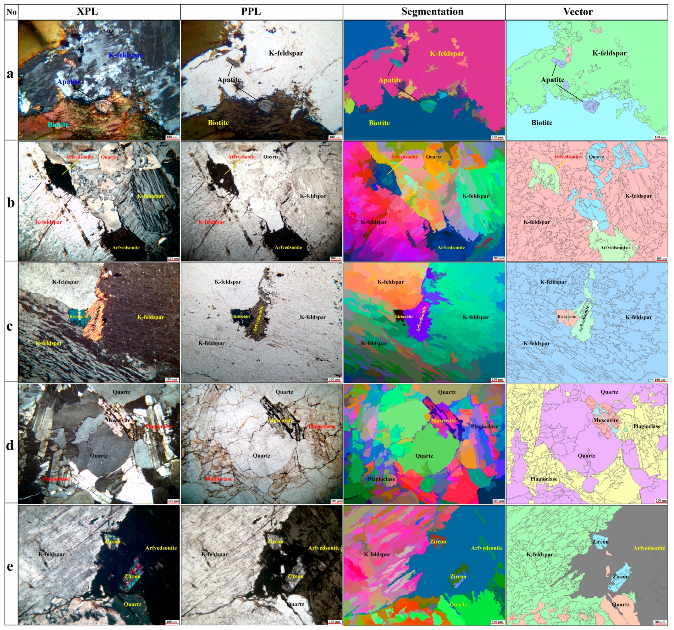
• Riebeckite and Arfvedsonite: These minerals belong to alkali amphibole and are present in the three different types of the Gabal Nikeiba granites (syenogranite, alkali feldspar granites, and quartz syenites) (Figure 5). They show a very high precision range from 0.84 to 0.95 and recall range from 0.77 to 0.90, leading to a strong F1 score of 0.80 and 0.92 (Table 2). This result exhibits the accuracy of the model in identifying and detecting these minerals (Figure 9).
• Muscovite: It shows moderate precision (0.79) and moderate recall (0.62), resulting in a moderate F1 score of 0.69 in the Nikeiba area, which implies the moderate performance of the model in both identifying and detecting the muscovite (Figure 9d).
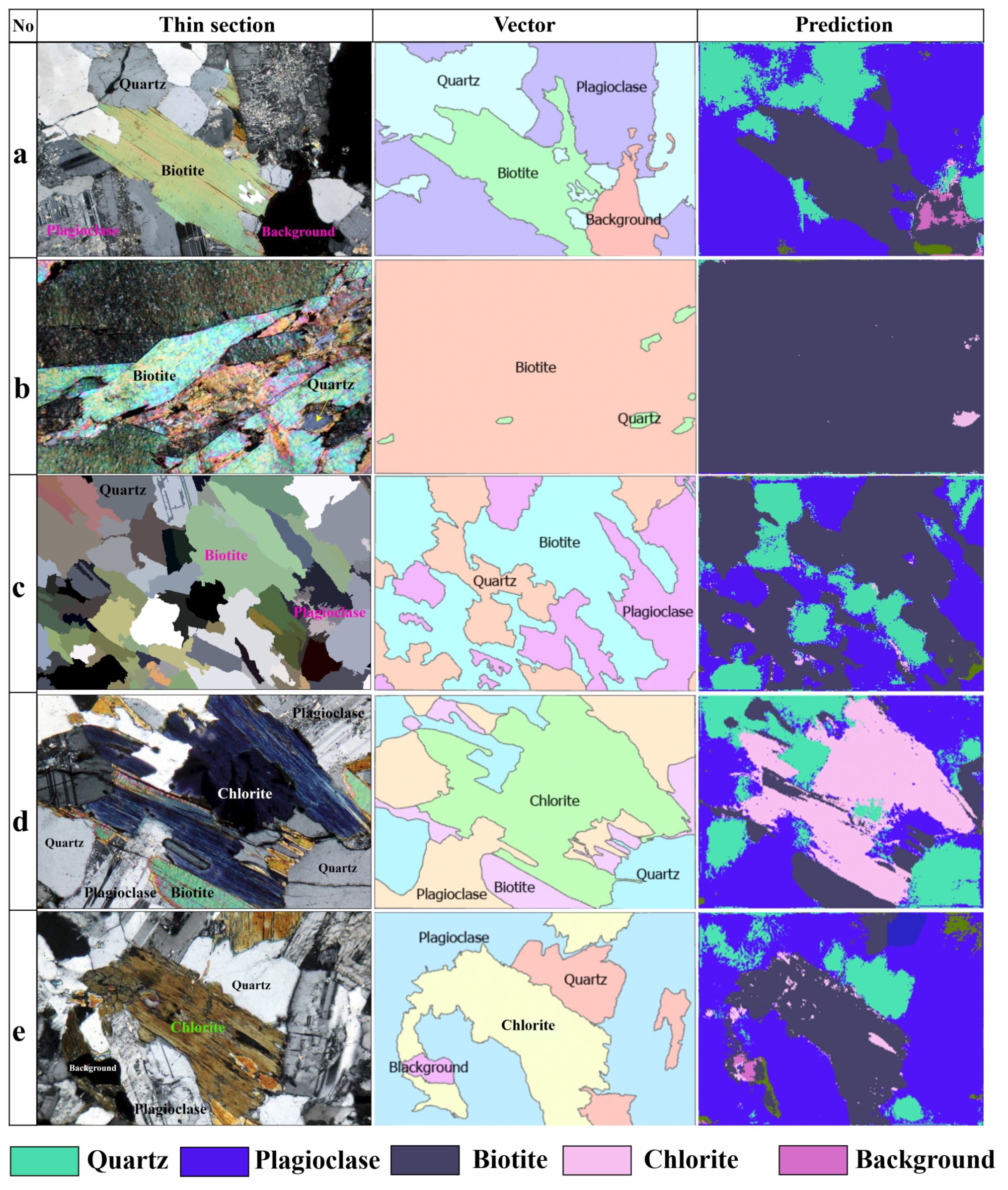
• Chlorite, Olivine, and Serpentine: These minerals run only in the first dataset, and they exhibit excellent precision ranging from 0.87 to 0.89 and recall from 0.80 to 0.98, resulting in a high F1 score of 0.84, 0.91, and 0.93, respectively (Table 2), indicating that the model shows exceptional performance in both accurately identifying and consistently detecting chlorite, olivine, and serpentine (Figure 8d–h).
• Titanite and Talc: These classes belong to the first dataset, and they have high precision (0.78 and 0.94, respectively; Table 2) but moderate recall (both at 0.77 and 0.76; Table 2), indicating the model’s effectiveness in correctly identifying them, though with some missed instances (Figure 8g–i).
• Tourmaline: It also runs in the first dataset and has perfect precision (1.00); its recall is significantly lower at 0.62, leading to an F1 score of 0.77 (Table 2). This suggests that while the model accurately identifies tourmaline, when it detects it, it misses a considerable number of instances (Figure 8j).
• Zircon: In the Nikeiba area, it is a prevalent accessory mineral (Figure 4e and Figure 8e). It has high precision (0.76) and strong recall (0.89), leading to a strong F1 score of 0.82 (Table 2). This indicates that the model accurately identifies and consistently detects the zircon (Figure 9e).
• Apatite: It is an accessory mineral in all the granitic phases of the Nikeiba area (Figure 4a). It has excellent precision (0.92) and low recall (0.51), leading to an F1 score of 0.66 (Table 2). This implies that the model accurately identifies and detects apatite with some missed instances (Figure 9a).
• Background: Notably, the model achieves a moderate to high precision range (0.68 to 0.92) in identifying the background in the two datasets but has a low recall (0.26 to 0.46, respectively), leading to a lower F1 score range from 0.40 to 0.55 (Table 2). This implies that while the model accurately identifies background, when it does, it often fails to detect it.

The overall average scores across all the classes of the first dataset (precision = 0.89, recall = 0.80, and F1: 0.82) are slightly high compared to the second dataset of the Nikeiba area with precision equal to 0.83, recall = 0.78, and F1 = 0.79 (Table 2). This reflects a highly effective model with solid capabilities in accurately identifying and consistently detecting various classes, though with some variation across different classes in both datasets. The lower recall for background suggests an area for potential improvement, highlighting the need for enhanced detection in this aspect.

Finally, we have successfully developed a model capable of detecting more distinct classes of petrographic features, namely 11 classes, significantly surpassing the previous methodologies [23,24,25,26,27,40]. This improvement is primarily attributed to the utilization of the ResNet-34 architecture, which strikes an optimal balance between depth and computational efficiency. Unlike the more cumbersome ResNet-134, ResNet-34 offers a streamlined structure that enhances both processing speed and model performance. This architectural choice has enabled us to achieve a more refined and accurate classification of the petrographic samples, facilitating more comprehensive analysis and interpretation in geological studies.

Furthermore, our method leverages the full resolution of the petrographic images by employing a sophisticated tiling strategy. This approach involves dividing high-resolution images into smaller, manageable tiles, thereby increasing the effective size of the training dataset without compromising the detail and quality of the data. In contrast, the previous methods relied on downsampling to create lower-resolution images, which often resulted in the loss of critical textural and structural information. By maintaining full resolution, our model is better equipped to capture the intricate features necessary for accurate classification, leading to a more precise and reliable petrographic analysis.

A comparative analysis of mineral percentages identified in thin sections using an automated mineralogy method versus traditional, manual point counting (“ground truth”) is illustrated in

Table 3. Evaluation of the input thin section and predicted images in the two datasets.

The First Dataset from ALEX Strekeisen (https://www.alexstrekeisen.it)
Input thin-section image	Figure 8a						Figure 8b									Figure 8c
Ground truth mineral	Quartz	Plagioclase			Biotite	Background	Biotite			Quartz + Background						Quartz					Plagioclase			Biotite				Background
Percentage	32.03	41.77			18.99	7.21	98.39			1.61						28.09					36.60			63.40				0.00
Predicted mineral	Quartz	Plagioclase			Biotite	Background	Biotite			Quartz + Background						Quartz					Plagioclase			Biotite				Background
Percentage	23.00	51.40			22.37	3.22	97.33			2.67						15.50					37.14			45.26				2.11
Difference	9.03	−9.63			−3.38	3.99	1.06			−1.06						13.41					−0.54			18.15				−2.11
Input thin-section image	Figure 8d									Figure 8e														Figure 8f
Ground truth mineral	Quartz	Plagioclase			Biotite	Chlorite	Background			Quartz	Plagioclase					Biotite					Background			Plagioclase	Olivine					Background
Percentage	21.23	28.81			10.60	32.85	0.26			11.97	56.73					29.76					1.54			47.85	52.15					0.00
Predicted mineral	Quartz	Plagioclase			Biotite	Chlorite	Background			Quartz	Plagioclase					Biotite					Background			Plagioclase	Olivine					Background
Percentage	22.14	32.42			12.34	39.37	0.00			9.63	59.41					24.48					6.48			42.25	56.62					1.14
Difference	−0.91	−3.61			−1.74	6.52	−0.26			2.33	−2.68					5.28					−4.94			5.60	−4.46					−1.14
Input thin-section image	Figure 8g					Figure 8h						Figure 8i												Figure 8j
Ground truth mineral	Serpentine	Talc			Background	Serpentine	Talc			Background		Quartz					Biotite		Titanite			Background		Quartz		Tourmaline				Background
Percentage	76.16	23.84			0.00	75.80	24.20			0.00		86.99					5.91		6.29			0.82		84.09		11.02				4.89
Predicted mineral	Serpentine	Talc			Background	Serpentine	Talc			Background		Quartz					Biotite		Titanite			Background		Quartz		Tourmaline				Background
Percentage	76.28	22.82			0.90	78.46	21.35			0.19		85.15					5.13		6.12			3.61		84.41		10.99				4.60
Difference	−0.11	1.01			−0.90	−2.66	2.85			−0.19		1.84					0.78		0.17			−2.79		−0.32		0.03				0.29
The second dataset from the Gabal Nikeiba area, South Eastern Desert, Egypt
Input thin-section image	Figure 9a			Figure 9b						Figure 9c									Figure 9d					Figure 9e
Ground truth mineral	K-feldspar	Biotite	Apatite	Quartz			K-feldspar	Arfvedsonite	Background	K-feldspar			Arfvedsonite	Riebeckite				Background	Quartz	Plagioclase			Muscovite	Quartz			K-feldspar		Arfvedsonite		Zircon
Percentage	60.69	37.31	1.39	8.94			81.58	9.39	0.10	94.37			4.18	1.34				00.11	50.50	45.66			3.84	7.41			51.30		38.78		2.51
Predicted mineral	K-feldspar	Biotite	Apatite	Quartz			K-feldspar	Arfvedsonite	Background	K-feldspar					Arfvedsonite + Riebeckite				Quartz	Plagioclase			Muscovite	Quartz			K-feldspar		Arfvedsonite		Zircon
Percentage	61.58	36.80	1.62	7.36			84.69	7.85	0.11	94.05					5.95				47.94	47.56			4.50	5.09			49.20		42.35		3.36
Difference	−0.89	0.51	−0.23	1.58			−3.11	1.54	−0.01	0.32					−1.78				2.56	−1.90			−0.66	2.32			2.10		−3.57		−0.85

. Each row represents a separate thin section analyzed, with its predicted mineralogy based on the automated method and the actual mineralogy determined by point counting. The percentage of each mineral identified is listed, allowing for a direct comparison of the accuracy of the automated method.

The “Difference” column highlights the discrepancies between the automated and manual methods for each mineral and thin section. The positive values indicate an overestimation by the automated method, while the negative values represent an underestimation. This column is crucial for assessing the reliability and potential biases of the automated approach. For instance, the thin-section image (Figure 8c; Table 3) shows a substantial difference in the biotite percentage, suggesting the automated method may struggle to differentiate biotite from the other minerals in certain contexts. This is due to human error in labeling the biotite crystals due to their variable textures (subhedral plated and flakes) and colors (pale greenish-brown, pale green, brown, and dark red–brown). Additionally, some biotite crystals may be affected by hydrothermal alteration and converted to several minerals like chlorite, muscovite, and clay minerals [41]. Overall, this table provides a valuable snapshot of the performance of the automated mineralogy technique, paving the way for further investigation into its strengths, limitations, and potential refinements.

4. Conclusions

In this study, we applied semantic segmentation deep learning techniques to petrological imaging, focusing on automatic mineral detection in rock thin-section images. Our approach is based on the U-Net framework with ResNet 34 as a backbone. In this study, we evaluated the performance of the U-Net deep learning algorithm using two distinct datasets. The first dataset from ALEX Strekeisen encompasses a diverse range of classes with high average scores, demonstrating robust model capabilities. The second dataset, specific to the Nikeiba area, serves as a comparative benchmark to assess the model’s generalizability. By comparing the results from these datasets, we aim to identify the areas of strength and potential improvement in the model’s segmentation performance. The overall average scores across all the classes of the first dataset—precision (0.89), recall (0.80), and F1 (0.82)—are slightly higher compared to the second dataset of the Nikeiba area, which has precision equal to 0.83, recall equal to 0.78, and an F1 score of 0.79. These metrics indicate that the model performs effectively in accurately identifying and consistently detecting various classes, although there is some variation in performance across different classes in both datasets. The differences in these scores underscore the model’s robustness and capability, yet they also reveal areas where further refinement might be beneficial. One noteworthy area for potential improvement is the recall for the background class, which is lower in comparison to other classes. This suggests that the model may occasionally miss instances of the background class, indicating a need for enhanced detection strategies in this specific aspect. By addressing this shortcoming, the overall performance of the model can be further optimized, ensuring more comprehensive and reliable detection across all the classes. Moreover, the findings from this study can be applied to enhance thin-section mineral identification across the Arabian–Nubian Shield, demonstrating the broader applicability of the modern deep learning models in petrographic studies.

References

1. Saxena, N.; Mavko, G. Estimating elastic moduli of rocks from thin sections: Digital rock study of 3D properties from 2D images. Comput. Geosci. 2016, 88, 9–21. [Google Scholar] [CrossRef]
2. Saxena, N.; Mavko, G.; Hofmann, R.; Srisutthiyakorn, N. Estimating permeability from thin sections without reconstruction: Digital rock study of 3D properties from 2D images. Comput. Geosci. 2017, 102, 79–99. [Google Scholar] [CrossRef]
3. Saxena, N.; Day-Stirrat, R.J.; Hows, A.; Hofmann, R. Application of deep learning for semantic segmentation of sandstone thin sections. Comput. Geosci. 2021, 152, 104778. [Google Scholar] [CrossRef]
4. Das, R.; Mondal, A.; Chakraborty, T.; Ghosh, K. Deep neural networks for automatic grain-matrix segmentation in plane and cross-polarized sandstone photomicrographs. Appl. Intell. 2021, 52, 2332–2345. [Google Scholar] [CrossRef]
5. Leichter, A.; Almeev, R.R.; Wittich, D.; Beckmann, P.; Rottensteiner, F.; Holtz, F.; Sester, M. Automated segmentation of olivine phenocrysts in a volcanic rock thin section using a fully convolutional neural network. Front. Earth Sci. 2022, 10, 740638. [Google Scholar] [CrossRef]
6. Nath, F.; Asish, S.; Sutradhar, S.; Li, Z.; Shahadat, N.; Debi, H.R.; Hoque, S.S. Rock thin-section analysis and mineral detection utilizing deep learning approach. In Proceedings of the Unconventional Resources Technology Conference, Denver, CO, USA, 13–15 June 2023. [Google Scholar]
7. Ransinangue, A.; Labourdette, R.; Houzay, E.; Chehata, N.; Bourillot, R.; Guillon, S.; Dujoncquoy, E. Carbonates Thin Section Segmentation based on a Synthetic Data Training Approach. In Proceedings of the Fourth EAGE Digitalization Conference & Exhibition, Paris, France, 25–27 March 2024. European Association of Geoscientists & Engineers. [Google Scholar]
8. Chen, Y.; Yi, Y.; Dai, Y.; Shi, X. A multiangle polarised imaging-based method for thin section segmentation. J. Microsc. 2024, 294, 14–25. [Google Scholar] [CrossRef] [PubMed]
9. Zamora, M.A.A.; Kamber, B.S.; Jones, M.W.; Schrank, C.E.; Ryan, C.G.; Howard, D.L.; Paterson, D.J.; Ubide, T.; Murphy, D.T. Tracking element-mineral associations with unsupervised learning and dimensionality reduction in chemical and optical image stacks of thin sections. Chem. Geol. 2024, 650, 121997. [Google Scholar] [CrossRef]
10. Li, D.; Zhao, J.; Ma, J. Experimental studies on rock thin-section image classification by deep learning-based approaches. Mathematics 2022, 10, 2317. [Google Scholar] [CrossRef]
11. Gazzi, P. The sandstones of the Upper Cretaceous flysch of the Modenese Apennines: Correlations with the Monghidoro flysch. Mineral. Petrogr. Acta 1966, 12, 69–97. [Google Scholar]
12. Dickinson, W.R. Interpreting detrital modes of graywacke and arkose. J. Sediment. Res. 1970, 40, 695–707. [Google Scholar]
13. Garcia-Garcia, A.; Orts-Escolano, S.; Oprea, S.; Villena-Martinez, V.; Martinez-Gonzalez, P.; Garcia-Rodriguez, J. A survey on deep learning techniques for image and video semantic segmentation. Appl. Soft Comput. 2018, 70, 41–65. [Google Scholar] [CrossRef]
14. Tzepkenlis, A.; Marthoglou, K.; Grammalidis, N. Grammalidis, Efficient deep semantic segmentation for land cover classifica-tion using sentinel imagery. Remote Sens. 2023, 15, 2027. [Google Scholar] [CrossRef]
15. Geiger, A.; Lenz, P.; Urtasun, R. Are we ready for autonomous driving? The KITTI vision benchmark suite. In Proceedings of the 2012 IEEE Conference on Computer Vision and Pattern Recognition, Providence, RI, USA, 16–21 June 2012. [Google Scholar]
16. Marmanis, D.; Wegner, J.D.; Galliani, S.; Schindler, K.; Datcu, M.; Stilla, U. Semantic segmentation of aerial images with an ensemble of CNSS. ISPRS Ann. Photogramm. Remote Sens. Spat. Inf. Sci. 2016, 3, 473–480. [Google Scholar] [CrossRef]
17. Bahrambeygi, B.; Moeinzadeh, H. Comparison of support vector machine and neutral network classification method in hyperspectral mapping of ophiolite mélanges–A case study of east of Iran. Egypt. J. Remote Sens. Space Sci. 2017, 20, 1–10. [Google Scholar] [CrossRef]
18. Patmonoaji, A.; Tsuji, K.; Suekane, T. Pore-throat characterization of unconsolidated porous media using watershed-segmentation algorithm. Powder Technol. 2019, 362, 635–644. [Google Scholar] [CrossRef]
19. Maitre, J.; Bouchard, K.; Bédard, L.P. Mineral grains recognition using computer vision and machine learning. Comput. Geosci. 2019, 130, 84–93. [Google Scholar] [CrossRef]
20. Tang, D.G.; Milliken, K.L.; Spikes, K.T. Machine learning for point counting and segmentation of arenite in thin section. Mar. Pet. Geol. 2020, 120, 104518. [Google Scholar] [CrossRef]
21. Mlynarczuk, M.; Skiba, M. The application of artificial intelligence for the identification of the maceral groups and mineral components of coal. Comput. Geosci. 2017, 103, 133–141. [Google Scholar] [CrossRef]
22. Pratama, B.; Qodri, M.; Sugarbo, O. Building YoloV4 models for identification of rock minerals in thin section. IOP Conf. Ser. Earth Environ. Sci. 2023, 1151, 012046. [Google Scholar] [CrossRef]
23. Dell’aversana, P. An Integrated Deep Learning Framework for Classification of Mineral Thin Sections and Other Geo-Data, a Tutorial. Minerals 2023, 13, 584. [Google Scholar] [CrossRef]
24. Zhang, P.; Zhou, J.; Zhao, W.; Li, X.; Pu, L. The edge segmentation of grains in thin-section petrographic images utilising ex-tinction consistency perception network. Complex Intell. Syst. 2024, 10, 1231–1245. [Google Scholar] [CrossRef]
25. Su, C.; Xu, S.-j.; Zhu, K.-y.; Zhang, X.-c. Rock classification in petrographic thin section images based on concatenated con-volutional neural networks. Earth Sci. Inform. 2020, 13, 1477–1484. [Google Scholar] [CrossRef]
26. Liu, H.; Ren, Y.; Li, X. Rock thin-section analysis and identification based on artificial intelligent technique. Pet. Sci. 2022, 19, 1605–1621. [Google Scholar] [CrossRef]
27. Izadi, H.; Sadri, J.; Bayati, M. An intelligent system for mineral identification in thin sections based on a cascade approach. Comput. Geosci. 2017, 99, 37–49. [Google Scholar] [CrossRef]
28. Rubo, R.A.; Carneiro, C.d.C.; Michelon, M.F.; Gioria, R.d.S. Digital petrography: Mineralogy and porosity identification using machine learning algorithms in petrographic thin section images. J. Pet. Sci. Eng. 2019, 183, 106382. [Google Scholar] [CrossRef]
29. Budennyy, S.; Pachezhertsev, A.; Bukharev, A.; Erofeev, A.; Mitrushkin, D.; Belozerov, B. Image processing and machine learning approaches for petrographic thin section analysis. In Proceedings of the SPE Russian Petroleum Technology Conference, Moscow, Russia, 16–18 October 2017. [Google Scholar] [CrossRef]
30. Ładniak, M.; Młynarczuk, M. Search of visually similar microscopic rock images. Comput. Geosci. 2015, 19, 127–136. [Google Scholar] [CrossRef]
31. Abdel Gawad, A.E.; Eliwa, H.; Ali, K.G.; Alsafi, K.; Murata, M.; Salah, M.S.; Hanfi, M.Y. Cancer Risk Assessment and Geo-chemical Features of Granitoids at Nikeiba, Southeastern Desert, Egypt. Minerals 2022, 12, 621. [Google Scholar] [CrossRef]
32. Stern, R.J.; Hedge, C.E. Geochronologic and isotopic constraints on late Precambrian crustal evolution in the Eastern Desert of Egypt. Am. J. Sci. 1985, 285, 97–127. [Google Scholar] [CrossRef]
33. Abo Khashaba, S.M. Integration of Remote Sensing and Geochemical Data for the Exploration of Some Rare Metals-Bearing Gra-Nitic Plutons, Central Eastern Desert, Egypt. Master’s Thesis, Kafrelsheikh University, Kafr El-Shaikh, Egypt, 2022. [Google Scholar]
34. Rumelhart, D.E.; Hinton, G.E.; Williams, R.J. Learning representations by back-propagating errors. Nature 1986, 323, 533–536. [Google Scholar] [CrossRef]
35. Ronneberger, O.; Fischer, P.; Brox, T. U-net: Convolutional networks for biomedical image segmentation. In International Con-ference on Medical Image Computing and Computer Assisted Intervention; Springer: Berlin/Heidelberg, Germany, 2015; pp. 234–241. [Google Scholar]
36. Ioffe, S.; Szegedy, C. Batch normalization: Accelerating deep network training by reducing internal covariate shift. In Proceedings of the International Conference on Machine Learning, PMLR, Lille, France, 6–11 July 2015; pp. 448–456. [Google Scholar]
37. Zhang, Z.; Liu, Q.; Wang, Y. Road extraction by deep residual u-net. IEEE Geosci. Remote Sens. Lett. 2018, 15, 749–753. [Google Scholar] [CrossRef]
38. Kochkarev, A.; Khvostikov, A.; Korshunov, D.; Krylov, A.; Boguslavskiy, M. Data balancing method for training segmentation neural networks. CEUR Workshop Proc. 2020, 2744, 1–10. [Google Scholar] [CrossRef]
39. Kuhn, M.; Johnson, K. Applied Predictive Modeling; Springer: Berlin/Heidelberg, Germany, 2013; p. 26. [Google Scholar]
40. Liu, T.; Liu, Z.; Zhang, K.; Li, C.; Zhang, Y.; Mu, Z.; Mu, M.; Xu, M.; Zhang, Y.; Li, X. Research on the generation and annotation method of thin section images of tight oil reservoir based on deep learning. Sci. Rep. 2024, 14, 12805. [Google Scholar] [CrossRef]
41. Schwartz, G.M. Alteration of biotite under mesothermal conditions. Econ. Geol. 1958, 53, 164–177. [Google Scholar] [CrossRef]
Figure 1. (a) Location map of the study area [32,33]. (b) The Sentinel-2 decorrelation stretch (b12, b8, and b3 as RGB) image. (c) The geological map of the Gabal Nikeiba area produced from integrated remote sensing, field observation, and petrography modified after Abdel Gawad et al. [31]. Abbreviations: Mv, mafic metavolcanics; Mgb, metagabbro–diorite complex; Gd, granodiorite; SG, syenogranites; AFG, alkali feldspar granites; QS, quartz syenites.
Remotesensing 16 02276 g001
Figure 2. Field photographs of the Gabal Nikeiba granites. (a,b) A close-up view of syenogranites and alkali feldspar granites, respectively. (c) A panorama view of quartz syenites. (d) Quartz vein at the periphery of alkali feldspar granites.
Remotesensing 16 02276 g002
Figure 3. Workflow diagram for the proposed method.
Remotesensing 16 02276 g003
Figure 4. The datasets used from ALEX Strekeisen (https://www.alexstrekeisen.it). (a) The cross-polarized light (XPL), Plane-polarized light (PPL), segmentation results of the stacked images of (XPL) and (PPL), and vector images, respectively, of biotite, quartz, and plagioclase crystals in granites. Vector image as a result of converting a segmented raster image to a polygon in ArcGIS Pro version 3.0. Every pixel in an image is tagged with a semantic segmentation class. (b) Biotite and quartz crystals in granites. (c) Biotite, quartz, and plagioclase in granites. (d,e) Chlorite, quartz, and plagioclase in granites. (f) Olivine and plagioclase crystals in troctolite. The fractures are due to the increase in volume due to the serpentinization. (g,h) Talc veins in a serpentinite. (i) Wedge-shaped titanite crystals in the interstitial space of quartz are associated with biotite in granites. (j) Tourmaline crystals in the interstitial space of large quartz crystals. XPL and PPL images, 2× (field of view = 7 mm).
Remotesensing 16 02276 g004
Figure 5. The datasets used from the Gabal Nikeiba area. (a) The cross-polarized light (XPL), Plane-polarized light (PPL), segmentation results of the stacked images of (XPL) and (PPL), and vector images, respectively, of biotite, quartz, and plagioclase crystals in granites. Vector image as a result of converting a segmented raster image to a polygon in ArcGIS Pro version 3.0. Every pixel in an image is tagged with a semantic segmentation class. (b) Biotite and quartz crystals in granites. (c) Biotite, quartz, and plagioclase in granites. (d,e) Chlorite, quartz, and plagioclase in granites.
Remotesensing 16 02276 g005
Figure 6. The whole network architecture of the deep learning U-net method.
Remotesensing 16 02276 g006
Figure 7. Training and validation loss graph of the dataset.
Remotesensing 16 02276 g007
Figure 8. (aj) The results of the ground truth and prediction masked images of the first dataset.
Remotesensing 16 02276 g008aRemotesensing 16 02276 g008b
Figure 9. (ae) The results of the ground truth and prediction masked images of the second dataset of the Gabal Nikeiba area, South Eastern Desert, Egypt.
Remotesensing 16 02276 g009