A Side-Lobe Denoise Process for ISAR Imaging Applications: Combined Fast Clean and Spatial Focus Technique

Abstract

The presence of side-lobe noise degrades the image quality and adversely affects the performance of inverse synthetic aperture radar (ISAR) image understanding applications, such as automatic target recognition (ATR), target detection, etc. However, methods reliant on data processing, such as windowing, inevitably encounter resolution reduction, and current deep learning approaches under-appreciate the sparsity inherent in ISAR images. Taking the above analysis into consideration, a convolutional neural network-based process for ISAR side-lobe noise training is proposed in this paper. The proposed processing, based on the ISAR images sparsity characteristic analysis, undergoes enhancements in three core ideas, dataset construction, prior network design, and loss function improvements. In the realm of dataset construction, we introduce a bin-by-bin fast clean algorithm and accelerate the processing speed significantly on the basis of image complete information. Subsequently, a spatial attention layer is incorporated into the prior network designed to augment the network’s focus on the crucial regions of ISAR images. In addition, a loss function featuring a weighting factor is devised to ensure the precise recovery of the strong scattering point. Simulation experiments demonstrate that the proposed process achieves significant improvements in both quantitative and qualitative results over the classical denoise methods.

1. Introduction

The inverse synthetic aperture radar (ISAR), due to its all-day, all-weather, and long-range imaging abilities, has been widely applied in lots of radar domains, such as automatic target recognition (ATR) [1,2,3], radar target monitoring [4], and so on [5,6,7]. However, the high-resolution ISAR image generating process is hindered by the severe side-lobe interference and energy leakage along the slow time direction. Consequently, this fact makes it conspicuously challenging to obtain high-quality ISAR images and perform accurate ATR tasks.

In general, there are two kinds of methods for side-lobe denoising of the ISAR images, conventional data-based processing and model-based processing.

As for the first kind of methods, tapering the samples within the synthetic aperture, performed by window functions prior to along-track compression, is a common and straightforward solution to the current problem [8]. The main purpose of typical window functions is to strike a balance between main lobe width and side-lobe attenuation [9,10]. However, it should be noted that maintaining resolution and improving the denoising effect simultaneously through window functions is considerably challenging.

The second kind of method relies on model-based processing. As for these methods, the side-lobe noise is considered as the result of point source spread [11]. Taking into account that the ISAR image can be represented by a number of point scattering centers, and the point scattering center parameters based on the point spread function (PSF) can be estimated by using the measured samples in a particular image range, then the ISAR imaging results of the target can be obtained [12]. However, in these methods, only the amplitude of the scatters is considered. Therefore, several point scatters at the same range bin can be extracted if their amplitudes are large enough to exceed the threshold, while other smaller scatters at crucial locations on the target cannot be displayed if their amplitudes are below the threshold. The loss of smaller scatters can have a dramatic effect on classification performance. Moreover, the point-by-point treatment brings about a heavy computational burden, which is unbearable for radar systems when dealing with raw data of complex targets. The advancement of artificial intelligence in image processing has led to the emergence of deep learning as a promising area of research in ISAR side-lobe denoising. Furthermore, broad applicability, robustness, and rapid processing speed for individual images highlight its potential advantages in this domain and warrants the amount of studies that have been conducted by researchers.

Zhang [13] introduced a denoising convolutional neural network (DNCNN). By incorporating residual learning and batch normalization into convolutional neural networks (CNNs), the DNCNN has achieved improved training speed and denoising performance. The convolutional blind denoising network [14] (CBD-Net) utilizes a noise estimation subnet, enabling the entire network to achieve end-to-end blind denoising. Yu proposed a multi-path CNN called path-restore, which dynamically selects suitable paths for each image region, effectively improving the noise reduction speed of real-world noisy images [15]. Mao proposed an image restoration using very-deep convolutional encoder-decoder networks (RED-Net) featuring symmetric skip connections for denoising [16]. Furthermore, the ID-SAbRUNet network proposed in [17] has effectively demonstrated the potential of deep learning in reducing side-lobe noise in the field of Inverse Synthetic Aperture Radar (ISAR).

In reality, the noise reduction process utilizing neural networks can be conceptualized as a feature classification procedure. This involves extracting noise-related features from a noisy image through successive layers of feature extraction. Ultimately, the identified noise is then eliminated, thereby achieving image noise reduction. However, it is important to note that there are many potential questions such as data sources, allocation of attention, etc., with respect to ISAR image denoising, while the above-mentioned networks usually ignore or do not fully utilize them. As a consequence, many questions have not been reasonably explained:

• The acquisition of a large-scale set of measured echo data from non-cooperative targets remains unattainable;
• The construction of the output set proves to be challenging due to the angular sensitivity of ISAR image targets;
• Direct application of traditional networks to ISAR side-lobe noise reduction fails to yield satisfactory results due to substantial differences between ISAR and optical images.

To tackle the above-mentioned problems, a side-lobe denoising process for ISAR images is proposed in this paper. The process acquires echo data using the geometric theory of diffraction (GTD) model and electromagnetic simulation model. To construct the output images, a fast clean algorithm is proposed in this paper. The proposed improved algorithm changes the point-to-point iteration of the traditional clean algorithm to a bin-to-bin iteration, and thus, it can raise the processing speed. What is more, in order to enhance the noise reduction effect of the network, spatial attention is introduced, and the loss function is improved in this paper.

In comparison to existing ISAR image side-lobe denoising methods, there are mainly three contributions in this paper, which can be summarized as follows:

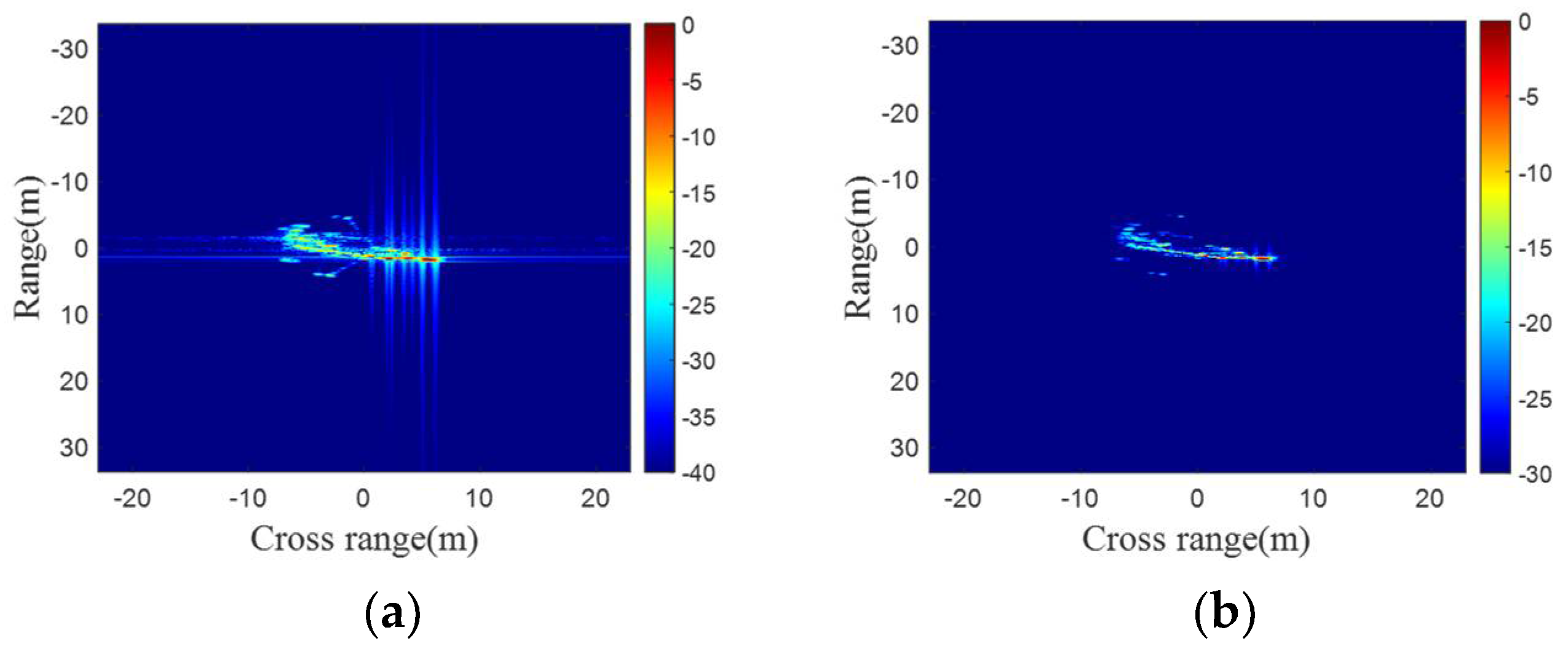
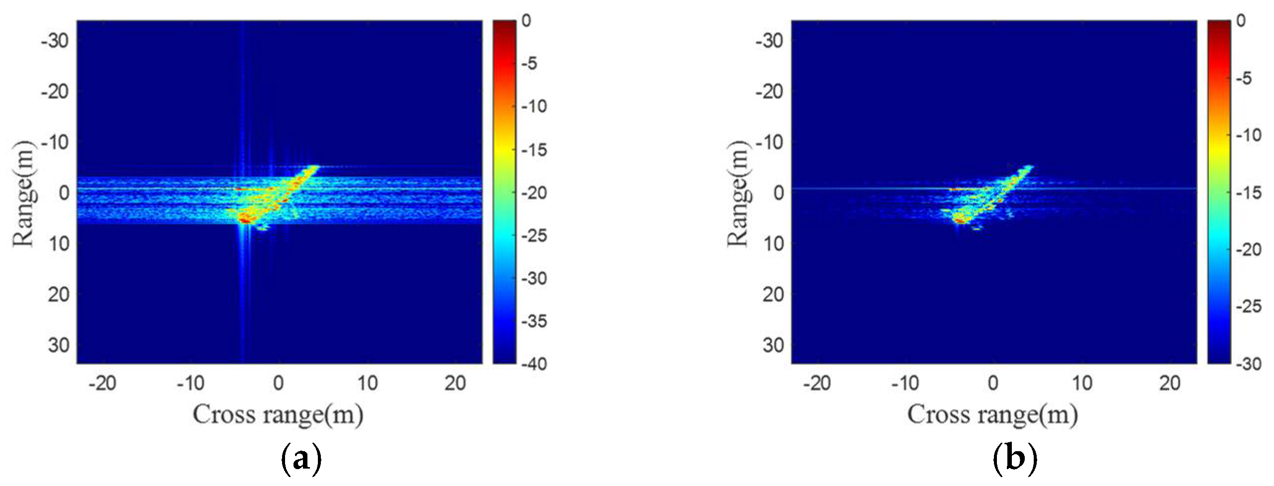
• Based on the ISAR imaging model, we deduced the cause of side-lobe noise generation in imaging. Specifically, when the difference of each scattering amplitude is too large, the side-lobe of the sinc function cannot be completely eliminated, resulting in the appearance of side-lobe noise in the ISAR image. The above conclusion has been verified through simulation and measured data;
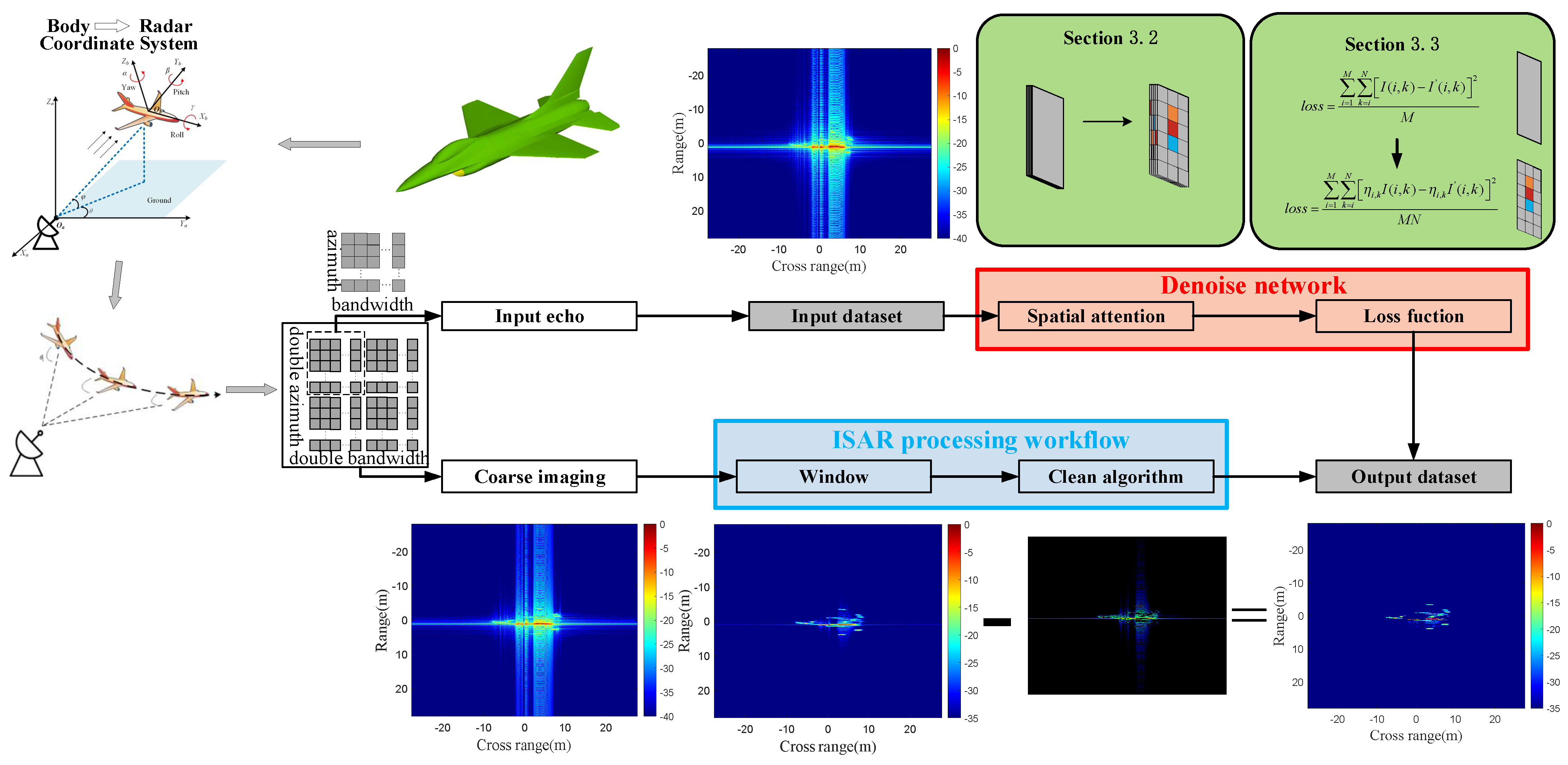
• To expedite the construction of the ISAR output dataset, we propose a fast clean algorithm. This method achieves rapid and effective side-lobe noise cancellation by implementing a high-pass filter on the range and Doppler bin;
• In the network design, we introduce a spatial attention layer and a loss function weight factor. By leveraging the sparsity of ISAR images, the noise reduction effect is enhanced, leading to a 2 dB improvement in the PSNR effect when comparing the image before and after optimization.

The organization of this paper is structured as follows. Section 2 describes the causes of side-lobe noise generation and verifies the conclusions through simulation and measured data. The fast clean algorithm, used for ISAR side-lobe denoising, is introduced in Section 3. In addition, Section 3 elaborates on the spatial attention layer and weight loss function to achieve improvement in ISAR noise reduction by reallocating the weights to the space. Section 4 focuses on the method of constructing the dataset in this paper, providing the imaging methods for different output datasets. Section 5 presents the experimental results. In this section, comparison experiments and ablation experiments are conducted to analyze the robustness of the algorithm. Section 6 provides critical summary opinions.

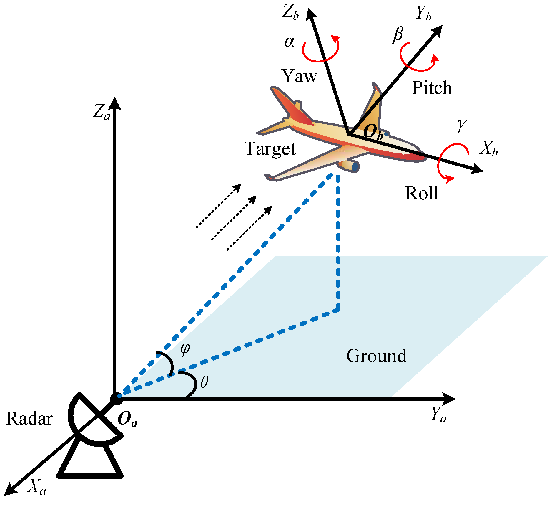
2. Problem Analysis and Sources of Ideas

2.1. Problem Analysis

The linear frequency-modulated (LFM) transmitted signal is utilized to illustrate the reasons of ISAR side-lobe noise in this paper [18,19,20]. The transmitted signal with the bandwidth $B$ and the pulse-width $T_0$ can be expressed as

$$S_0(t)=rect(\frac{t}{T_0})\exp \left(j2\pi (f_{c}t+\frac{K_r{t}^2}{2})\right)$$

(1)

where $t$ is the fast time,

$$\mathrm{rect}(\frac{t}{T_0})=\left\{\begin{array}{c}1,\left|t\right|\le \frac{T_0}{2}\\ 0,\left|t\right|>\frac{T_0}{2}\end{array}\right.$$

is a rectangular function, $f_c$ is the carrier frequency, and $K_r=B/T_0$ is the chirp rate.

For the sake of simplicity, the range migration walk [21,22] and the additive noise term are not considered in this section. Therefore, the received signal with fast time $t$ and slow time $t_m$ can be expressed as

$$S_r(t,t_m)={\sigma }_i\mathrm{rect}\left(\frac{t-2R_i(t_m)/c}{T_0}\right)\exp \left[j2\pi \left(f_c(t-\frac{2R_i(t_m)}{c})+\frac{K_r{(t-2R_i(t_m)/c)}^2}{2}\right)\right]$$

(2)

where $R_i(t_m)$ is the slant range between the radar and the generic i-th scatter $P_i(x_i,y_i)$, ${\sigma }_i$ denotes the radar cross section (RCS) coefficient of the scatter $P_i$, and $c=3\times {10}^8\mathrm{m}/\mathrm{s}$ is the speed of light.

The reference signal is

$$S_{ref}(t,t_m)=\mathrm{rect}\left(\frac{t-2R_{ref}(t_m)/c}{T_0}\right)\exp \left[j2\pi \left(f_c(t-\frac{2R_{ref}(t_m)}{c})+\frac{K_r{(t-2R_{ref}(t_m)/c)}^2}{2}\right)\right]$$

(3)

where $R_{ref}$ denotes the reference range, which is generally the distance between the target center and the radar measured by range tracking pulses.

Then, the intermediate frequency (IF) signal can be obtained via conjugate multiplication of (2) and (3).

$$S_{IF}(t,t_m)={\displaystyle \sum _i{\sigma }_i\mathrm{rect}\left[\frac{t-2R_{ref}/c}{T_p}\right]}\exp \left(-j\frac{4\pi f_c}{c}{R}_{\Delta }(t,t_m)\right)\exp \left(-j\frac{4\pi K_r}{c}{R}_{\Delta }(t,t_m)\left(t-\frac{2R_{ref}}{c}\right)\right)\exp \left(j\frac{4\pi K_r}{c^2}{R}_{{ }_{\Delta }}^2(t,t_m)\right)$$

(4)

where $R_{\Delta }(t,t_m)=R_i(t_m)-R_{ref}(t_m)$ is the range difference.

After high-speed pre-processing [23,24], range alignment [25,26], phase adjustment [27,28], and the fast Fourier transform (FFT) on the received signal in the fast time direction and the slow time direction, the received ISAR signal can be expressed as

$$S_{ISAR}(r,y)={\displaystyle \sum _i{A}_i\sin \mathrm{c}(F_x)\sin \mathrm{c}(F_y)}$$

(5)

where $F_x=\frac{\pi }{{\rho }_r}\left(r-\left(x_i+{\epsilon }_{xn}\right)\right)$ and $F_y=\frac{\pi }{{\rho }_a}\left(y-\left(y_i+{\epsilon }_{yn}\right)\right)$.$A_i={\sigma }_i{T}_p{T}_a$ is the amplitude of the scattering center located at points $(x_i,y_i)$, $T_a$ is the CPI, $\sin \mathrm{c}(u)=\sin (u)/u$ is the sinc function, $r$ is the range position, ${\rho }_r=c/(2B)$ is the range resolution, ${\epsilon }_{xn}$ is the range shift of the scatter after range alignment caused by range tracking error, $y$ is the azimuth position, ${\rho }_a=c/(2f_c{T}_{{ }_a}\sin {\theta }_n)$ is azimuth resolution, and ${\epsilon }_{yn}$ is the azimuth shift of the scatter after phase adjustment caused by the range tracking error.

Finally, after taking the modulus, normalization, and logarithm, the final ISAR imaging results can be expressed as

$$S_{final}(r,y)=10{\log }_{10}\frac{{\displaystyle \sum _i{A}_i\left|\sin \mathrm{c}\left(F_x\right)\sin \mathrm{c}\left(F_y\right)\right|}}{\max (\left|S_{ISAR}(r,y)\right|)}$$

(6)

And the ISAR image of the i-th scatter center point is

$$S_{imi}(r,y)=10{\log }_{10}\left(A_{si}\left|\sin \mathrm{c}\left(F_x\right)\sin \mathrm{c}\left(F_y\right)\right|\right)$$

(7)

where $A_{si}=\frac{A_i}{\max (\left|S_{ISAR}(r,y)\right|)}$.

In simple ISAR scenarios, such as some angles of satellite and non-stealth aircraft, an impulse function can be transformed from the sinc function by a suitable truncation threshold. However, for the stealth targets and some special angles of the satellite and non-stealth target, it is difficult to achieve the transformation from ‘sinc’ to ‘impulse’.

For simplicity we will focus on the ISAR image scenarios of the two scatters, and without loss of generality we assume the two scatters are located at (0,0), $(x_n,y_n)$, and ${\epsilon }_{xn}={\epsilon }_{yn}=0$. Then, (7) can be rewritten as follows:

$$S_{im1}(r,y)=10{\log }_{10}\left(A_{s1}\left|\sin \mathrm{c}(\frac{\pi }{{\rho }_r}r\left)\sin \mathrm{c}\right(\frac{\pi }{{\rho }_a}y)\right|\right)$$

(8)

$$S_{im2}(r_i,r_m)=10{\log }_{10}\left(A_{s2}\left|\sin \mathrm{c}\left(\frac{\pi (r-x_n)}{{\rho }_r}\right)\sin \mathrm{c}\left(\frac{\pi \left(y-y_n\right)}{{\rho }_a}\right)\right|\right)$$

(9)

Then, while the p-th side-lobe of the first scatter points appears in $(r_i,r_m)$, where $\sin (\frac{\pi r_i}{{\rho }_r})=1,r_m=0$; the amplitude of the ISAR influence induced by the first point yields

$$S_{im1}(r_i,0)=10{\log }_{10}(A_{s1}\frac{{\rho }_r}{\pi r_i})$$

(10)

$$S_{im1}(l\frac{c}{2B},0)>\max (S_{im2}(r_i,r_m))=10{\log }_{10}(A_{s2})$$

(11)

When it satisfies (11), a new challenge arises in ISAR image processing; that is, how to attenuate side-lobe noise while retaining weak scattering centers? Despite the third side-lobe experiencing an attenuation of approximately 20 dB, the intensity of some weak scatter points is lower than those of the side-lobe, due to the emergence of structural stealth technology and the presence of creeping waves and detour waves. Furthermore, motion compensation, the primary focus of ISAR imaging research, does not assist in resolving this issue, which persists even with ideal echoes.

Without loss of generality, two toy simulation experiments are designed in this paper to validate the effectiveness and superiority of the above-mentioned conclusion. For the convenience of discussion, the same ISAR system is applied in these two experiments, and the corresponding parameters are listed in

Table 1. The main parameters for the ISAR system.

Parameters	Value
Pulse repletion frequency (PRF)	40 Hz
Bandwidth	2 GHz
Pulse width	25 μs
Carrier frequency	10 GHz
Sampling frequency	32 MHz
Observing time	10 s

.

(1) Simulation based on the scattering center model.

A toy control experiment is designed to illustrate that the amplitude gap between the different scatter points is the core aspect of the problem. According to the GTD model [29,30,31,32], the electromagnetic scattering echo can be expressed as

$$s(f_m,{\theta }_n)=A{(j\frac{f_m}{f_c})}^{\alpha }\exp (-j\frac{2\pi f_m}{c}(x\cos {\theta }_n+y\sin {\theta }_n))$$

(12)

where $f_m=f_0+m\Delta f,m=0,1\dots M$, $f_0$ represents the initial frequency, $\Delta f$ denotes the frequency step, m is the frequency index, ${\theta }_n={\theta }_0+n\Delta \theta$, ${\theta }_0$ is the initial radar line-of-sight angle, $\Delta \theta$ denotes the relatively small radar rotation angle, and n is the angle index. In this paper, the target rotates around the reference center at a constant speed. Specifically, ${\theta }_n={\theta }_0+nw{t}_m$, $w=\frac{0.4\pi }{180}\mathrm{rad}/s$.

The above scattering echo satisfies the assumption of the far-field plane wave, thus the target ISAR image can be obtained by applying the 2D Fourier transformation on the target echo according to the range-Doppler (RD) algorithm. The parameters of the scattering centers are listed in

Table 2. The parameters of the 1st experiment.

Scattering Centers	${\mathit{x}}_{\mathit{i}}/\mathbf{m}$	${\mathit{y}}_{\mathit{i}}/\mathbf{m}$	${\mathit{\alpha }}_{\mathit{i}}$	${\mathit{A}}_{\mathit{i}}$
Scattering center 1	0.1	0.1	0	1
Scattering center 2	5	5	1	5
Scattering center 3	10	−5	0.5	8
Scattering center 4	−5	10	−1	10
Scattering center 5	−10	−10	−0.5	20

and

Table 3. The parameters of the 2nd experiment.

Scattering Centers	${\mathit{x}}_{\mathit{i}}/\mathbf{m}$	${\mathit{y}}_{\mathit{i}}/\mathbf{m}$	${\mathit{\alpha }}_{\mathit{i}}$	${\mathit{A}}_{\mathit{i}}$
Scattering center 1	0.1	0.1	0	1
Scattering center 2	5	5	1	5
Scattering center 3	10	−5	0.5	50
Scattering center 4	−5	10	−1	100
Scattering center 5	−10	−10	−0.5	200

.

The above two experiments only change the scattering amplitude, and the imaging results using the different truncation threshold ${\epsilon }_I$ are shown in Figure 1 and Figure 2.

Figure 1 demonstrates the imaging results obtained under various ${\epsilon }_I$ with similar scattering point amplitudes. The ISAR image generated by the point echo model contains stripe structures, which will lead to strong scattering points, as observed in Figure 1. Following normalization, the amplitudes of each scattering point are expressed as relative magnitudes. In the case of a single scattering center, the side-lobe noise is lower than the main-lobe signal. However, comparing different scattering centers, the side-lobe amplitude of the strong scattering center remains higher than the main-lobe signal of the weak scattering centers. Consequently, to preserve the weak scattering centers, the ISAR image consisted of a portion of side-lobe signals, resulting in the stripe appearance of the point scattering center.

The determination of the truncation threshold becomes unattainable when there is a significant widening of the amplitude gap, as shown in Figure 2. In Figure 2b, the side-lobe of scattering center 5 remains at an amplitude of −16 dB after attenuation, while the main lobe of scattering center 1 only reaches −15 dB. In this scenario, both the RD-based imaging algorithm and its corresponding improved methods fail to suppress the side-lobe noise and achieve imaging of the weak scattering point simultaneously. Furthermore, owing to the substantial difference in amplitude, the weak scattering point contributes only 0.01% of the total image energy. In this situation, the compressed sensing-based methods fail to demonstrate the weak scattering points, leading to incomplete imaging information, for the reason that the iteration termination condition is determined by the energy recovery ratio.

(2) Simulation based on the electromagnetic models.

Another experiment involves using an electromagnetic model to capture echoes. In this paper, we are aiming to address the issue of information loss during side-lobe noise reduction. The accuracy of the target computer-aided design (CAD) model is not a critical factor, so a model from a public website [33] is used for simulation experiments. We utilize the same ISAR imaging system to simulate two aircraft, one with a non-stealthy structure and another with a stealthy structure. The electromagnetic simulation models are depicted in Figure 3.

Electromagnetic calculations are performed on the target simulation models, and target echoes are generated by using trajectory modeling and coordinate conversion. Subsequently, the RD algorithm is applied for target ISAR imaging. Additionally, the imaging effect is enhanced by adding windows and zero padding operations. The purpose is to illustrate that the special structure of the aircraft will bring out a large difference in the amplitude between the strong and weak scattering points. The above scattering intensity difference is due to lead to excessive side-lobe noise, which will deteriorate the ISAR quality in a large degree. The ISAR images of the non-stealth aircraft, the special angles of the non-stealth aircraft, and the ISAR imaging results of the stealth aircraft are shown in Figure 4 and Figure 5 and Figure 6 and Figure 7, respectively.

Figure 4 and Figure 5 depict the imaging outcomes for a non-stealth aircraft; here, $\theta$ is the azimuth angle and $\phi$ is elevation angle. Generally, for most observing angles, the truncation threshold can achieve retention of scattering point information and eliminates side-lobe noise in ISAR images. However, while decreasing the threshold will inevitably lead to the loss of information on weak scattering points, which can be depicted in Figure 5, those lost weak scattering points, distributed in the wings and tails of the aircraft, play a crucial role in enhancing the imaging quality and target recognition accuracy.

However, for some special angles ($\theta$ is from ${36}^{\circ }$ to ${41}^{\circ }$), such as in Figure 6, the radar observing angle appears significantly higher in magnitude compared with other positions of the strong scattering points. Consequently, the main power of the final processing results lies in the strong scattering centers and side-lobe noise, rather than the weak scattering points. The above-described phenomenon is quite common in stealth aircraft imaging tasks. Figure 7 presents the ISAR imaging results of a typical stealth aircraft. Considering the effect of stealthy structure, the overall scattering amplitude of the aircraft is relatively low, and the strong scattering region only appears at the observing angle. As shown in Figure 7, compared with the strong scattering region, the relative magnitude of the remaining portion of the aircraft is below −20 dB, which is similar to the simulation experiment results of the first point scattering center model. The above analysis implies an identical conclusion that conventional imaging methods cannot remove such noise. Additionally, in the complex imaging results, strong scattering points become strong scattering areas, which degrades the imaging quality of the clean algorithm. It should be noted that the above-mentioned problem also exists in some real raw radar processing data, which can be shown in Figure 8.

Figure 8 depicts the space shuttle Atlantis ISAR image at various observed angles, which are obtained using the German TIRA synthetic aperture radar. The aircraft’s features at different angles are similar, but the presence of side-lobe noise significantly alters the features, which will deteriorate the target recognition accuracy.

By taking insight from the above simulation results and real raw data processing results, it can be summarized that the reason for this problem is the sinc function and the target structure, which is a corollary of the Fourier transform-based imaging method. The core ideas of the present imaging algorithms mainly focus on the target motion compensation while they do not solve the side-lobe noise problem in an effective way. In reality, the side-lobe noise of ISAR images is similar to the rain noise from the essential aspect. Motivated by the aforementioned analysis, a denoise network is proposed for removing side-lobe noise in this paper, which effectively alleviates the target recognition problem caused by the poor quality of ISAR imaging. Furthermore, considering the sparsity of ISAR images compared with optical photographs, we introduce a spatial attention block into the traditional network and optimize the loss function. A complete source of ideas is shown in the following section.

2.2. Sources of Ideas

Image denoising aims to recover the high-quality image X from the degraded measurement $\mathit{Y}$ [13,21,34,35,36]. The degradation process is generally defined as

$$\mathit{Y}=\mathit{A}\mathit{X}+\mathit{n}$$

(13)

where $\mathit{A}$ is the degradation matrix, and $\mathit{n}$ represents the additive noise. The fundamental objective of rain and fog noise removal in optics and side-lobe noise decreasing in radar imaging is the restoration of image X. Here, we discuss the similarities and differences between these two types of noise reduction problems. Examples of rain denoise and side-lobe denoise are shown in Figure 9.

From Figure 9, it is evident that rain noise and ISAR side-lobe noise share similar characteristics, both displaying the straight lines traversing the image. However, there are also notable differences between them.

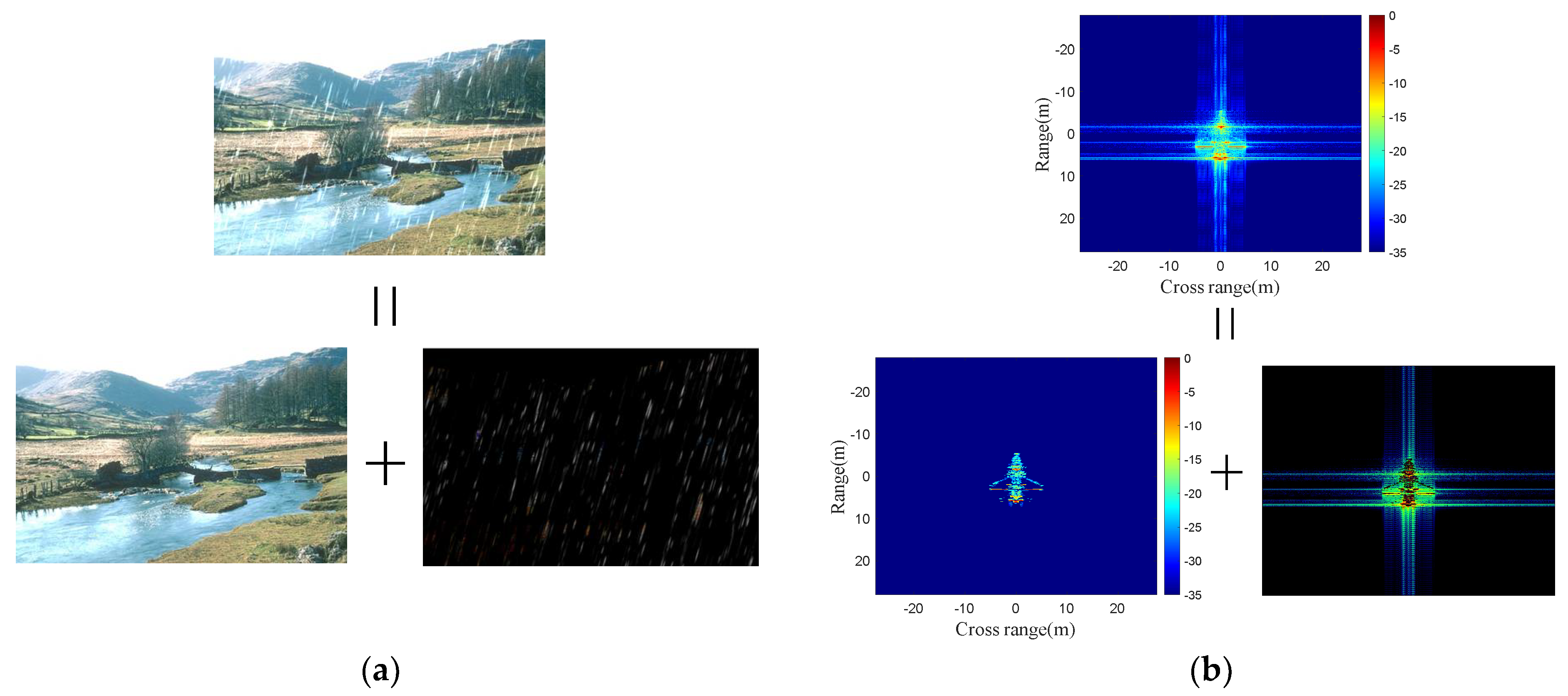
• Different causes. In optical imaging, rain noise occurs because light, with its long wavelength and weak bypass ability, cannot pass through raindrops, resulting in rain noise in the image. In radar images, as discussed in Section 2, the presence of the sinc function in the imaging result causes side-lobe noise higher than the weaker scattering points;
• Noise behavior. The performance of the noise differs as well. Rain noise in the image ‘covers’ the target image, while in radar images, the side-lobe noise and the target image are superimposed;
• Spatial distribution. The two types of noise manifest in different areas. Rain noise is distributed throughout the image, with a relatively fixed distribution position. On the other hand, side-lobe noise only appears near strong scattering points, and its position changes with the position of the strong scattering point.

In this paper, two improvements are made to the traditional noise reduction network.

• A novel spatial attention layer construction is applied in the network structure by our paper;
• An adaptive magnitude factor is designed to describe the loss function more accurately.

Figure 10 depicts the flow chart of this entire paper. The main contribution of this paper can be summarized as the following two parts: dataset construction and network training. In dataset construction, the core idea is to propose a new ISAR processing principle, which can optimize the clean algorithm to construct the output dataset. Regarding network training, this paper introduces the spatial attention block and optimizes the loss function based on the above analysis, making the traditional noise reduction network more suitable for ISAR parallax noise reduction. The above work is described in Section 3.

3. The Proposed Methods

3.1. The Fast Clean Technique

How to construct clean ISAR images is the first problem to be addressed in this paper. The existing clean algorithm based on the PSF faces challenges such as difficult iteration termination condition setting and large computational volume for point-by-point clean operation. To address the above-mentioned problems, we adopt a fast clean algorithm in this section (Algorithm 1). Compared with the classical clean algorithm, the fast algorithm performs bin-by-bin (range bin and Doppler bin) clean operation by setting a threshold along the range bin, and using the mean value of each range bin as the threshold for high-pass filtering processing. After completing processing in the range dimension, the same processing is performed in the azimuth dimension.

Algorithm 1: The fast clean algorithm

Input: A signal matrix with side-lobe noise $S\in R^{H\times W}$ High-pass filtering threshold adjustment factor ${\alpha }_1,{\alpha }_2$ The function of the high-pass filter $\varpi$ Output: A clean signal matrix $S^{\prime }\in R^{H\times W}$

for i = 1 to H Calculate the high-pass filter threshold $\chi ={\alpha }_1\times \mathrm{sum}(S(i,:))$ High-pass filtering for each range bin $S^{\prime }(i,:)=\varpi (S(i,:))$ for j = 1 to W $\chi ={\alpha }_2\times \mathrm{sum}(S(:,j))$ $S^{\prime }(:,j)=\varpi (S(:,j))$

Compared with the traditional method, the fast clean algorithm reduces the number of iterations and only requires $H\times W$ sub iterations to complete the processing of the whole image. In addition, in each iteration, the fast clean algorithm only needs to perform the size comparison operation, which avoids the matching process of the traditional method using PSF and reduces the computational complexity significantly.

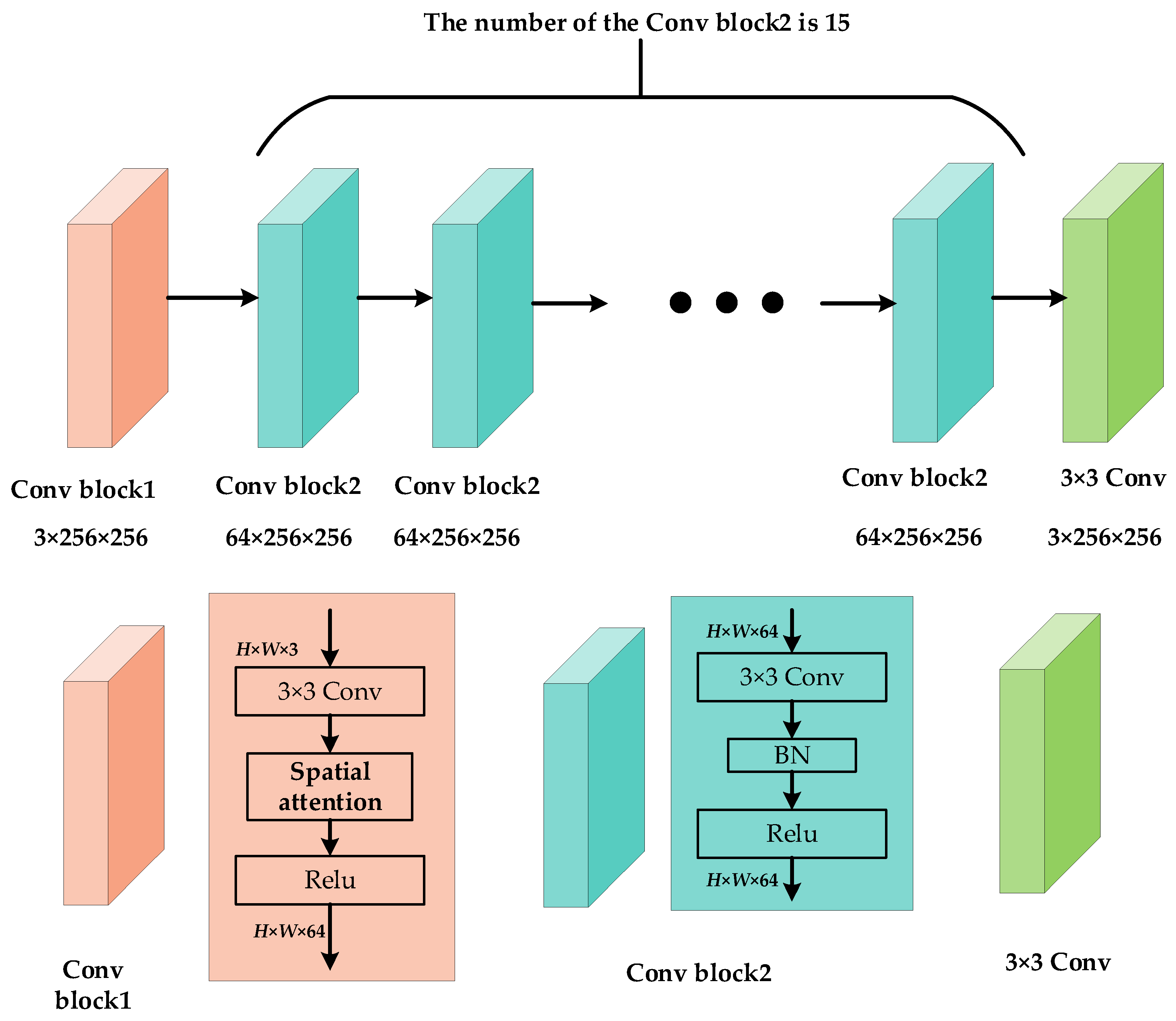
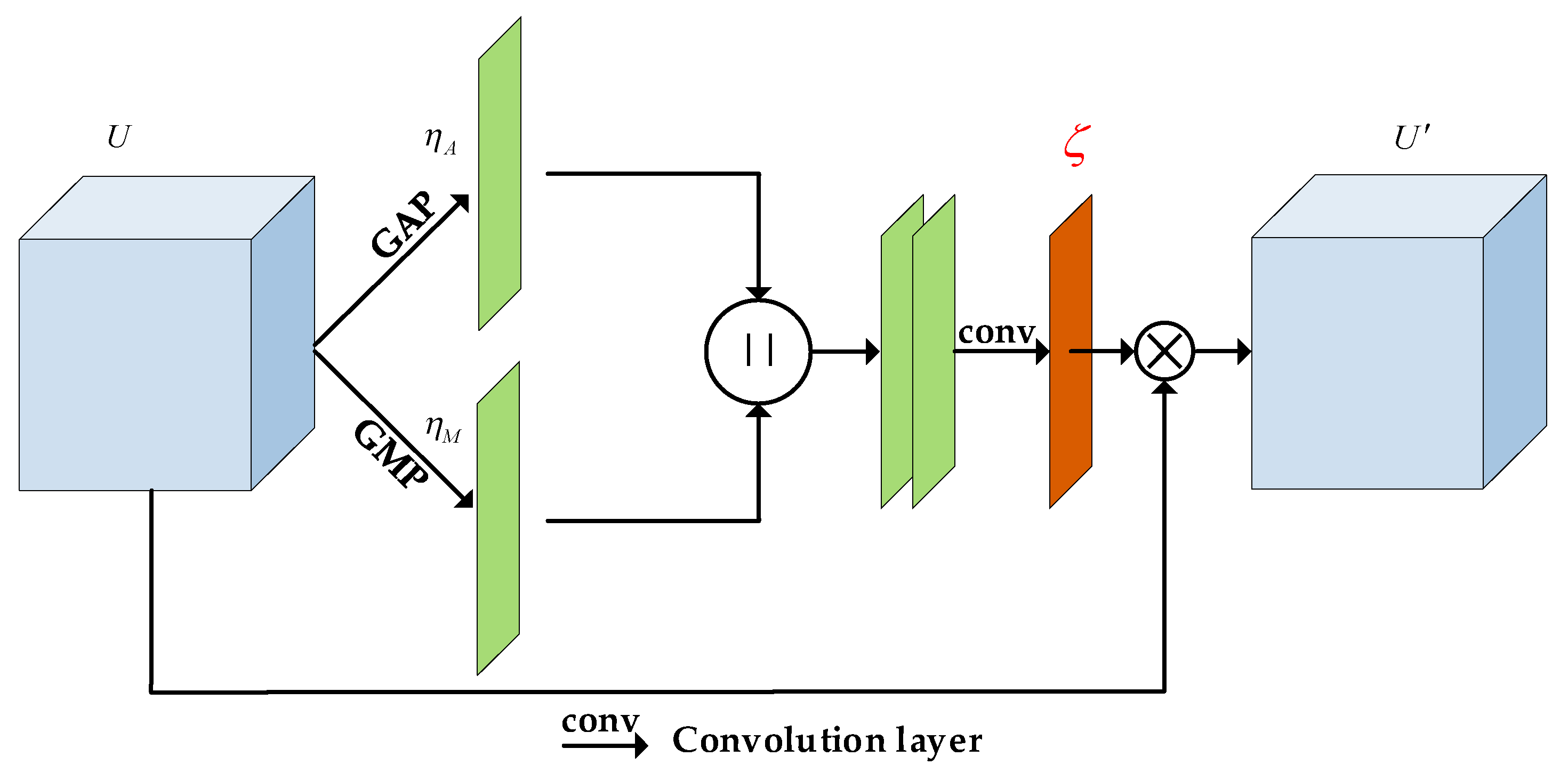
3.2. The Spatial Attention Block

Eliminating the side-lobe noise in the ISAR image is a challenging task. The information within ISAR images comprises three main components: background, side-lobe noise, and target features. In an ISAR image, the majority of the region contains background information. Excessive background information and unknown target features necessitate a greater focus on the spatial dimension. Moreover, different from the optical rain noise pictures, the distribution of ISAR parallax noise is more concentrated, and the rapid focusing of the core region via the spatial attention module is beneficial for improving convergence speed. Therefore, to enhance the performance of ISAR image denoising, we introduce the spatial attention block to capture the target features. The spatial attention block architecture is shown in Figure 11 and detailed introduction of the spatial attention block is shown as follows.

In the spatial attention block, the collection of spatial weight $\zeta \in R^{H\times W\times C}$ is our goal, which is applied to rescale spatial feature maps to generate recalibrated features. The spatial descriptor ${\eta }_A,{\eta }_M$ can be obtained by squeezing global information using the GAP layer and the GMP layer. Then, it is followed by a concatenation layer to concatenate the two spatial descriptors. In the end, a convolution layer, whose kernel size is 5 × 5, is used to summarize the spatial descriptor and obtain the spatial weight $\zeta$. The above process can be formulated as

$${\eta }_A=GAP(U)$$

(14)

$${\eta }_M=GMP(U)$$

(15)

$$\zeta =Sigmoid(Con{v}^{5\times 5}(Concatenate({\eta }_A,{\eta }_M)))$$

(16)

where $Con{v}^{n\times n}$ denotes the convolution layer in which the kernel size is n × n; $U$ is the feature map of the last layer input.

The final output of the spatial attention module is obtained with

$$U^{\prime }=U\otimes \zeta$$

(17)

where $U^{\prime }$ is the output of the spatial attention module, and $\otimes$ is the element multiplication.

The spatial attention block focuses on spatial weight redistribution. Unlike the channel attention, the spatial attention focuses on ‘where’ an informative part is, which is complementary to the channel attention. The spatial attention block, as a simple module, can bring about iterative stability and improved noise reduction with a constant number of parameters. The later experiments verify these conclusions.

3.3. Loss Function

In addition, this paper optimizes the loss function. Conventional noise reduction networks typically use mean square error as the loss function to assess the disparity between the predicted value and the true value. Mean square error is suitable for evaluating optical images, as illustrated in Figure 9a, where the noise is distributed across the entire image and there is no variation in the weights among the pixel points. However, for radar images, as depicted in Figure 9b, the noise is concentrated in the center and the significance of the pixels varies significantly. Therefore, this paper proposes the mean square loss function with a magnitude factor to address this issue. The function expression is as follows:

$$loss=\frac{{\displaystyle \sum _{k=1}^N{\displaystyle \sum _{i=1}^M{\kappa }_{i,k}{(I(i,k)-K(i,k))}^2}}}{M}$$

(18)

where $I(i,k)$ is the value of the output image of the network in row i column k, $K(i,k)$ is the value of the target output image in row i column k.$I(i,k)$ and $K(i,k)$ are $M\times N\times 3$. ${\kappa }_{i,k}$ is the introduced magnitude factor, which is calculated as follows:

$${\kappa }_{i,k}=\frac{e^{K(i,k)}}{{\displaystyle \sum _{k=1}^N{e}^{K(i,k)}}}$$

(19)

The equation can be thought of in images as assigning weights based on image depth, whereas for radar imaging matrices, (19) implies operating a softmax assignment of weights to each range bin. The traditional loss function has a descent rate for each cell of $-2(I(i,k)-K(i,k))$, while the optimized descent rate is $-2{\kappa }_{i,k}(I(i,k)-K(i,k))$. For scattering points, the descent rate is higher than the traditional loss function. For the background region, the accuracy of the values is not important, thus the difference in the descent rate can be ignored.

4. The Dataset Construction

To learn various parameters in the denoise network, it is crucial to construct an appropriate training dataset. A simple and convenient method for constructing a dataset is to use the scattering center model. This approach can generate a large number of ISAR images by varying the scattering center numbers, scattering amplitudes, and scattering center locations. In this paper, we use this method to generate a pre-training set to initially train the network. However, the ISAR images generated by this method cannot accurately depict the coupling characteristics between different scattering centers and do not simulate the side-lobe noise caused by the structure. Therefore, we also construct a post-training dataset based on the electromagnetic simulation model to enhance the network’s noise reduction performance. The specific process of our dataset construction method is demonstrated as follows.

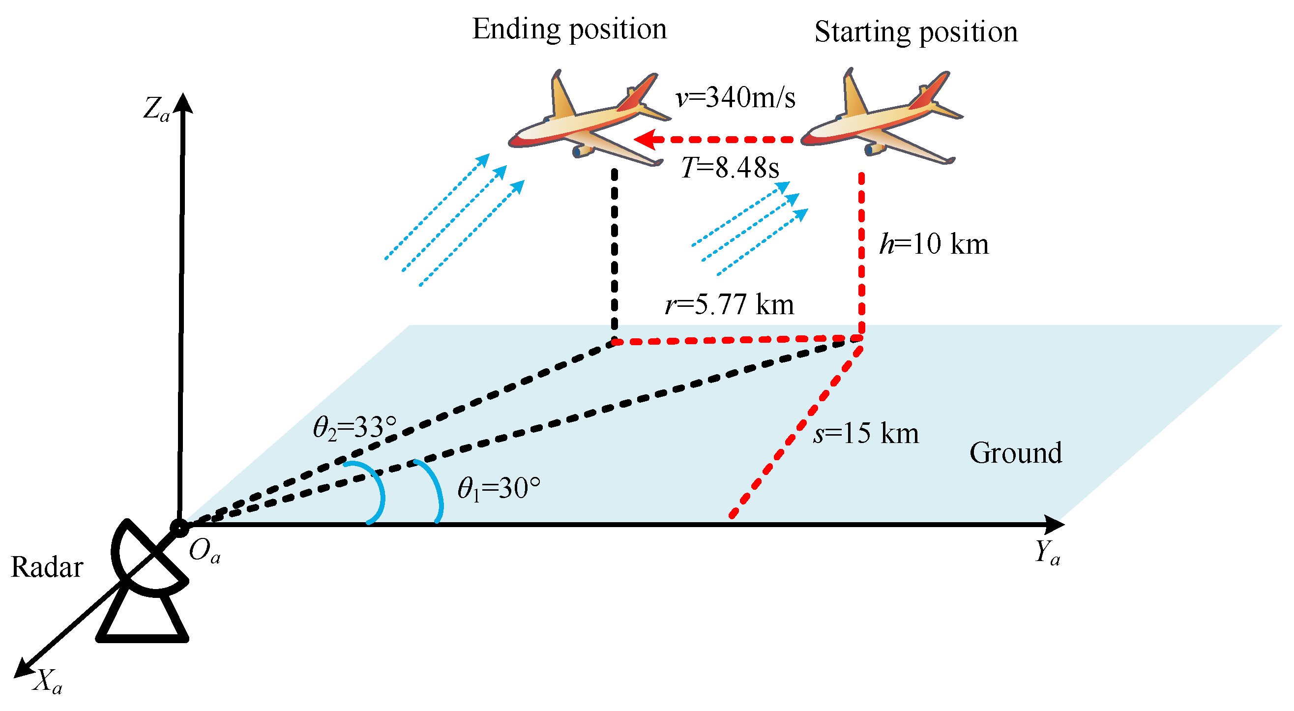
4.1. The Dataset Based on the GTD Model

The dataset construction, based on the GTD model, can be divided into the following four steps:

Step 1 Calculating the imaging interval.

$$X={\rho }_{r}M=\frac{c}{2B}M=\frac{c}{2M\Delta f}M=\frac{c}{2\Delta f}$$

(20)

$$Y={\rho }_{a}N=\frac{c}{(2f_c{T}_{{ }_a}\sin {\theta }_n)}N$$

(21)

where X represents the maximum span in the distance direction, and M = 800 is the total number of range positions, corresponding to the number of frequency points in the GTD model. Similarly, $Y$ denotes the maximum span in the azimuth direction, and N = 200 is the total number of azimuth positions, corresponding to the number of azimuth points in the GTD model.

Based on (13), (14), and the radar parameter settings in Section 2, the imaging interval is calculated as $\Delta f=2.5\mathrm{MHz}$, ${\rho }_r=0.075$, X = 60 m, and Y = 40 m. To enhance the generality of the constructed dataset, this paper generates a point scattering center model dataset by randomizing the position, number, and magnitude, instead of constructing a scattering center model for a specific type of target;

Step 2 Target electromagnetic echo generation.

The number of target scattering points is randomly generated by selecting a random integer within the range of 50~100 as the number of scattering centers. Twenty percent of the points were designated as strong scattering points, while the remaining were categorized as weak scattering points. The amplitude of the strong scattering points was randomized to be a normally distributed random number within 100~1000, and the weak scattering points were assigned a normally distributed random number within the range of 1~50. The GTD model parameter settings are completed by randomly assigning position and scattering type to each scattering point. Finally, the target echo data can be generated according to Equation (12);

Step 3 Input dataset construction.

Using the echoes obtained in Step 2, the RD algorithm is employed to construct the target input ISAR image. To introduce randomness, different truncation thresholds are selected for imaging, ensuring that the weakest scattering point remains present;

Step 4 Output dataset construction.

Under high frequency conditions, the radar target echo can be considered as the sum of each independent scattering center. In this paper, each scattering center is initially imaged independently to obtain the ISAR imaging of a single scattering center. Subsequently, the threshold is used as the termination condition to obtain the main lobe scattering matrix of each scattering center and its corresponding position. Finally, the ISAR image with the smallest scattering amplitude is replaced in the ISAR image for each position of the scattering matrix to generate the target output image. The input and output images are shown in Figure 12.

4.2. The Dataset Based on the Electromagnetic Simulation Model

In this section, we generate the output dataset utilizing the electromagnetic model of the target, as depicted in Figure 3a.

(1) The process of echo simulation.

The coordinates used in the trajectory modeling are in the radar coordinate system, while echo calculation is in the body coordinate system coordinates. Therefore, before performing echo calculation, coordinate transforms are necessary. Firstly, the definition of the coordinate system used in this paper is introduced.

1. Radar coordinate system $O_a-X_a{Y}_a{Z}_a$.

As shown in Figure 13, it takes the radar station location as the origin $O_a$. The $X_a$ axis points to the east pole, the $Z_a$ axis points to the sky, perpendicular to the ground, and the $Y_a$ axis points to the North direction, forming a right-hand coordinate system with X and Y;

2. Body coordinate system $O_b-X_b{Y}_b{Z}_b$.

The target body coordinate system is rigidly connected to the target structure, as shown in Figure 13, with its origin located at the mass center of the target. The $X_b$ axis points to the nose direction of the target within the symmetry plane, and the $Y_b$ axis is perpendicular to the $X_b$ axis and aligned with the high direction within the symmetry plane. The $Z_b$ axis forms a right-hand coordinate system with X and Y.

The coordinate transformation formula is as follows:

$$\mathit{P}\prime =R_x(\gamma )R_y(\theta )R_z(\varphi )\times {\mathit{P}}_0=\left[\begin{array}{ccc}1& 0& 0\\ 0& \cos \gamma & \sin \gamma \\ 0& -\sin \gamma & \cos \gamma \end{array}\right]\left[\begin{array}{ccc}\cos \theta & 0& -\sin \theta \\ 0& 1& 0\\ \sin \theta & 0& \cos \theta \end{array}\right]\left[\begin{array}{ccc}\cos \varphi & \sin \varphi & 0\\ -\sin \varphi & \cos \varphi & 0\\ 0& 0& 1\end{array}\right]\left[\begin{array}{c}{x}_m\\ y_m\\ z_m\end{array}\right]$$

(22)

where $\gamma$, $\theta$, and $\varphi$ correspond to the angles generated by yaw, pitch, and roll, ${\mathit{P}}_0$ represents the coordinates of the target in the radar coordinate system, and $\mathit{P}\prime$ is the coordinates of the radar in the body coordinate system.

Then, it is assumed that a radar operates in the X-band with an operating frequency of 10 GHz, a bandwidth of 1 GHz, and a transmitted signal as a linear frequency modulation signal. It is also supposed that the target rotates by $3^{\circ }$ within the imaging range, emitting 150 pulses within the range, and each pulse contains 401 range cells, constructing the target echo scene accordingly.

The flight trajectory, as shown in Figure 14, assumes the target flight height is 10 km, the route shortcut is 15 km, the flight speed is 340 m/s, the flight direction is parallel to the $Y_a$ axis, the imaging accumulation time is 8.48 s, the flight distance is 5.77 km, the azimuth angle changes from ${30}^{\circ }$ to ${33}^{\circ }$, and the pitch angle changes from ${18.33}^{\circ }$ to ${19.96}^{\circ }$.

The azimuth and pitch angles in the body coordinate system are calculated using Equation (22). The azimuth angle is set to be same in the radar coordinate system, and the pitch angle changes from ${108.33}^{\circ }$ to ${109.96}^{\circ }$. Given the number of transmitted pulses and range bins, computing the echo data includes a total of 401 frequency points and 150 position points. Finally, add the equivalent delay to each echo datum. The above descriptions are the specific dynamic radar data acquisition process.

As shown in the coordinate transformation matrix, the azimuth angle changes remain the same when the target flight direction is parallel to the $X_a$ axis or $Y_a$ axis. The slight change in pitch angle during a cycle has a negligible effect on the change in echo amplitude. To simplify the echo construction method, we select a fixed pitch observing platform to compute static data for targets from 0 to 360 azimuth angles. Slicing the data with $1^{\circ }$ intervals will generate an 801 × 401 data matrix per slice, containing 401 pulse data points and 801 range cell data points. Finally, the construction of the echo dataset is completed by varying the pitch observing platform;

(2) The process of output dataset.

The construction of the target output set involves three main steps: windowing, cleaning, and imaging.

Step 1 Windowing and cleaning.

In this step, a Hamming window is added to the echoes obtained in the previous section. After adding the Hamming window, the side-lobe noise persists, and a fast clean algorithm proposed in this paper is required to enhance the imaging quality;

Step 2 Imaging.

Finally, RD imaging is performed on the processed echoes to obtain the output dataset;

(3) The process of input dataset.

The output set is constructed using a window function that reduces the resolution. To ensure similarity in resolution between the input and output sets, the number of pulses and distance bin of the input set are adjusted to be consistent with the output set. The RD imaging method is utilized to construct the target input set. Once the input set is constructed, the input image and output image are aligned. The construction of the input set is then completed. The imaging results of the input set and output set are depicted in Figure 15.

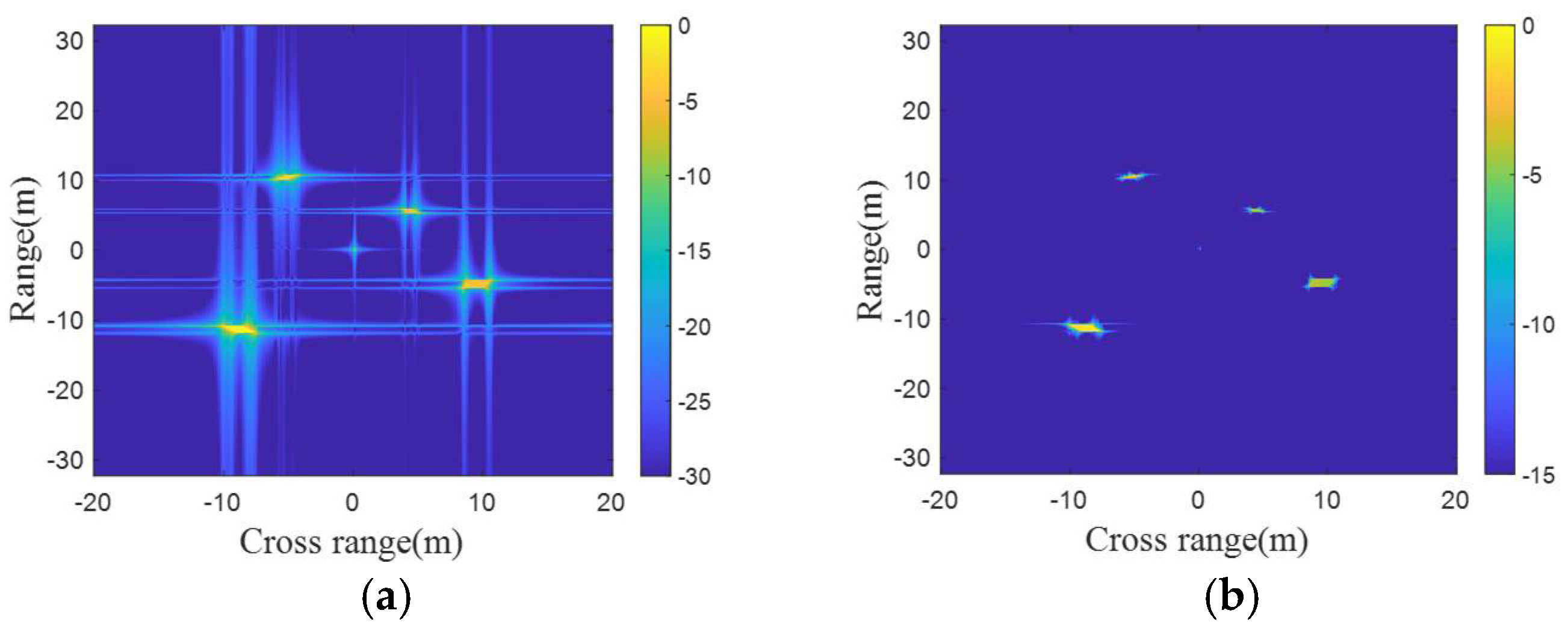
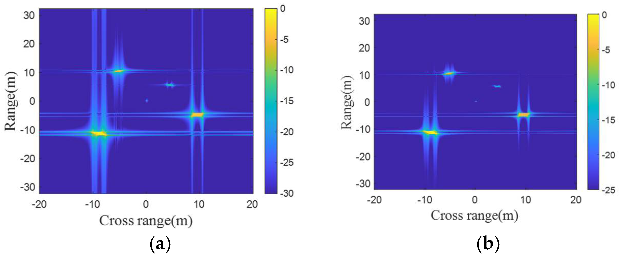
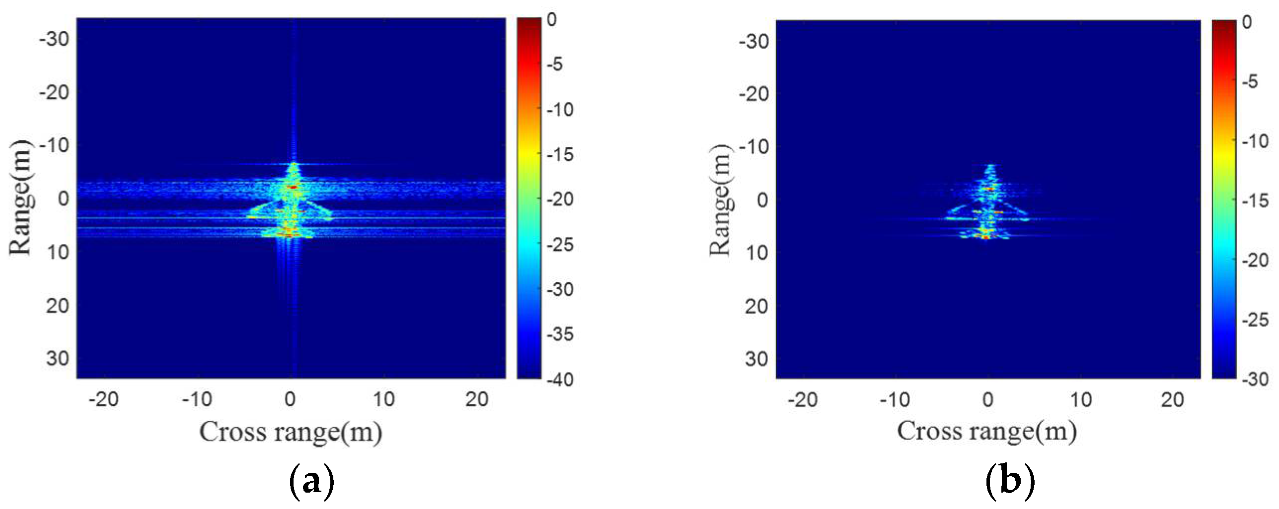
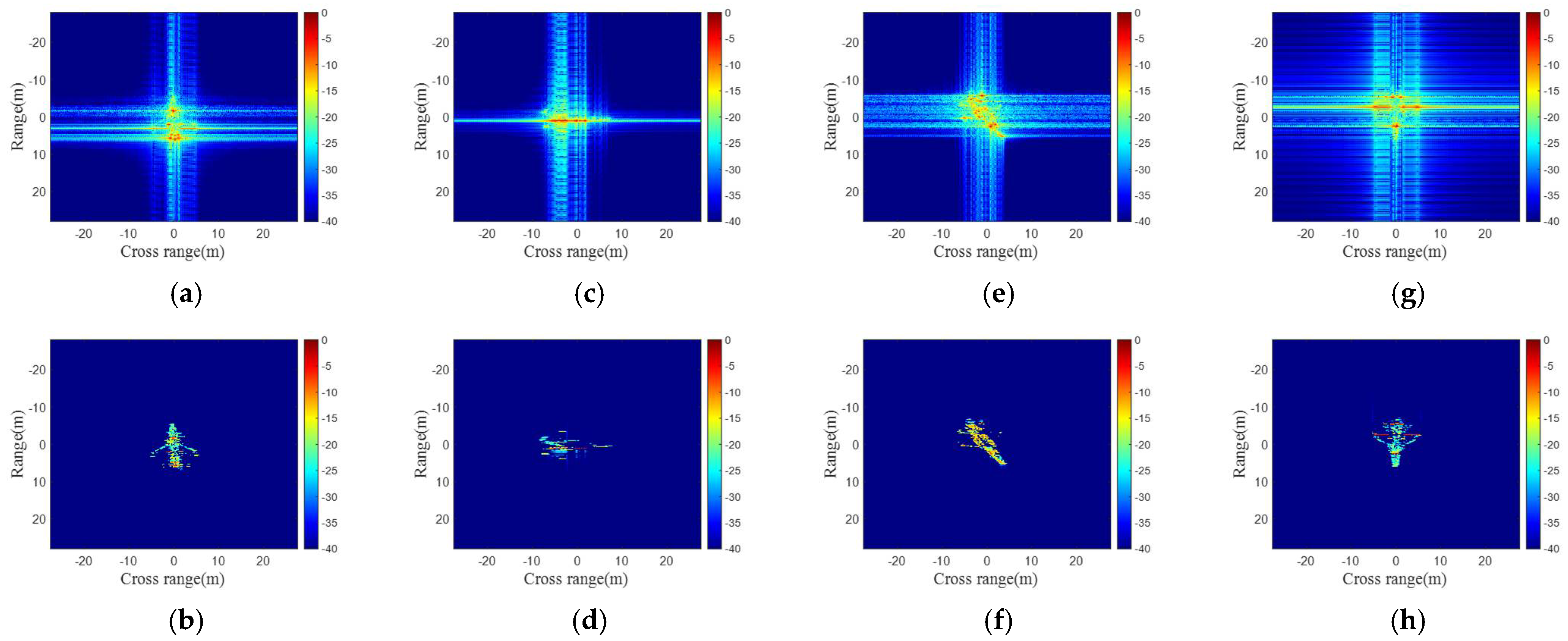
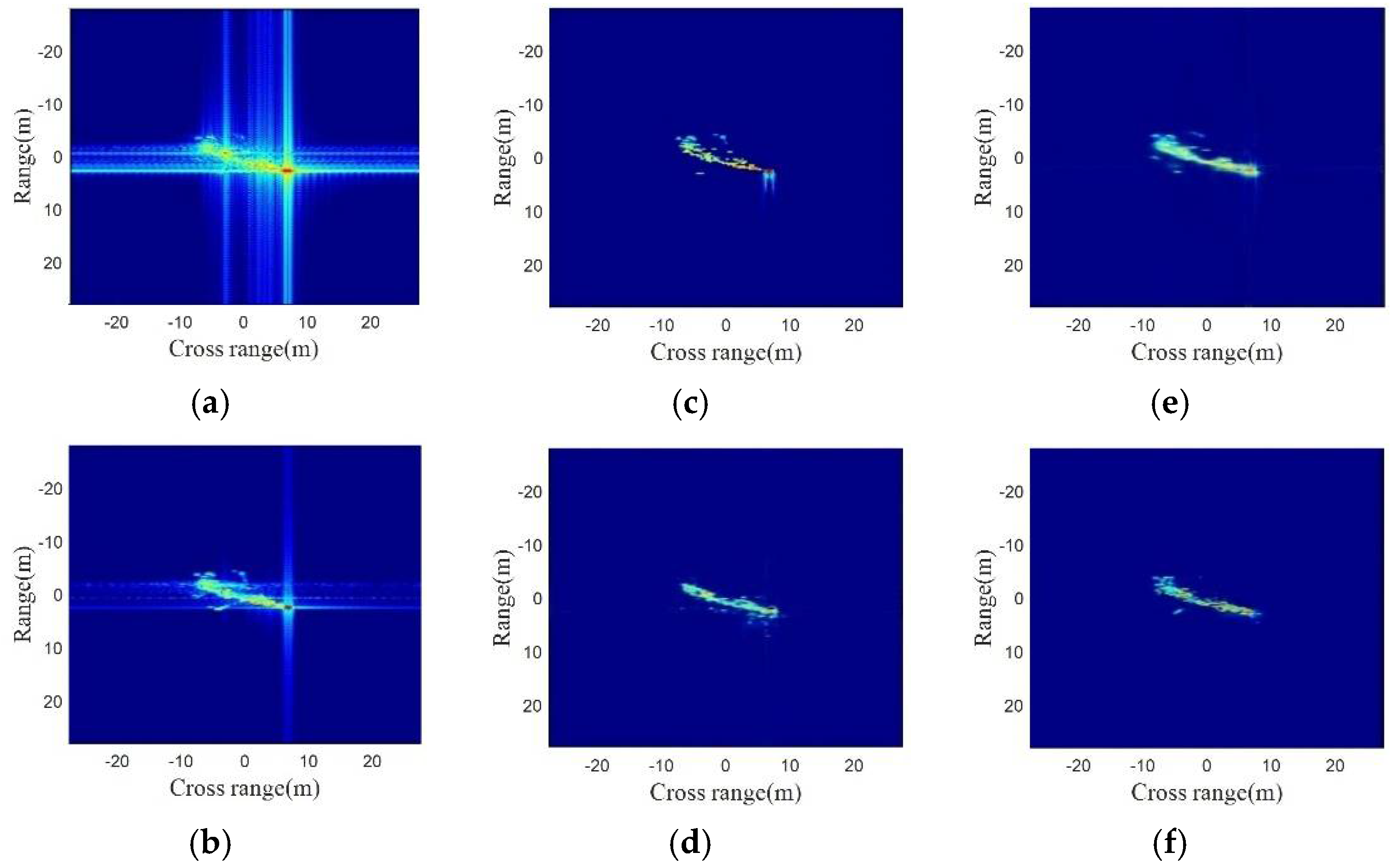
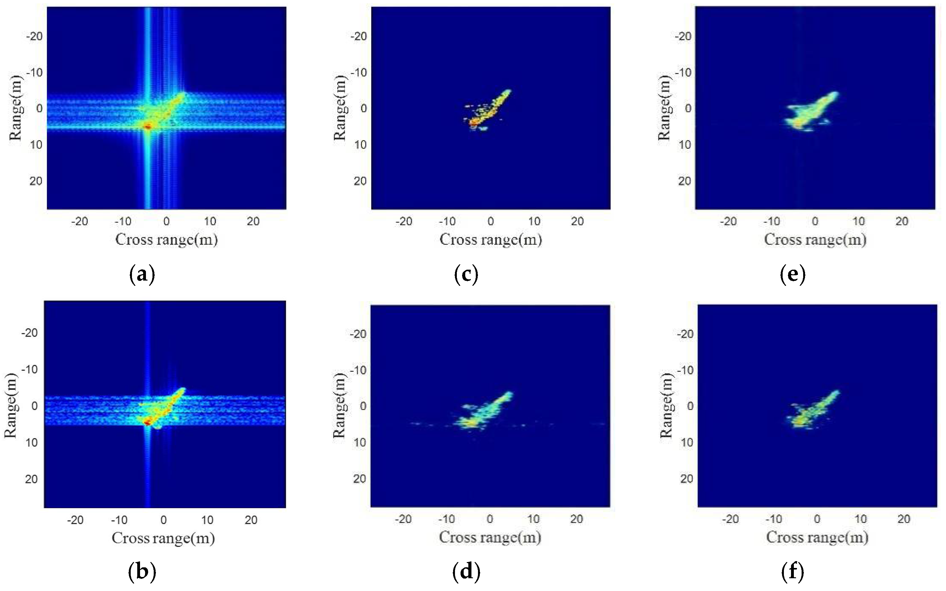
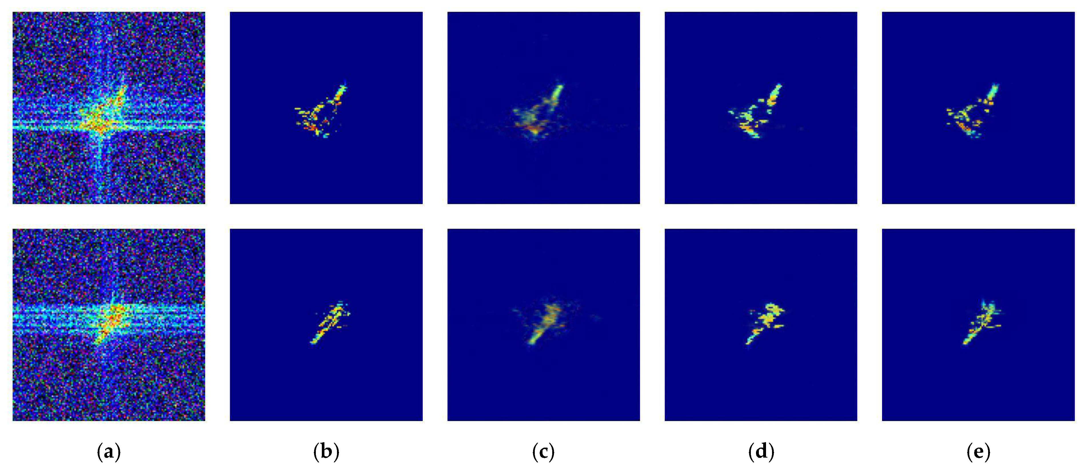
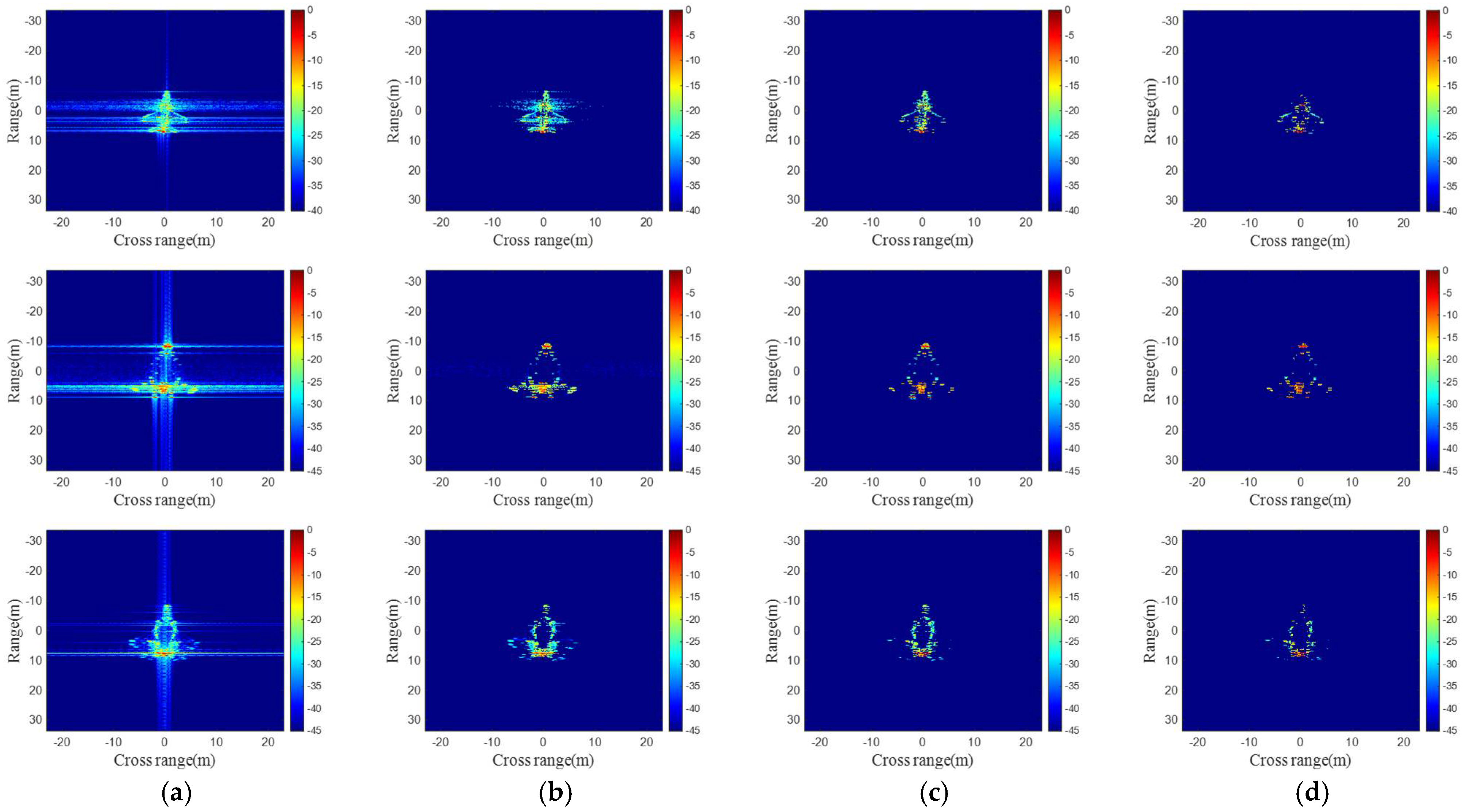
5. Simulation and Performance Evaluation

5.1. Introduction of the Datasets

This paper is structured into two datasets. The first dataset comprises electromagnetic simulation data, utilized to validate the network’s noise reduction performance under conditions of ample data. The second dataset combines a point scattering center model and electromagnetic simulation data, intended for evaluating the noise reduction efficacy in scenarios with limited data.

The parameters for constructing the first training set, a pure CAD model dataset, are as follows: the pitch plane spans from ${80}^{\circ }$ to ${120}^{\circ }$ in $5^{\circ }$ intervals, totaling nine pitch planes. The azimuth angle ranges from $1^{\circ }$ to ${360}^{\circ }$ degrees with an $1^{\circ }$ interval, resulting in 360 azimuths. The input set accumulates angles at $3^{\circ }$, with a bandwidth of 1 GHz, while the output set accumulates angles at $5^{\circ }$, with a bandwidth of 2 GHz. The training set comprises images from the pitch surface of ${90}^{\circ }\text{~}{120}^{\circ }$, resulting in a total of $360\times 7=2520$ images, while the output set includes pitch surfaces of 80 and 85 degrees, totaling $360\times 2=720$ images. Following imaging, the images are compressed to a size of $3\times 256\times 256$.

The second training set is a hybrid dataset, generated using the method proposed in Section 3. It includes 6000 scattering center simulation images as the pre-training set. The post-training set consists of three pitch planes (${110}^{\circ }\text{~}{120}^{\circ }$). Among them, 6000 scattering center images and data from pitch planes ${110}^{\circ }$ and ${115}^{\circ }$ are used as the training set, while the ${120}^{\circ }$ pitch plane serves as the test set. Similar to the first training set, the images are all of size $3\times 256\times 256$.

5.2. Evaluation Criterions

In line with the evaluation criteria in most papers for the image denoising effect, we used the peak signal-to-noise ratio (PSNR) and structural similarity (SSIM). The PSNR is often used as a measurement method for signal reconstruction quality in image compression and other fields. It is often simply defined as the mean square error (MSE). For two m × n monochromatic images I and K, if one is the noise approximation of the other, then their MSE is defined as

$$MSE=\frac{1}{mn}{\displaystyle \sum _{i=0}^{m-1}{\displaystyle \sum _{j=0}^{n-1}{\left[I(i,j)-K(i,j)\right]}^2}}$$

(23)

The PSNR is

$$PSNR=10\cdot {\log }_{10}\left(\frac{MA{X}_I^2}{MSE}\right)=20\cdot {\log }_{10}\left(\frac{MA{X}_I}{\sqrt{MSE}}\right)$$

(24)

where $MA{X}_I$ is the maximum value representing the color of the image point. If each sampling point is represented by 8 bits, it is 255. A more general representation is that if each sampling point is represented by a B-bit linear pulse code modulation, then $MA{X}_I$ is

$$MA{X}_I=2^B-1$$

(25)

For color images with three values at each point, the definition of the peak signal-to-noise ratio is similar, except that the mean square error is the sum of all variances divided by the image size and then divided by 3.

SSIM is another indicator to measure the similarity of two images. Similar to the PSNR, for two m × n monochromatic images I and K, the SSIM of the two images can be derived as follows,

$$SSIM(I,K)=\frac{(2{\mu }_I{\mu }_K+c_1)(2{\sigma }_{IK}+c_2)}{({\mu }_I^2+{\mu }_K^2+c_1)({\sigma }_I^2+{\sigma }_K^2+c_2)}$$

(26)

where ${\mu }_I$ is the mean value of I; ${\mu }_I^2$ denotes the variance of I, it has the same meaning if $I=K$. ${\sigma }_{IK}$ is the covariance between I and K. $c_1={(k_{1}L)}^2$, $c_2={(k_{2}L)}^2$ are the constants used to maintain stability. L means the dynamic range of the pixel value. $k_1=0.01$ and $k_1=0.03$.

5.3. Implementation Details

Table 4. The experimental environment.

Configuration	Parameter
CPU	Intel(R) Xeon(R) Platinum 8270 32-Core Processor
GPU	NVIDIA Quadro RTX 8000
Development tools	Python 3.10.8, Pytorch 1.13.1

describes the experimental environment described in this paper.

The batch size is set to 32 and the number of training epochs for datasets is 201. We used an Adam optimizer, with an initial learning rate of 0.01.

5.4. The Results of Training

(1) The result of CAD model dataset training.

In this paper, we introduce the spatially sparse attention module and loss function into three different network structures for processing ISAR images: the CNN-based network DNCNN, the encoder–decoder-based noise reduction network practical mobile raw image denoising network (PMRID-Net) [37], and the U-Net network-based pyramid real image denoising network (PRID-Net) [38]. These network structures are demonstrated in the Appendix A. Additionally, without loss of generality, to assess the advantages and disadvantages of the traditional processing method and the network processing method, we use the windowing function and the proposed ISAR processing flow as a control group. We conducted experiments at different side-lobe noise intensities, and the experimental comparison results are presented in Figure 16, Figure 17 and Figure 18, and the PSNRs and SSIMs for the three networks are summarized in

Table 5. The PSNR and SSIM values of the three networks.

Network	PSNR	SSIM
Improved DNCNN	29.20	0.9617
Improved PMRID-Net	30.01	0.9705
Improved PRID-Net	32.38	0.9784

.

The processing results corresponding to the azimuths ${103}^{\circ }$ to ${106}^{\circ }$ at a pitch angle of ${80}^{\circ }$ are shown in Figure 16, Figure 17 and Figure 18. In Figure 16, Figure 17 and Figure 18, (a) is the input image, (b) and (c) depict the conventional side-lobe noise cancellation method, while (d), (e), and (f) display the results of network processing. The results of each iteration of network processing are the same, and the simulation results are analyzed in Figure 18 as an example. From the simulation diagrams in Figure 18a–c, it is evident that the proposed ISAR imaging processing flow effectively reduces side-lobe noise and produces high-quality imaging results. However, due to the use of the fast clean algorithm, some weak scattering features lower than the side-lobe noise cannot be recovered in certain range bins, leading to the loss of information in the final processing results for this part. Furthermore, the abundance of point features in the target image makes such issues more difficult when employing the traditional point-to-point clean method.

Analyzing Figure 18d–f reveals that the network’s outputs offer a more comprehensive description of the target’s contour and provide richer image features, particularly regarding wing position information. Upon assessing the completeness of image features, it becomes evident that the processing results of the U-Net-based (Figure 18f) network and encoder–decoder-based network (Figure 18e) surpass those of the CNN-based network (Figure 18d). This can be attributed to the emphasis of the CNN network on local target features, resulting in insufficient feature extraction in non-attended regions and subsequent feature loss. Furthermore, in terms of resolution analysis, both the U-Net-based network and CNN-based network outperform the encoder–decoder-based network. This superiority can be attributed to the point-by-point analysis method employed by the U-Net and CNN networks, while the encoder–decoder structure focuses more on the correlation of each data line. It is clear that the point-by-point approach holds an advantage over the line-by-line method. This conclusion is reinforced with the results depicted in the figures. Finally, the comparison in Table 5 indicates that the U-Net-based network outperforms the CNN-based and encoder–decoder-based networks in terms of the PSNR and SSIM. Therefore, the U-Net-based network is deemed more suitable for ISAR noise reduction work.

The comparison between Figure 18c,f demonstrates that using the network for processing ISAR images yields superior results in the range bin containing weak scattering features. By comparing the processing methods, it is evident that the fast clean algorithm employs a bin-to-bin judgment, whereas the network utilizes a point-to-point judgment. The fast clean algorithm also utilizes a hard threshold as the index judgment, while the network adopts the feature method judgment. These distinct processing methods and judgment indexes contribute to the network-based processing method’s superior performance over the traditional processing method.

(2) The result of limited model dataset training.

In this section, our focus is on verifying the noise reduction effect of the three types of models under small-sample conditions and confirming the feasibility of enhancing the noise reduction effect through model migration. The first set of experiments involves training 200 times on a dataset constructed with limited electromagnetic scattering data. For the second set of experiments, the first 150 trials consist of training on a dataset constructed with the scattering center model, and the subsequent 50 trials involve training on the electromagnetic scattering dataset. The PSNR and the number of training sessions corresponding to the best training results achieved by the two training methods are presented in

Table 6. The experiment results.

Network	1st Experiment		2nd Experiment
	PSNR	Epoch	PSNR	Epoch
Improved DNCNN	25.15	200	27.76	50
Improved PMRID-Net	27.05	176	28.26	42
Improved PRID-Net	30.16	152	30.33	28

.

Comparing Table 5 and Table 6, it is evident that the noise reduction effect of the network diminishes as the data volume decreases, leading to a reduction in the PSNR by 2 dB. This is attributed to the insufficient extraction of image features by the network under conditions of limited samples, resulting in reduced classification accuracy of target features and noise, consequently hindering the achievement of high-precision side-lobe noise reduction.

Furthermore, when comparing the two training strategies, the second training method enhances the noise reduction effect, particularly evident in the improvement of the DNCNN. This improvement stems from the critical role of the initial value setting in the training process of convolutional networks. Pre-training based on the scattering center model provides an effective descent direction for subsequent training, thereby enhancing training accuracy. As for the other two networks, the increase in model complexity reduces the required number of training sessions. However, the change in training strategy does not effectively enhance the network noise reduction accuracy, resulting in similar training outcomes for both methods. Nevertheless, the second method’s provision of a good initial value drastically reduces the number of training sessions required to achieve the final result, effectively improving training efficiency.

(3)The results of different signal-to-noise ratios (SNRs).

To further evaluate the robustness of the network, we have constructed a dataset that includes two different targets. The construction of the input and output datasets follows the same method as in Section 5.4(1). Additionally, after the dataset is completed, we introduce 0 dB Gaussian white noise during the training and testing phases and resize the images to $3\times 128\times 128$ to assess the model’s noise reduction capabilities under various conditions. The CAD images of the targets are illustrated in Figure 3, and the simulation results under different signal-to-noise ratios (SNRs) are presented in Figure 19, Figure 20 and Figure 21.

In Figure 19, Figure 20 and Figure 21, we present the side-lobe noise reduction performance of three networks under varying signal-to-noise ratios (SNRs) of −5, 0, and 5 dB. As evident from the figures, both the improved PMRID-Net and the improved PRID-Net demonstrate robust noise reduction capabilities across all three SNR levels. Conversely, the DNCNN only functions effectively under an SNR of 0 dB or below. Notably, under these challenging conditions, while the PSNR and convergence speed of all three networks exhibit a relative decrease compared to the experiment in Section 5.4(1), they nevertheless maintain a stable capacity to outline the target contours. This observation validates the noise reduction performance of these networks, even under low SNR scenarios.

(4) Ablation Studies.

Finally, we validated the impact of the spatial attention module and the enhanced loss function proposed in this paper on the network training accuracy, and the results are presented in

Table 7. The ablation study of three models.

Network	PSNR
Improved DNCNN	29.20
DNCNN	27.26
Improved PMRID-Net	30.01
PMRID-Net	28.65
Improved PRID-Net	32.38
PRID-Net	31.65

.

As shown in Table 7, the proposed improvement method in this paper results in enhancements across all three networks, with the most significant performance improvement observed with the DNCNN with a 1.98 dB increase in the PSNR, followed by a 1.36 dB improvement for PMRID-Net, and a 0.68 dB improvement for PRID-Net. This can be attributed to the fact that networks based on the encoder–decoder structure and the U-Net structure inherently possess spatial attention capabilities, while the CNN structure lacks such capabilities, hence yielding the best performance in DNCNN.

In another ablation experiment, we aimed to investigate the impact of threshold values on the performance of the fast clean algorithm for ISAR imaging. Specifically, we conducted ISAR imaging of three targets under the conditions of a 2 GHz bandwidth, a 6° accumulation angle, and a 120° elevation plane. For the fast clean algorithm, the threshold values are 0, 1, and 5. The imaging results are shown in Figure 22.

As illustrated in Figure 22, the effect of threshold values on the imaging results is significant. When the threshold is set low, as seen in Figure 22b, it is unable to completely remove the side-lobe noise from the image. Conversely, when the threshold is set high, as depicted in Figure 22d, it can lead to the loss of valuable information. Therefore, selecting an appropriate threshold is crucial for enhancing image quality.

Moreover, from Figure 22a, it is evident that the side-lobe noise in the range dimension is significantly higher than in the cross-range dimension. Taking this observation into consideration, as well as the comprehensive simulations performed in this study, the final parameter choice for the threshold, ${\alpha }_1=5,{\alpha }_2=1$, was determined.

6. Conclusions

As for undergoing the ISAR imaging tasks, the imaging quality deteriorates when the side-lobe noise exceeds the level of weak scattering points. To address this issue, this paper employs a deep learning approach. By designing a fast clean algorithm, introducing a spatial attention module, and improving the loss function, the existing noise reduction network can be repurposed for ISAR side-lobe noise reduction. Additionally, in order to address the challenges of side-lobe noise reduction under limited sample conditions, this paper also explores a training method based on model migration, which enhances training accuracy under the restricted dataset conditions. Finally, the effectiveness of the proposed method is demonstrated through verification on the dataset designed in this paper.

However, there persist a few challenges in the research on side-lobe noise reduction. Firstly, network-based noise reduction techniques are inherently dependent on the dataset. In scenarios where the target structures exhibit similar characteristics, the networks can deliver satisfactory noise reduction outcomes. However, in cases where significant structural differences are present, the results often fail to meet expectations.

Secondly, the evaluation criterion poses another obstacle. While this study employs the PSNR as an indicator to assess the network’s noise reduction performance, this metric, originally designed for optical image processing, is not entirely suitable for ISAR images. The PSNR focuses primarily on the consistency between the input and output images, but we cannot guarantee that the output provided by the network is indeed the optimal outcome. Our goal is to enable the network to achieve superior results through continuous learning.

In future work, we plan to delve deeper into both of these aspects. We aim to develop more robust and adaptive network architectures that can handle structural variations more effectively. Additionally, we will explore alternative evaluation criteria that are more tailored to the characteristics of ISAR images, enabling a more accurate assessment of the network’s noise reduction performance.

References

1. Bhanu, B.; Dudgeon, D.E.; Zelnio, E.G.; Rosenfeld, A.; Casasent, D.; Reed, I.S. Guest editorial introduction to the special issue on automatic target detection and recognition. IEEE Trans. Image Process. 1997, 6, 1–6. [Google Scholar] [CrossRef]
2. Meng, H.; Peng, Y.; Wang, W.; Cheng, P.; Li, Y.; Xiang, W. Spatio-Temporal-Frequency graph attention convolutional network for aircraft recognition based on heterogeneous radar network. IEEE Trans. Aerosp. Electron. Syst. 2022, 58, 5548–5559. [Google Scholar] [CrossRef]
3. Gao, G. An improved scheme for target discrimination in high-resolution SAR images. IEEE Trans. Geosci. Remote Sens. 2011, 49, 277–294. [Google Scholar] [CrossRef]
4. Marchetti, E.; Stove, A.G.; Hoare, E.G.; Cherniakov, M.; Blacknell, D.; Gashinova, M. Space-based sub-THz ISAR for space situational awareness—Concept and design. IEEE Trans. Aerosp. Electron. Syst. 2022, 58, 1558–1573. [Google Scholar] [CrossRef]
5. Berizzi, F.; Mese, E.D.; Diani, M.; Martorella, M. High-resolution ISAR imaging of maneuvering targets by means of the range instantaneous Doppler technique: Modeling and performance analysis. IEEE Trans. Image Process. 2001, 10, 1880–1890. [Google Scholar] [CrossRef] [PubMed]
6. Wehner, D.R. High Resolution Radar; Artech House: Norwood, MA, USA, 1987. [Google Scholar]
7. Jakowatz, C.V.; Wahl, D.E.; Eichel, P.H.; Ghiglia, D.C.; Thompson, P.A. Spotlight-Mode Synthetic Aperture Radar: A Signal Processing Approach; Kluwer: Boston, MA, USA, 1996. [Google Scholar]
8. Harris, F.J. On the use of windows for harmonic analysis with the discrete Fourier transform. Proc. IEEE 1978, 66, 51–83. [Google Scholar] [CrossRef]
9. Kulkarni, R.G. Polynomial Windows with fast decaying sidelobes for narrow-band signals. Signal Process. 2003, 83, 1145–1149. [Google Scholar] [CrossRef]
10. Yoon, T.H.; Joo, E.K. A Flexible Window Function for Spectral Analysis [DSP Tips & Tricks]. IEEE Signal Process. Mag. 2010, 27, 139–142. [Google Scholar]
11. Tsao, J.; Steinberg, B.D. Reduction of sidelobe and speckle artifacts in microwave imaging: The CLEAN technique. IEEE Trans. Antennas Propag. 1988, 36, 543–556. [Google Scholar] [CrossRef]
12. Choi, I.-S.; Kim, H.-T. Two-dimensional evolutionary programming-based CLEAN. IEEE Trans. Aerosp. Electron. Syst. 2003, 39, 373–382. [Google Scholar] [CrossRef]
13. Zhang, K.; Zuo, W.; Chen, Y.; Meng, D.; Zhang, L. Beyond a Gaussian Denoiser: Residual Learning of Deep CNN for Image Denoising. IEEE Trans. Image Process. 2017, 26, 3142–3155. [Google Scholar] [CrossRef] [PubMed]
14. Guo, S.; Yan, Z.; Zhang, K.; Zuo, W.; Zhang, L. Toward Convolutional Blind Denoising of Real Photographs. In Proceedings of the 2019 IEEE/CVF Conference on Computer Vision and Pattern Recognition (CVPR), Long Beach, CA, USA, 15–20 June 2019; pp. 1712–1722. [Google Scholar]
15. Yu, K.; Wang, X.; Dong, C.; Tang, X.; Loy, C.C. Path-Restore: Learning Network Path Selection for Image Restoration. IEEE Trans. Pattern Anal. Mach. Intell. 2022, 44, 7078–7092. [Google Scholar] [CrossRef] [PubMed]
16. Mao, X.J.; Shen, C.H.; Yang, Y.B. Image restoration using very deep convolutional encoder-decoder networks with symmetric skip connections. In Proceedings of the 30th International Conference on Neural Information Processing Systems (NIPS), Barcelona, Spain, 5–10 December 2016; pp. 2802–2810. [Google Scholar]
17. Jin, S.; Bae, Y.; Lee, S. ID-SAbRUNet: Deep Neural Network for Disturbance Suppression of Drone ISAR Images. IEEE Sens. J. 2024, 24, 15551–15565. [Google Scholar] [CrossRef]
18. Walker, J.L. Range-Doppler Imaging of Rotating Objects. IEEE Trans. Aerosp. Electron. Syst. 1980, AES-16, 23–52. [Google Scholar] [CrossRef]
19. Ausherman, D.A.; Kozma, A.; Walker, J.L.; Jones, H.M.; Poggio, E.C. Developments in Radar Imaging. IEEE Trans. Aerosp. Electron. Syst. 1984, AES-20, 363–400. [Google Scholar]
20. Yu, X.; Wang, Z.; Du, X.; Jiang, L. Multipass Interferometric ISAR for Three-Dimensional Space Target Reconstruction. IEEE Trans. Geosci. Remote Sens. 2022, 60, 5110317. [Google Scholar] [CrossRef]
21. Chang, S.; Deng, Y.; Zhang, Y.; Zhao, Q.; Wang, R.; Zhang, K. An Advanced Scheme for Range Ambiguity Suppression of Spaceborne SAR Based on Blind Source Separation. IEEE Trans. Geosci. Remote Sens. 2022, 60, 5230112. [Google Scholar] [CrossRef]
22. Çulha, O.; Tanık, Y. Efficient Range Migration Compensation Method Based on Doppler Ambiguity Shift Transform. IEEE Sens. Lett. 2022, 6, 7000604. [Google Scholar] [CrossRef]
23. Chen, C.-C.; Andrews, H.C. Target-Motion-Induced Radar Imaging. IEEE Trans. Aerosp. Electron. Syst. 1980, AES-16, 2–14. [Google Scholar] [CrossRef]
24. Itoh, T.; Sueda, H.; Watanabe, Y. Motion compensation for ISAR via centroid tracking. IEEE Trans. Aerosp. Electron. Syst. 1996, 32, 1191–1197. [Google Scholar] [CrossRef]
25. Zhu, D.; Wang, L.; Yu, Y.; Tao, Q.; Zhu, Z. Robust ISAR Range Alignment via Minimizing the Entropy of the Average Range Profile. IEEE Geosci. Remote Sens. Lett. 2009, 6, 204–208. [Google Scholar]
26. Wang, J.F.; Kasilingam, D. Global range alignment for ISAR. IEEE Trans. Aerosp. Electron. Syst. 2003, 39, 351–357. [Google Scholar] [CrossRef]
27. Yang, J.G.; Huang, X.T.; Jin, T.; Xue, G.Y.; Zhou, Z.M. An Interpolated Phase Adjustment by Contrast Enhancement Algorithm for SAR. IEEE Geosci. Remote Sens. Lett. 2011, 8, 211–215. [Google Scholar]
28. Perry, R.P.; DiPietro, R.C.; Fante, R.L. SAR imaging of moving targets. IEEE Trans. Aerosp. Electron. Syst. 1999, 35, 188–200. [Google Scholar] [CrossRef]
29. Song, Y.; Pu, W.; Huo, J.; Wu, J.; Li, Z.; Yang, J. Deep Parametric Imaging for Bistatic SAR: Model, Property, and Approach. IEEE Trans. Geosci. Remote Sens. 2024, 62, 5212416. [Google Scholar] [CrossRef]
30. Xiao-Yu, X.; Huo, Y.; Hong-Cheng, C.-Y.Y. Performance Analysis for Two Parameter Estimation Methods of GTD Model. In Proceedings of the 2018 IEEE International Conference on Computational Electromagnetics (ICCEM), Chengdu, China, 26–28 March 2018; pp. 1–3. [Google Scholar]
31. Potter, L.C.; Chiang, D.-M.; Carriere, R.; Gerry, M.J. A GTD-based parametric model for radar scattering. IEEE Trans. Antennas Propag. 1995, 43, 1058–1067. [Google Scholar] [CrossRef]
32. Potter, L.C.; Moses, R.L. Attributed scattering centers for SAR ATR. IEEE Trans. Image Process. 1997, 6, 79–91. [Google Scholar] [CrossRef]
33. Sketchfab 3D Resource. Available online: https://sketchfab.com/ (accessed on 24 November 2023).
34. Wang, Z.; Fu, Y.; Liu, J.; Zhang, Y. LG-BPN: Local and Global Blind-Patch Network for Self-Supervised Real-World Denoising. In Proceedings of the 2023 IEEE/CVF Conference on Computer Vision and Pattern Recognition (CVPR), Vancouver, BC, Canada, 18–22 June 2023; pp. 18156–18165. [Google Scholar]
35. Zhang, Y.; Wang, R. A novel high-resolution and wide-swath SAR imaging mode. In Proceedings of the 13th European Conference on Synthetic Aperture Radar (EUSAR), Online, 29 March–1 April 2021; pp. 1–6. [Google Scholar]
36. Chen, X.; Wang, Z.J.; Mckeown, M. Joint blind source separation for neurophysiological data analysis: Multiset and multimodal methods. IEEE Signal Process. Mag. 2016, 33, 86–107. [Google Scholar] [CrossRef]
37. Wang, Y.; Huang, H.; Xu, Q.; Liu, J.; Liu, Y.; Wang, J. Practical Deep Raw Image Denoising on Mobile Devices. In 2020 European Conference on Computer Vision (ECCV); Springer: Cham, Switzerland, 2020; Volume 12351. [Google Scholar]
38. Zhao, Y.; Jiang, Z.; Men, A.; Ju, G. Pyramid Real Image Denoising Network. In Proceedings of the 2019 IEEE Visual Communications and Image Processing (VCIP), Sydney, NSW, Australia, 1–4 December 2019; pp. 1–4. [Google Scholar]
Figure 1. The ISAR image of the 1st experiment with different ε I . (a) ε I = 30 dB and (b) ε I = 15 dB.
Remotesensing 16 02279 g001
Figure 2. The ISAR image of the 2nd experiment with different ε I . (a) ε I = 30 dB and (b) ε I = 25 dB.
Remotesensing 16 02279 g002
Figure 3. The CAD model of two targets. (a) non-stealth structure aircraft (target 1) and (b) stealth structure aircraft (target 2).
Remotesensing 16 02279 g003
Figure 4. The ISAR images of target 1 with θ from 0 to 5 and φ = 120 with different ε I values. (a) ε I = 40 dB and (b) ε I = 30 dB.
Remotesensing 16 02279 g004
Figure 5. The ISAR images of target 1 with θ from 99 to 104 and φ = 120 with different ε I values. (a) ε I = 40 dB and (b) ε I = 30 dB.
Remotesensing 16 02279 g005
Figure 6. The ISAR images of target 1 with θ from 36 to 41 and φ = 120 with different ε I values. (a) ε I = 40 dB and (b) ε I = 30 dB.
Remotesensing 16 02279 g006
Figure 7. The ISAR images of the stealth targets with θ from 0 to 5 and φ = 120 with different ε I values. (a) ε I = 40 dB and (b) ε I = 30 dB.
Remotesensing 16 02279 g007
Figure 8. The ISAR images of Space Shuttle Atlantis in different observation angles.
Remotesensing 16 02279 g008
Figure 9. Examples of denoising operations. (a) An example of rain denoising. (b) An example of side-lobe denoising.
Remotesensing 16 02279 g009
Figure 10. The flow chart of this paper.
Remotesensing 16 02279 g010
Figure 11. The architecture of the spatial attention block.
Remotesensing 16 02279 g011
Figure 12. The input and output images. (a,c,e,g) are the input ISAR images. (b,d,f,h) are the output ISAR images.
Remotesensing 16 02279 g012aRemotesensing 16 02279 g012b
Figure 13. The schematic diagram of the coordinate system.
Remotesensing 16 02279 g013
Figure 14. The flight trajectory. h is the flight height, s is route shortcut, v means flight speed, t denotes accumulation time, r represents flight distance, and θ 1 , θ 2 is the starting and ending azimuth angle, respectively.
Remotesensing 16 02279 g014
Figure 15. The input and output images based on the electromagnetic simulation model. (a,c,e,g) are the input ISAR images. (b,d,f,h) are the output ISAR images.
Remotesensing 16 02279 g015
Figure 16. The result of side-lobe denoising using different methods for weak side-lobe noise; (a) the input image, (b) the result using the window function, (c) the result using the ISAR image flow proposed in this paper, (d) the result using the improved DNCNN, (e) the result using the improved PMRID-Net, and (f) the result using the improved PRID-Net.
Remotesensing 16 02279 g016
Figure 17. The result of side-lobe denoising using different methods for side-lobe noise; (a) the input image, (b) the result using the window function, (c) the result using the ISAR image flow proposed in this paper, (d) the result using the improved DNCNN, (e) the result using the improved PMRID-Net, and (f) the result using the improved PRID-Net.
Remotesensing 16 02279 g017
Figure 18. The result of side-lobe denoising using different methods for strong side-lobe noise; (a) the input image, (b) the result using the window function, (c) the result using the ISAR image flow proposed in this paper, (d) the result using the improved DNCNN, (e) the result using the improved PMRID-Net, and (f) the result using the improved PRID-Net.
Remotesensing 16 02279 g018
Figure 19. The result of side-lobe denoising using different methods with a SNR = −5 dB; (a) the input image with noise, (b) the ideal output image, (c) the result using the improved DNCNN, (d) the result using the improved PMRID-Net, and (e) the result using the improved PRID-Net. The colour here indicates the relative magnitude, the darker the colour the higher the magnitude.
Remotesensing 16 02279 g019
Figure 20. The result of side-lobe denoising using different methods with a SNR = 0 dB; (a) the input image with noise, (b) the ideal output image, (c) the result using the improved DNCNN, (d) the result using the improved PMRID-Net, and (e) the result using the improved PRID-Net. The colour here indicates the relative magnitude, the darker the colour the higher the magnitude.
Remotesensing 16 02279 g020
Figure 21. The result of side-lobe denoising using different methods with a SNR = 5 dB; (a) the input image with noise, (b) the ideal output image, (c) the result using the improved DNCNN, (d) the result using the improved PMRID-Net, and (e) the result using the improved PRID-Net. The colour here indicates the relative magnitude, the darker the colour the higher the magnitude.
Remotesensing 16 02279 g021
Figure 22. The output ISAR images of different targets using the fast clean algorithm with different thresholds; (a) The output ISAR images using the fast clean algorithm with α 1 = 0 , α 2 = 0 , (b) the output ISAR images using the fast clean algorithm with α 1 = 1 , α 2 = 1 , (c) the output ISAR images using the fast clean algorithm with α 1 = 5 , α 2 = 1 , and (d) the output ISAR images using the fast clean algorithm with α 1 = 5 , α 2 = 5 .
Remotesensing 16 02279 g022