Monitoring CH₄ Fluxes in Sewage Sludge Treatment Centres: Challenging Emission Underreporting

Abstract

In this manuscript, CH₄ emissions from sludge treatment centres are quantified using an unmanned aerial vehicle (UAV) framework, with particular focus on anaerobic digesters and digestate storage tanks. The outcomes are compared to those obtained using the carbon accounting workbook (CAW), which is the most commonly used industry tool by UK and Irish water companies to estimate the annual greenhouse gas emissions from their process operations. Path integrated concentrations are monitored with the use of an open-path tuneable diode laser absorption spectroscopy sensor embedded on a UAV. Measurements are interpolated using geostatistics (Kriging) and coupled with the mass balance approach to estimate emissions. The findings show that the CAW seems to underestimate emissions from digestate storage tanks by up to an order of magnitude. The results also show that CH₄ emissions are linked with the residence time in the tank and temperature of the digestate. This study highlights the limitations of assumptions made using current reporting methods based on the carbon accounting workbook. This study proves that the UAV framework, together with the mass balance approach, provides high spatial resolution data; it captures the dynamic nature of emissions compared to the CAW and can be a cost-effective solution to estimate CH₄ fluxes compared to other sensor-based systems.

1. Introduction

With the increasing trend of the global average temperature, concerns have arisen regarding mitigating efforts. Global initiatives and agreements have been initiated to mitigate climate change’s impact. The Paris agreement aims at limiting the temperature increment to below 2 °C [1] and achieving net zero carbon emission by 2050 [2]. In 2019, UK water companies made commitments to reduce greenhouse gas (GHG) emissions and to progress towards net zero targets [2]. Scope 1 emissions, which are direct GHG emissions caused by sources owned or controlled by the company, usually receive particular attention. Wastewater treatment plants (WWTPs) are major sources of methane (CH₄) and nitrous oxide (N₂O), which have global warming potentials (GWP-100) of 27.2 and 273 over a 100-year horizon, respectively [3,4]. Within WWTPs, the wastewater treatment (WWT) line is primarily a source of N₂O, as aerobic conditions are maintained in part of the treatment process [5]. In contrast, treatment of the sludge generated during wastewater treatment is a major CH₄ source due to the anaerobic conditions governing the processes. The atmospheric lifetimes for CH₄ and N₂O are approximately a decade and 114 years, respectively [6]. The reduction in gases with short lifetimes leads to a more rapid reduction in the global average temperature increment, driven by the lag between the reduction in emissions and the reduction in atmospheric concentration. Therefore, reducing CH₄ emissions would be more effective to manage temperature increments in the short term than to reduce N₂O [7]. This study focuses on quantifying CH₄ emissions from sludge treatment centres.

Water utilities in the UK currently rely on the carbon accounting workbook (CAW) to estimate and report their GHG emissions [8]. In the European Union, wastewater and sludge treatment facilities must report their environmental emissions to the European Pollutant Release and Transfer Register if they surpass a specified threshold. The reporting pollutant threshold for CH₄ is 100,000 kg yr⁻¹ to air [9]. Guidelines outlined by the International Panel on Climate Change (IPCC) dictate the reporting of these emissions [10]. With regard to CH₄ emissions, these guidelines are based on the principle that CH₄ emissions are influenced by the organic matter present in waste and the emission factor, which indicates the potential of a specific asset to produce CH₄. The CAW defines a set of emission factors for different assets based on previous scientific studies [11,12,13,14,15] which closely monitored how variables such as flow rates, organic matter contents, chemical oxygen demands, and biological oxygen demands at both inlets and outlets of individual assets determine the potential to emit GHGs. In the CAW, these emission factors are normalised over the amount of incoming dry solids to the plant by incorporating correction factors suggested by the IPCC [8]. The CAW utilizes these emission factors and enables the estimation of CH₄ fluxes based on the volume of sludge treated and the type of treatment employed. The current methodology, based on default emission factors, has limitations that curtail its accuracy and reliability. The potential of sludge to emit CH₄ depends on many environmental factors, such as temperature and humidity; WWTP operational factors, such as sludge inflow, amount of organic degradable matter [5], and asset operational conditions; and maintenance of leaks in digesters and pipelines.

Previous literature has highlighted that emission factors are plant- and asset-specific. Delre et al. [10] and Daelman et al. [12] stated that CH₄ is lower in WWTPs with enclosed sludge treatment lines, with diurnal and seasonal variations in CH₄ emissions which sometimes do not correlate well with the influent flow rate. CH₄ emissions from digestate storage tanks are also inversely correlated to the sludge retention time in the anaerobic digester. The accuracy of currently available emission factors also greatly depends on the type of assets on site. The development of frameworks with actual site-based data sets is therefore recommended by the CAW [8]. In turn, this generates the need to define suitable CH₄ quantification techniques.

Emissions from closed assets, such as leaks from anaerobic digesters and pipelines, tend to fall under “point source” emissions and pose a challenge for identification, but can frequently be measured once found. Contrarily, “open source” emissions tend to be identifiable, but it is particularly challenging to quantify their emission fluxes, as these originate from large areas and can exhibit high spatio-temporal variability. This is the case for digestate storage tanks, for which emission quantification can be challenging due to variations driven by factors such as heterogeneous mixing of digestate, variations in digestate filling level, and digestate temperature dependency on the ambient air temperature [16].

Recent studies have estimated CH₄ emissions in WWTPs by coupling unmanned aerial vehicle (UAV)-based remote sensing methods with the mass balance approach [17,18]. One of the main advantages of remote sensing methods over more traditional approaches is that human access to the exact monitoring location is not required. The tracer gas dispersion method has recently been reported as an alternative method to estimate CH₄ fluxes from WWTPs [10]. However, this approach requires the release of a sufficient amount of tracer gas and the integration of sensors capable of measuring both CH₄ and the tracer gas concentrations on a UAV platform.

UAVs provide close-to-source monitoring capability with a single sensor, minimizing the accessibility risk whilst providing higher spatial resolution. From the two main types of UAVs available in the market (fixed wing and vertical take-off and landing (VTOL)), fixed wings require a deployment platform to take off and land, while VTOLs are capable of taking off and landing vertically. During flight, the flying altitude and direction can be easily controlled when it comes to VTOLs, which are also capable of hovering over a specific location. The use of VTOLs for CH₄ monitoring is limited by the weight and dimensions of the sensor. Recent developments in sensor technology have allowed some of these limitations to be overcome by the lightweight U10 (DJI, China) CH₄ sensor based on open-path, tunable diode laser absorption spectroscopy (TDLAS) [19].

Abeywickrama et al. [19] presented the first application of the U10 open-path TDLAS CH₄ sensor in a WWTP in England. This sensor can be embedded in specific DJI (DJI, China) UAV models and enables the measurement of CH₄ concentration along a gas column. The authors developed a framework detailing how to monitor asset-level CH₄ concentrations from anaerobic digesters, cake pads, and digestate storage tanks using a UAV platform, specifically the model Matrice RTK 300 DJI (DJI, China). The aim of this paper is to quantify differences in CH₄ flux estimation by comparing a UAV-U10-based mass balance approach with the CAW method for selected assets within a WWTP.

2. Materials and Methods

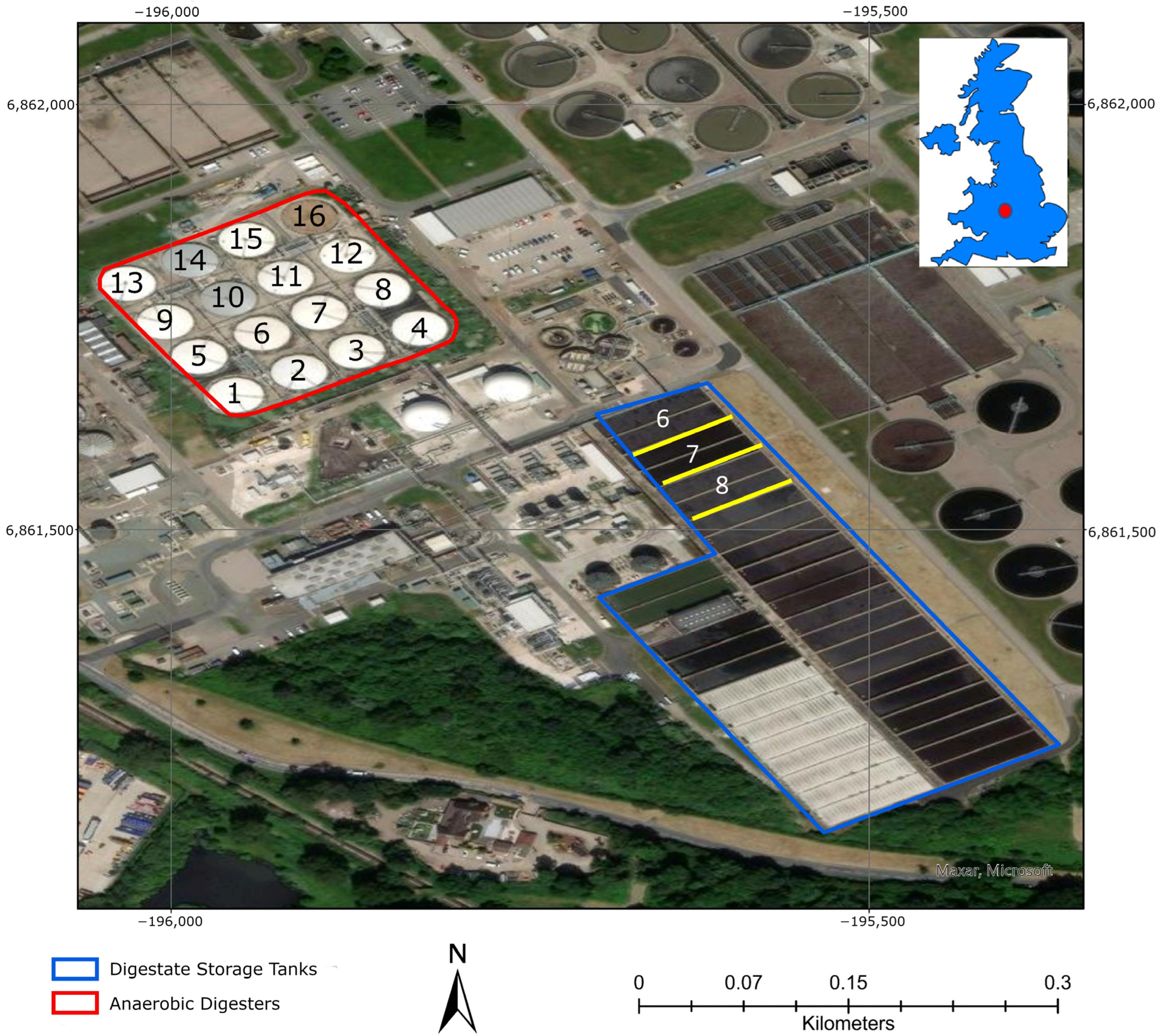
2.1. Case Study Area

A WWTP with a sludge treatment line in Minworth (West Midlands, UK), with a serving capability for a population equivalent of approximately 1.7 million [20], was selected as the case study area (Figure 1). The sludge treatment line within the WWTP treats 67,166 tDS yr⁻¹ in sixteen advanced anaerobic digesters, which are preceded by a thermal hydrolysis process (THP). Each anaerobic digester has a cylindrical shape with a diameter of approximately 26 m and floating roofs. The anaerobic digesters are contained in a 125 m × 125 m area, and the centres of each digester are 27 m apart from each other. Treated sludge (digestate) flows into sixteen digestate storage tanks, which are used as buffer tanks with an average of 1–2 days of retention time. The sludge is then dewatered and applied to land as an organic fertilizer. Each digestate storage tank comprises two bays separated by a concrete wall of interlinked arcs. The length and width of each digestate storage tank are 55 m and 26 m, respectively.

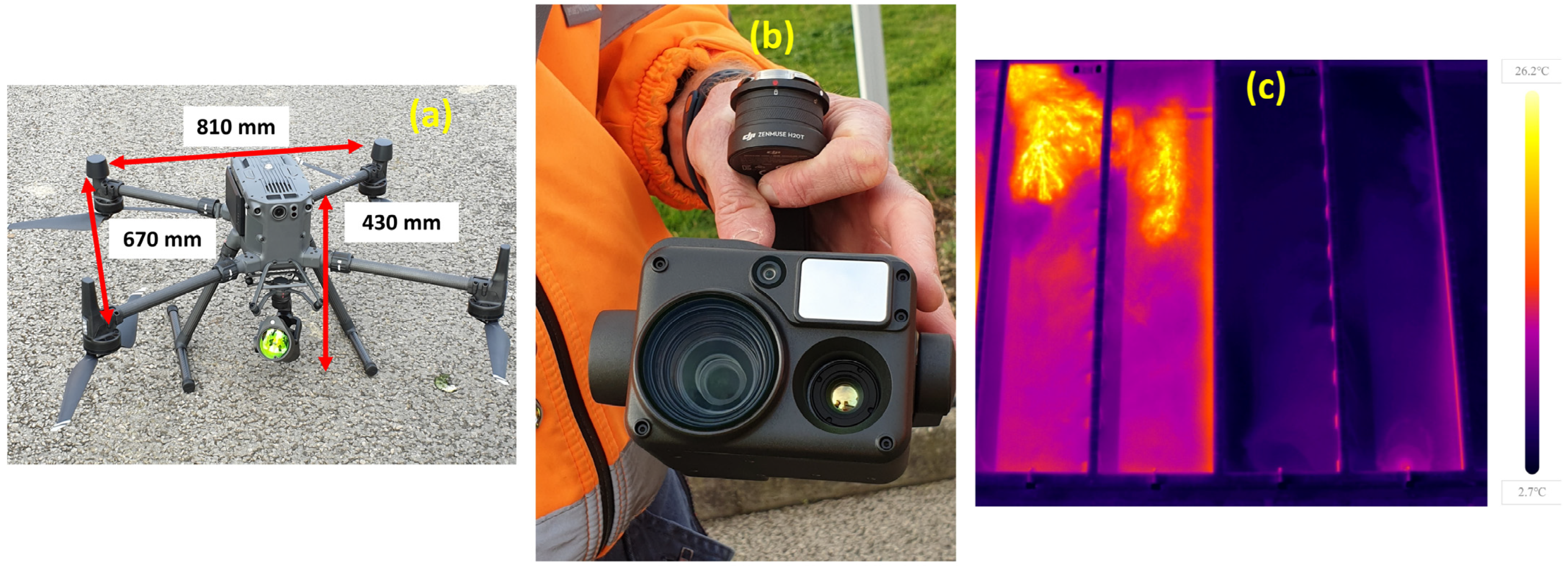
2.2. UAV Data Collection

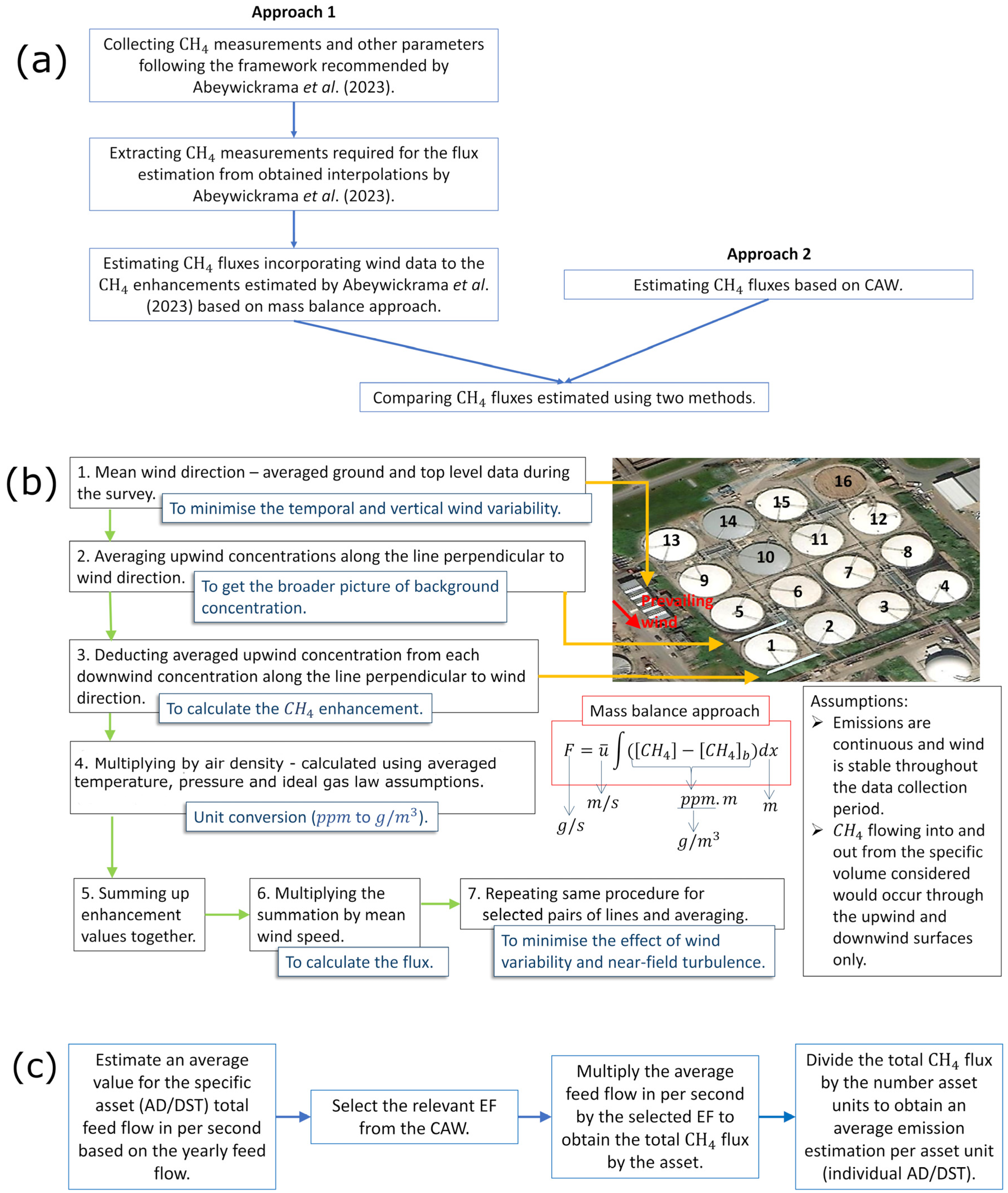
The U10 sensor mounted on the Matrice 300 RTK UAV (DJI, Shenzhen, China) was used to measure CH₄ concentrations (Figure 2) [19] from anaerobic digesters and digestate storage tanks. The U10 TDLAS sensor CH₄ measurements were based on Beer–Lambert’s Law [22]. The U10 threshold of detection was 5 ppm∙m, and concentrations below the threshold were not recorded by the system. The framework developed by Abeywickrama et al. [19] was followed at all times to gather the required data for both anaerobic digesters and digestate storage tanks. The UAV flight altitude above ground level remained constant through the duration of each mission at 30 m for the anaerobic digesters and 20 m for the digestate storage tanks.

Two surveys were conducted for the anaerobic digesters on 21 March 2022 (survey 1) and 18 May 2022 (survey 2). Multipasses overlaid in two directions were used to cover the extent of the surveyed area. Each survey covered as many digesters as possible under given weather conditions and operational constrains. Of the sixteen digesters, two were empty and not operational and, therefore, were excluded from all surveys. During survey 2, three digesters were surveyed in one direction, and another three were not surveyed due to UAV health and safety operational limitations. A total of eight digesters were surveyed in full during the first survey, whereas eleven were surveyed at least in one direction in the second survey.

The digestate storage tanks were surveyed on 4 November 2022 (survey 3). First, the UAV was flown across all digesters with a thermal camera DJI Zenmuse H20T (DJI, China) (Figure 2) to identify the tank with the highest emissions, as temperature has been linked to methanogenic activity in previous literature [23]. A detailed CH₄ survey was then conducted for that tank.

Several additional data sets were gathered (

Table 1. Summary of UAV data collected during each survey for the anaerobic digesters (AD) and the digestate storage tanks (DST). For the anaerobic digesters, mean values of temperature, pressure, relative humidity, wind speed, and direction per survey are presented along with their standard deviations. A single value of each parameter (WS, WD, T, RH, and P) was obtained for each flight. The mean values reported (and associated standard deviation) refer to the averaged value for all the flights carried out within a single survey. The standard deviation was not calculated for the DST, as only one flight was implemented. Wind direction is represented following UK Met Office format (e.g., northerly winds −360°, southerly winds −180°, westerly winds −270°, easterly winds −90°). $\overline{\mathrm{W}\mathrm{S}}$, $\overline{\mathrm{W}\mathrm{D}}$, $\overline{\mathrm{T}}$, $\overline{\mathrm{R}\mathrm{H}}$, and $\overline{\mathrm{P}}$ stand for mean wind speed, mean ground wind direction, mean ground temperature, ground relative humidity, and mean ground pressure, respectively. In this table, N denotes the number of CH₄ measurements recorded by the U10.

Asset	Survey Code	Date	N	Flights	$\overline{\mathbf{W}\mathbf{S}}$ (m s−1)	$\overline{\mathbf{W}\mathbf{D}}$ (°)	$\overline{\mathbf{T}}$ (°C)	$\overline{\mathbf{R}\mathbf{H}}$ (%)	$\overline{\mathbf{P}}$ (hPa)
AD	1	21 March 2021	3771	6	2.8 ± 0.4	150 ± 10	12.7 ± 0.7	59 ± 4	1025.8 ± 0.4
	2	18 May 2021	284	8	5.8 ± 0.9	194 ± 5	18.0 ± 1.4	58 ± 3	1018.3 ± 1.2
DST	3	4 November 2021	532	1	4.9	302	12.3	72	1013.8

), including wind speed and direction, temperature, pressure, and the U10 laser angle. All these variables were recorded using sensors integrated into the UAV platform, except for the U10 laser angle, which was maintained in nadir position at all times.

2.3. Data Analysis

Two approaches (Figure 3) were used to estimate CH₄ fluxes: the mass balance [24] and the CAW [8]. The following sections describe the key steps underlying each approach and how results were compared between approaches.

2.3.1. Mass Balance Approach

The mass balance approach considers the conservation of CH₄ mass within a system or volume. In brief, within a specific volume, the accumulation rate of CH₄ is the addition of CH₄ inflow to the volume and sources within the volume, from which the outflow and losses are subtracted (Figure 3). At steady state, the accumulation rate of CH₄ is equal to 0. The total emission (E) (g s⁻¹) for an infinitesimal area within the plane perpendicular to the wind can be estimated using Equation (1).

$$\begin{array}{c}\mathrm{E}=\left(\left[{\mathrm{C}\mathrm{H}}_4\right]-{\left[{\mathrm{C}\mathrm{H}}_4\right]}_{\mathrm{b}}\right)\mathrm{u}\mathrm{d}\mathrm{x}\mathrm{d}\mathrm{z}\end{array}$$

(1)

where $\left[{\mathrm{C}\mathrm{H}}_4\right]$ is the measurement of CH₄ concentration downwind of the plume (g m⁻³); ${\left[{\mathrm{C}\mathrm{H}}_4\right]}_{\mathrm{b}}$ is the background concentration, which is usually measured upwind of the source (g m⁻³); u is the wind speed (m s⁻¹) perpendicular to the vertical plane on which the plume is projected; and dx and dz are infinitesimal differences along the horizontal and vertical directions, respectively, of the plane perpendicular to the wind speed u (m).

The total flux (F) can be calculated by integrating it over both horizontal and vertical extents of the plume using Equation (2) [25], under the assumptions that (i) wind speed and direction are stable during the data collection process and (ii) the open-path TDLAS gives vertical path-integrated concentrations when the laser is emitted toward the ground [24]. This second assumption requires Equation (2) to use the mean wind speed ($\overline{\mathrm{u}}$).

$$\begin{array}{c}\mathrm{F}=\overline{\mathrm{u}}\mathsf{\rho }{\int }_{{\mathrm{x}}_0}^{{\mathrm{x}}_{\mathrm{n}}}\left({\left[{\mathrm{C}\mathrm{H}}_4\right]}_{\mathrm{p}}-{\left[{\mathrm{C}\mathrm{H}}_4\right]}_{\mathrm{p}\mathrm{b}}\right)\mathrm{d}\mathrm{x}\end{array}$$

(2)

$({\left[{\mathrm{C}\mathrm{H}}_4\right]}_{\mathrm{p}}-{\left[{\mathrm{C}\mathrm{H}}_4\right]}_{\mathrm{p}\mathrm{b}})$ are the path-integrated concentrations in ppm∙m, and $\overline{\mathrm{u}}$ and dx are measured in m s⁻¹ and m, respectively. x_n − x₀ defines the length (m) of the downwind CH₄ measurement line. CH₄ concentration readings in ppm∙m were converted to g m⁻³∙m using the air density ($\mathsf{\rho }$) as a conversion factor. This enabled the estimation of flux in g s⁻¹ [26].

The collected U10 data were interpolated using Kriging in ArcGIS Pro 2.8 (Esri, Redlands, CA, USA), and values for the flux estimation were extracted from the resulting maps. Four interpolations were obtained for each survey to identify how the handling of measurements below the threshold of detection of the U10 (5 ppm∙m) could affect the final flux estimates. Below-quantification-level data were assumed to be (i) 5 ppm∙m, (ii) 2.5 ppm∙m, and (iii) 0 ppm∙m. Hereafter, these data sets will be referred to as T_5, T_2.5, and T_0, respectively. Note that there will always be a background CH₄ concentration in the atmosphere, and therefore, 0 ppm∙m readings are unlikely to occur. T_0 was considered for comparison purposes only. The fourth interpolation consisted of the original data set without considering values below the threshold of detection. The raw data set will be named “original”.

Under the assumption that the U10 measured CH₄ levels at 2 m intervals along the horizontal flight path of the UAV, as per the manufacturer’s specifications, any points along the flight path with no recorded CH₄ measurements at these 2 m intervals were assumed to be below the quantification level. All analyses were carried out independently for each value assumed to be below quantification level.

Seven pairs of parallel lines spaced at 1 m intervals upwind and downwind of each anaerobic digester were drawn. To prevent any overlap with neighbouring assets, pairs of lines were restricted to a maximum of seven (Figure 4). These lines were perpendicular to the mean wind direction registered on the day of the survey. Each pair covered the same number of square meters for each anaerobic digester and survey. The first set of upwind and downwind lines was separated by 27 m, as the diameter of an anaerobic digester is 26 m. The average flux from all the pairs of lines was estimated per digester. The length of the closest line to the digester was 26 m, and it was increased by 0.5 m on each side for each consecutive pair of lines. This adjustment was made to account for the dispersion of the plume as it traveled further from the source.

Along each line, a set of 1000 evenly distributed points of CH₄ concentrations was extracted from the interpolated values to calculate CH₄ enhancements (Equation (3)). The distance between adjacent points was always ≤3.2 cm. The use of interpolated values was required to ensure that the Simpson integration (Equation (3)) had sufficient input data for the estimation of the enhancements. Each point created along the lines represented a vertical column of integrated CH₄ measurements. Extracted data were imported to R (R Core Team, Vienna, Austria) for further processing.

Similarly, pairs of parallel lines were created for the digestate storage tanks at the edge of each tank. On this occasion, the wind component perpendicular to the pairs of lines was considered for the flux estimation to ensure enhancement estimations were tank-specific.

Average values of temperature, pressure, wind speed, and direction were calculated for the period during which the survey was undertaken. Average wind speed and direction were calculated by splitting the wind velocity vector to u and v components. The resultant vector of the averaged u and v components was considered as the mean wind vector. The method by Yamartino [27] was used to find the uncertainty of the average wind direction. The uncertainty for wind speed was estimated using the standard deviations of the mean u and v components and error theory. The background concentration for each pair of lines was calculated by averaging the upwind concentrations along each line and deducting this value from each corresponding downwind measurement to obtain the CH₄ enhancement. These enhancement values were summed up together using Simpson’s 1/3 rule (Equation (3)) to estimate the total CH₄ enhancement per digester.

$$\begin{array}{c}{\int }_{{\mathrm{x}}_0}^{{\mathrm{x}}_{\mathrm{n}}}\left({\left[{\mathrm{C}\mathrm{H}}_4\right]}_{\mathrm{p}}-{\left[{\mathrm{C}\mathrm{H}}_4\right]}_{\mathrm{p}\mathrm{b}}\right)\mathrm{d}\mathrm{x}\approx \left(\frac{{\mathrm{x}}_{\mathrm{n}}-{\mathrm{x}}_0}{3\mathrm{n}}\right)\left\{{\left[{\mathrm{C}\mathrm{H}}_4\right]}_{\mathrm{p}0}+{\left[{\mathrm{C}\mathrm{H}}_4\right]}_{\mathrm{p}\mathrm{n}}+4{\displaystyle \sum _{\begin{array}{c}i=1\\ \mathrm{odd}\end{array}}^{\mathrm{n}-1}}{\left[{\mathrm{C}\mathrm{H}}_4\right]}_{\mathrm{p}\mathrm{i}}+2{\displaystyle \sum _{\begin{array}{c}i=2\\ \mathrm{even}\end{array}}^{\mathrm{n}-2}}{\left[{\mathrm{C}\mathrm{H}}_4\right]}_{\mathrm{p}\mathrm{i}}-3\mathrm{n}{\left[{\mathrm{C}\mathrm{H}}_4\right]}_{\mathrm{p}\mathrm{b}}\right\}\end{array}$$

(3)

where $\left({\left[{\mathrm{C}\mathrm{H}}_4\right]}_{\mathrm{p}}-{\left[{\mathrm{C}\mathrm{H}}_4\right]}_{\mathrm{p}\mathrm{b}}\right)$ is the CH₄ enhancement (ppm∙m), x_n − x₀ is the length of the downwind CH₄ measurements line (m), ${\left[{\mathrm{C}\mathrm{H}}_4\right]}_{\mathrm{p}\mathrm{b}}$ is the background path-integrated concentration (ppm∙m), ${\left[{\mathrm{C}\mathrm{H}}_4\right]}_{\mathrm{p}\mathrm{i}}$ is the ith path-integrated downwind CH₄ measurement along the line (ppm∙m), n is the number of points along the line, and dx is the infinitesimal difference along the horizontal direction in the plane perpendicular to the wind speed $\overline{\mathrm{u}}$ (m).

For the anaerobic digestors, depletion (negative) values were excluded from further calculation as they were likely to represent either (i) the inability of the U10 to capture the vertical plume extent, (ii) that the emissions were significantly lower than those from external sources, or (iii) that there was CH₄ dispersion from the sides and the top of the mass balance box considered for the enhancement estimation. These assumptions relied on former assessments of the anaerobic digesters using forward-looking infrared (FLIR) imagery and depicting fugitive emissions from individual assets. Under these conditions, the anaerobic digesters could not be considered to be taking up emissions. A similar approach was followed for the digestate storage tank. In this instance, the initial assessment relied on thermal imagery captured with the UAV and an initial scan with the U10 showcasing positive CH₄ concentrations above the tank.

The air density was calculated using mean pressure and temperature data for the survey period and the ideal gas law assumptions [26]. Enhancements were multiplied by the air density and divided by 1,000,000, as the measured concentrations were in ppm∙m. They were then multiplied by the mean wind speed perpendicular to the line pairs to convert enhancements to fluxes. The resulting fluxes for each pair of lines were averaged to estimate the mean flux for each digester. This procedure was repeated for each asset and survey.

An uncertainty analysis was carried out incorporating the kriging prediction standard error of downwind CH₄ measurements; the standard deviations of the averaged temperature, pressure, and wind speed (Table 1); and the standard deviation of the averaged CH₄ background concentration. These factors were carefully considered and propagated through the mass balance equation to estimate flux uncertainties. The analysis was performed using R (R Core Team, Vienna, Austria), following the work by Allen et al. [28]. The results were not reported, as the magnitude of the errors was in the order of 10⁻⁵, therefore rendering them of inconsequential relevance for this study.

The ratios between mean fluxes were used to compare the results obtained for different below-quantification-level configurations.

2.3.2. Carbon Accounting Workbook (CAW)

The CAW recommends emissions from WWT and sludge treatment centres to be quantified separately. The CAW uses 18.1 kg CH₄ tDS⁻¹ as the emission factor for composites of emissions from conventional anaerobic digestion (no pre-treatment). The emission factor for anaerobic digestion is broken down into losses from the annular space of the floating roof of the digesters, venting due to ignition failure and downtime at flare stacks, incomplete combustion, fugitive emissions, and secondary open digestion (

Table 2. Breakdown by asset of the composite emission factors (EF) of anaerobic digesters ¹ and secondary open digesters ² according to the carbon accounting workbook (CAW) [8].

Asset	Loss as Percentage of Total Gas Produced (%)	Loss (kg CH4 tDS−1)
Losses via the annular space of the floating roof digesters 1	2.5	3.3
Venting due to ignition failure and downtime at flare stacks 1	0.21	0.29
Incomplete combustion 1	1	1.45
Fugitive emissions 1	3.8	5.1
Secondary open digestion 2	5.9	8
Total	13.4	18.1

).

The CAW assumes that when a plant has acid-phase digestion (APD) or THP as pre-treatments to the digestion process, the anaerobic digesters are also newly built, thus resulting in lower CH₄ emissions due to null losses via the annular space of the floating roofs. Floating roofs in these instances are generally replaced by fixed roofs to reduce fugitive emissions; therefore, the actual emission factors should be lower than those reported in Table 2 (18.1 kg CH₄ tDS⁻¹). This study adheres to the emission factors presented in Table 2, as Minworth does not consist of newly built anaerobic digesters, and they were not rebuilt when THP was retrofitted on this site. The UAV survey coverage enables the estimation of total losses occurring via the annular space of the floating roof digesters and any fugitive emissions, which, according to the CAW, equate to a total of 8.4 kg CH₄ tDS⁻¹. This value was multiplied by the relevant amount of anaerobic digester feed flow per second, and an average value was estimated based on the yearly feed flow.

The CAW uses 8 kg CH₄ tDS⁻¹ as the emission factor for secondary open digesters (Table 2), and the Minworth site consists of digestate storage tanks for which the CAW emission factor is assumed to be 2 kg CH₄ tDS⁻¹ or 25% of the full secondary digestion. The assumption is based on linear emission reduction with retention time. Similar to anaerobic digesters, the relevant amount of anaerobic digester feed flowed in per second was multiplied by the emission factor of digestate storage tanks to obtain an average CH₄ loss emission estimate.

The total CH₄ flux estimated with the mass balance approach for each case (original, T_5, T_2.5, T_0) for each asset surveyed was compared with the flux estimated with the CAW. For that purpose, an average emission estimation per asset unit (i.e., individual anaerobic digester and digestate storage tank) was obtained with the CAW approach and multiplied by the corresponding total number of asset units surveyed.

3. Results

3.1. UAV Data Collection

Survey 1 was undertaken within 4.5 h (Table 1). The U10 sensor detected only a few CH₄ measurements above digesters 9, 10, 11, 13, 14, and 15. These measurements were excluded from further analysis as no enhancement could have been estimated with such a reduced number of samples. Note that digesters 12 and 16 were empty and not operational during both surveys. Fluxes were estimated for the remaining eight digesters, for which measurements above the level of detection were obtained. Survey 2 was conducted within 5.5 h. The mean wind speed during survey 2 was approximately two times greater (5.8 m s⁻¹) than that recorded during survey 1 (2.8 m s⁻¹). This change in wind conditions resulted in approximately 14 times fewer measurements for survey 2 than for survey 1 (Table 1).

For the digestate storage tanks, the tank presenting the highest number of CH₄ concentration measurements and temperature (Figure 2) was selected for further data collection and analysis. Data collection for survey 3 required 20 min. Figure 5 depicts the measurements taken for each asset during each survey.

3.2. CH₄ Flux Estimation by Mass Balance Approach

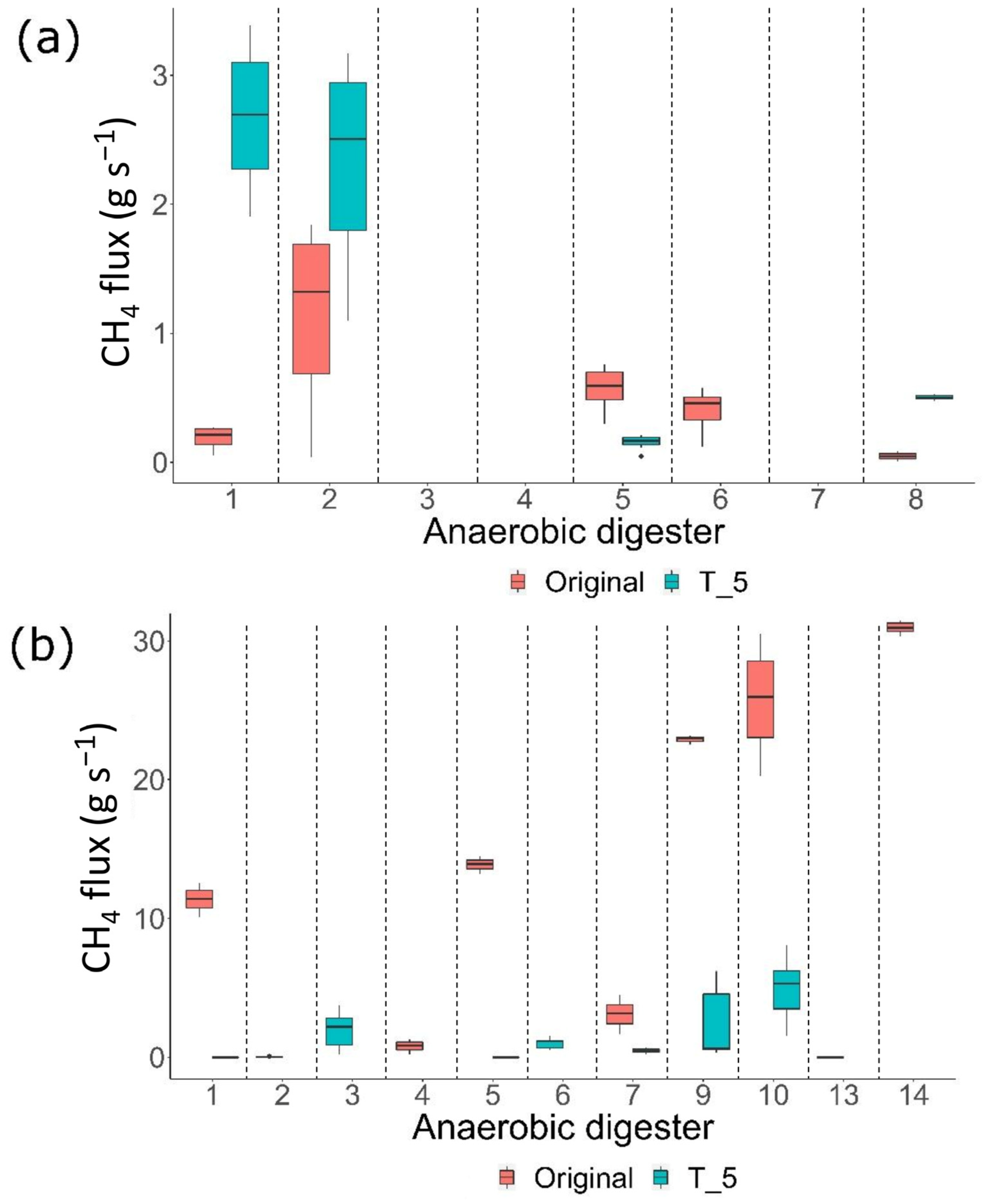
3.2.1. Anaerobic Digesters

CH₄ measurements for the flux estimation (

Table 3. CH₄ fluxes (g s⁻¹) estimated for each anaerobic digester (d) for survey 1 (21 March 2022) and survey 2 (18 May 2022) using the UAV-U10 mass balance approach. The standard deviation was calculated using the resulting flux of each set of parallel lines (a maximum of 7) used for each anaerobic digester. Only positive fluxes were considered in the calculations. The distribution of the digesters is displayed in Figure 1. BQL stands for below quantification level. T_0, T_2.5, and T_5 stand for thresholds of 0 ppm∙m, 2.5 ppm∙m, and 5 ppm∙m, respectively. “-” indicates the absence of a positive flux.

	CH4 Flux (g s−1)
	Survey 1
	Original Data Set		$\mathrm{BQL}=5\mathrm{ppm}·$m		$\mathrm{BQL}=2.5\mathrm{ppm}·$m		$\mathrm{BQL}=0\mathrm{ppm}·$m
	Original	Std. Deviation	T_5	Std. Deviation	T_2.5	Std. Deviation	T_0	Std. Deviation
d1	0.19	0.09	2.68	0.56	2.79	0.56	2.90	0.56
d2	1.14	0.67	2.32	0.79	2.35	0.77	2.43	0.78
d3	-	-	-	-	-	-	-	-
d4	-	-	-	-	-	-	-	-
d5	0.57	0.17	0.15	0.06	0.14	0.06	0.13	0.05
d6	0.40	0.16	-	-	-	-	-	-
d7	-	-	-	-	-	-	-	-
d8	0.05	0.06	0.50	0.02	0.54	0.02	0.57	0.02
Total flux	2.3 ± 0.7		5.7 ± 1.0		5.8 ± 1.0		6.0 ± 1.0
	Survey 2
	Original Data Set		$\mathrm{BQL}=5\mathrm{ppm}·$m		$\mathrm{BQL}=2.5\mathrm{ppm}·$m		$\mathrm{BQL}=0\mathrm{ppm}·$m
	Original	Std. Deviation	T_5	Std. Deviation	T_2.5	Std. Deviation	T_0	Std. Deviation
d1	11.4	0.9	0.00002	0.00002	0.00002	0.00002	0.00002	0.00002
d2	-	-	0.02	0.03	0.03	0.03	0.03	0.04
d3	-	-	1.93	1.30	2.04	1.36	2.13	1.40
d4	0.8	0.4	-	-	-	-	-	-
d5	13.9	0.5	0.0009	0.0008	0.0009	0.0008	0.0009	0.0008
d6	-	-	0.99	0.38	1.07	0.39	1.14	0.40
d7	3.1	1.0	0.47	0.19	0.48	0.20	0.51	0.21
d9	22.9	0.2	2.49	2.69	2.52	2.69	2.57	2.70
d10	25.7	3.8	4.91	2.48	4.91	2.48	4.97	2.51
d13	-	-	0.0008	0.0005	0.0008	0.0005	0.0008	0.0006
d14	31.0	0.4	-	-	-	-	-	-
Total flux	109 ± 4		11 ± 4		11 ± 4		11 ± 4

and

Table 4. CH₄ fluxes (g s⁻¹) estimated for the selected digestate storage tank using the UAV-U10 mass balance approach. Original: Original data set. T_5: Modified data set with measurements below quantification level (BQL) assumed to be 5 ppm∙m. T_2.5: Modified data set with measurements BQL assumed to be 2.5 ppm∙m. T_0: Modified data set with measurements BQL assumed to be 0 ppm∙m. The standard deviation was calculated using the resulting flux of each set of parallel lines (a maximum of 7) used for each anaerobic digester. Only positive fluxes were considered in the calculations. “-” indicates absence of a positive flux.

	(g s−1)
	CH4 Flux	Std. Deviation
Original	2.0	1.5
T_5	1.8	-
T_2.5	0.9	-
T_0	1.1	-

) were extracted from Kriging interpolations obtained for the anaerobic digesters for each of the two surveys conducted as presented in Abeywickrama et al. [19].

For survey 1, mean fluxes (Table 3) ranged from 0.05 ± 0.06 g s⁻¹ (digester 8) to 1.1 ± 0.7 g s⁻¹ (digester 2) for the original data, while total emissions for all eight digesters combined was calculated as 2.3 ± 0.7 g s⁻¹ (

Table 5. CH₄ emission estimated based on the UAV-U10 mass balance approach and the CAW method as a total flux (g s⁻¹) for each survey and an emission factor (kg CH₄ tDS⁻¹). Original: original data set. T_5: modified data set with measurements below quantification level (BQL) assumed to be 5 ppm∙m. T_2.5: modified data set with measurements BQL assumed to be 2.5 ppm∙m. T_0: modified data set with measurements BQL assumed to be 0 ppm∙m. CAW stands for carbon accounting workbook. AD and DST stand for anaerobic digester and digestate storage tanks. N denotes the number of anaerobic digesters or digestate storage tanks surveyed. The uncertainty in fluxes and emission factors is the result of propagating the standard deviations reported in Table 3 through all calculations.

Asset	Date of Survey	CH4 Flux (g s−1)						CH4 Emission Factor (kg CH4 tDS−1)
		N	Original	T_5	T_2.5	T_0	CAW	Original	T_5	T_2.5	T_0	CAW
AD	21 March 2022	8	2.3 ± 0.7	5.7 ± 1.0	5.8 ± 1.0	6.0 ± 1.0	10.22	1.9 ± 1.0	4.7 ± 3.0	4.8 ± 3.0	5.0 ± 3.2	8.4
	18 May 2022	11	109 ± 4	11 ± 4	11 ± 4	11 ± 4	14.06	65.1 ± 22.7	6.6 ± 3.3	6.6 ± 3.3	6.6 ± 3.3	8.4
DST	4 November 2022	1	2.0 ± 1.5	1.8	0.9	1.1	0.27	15.0 ± 9.9	13.5	6.8	8.3	2

). Mean fluxes for T_5 ranged from 0.15 ± 0.06 g s⁻¹ (digester 5) to 2.7 ± 0.6 g s⁻¹ (digester 1), while the total emissions for the eight digesters was 5.7 ± 1.0 g s⁻¹. Positive fluxes were not obtained for digesters 3, 4, and 7 for either the original or T_5 data sets. Only the original data set resulted in a positive flux for digester 6 (0.4 ± 0.2 g s⁻¹) (Figure 6).

For survey 2, mean fluxes (Table 3) ranged from 0.8 ± 0.4 g s⁻¹ (digester 4) to 31.0 ± 0.4 g s⁻¹ (digester 14) for the original case, while the total emissions for the 11 digesters surveyed were 109 ± 4 g s⁻¹ (Table 5). Mean fluxes for T_5 ranged from (2 ± 2) × 10⁻⁵ g s⁻¹ (digester 1) to 5 ± 2 g s⁻¹ (digester 10), while total emissions for the 11 digesters were 11 ± 4 g s⁻¹. Positive fluxes were obtained for five digesters (1, 5, 7, 9 and 10) for both the original data set and T_5. Only the original data set yielded positive fluxes for digesters 4 and 14, while T_5 yielded positive fluxes for digesters 2, 3, 6, and 13 (Table 3 and Figure 6). A tenfold difference could be observed between the total emissions estimated for the original and T_5 configurations below quantification level.

The ratios of mean fluxes between each below-quantification-level configuration (T_5, T_2.5, and T_0) were approximately 1 for all mean fluxes estimated in both surveys. Therefore, the magnitude of the differences between mean fluxes for T_5, T_2.5, and T_0 can be considered negligible. However, there was a significant difference between the mean fluxes of the original and all below-quantification-level configurations.

3.2.2. Digestate Storage Tanks

Similar to the anaerobic digesters, CH₄ measurements were extracted from the Kriging interpolations obtained for different cases (original, T_5, T_2.5, T_0), as presented in Abeywickrama et al. [19].

The maximum mean flux estimated for the original case during survey 3 was 2.0 ± 1.5 g s⁻¹, while it was the minimum for T_2.5 at ≈0.9 g s⁻¹ (Table 4). The standard deviations for T_5, T_2.5, and T_0 could not be calculated as only one flux was positive for T_5, T_2.5, and T_0 among the seven estimated fluxes (Table 4). This reflects the variability of the CH₄ plume close to the tank at 1 m intervals.

3.3. CH₄ Fluxes Estimated by the Carbon Accounting Workbook (CAW)

3.3.1. Anaerobic Digesters

The equivalent total CH₄ emission estimated with the CAW for the fourteen anaerobic digesters which were operational was 17.89 g s⁻¹. Therefore, the average emission estimation per anaerobic digester was 1.28 g s⁻¹.

For survey 1, the CAW equivalent flux for the eight digesters surveyed was 10.22 g s⁻¹. The CAW estimation was higher than those obtained with the mass balance approach (Table 5). The CAW flux estimation was approximately 4 times higher than the original case (2.3 ± 0.7 g s⁻¹) and 1.7 times higher than any of the remaining cases.

For survey 2, the eleven digesters surveyed according to the CAW were 14.06 g s⁻¹ (Table 5). The flux estimated with the mass balance approach for the original data set was approximately 8 times higher than that obtained for the CAW estimation, while T_5, T_2.5 and T_0 estimations were approximately 0.8 times lower (11 ± 4 g s⁻¹).

3.3.2. Digestate Storage Tanks

The total CH₄ emission was 4.26 g s⁻¹ for the sixteen digestate storage tanks based on the CAW. The CAW equivalent average flux per tank was 0.27 g s⁻¹. The estimations based on the mass balance approach were approximately 7, 7, 3, and 4 times greater than the CAW estimations for the original, T_5, T_2.5, and T_0 data sets, respectively (Table 5).

4. Discussion

This paper focuses on the quantification of CH₄ emissions from both open and closed sludge treatment assets. It compares the emission rates obtained by surveying full-scale assets with a UAV-U10, and using the mass balance approach, with emissions estimated according to the carbon accounting workbook (CAW), which is the tool of choice of the UK water industry. The study shows that the CAW provides significantly reduced emission estimates when compared to the UAV-U10 approach for open assets on the study site. The largest differences between estimated emissions from both methods was observed for anaerobic digesters (survey 2—original data set vs. CAW) and reached a magnitude of approximately 95 g s⁻¹ (57 kg CH₄ tDS⁻¹), which is almost eightfold higher than the CAW estimates. For the digestate storage tanks, the UAV-U10 fluxes were up to nearly an order of magnitude (approx. 1.7 g s⁻¹ (13 kg CH₄ tDS⁻¹)) higher than the CAW estimates for some of the below-quantification-level configurations (original and T_5). This study also exhibits that emission estimations for the two assets considered were substantially different.

Overall, the anaerobic digesters for survey 2 (original data set) showed a significant contribution to the CH₄ emissions (≈10 g s⁻¹ per digester). However, it is important to note that a lower number of CH₄ concentration measurements above the level of quantification was obtained for survey 2 (284 points) than for survey 1 (3771 points). This discrepancy of 3487 points between surveys could explain some of the differences in estimated emissions. However, the number of concentration readings obtained during survey 2 was significantly larger than what would have been obtained with more traditional methods (e.g., handheld sensor) and provides better spatial coverage than static ground sensors.

The maximum recorded emission rate during survey 1 was approx. 0.75 g s⁻¹ per digester or 5 kg CH₄ tDS⁻¹. During survey 3, emissions from digestate storage tanks were approximately 2.0 g s⁻¹ per tank or 15 kg CH₄ tDS⁻¹, underlining their notable sensitivity on the overall emission. While site measurements and the mass balance approach suggested higher CH₄ emissions from digestate storage tanks, the variability of the measurements obtained did not enable us to determine whether these differences were statistically significant.

The results of this cross-asset comparison were not consistent with those by UKWIR [8] (CAW), which identifies anaerobic digesters as the major contributor across both assets, while site results emphasize the strong contribution of digestate open storage towards site-level emissions. This relative contribution varies greatly according to site asset management practices, which influence the repair frequency for leaks of closed anaerobic digesters.

Daelman et al. [12] reported an emission estimation for digestate storage tanks of 4 kg CH₄ h⁻¹ (≈1 g s⁻¹), which, overall, is lower than the estimates from this study obtained with the combined UAV-U10 mass balance approach. Differences between fluxes estimated with each approach could be due to a wide range of factors. There are assumptions and inaccuracies associated with the mass balance approach that could compromise fluxes estimated with the UAV-U10 approach. For example, the mass balance approach assumes stable wind conditions during data collection and CH₄ flowing into and out from the specified box volume only through upwind and downwind surfaces. Allen et al. [17] recommended that downwind measurements be taken at least 100–300 m apart compared to the width of their surveyed area when applying the mass balance approach to quantify landfill CH₄ emissions. In the present study, fluxes were estimated based on CH₄ concentrations measured within a few meters (2–10 m) from the source due to the distribution of the assets within the WWTP. Yang et al. [24] tested the mass balance approach with close-to-source monitoring against controlled releases of CH₄. They observed that 30% of the total tests could estimate fluxes with percentage errors < 20%, and out of those, 70% of the tests occurred when there were steady wind speeds of approximately 3–6 m s⁻¹. They stated that the CH₄ estimations were also highly sensitive to GPS noise of 1–2 m. The UAV platform used in this study has an accuracy up to 1 cm + 1 ppm in planimetry and 1.5 cm + 1 ppm in altimetry, and the average wind speed during the surveys was between ≈2.8–5.8 m s⁻¹. Based on these results, the GPS noise of the UAV platform used in this study can be considered negligible, and the wind speed during the surveys can be considered stable.

The mass balance approach presented here uses Kriging geostatistical techniques to interpolate the data collected with the UAV-U10. Deterministic interpolation methods, such as inverse distance weighted interpolation, were not considered suitable because they do not utilize the statistical properties of the measured CH₄ points. Kriging provides a measure of certainty for the interpolation by considering the spatial arrangement of the data, making it more suitable for data sets with directional bias, such as those influenced by wind speed and direction. However, there may be an impact on the flux calculation due to using points spaced at 3.2 cm intervals while the actual measurements are spaced every 2 m or more. Although uncertainties can arise from using Kriging for interpolated values, this interpolation was necessary to generate a data set large enough to confidently implement Simpson’s rule integration.

For flux estimation, it is essential for the wind component to be measured accurately as it plays a major role in the mass balance approach. Shaw et al. [25] described that it would be preferable for the wind component to be measured on-board of the UAV, with the measuring frequency matching or exceeding that of the CH₄ measurement for accurate flux estimations. In the study presented here, the wind component was measured on-board the UAV, but the records were not temporally collocated with those for CH₄. The frequency of CH₄ measurements depended on the CH₄ detection capability, with the time interval between two measurements being on the order of milliseconds. The frequency of wind measurements ranged from 5 to 15 s. This lack of temporally collocated measurements could have influenced the accuracy of the flux estimation. The reflective characteristics of the ground surface had a significant influence on the observed U10 vertical path integrated CH₄ concentrations. According to AiLF [22], the test conditions for the minimum detection limit of the U10 (5 ppm∙m) were 20 m to a reflective gypsum surface. The total number of measurements below quantification level could have varied depending on the distance to and the roughness of the reflective surface. This, in turn, would have eventually influenced the estimated fluxes. Therefore, there is a need to quantify the sensitivity of the framework presented here using experimental set ups in a controlled environment.

Similarly, the way the U10 below quantification level was determined could also have had an impact on the final flux calculations. The below-quantification-level effect was significant enough to shift flux estimations from positive to negative for some of the assets. There is also the added factor of substantial spatial and temporal variation in emissions in open assets, in addition to the effect of near-field turbulences and interference from adjacent sources, such as secondary roads and motorways. For example, near-field turbulences can trigger sub-meter flux variations. The close proximity of WWTP assets was also expected to have an influence on the accuracy of the flux estimations.

With regard to CAW estimations, total sludge inflow could have varied due to different sludge volumes being produced on the wastewater treatment line or the variability of the imports received from satellite sites, ultimately introducing uncertainty to the calculated average digester feed. The CAW also assumes a constant emission factor throughout the year, neglecting the dynamic profile of emissions linked to differences in treatment volumes, variable operational conditions, and changes in environmental conditions. To illustrate this, Maldaner et al. [23] evidenced a 12-fold increase in residual CH₄ emissions in July compared to April, coinciding with a 3-fold increase in digestate temperature. The authors stated that temperature alone cannot be a CH₄ emission predictor, as incoming sludge composition, digestate storage depth, and changing retention time could also influence emission potential. Daelman et al. [12] also evidenced an inverse proportionality between anaerobic digester residence time and CH₄ emissions from digestate storage tanks. Moore et al. [29] also supported that CH₄ emissions from WWTPs, particularly those with anaerobic digesters, are underestimated by current IPCC-based estimates. They emphasised that additional data from plant operators, including treatment processes and daily loading, can help create informed emission factors. One significant advantage of UAV measurements is that once the UAV survey is planned, it is capable of quantifying numerous assets under various conditions. This allows for the exploration of primary sources of variability while complementing data on both operational and environmental conditions.

CH₄ can be emitted from digestate to the atmosphere even after anaerobic digestion has taken place, either by releasing dissolved CH₄ due to turbulence caused by mixing and pumping or as a result of the continuation of the digestion process by active methanogenic archaea [8]. Previous authors [23] have reported CH₄ emissions of 1.0 kg m⁻³ yr⁻¹ (~0.1 g CH₄ m⁻³ h⁻¹) from digestate storage at a dairy manure biogas facility after anaerobic digestion took place. Fredenslund et al. [30] reported that 53% of the total CH₄ emissions from a biogas plant treating sludge from a WWTP, equivalent to approx. 3.4 kg CH₄ h⁻¹, originated from digestate storage tanks with a 12 h retention time. However, this estimation assumed that CH₄ formation in the digestate storage tank would be the same as CH₄ formation in digesters (∼6.7 g CH₄ m⁻³ h⁻¹). In reality, the CH₄ emission rate can be influenced by ambient conditions and the cooling of the digestate. For the digestate storage tank surveyed in this study, the digestate was fresh and at a higher temperature than any of the other tanks. Emissions from this tank were expected to be larger than adjacent tanks, which contained aged digestate covered by a crust. Freshness and temperature were variable across tanks and along the sludge retention time due to exposure to ambient air temperature [16]. This is consistent with the results obtained by Maldaner et al. [23]. The authors observed that there was a correlation between digestate temperature and CH₄ emissions. Further work should focus on identifying the sludge retention cycle of each digestate storage tank and associated temperatures to model the expected emission at each stage of the process, considering that temperature can impact not only emissions, but also the rate of emissions, which makes profiling of emissions dynamics critical.

The CAW assumes that all advanced anaerobic digesters are newly built and, thus, associated with minimized fugitive emissions. This assumption is, in fact, a significant limitation, as it is not factually correct in some instances. For example, at Minworth, thermal pre-treatment was retrofitted to preexisting anaerobic digesters without renovating them. Therefore, neither emission estimates based on emission factors for conventional anaerobic digesters nor refurbished advanced anaerobic digesters were representative of the actual emissions. The CAW also assumes that digestate storage tank emissions comprise one-fourth of the emissions attributed to full secondary open digesters. This is based on a linear reduction in CH₄ emission potential from digestate with retention time that oversimplifies the dynamics of emissions.

These results evidence that emission estimation based on a single emission factor and total annual sludge inflow do not account for the variability of emissions. There is a need to revise current common reporting practices through the inclusion of environmental and operational factors. Further research should focus on validation of the UAV-U10 approach and below-quantification-level data handling in a controlled environment, with controlled release of CH₄.

Emissions estimation in WWTPs is generally carried out at the plant level [8] or for leak detection [18,24]. Further work on the estimation of asset-specific fluxes is required in order to effectively manage emissions and prioritise intervention strategies for abatement. The work presented here contributes to addressing this challenge by applying the mass balance approach for CH₄ flux estimation to separate assets. From an emission management perspective, it is recommended to focus on enhancing the base knowledge of process emissions from open assets (e.g., digestate storage tanks) to achieve net zero targets. Emissions from closed assets could be substantially minimised by repair and maintenance. Bespoke solutions could also be designed to more effectively control emissions.

This study has highlighted how emission estimations can differ depending upon the method used. It has also been reported that there are both temporal (as per results shown in study by Abeywickrama et al. [19] and Maldaner et al. [23]) and spatial variabilities (such as digestate storage tanks being in different stages of CH₄ emission levels) that need to be taken into account when estimating fluxes. These lead to the requirement of CH₄ flux estimation to be based on on-site CH₄ measurements and monitoring techniques.

When it comes to on-site measurements, UAVs seem to be a cost-effective solution; collecting a similar number of measurements with ground sensors requires multiple sensors at different altitudes, as well as increased sensor deployment and maintenance. UAVs also provide de-risked operations, as direct access to the emission source is not required. However, it is important to note that the feasibility of using UAVs for on-site measurements will have to be assessed for a wider range of environmental conditions than the one captured by the work presented here. The UAV-U10 monitoring framework presented here could be employed to replicate the estimation of emissions across multiple surveys conducted under different environmental conditions and operational scenarios. Further work should look at specifying the frequency required to capture temporal variability in emission fluxes per asset, determining asset-specific sampling densities, and reaching a consensus on how the values below quantification level and the permissible emission uncertainty levels should be treated.

Survey replicability will have to take into account future technological developments. For example, a rapid switch to much higher-precision instruments are expected in the next few years, with sensors providing precision levels of up to 0.9 ppb. The ABB system with cavity ringdown spectroscopy that was mounted on-board a DJI M600 UAV by Yong et al. [31] is perhaps the first use of such technology and demonstrates the feasibility of the sensor integration. Note that the increased weight of more precise sensors (ABB 2.5 kg vs. U10 0.52 kg) could curtail the integration of the sensor on small UAV platforms and limit the uptake of the technology.

This study provides a set of flux estimation guidelines transferable to different WWTPs and industrial sectors. The transferability of the framework at this stage is restricted to study areas with suitable monitoring conditions for the deployment of the UAV platform and the collection of data with the U10 sensor. The UAV-U10 framework is suitable for the quantification of area sources for which the location of the emission is known. In contrast, point source emissions, such as leaks, would be more challenging to monitor, as the UAV-U10 would not be able to identify the exact location of the source. Nonetheless, the framework would always be useful for the provision of emission estimations.

The UAV-U10 framework could contribute to the development of atmospheric measurement standards and targets as required by the Office for Environment Protection. Further, standardizing emission estimation across all sectors will result in a more straightforward comparison of emissions across sectors and increased pace towards achieving net zero targets [4].

5. Conclusions

This manuscript presents a framework to convert vertical path-integrated CH₄ concentrations collected through UAV-U10 for sludge treatment centres to asset-level mass fluxes. The approach proposed for flux calculation is a step forward from the current common reporting practice (CAW). It was concluded that UAV monitoring coupled with the mass balance approach is cost-effective compared to tracer transport modelling techniques and might be a more realistic representation of the actual emissions. The UAV monitoring framework could be utilized to repeat surveys and assist in modelling expected emissions at different process stages.

The results highlight that different assets present different emission levels. Overall, anaerobic digesters present higher CH₄ emissions than digestate storage tanks. However, these results heavily depend on specific maintenance and repair works at each site. Similarly, the results also showed substantial differences between CAW and UAV-U10 flux estimates within and between assets. Overall, for the anaerobic digesters, the UAV-U10 framework showed reduced fluxes when compared to CAW estimates, except for some digesters, where the UAV-U10 estimation was an order of magnitude larger than the CAW estimate. Flux estimates for the digestate storage tanks seem to be underreported in all instances when using CAW. The results suggest that priority should be given to developing better monitoring strategies for CH₄ emissions, especially focusing on digestate storage tanks.

The mass balance approach presented here provides asset-specific emission estimations (e.g., digester level), whereas the current CAW method is not capable of providing estimates at such a fine resolution. It also allows water utilities to make more targeted and better-informed management decisions, such as prioritising specific anaerobic digesters for maintenance. Capturing spatial and temporal variations, which are essential, especially for open assets, can be achieved through planning the flux estimation frequency as recommended by Abeywickrama et al. [19] for both anaerobic digesters and digestate storage tanks.

References

1. Rogelj, J.; den Elzen, M.; Höhne, N.; Fransen, T.; Fekete, H.; Winkler, H.; Schaeffer, R.; Sha, F.; Riahi, K.; Meinshausen, M. Paris Agreement climate proposals need a boost to keep warming well below 2 °C. Nature 2016, 534, 631–639. [Google Scholar] [CrossRef] [PubMed]
2. Water UK; Ricardo; MacDonald, M. Net Zero 2030 Routemap. 2020. Available online: https://www.water.org.uk/sites/default/files/2023-08/Water-UK-Net-Zero-2030-Routemap.pdf (accessed on 19 May 2024).
3. Forster, P.; Storelvmo, T.; Armour, K.; Collins, W.; Dufresne, J.L.; Frame, D.; Lunt, D.J.; Mauritsen, T.; Palmer, M.D.; Watanabe, M.; et al. Chapter 7: The Earth’s Energy Budget, Climate Feedbacks, and Climate Sensitivity. In IPCC Sixth Assessment Report; Cambridge University Press: Cambridge, UK; Cambridge University Press: New York, NY, USA, 2021; pp. 923–1054. [Google Scholar] [CrossRef]
4. Skea, J.; Shukla, P.; Reisinger, A.; Slade, R.; Pathak, M.; Khourdajie, A.; Diemen, R.; Abdulla, A.; Akimoto, K.; Babiker, M.; et al. Climate Change 2022, Mitigation of Climate Change Summary for Policymakers (SPM). 2022. Available online: https://www.ipcc.ch/report/ar6/wg2/ (accessed on 19 May 2024).
5. Doorn, M.R.J.; Towprayoon, S.; Vieira, S.; Irving, W.; Palmer, C.; Pipatti, R.; Wang, C. Chapter 6 Wastewater Treatment and Discharge. In 2006 IPCC Guidelines for National Greenhouse Gas Inventories Volume 5 Waste; Intergovernmental Panel On Climate Change: Geneva, Switzerland, 2006; Volume 5, pp. 1–56. [Google Scholar]
6. Hill, N.; Karagiani, E.; Jones, L.; MacCarthy, J.; Bonifazi, E.; Hinton, S.; Walkr, C.; Harris, B. 2021 Government Greenhouse Gas Conversion Factors for Company Reporting: Methodology Paper; Department for Business Energy & Industrial Strategy (BEIS): London, UK, 2021. Available online: https://assets.publishing.service.gov.uk/government/uploads/system/uploads/attachment_data/file/904215/2019-ghg-conversion-factors-methodology-v01-02.pdf (accessed on 19 May 2024).
7. Kuylenstierna, J.C.; Michalopoulou, E.; Malley, C. Global Methane Assessment Benefits and Costs of Mitigating Methane Emissions; Climate & Clean Air Coalition & UN Environment Programme: Paris, France, 2021. [Google Scholar]
8. Brotto, A.; Kraakman, B.; Kyne, C.; Lake, A.; Perez, E.R.; Scott, S. Quantifying and Reducing Direct Greenhouse Gas Emissions from Waste and Water Treatment Process—Phase 1; UK Water Industry Research: London, UK, 2020. [Google Scholar]
9. European Industrial Emissions Portal. Pollutant Index. Available online: https://industry.eea.europa.eu/pollutants/pollutant-index (accessed on 18 May 2024).
10. Delre, A.; Mønster, J.; Scheutz, C. Greenhouse gas emission quantification from wastewater treatment plants, using a tracer gas dispersion method. Sci. Total Environ. 2017, 605–606, 258–268. [Google Scholar] [CrossRef] [PubMed]
11. Aboobakar, A. Quantification of Greenhouse Gas Emissions in Biological Wastewater Treatment. Ph.D. Thesis, Cranfield University, Cranfield, UK, 2014. [Google Scholar]
12. Daelman, M.R.J.; van Voorthuizen, E.M.; van Dongen, U.G.J.M.; Volcke, E.I.P.; van Loosdrecht, M.C.M. Methane emission during municipal wastewater treatment. Water Res. 2012, 46, 3657–3670. [Google Scholar] [CrossRef] [PubMed]
13. Doorn, M.R.J.; Strait, R.P.; Barnard, W.R.; Pechan, E.H.; Eklund, B.; Thorneloe, S.A. Estimates of Global Greenhouse Gas Emissions from Industrial and Domestic Wastewater Treatment; US EPA Office of Research and Development, Air Pollution Prevention and Control Division: Research Triangle Park, NC, USA, 1997. [Google Scholar]
14. Kosse, P.; Knoop, O.; Lübken, M.; Schmidt, T.C.; Wichern, M.; Methane Emissions from Wastewater Treatment Plants-Assessment and Review of Quantification Methods. WaterSolutions, International Energy Agency Bioenergy 2018. Available online: https://www.researchgate.net/publication/323308510 (accessed on 19 May 2024).
15. Parravicini, V.; Svardal, K.; Krampe, J. Greenhouse Gas Emissions from Wastewater Treatment Plants. In Energy Procedia; Elsevier Ltd.: Amsterdam, The Netherlands, 2016; pp. 246–253. [Google Scholar] [CrossRef]
16. Liebetrau, J.; Reinelt, T.; Agostini, A.; Linke, B. Methane Emissions from Biogas Plants; International Energy Agency Bioenergy: Paris, France, 2017; Available online: https://www.ieabioenergy.com/wp-content/uploads/2018/01/Methane-Emission_web_end_small.pdf (accessed on 19 May 2024).
17. Allen, G.; Pitt, J.; Hollingsworth, P.; Mead, I.; Kabbabe, K.; Roberts, G.; Percival, C. Measuring Landfill Methane Emissions Using Unmanned Aerial Systems: Field Trial and Operational Guidance. 2015. Available online: https://www.gov.uk/government/publications/measuring-landfill-methane-emissions-using-unmanned-aerial-systems (accessed on 19 May 2024).
18. Nathan, B.J.; Golston, L.M.; O’brien, A.S.; Ross, K.; Harrison, W.A.; Tao, L.; Lary, D.J.; Johnson, D.R.; Covington, A.N.; Clark, N.N.; et al. Near-Field Characterization of Methane Emission Variability from a Compressor Station Using a Model Aircraft. Environ. Sci. Technol. 2015, 49, 7896–7903. [Google Scholar] [CrossRef] [PubMed]
19. Abeywickrama, H.G.K.; Bajón-Fernández, Y.; Srinamasivayam, B.; Turner, D.; Casado, M.R. Development of a UAV Based Framework for CH4 Monitoring in Sludge Treatment Centres. Remote Sens. 2023, 15, 3704. [Google Scholar] [CrossRef]
20. Shorrock, C.; Driessen, W.; Snelson, P.; Chadha, M. Advanced Reject Water Treatment. 2014. Available online: https://waterprojectsonline.com/wp-content/uploads/case_studies/2012/Minworth-STW-Anammox-Plant-2012.pdf (accessed on 19 May 2024).
21. Esri. ‘Imagery’ [basemap]. Scale Not Given. ‘World Imagery’. 12 December 2009. Available online: https://www.arcgis.com/home/item.html?id=10df2279f9684e4a9f6a7f08febac2a9 (accessed on 19 May 2024).
22. AiLF. User Manual UAV Based Laser Methane Leakage Detector; AiLF (Shandong) Instruments Inc.: Jinan, China, 2019; Available online: https://www.manualslib.com/manual/1860232/Ailf-U10.html (accessed on 19 May 2024).
23. Maldaner, L.; Wagner-Riddle, C.; VanderZaag, A.C.; Gordon, R.; Duke, C. Methane emissions from storage of digestate at a dairy manure biogas facility. Agric. For. Meteorol. 2018, 258, 96–107. [Google Scholar] [CrossRef]
24. Yang, S.; Talbot, R.W.; Frish, M.B.; Golston, L.M.; Aubut, N.F.; Zondlo, M.A.; Gretencord, C.; McSpiritt, J. Natural gas fugitive leak detection using an unmanned aerial vehicle: Measurement system description and mass balance approach. Atmosphere 2018, 9, 383. [Google Scholar] [CrossRef]
25. Shaw, J.T.; Shah, A.; Yong, H.; Allen, G. Methods for quantifying methane emissions using unmanned aerial vehicles: A review. Philos. Trans. R. Soc. A Math. Phys. Eng. Sci. 2021, 379, 20200450. [Google Scholar] [CrossRef] [PubMed]
26. Shah, A.; Allen, G.; Pitt, J.R.; Ricketts, H.; Williams, P.I.; Helmore, J.; Finlayson, A.; Robinson, R.; Kabbabe, K.; Hollingsworth, P.; et al. A near-field Gaussian plume inversion flux quantification method, applied to unmanned aerial vehicle sampling. Atmosphere 2019, 10, 396. [Google Scholar] [CrossRef]
27. Yamartino, R.J. A Comparison of Several ‘Single-Pass’ Estimators of the Standard Deviation of Wind Direction. Clim. Appl. Meteorol. 1984, 23, 1362–1366. [Google Scholar]
28. Allen, G.; Hollingsworth, P.; Kabbabe, K.; Pitt, J.R.; Mead, M.I.; Illingworth, S.; Roberts, G.; Bourn, M.; Shallcross, D.E.; Percival, C.J. The development and trial of an unmanned aerial system for the measurement of methane flux from landfill and greenhouse gas emission hotspots. Waste Manag. 2019, 87, 883–892. [Google Scholar] [CrossRef] [PubMed]
29. Moore, D.P.; Li, N.P.; Wendt, L.P.; Castañeda, S.R.; Falinski, M.M.; Zhu, J.-J.; Song, C.; Ren, Z.J.; Zondlo, M.A. Underestimation of Sector-Wide Methane Emissions from United States Wastewater Treatment. Environ. Sci. Technol. 2023, 57, 4082–4090. [Google Scholar] [CrossRef] [PubMed]
30. Fredenslund, A.M.; Hinge, J.; Holmgren, M.A.; Rasmussen, S.G.; Scheutz, C. On-site and ground-based remote sensing measurements of methane emissions from four biogas plants: A comparison study. Bioresour. Technol. 2018, 270, 88–95. [Google Scholar] [CrossRef] [PubMed]
31. Yong, H.; Allen, G.; Mcquilkin, J.; Ricketts, H.; Shaw, J.T. Lessons learned from a UAV survey and methane emissions calculation at a UK landfill. Waste Manag. 2024, 180, 47–54. [Google Scholar] [CrossRef] [PubMed]
Figure 1. Asset distribution at Minworth wastewater treatment plant, generated using ArcGIS Pro 2.8. Source: [21]. The red polygon shows the anaerobic digesters. The blue polygon determines the extent of the digestate storage tanks. The numbers denote individual units within the asset. The yellow lines indicate individual digestate storage tanks. The numbers on the axes of the image represent GIS coordinates (latitude and longitude, World Geodetic System 1984 (WGS84)). These coordinates are measured in meters relative to a reference point on the Earth’s surface.
Remotesensing 16 02280 g001
Figure 2. Images of the sensors and the UAV platform used for data collection. (a) Matrice 300 RTK DJI UAV equipped with the U10 sensor (DJI, China). (b) DJI Zenmuse H20T thermal sensor. (c) Thermal imagery showing the difference in temperature between the surveyed digestate storage tank (left) and an adjacent tank (right) within the asset; cold areas are depicted in blue while warm areas are depicted in yellow.
Remotesensing 16 02280 g002
Figure 3. Workflow of data collection and analysis. (a) Overall workflow of data collection and process. (b) Workflow of flux estimation based on the mass balance approach and the spatial distribution of anaerobic digesters. Source: [21] (c) Workflow for the CAW approach. ([CH4]–[CH4]b) are the path integrated concentrations in ppm∙m, u ¯ is the mean wind speed (m s−1) perpendicular to the vertical plane of which the plume is projected, and dx is infinitesimal differences (m) along the horizontal direction in the plane perpendicular to the wind speed u ¯ . AD, DST, EF, and CAW stand for anaerobic digester, digestate storage tank, emission factor, and carbon accounting workbook, respectively.
Remotesensing 16 02280 g003
Figure 4. Illustration of the pairs of parallel lines used to determine upwind and downwind measurements for the anaerobic digesters (a) and the digestate storage tank (b).
Remotesensing 16 02280 g004
Figure 5. CH4 point measurements collected during each survey: (a) survey 1—anaerobic digesters surveyed on 21 March 22; (b) survey 2—anaerobic digesters surveyed on 18 May 22; and (c) survey 3—digestate storage tank surveyed on 4 November 22.
Remotesensing 16 02280 g005
Figure 6. Box plots of estimated CH4 fluxes for each anaerobic digester. Original: original data set. T_5: Modified data set with measurements below quantification level (BQL) assumed to be 5 ppm∙m. The box represents the interquartile range. (a) Data set collected on 21 March 2022. (b) Data set collected on 18 May 2022.
Remotesensing 16 02280 g006