Abstract
Remote images are useful tools for detecting and monitoring landslides, including shallow landslides in agricultural environments. However, the use of non-commercial satellite images to detect the latter is limited because their spatial resolution is often comparable to or greater than landslide sizes, and the spectral characteristics of the pixels within the landslide body (LPs) are often comparable to those of the surrounding pixels (SPs). The buried archaeological remains are also often characterized by sizes that are comparable to image spatial resolutions and the spectral characteristics of the pixels overlying them (OBARPs) are often comparable to those of the pixels surrounding them (SBARPs). Despite these limitations, satellite images have been used successfully to detect many buried archaeological remains since the late 19th century. In this research context, some methodologies, which examined the values of OBARPs and SBARPs, were developed to rank images according to their capability to detect them. Based on these previous works, this paper presents an updated methodology to detect shallow landslides in agricultural environments. Sentinel-2 and Google Earth (GE) images were utilized to test and validate the methodology. The landslides were mapped using GE images acquired simultaneously or nearly simultaneously with the Sentinel-2 data. A total of 52 reference data were identified by monitoring 14 landslides over time. Since remote sensing indices are widely used to detect landslides, 20 indices were retrieved from Sentinel-2 images to evaluate their capability to detect shallow landslides. The frequency distributions of LPs and SPs were examined, and their differences were evaluated. The results demonstrated that each index could detect shallow landslides with sizes comparable to or smaller than the spatial resolution of Sentinel-2 data. However, the overall accuracy values of the indices varied from 1 to 0.56 and two indices (SAVI and RDVI) achieved overall accuracy values equal to 1. Therefore, to effectively distinguish areas where shallow landslides are present from those where they are absent, it is recommended to apply the methodology to many image processing products. In conclusion, given the significant impact of these landslides on agricultural activity and surrounding infrastructures, this methodology provides a valuable tool for detecting and monitoring landslide presence in such environments.
1. Introduction
Shallow landslides significantly contribute to soil erosion, especially in agricultural areas, where their frequency and impact have increased due to extreme weather events [1]. Over recent decades, mapping these phenomena has become crucial in the context of climate change, leading to extensive efforts to map shallow landslides using satellite imagery [2,3,4]. Researchers have utilized optical satellite images to develop algorithms for the rapid and (semi-)automated detection of landslides after triggering events [5,6]. Recently, experiments have employed Synthetic Aperture Radar (SAR) images [7,8] although detecting and mapping landslides using SAR remains challenging [9]. Additionally, numerous studies in agricultural areas have employed an Unmanned Aerial Vehicle (UAV) [10,11,12,13].
Several researchers have assessed slope instability by examining vegetation characteristics [14,15]. They have investigated how geomorphological processes on hillslopes create anomalies in vegetation by analyzing vegetation indices alongside morphometric features [14,15]. For instance, a recent study identified vegetation changes and correlated these spatial–temporal variations with landslide creep induced by an earthquake [16]. Image processing products such as the normalized differential vegetation index (NDVI), spectral angle, principal component analysis (PCA), and independent component analysis (ICA) have been used to map landslides from FORMOSAT-2 satellite images [17,18]. Vegetation indices are commonly used worldwide to detect landslides by highlighting land cover changes before and after landslide events [14,16]. Some researchers have mapped landslides through visual inspection of vegetation indices [3,16] whereas others have developed semi-automated or automated methods [17]. Additionally, many studies have combined vegetation indices with morphometric characteristics derived from LIDAR or high-resolution digital terrain models (DTMs) [19].
Despite these advancements, the detection of shallow landslides in hilly agricultural areas remains underexplored due to several factors: (i) the shallow landslides involve a subtle depth of soil, and they are characterized by a short runout distance [20]. Therefore, the pixels corresponding to the landslide body do not exhibit specific spectral characteristics with respect to the pixels surrounding them; (ii) the number of pixels corresponding to shallow landslides may be limited because their size may be very small. However, the few pixels corresponding to the landslide body may have a different spectral signal from the surrounding pixels; (iii) these landslides are often intermittent with periodic reactivation due to rainfall following seasonal ploughing activities, complicating their detection over the time.
Given the challenges associated with shallow landslide detection, it is crucial to explore and test various approaches. Detecting a shallow landslide in an image hinges on the premise that the pixel values within the landslide (LPs) differ from the surrounding pixel values (SPs), even though their land cover and land use are the same. Additionally, the size of shallow landslides in agricultural environments is often smaller than the pixel size of most non-commercial satellite images. Consequently, most non-commercial satellite sensors, including Sentinel-2 sensors, can rarely detect or monitor (detect over time) their occurrence and very rarely can map them.
In summary, although remote images have been extensively used to detect, map, and monitor landslides globally [14,15], shallow landslides in agricultural settings were poorly detected and monitored using non-commercial satellite sensors. As a matter of fact, their dimensions are comparable or smaller than the spatial resolution of the satellite images, and the characteristics of LPs are comparable to those of SPs. The shallow landslides in agricultural environments share these characteristics with buried archaeological remains. In other words, the sizes of many buried archaeological remains (e.g., streets and walls) are comparable to the spatial resolutions of remote images. Moreover, the spectral features of the OBARPs are comparable to those of SBARPs. Despite these limitations, the buried archaeological remains and the shallow landslides can leave their marks on images due to their impact on soil moisture distribution and vegetation characteristics [20,21,22,23].
Since the end of the nineteen century, remote images have been used to detect buried archeological remains by exploiting the different values of OBARPs and SBARPs (e.g., [22,24]). Visual interpretation of images and/or image-processing products has been a common practice for detecting buried remains [25,26,27]. The papers noted that the capability to detect them in an image depends on many factors (e.g., the characteristics of the sensor, buried structure, soil and/or vegetation; the morphological and geologic characteristics of the study area; the conditions under which the sensor acquired the image [28,29]). Therefore, the authors highlighted that a single image or image processing product does not allow the detection of buried remains at every site and time, and they suggested evaluating many images or image processing products to enhance detection accuracy. For the latter finding, some papers proposed a method for evaluating the detection capability of images or image processing products [25,26,30]. These methods were developed to detect buried archeological remains characterized by a size comparable to or greater than the spatial resolution of remote images. The authors compared the values of pixels overlying buried structures (OBARPs) with the values of pixels not immediately adjacent to them (SBARPs) [25,26,30]. They also proposed different assessment parameters independent of the photo-interpreter’s skill that can always be refuted. For example, Cavalli et al. [26] introduced two parameters for quantifying the differences between the values of OBARPs and SBARPs, detection and separability indices. These assessment parameters allow for the analysis of multiple images or image processing products, enabling archaeologists to focus visually on the most effective images or products [26,30]. Furthermore, all these works validated the proposed methodology by comparing the identified buried archaeological remains with the reference data that were derived from other sensors [31]. For example, Cavalli et al. [26] validated the methodology using an archeological street network that “was first identified on aerophotos by Schmiedt [32] and partly confirmed by successive archaeological investigations [33,34] and by geomagnetic and geoelectric prospections [35]”.
Starting from these studies, we proposed an updated methodology from previous ones [26,30] for evaluating the ability to detect and monitor the shallow landslides in agricultural environments using an assessment parameter that was independent of the photo-interpreter’s skill. The previous methodology primarily focused on identifying buried structures that were characterized by linear geometry (i.e., streets and walls) and by sizes that are comparable to or greater than the spatial resolution of the images. In contrast to these structures, landslides exhibit irregular and non-linear geometric characteristics and have dimensions comparable to or smaller than the pixel resolution. Given these differences, the methodology has been modified to achieve the primary objective of this work: highlighting the boundaries of each landslide. To this end, the method of selecting regions of interest (ROI) was revised. In the current approach, two ROIs (LP and SP) were identified for each landslide, with SPs located adjacent to LPs. Unlike the previous archaeological approach, where the two ROIs (OBARPs and SBARPs) were not adjacent, this work ensures that the SPs were immediately adjacent to the LPs. Furthermore, a single assessment parameter was used to quantify the difference between the two ROIs, whereas the previous methodology used two parameters. The authors validated the new assessment parameter using 52 reference data addressing an important issue: can this methodology successfully detect and monitor shallow landslides characterized by a size smaller than the pixel size of the satellite images employed? For this purpose, we calculated several remote sensing indices by using Sentinel-2 images. Hence, we addressed another two important issues: is there a remote sensing index that can adequately detect shallow landslides? Does the possibility of detecting landslides increase with the number of indices calculated? The proposed methodology, and remote and reference data are described in Section 2, whereas the results, discussion, and conclusions are presented in Section 3 and Section 4, respectively.
2. Materials and Methods
2.1. Study Areas
The case study is in central Italy, in Umbria region, near the town of Collazzone (Figure 1), on the left side of the Tiber River. The study area extends for about 79 km2, the terrain is hilly, valleys are asymmetrical, and lithology and attitude of bedding control the morphology of slopes. Terrain gradient ranges from 0° to 63.7° degrees and elevation from 145 to 643 m a.s.l. Only sedimentary rocks crop out [36] and include the following: (1) alluvial deposits, Holocene in age; (2) travertine, Pleistocene in age; (3) continental deposits (gravel, sand and clay), PlioPleistocene in age; (4) layered sandstone and marl, Miocene in age and (5) thinly layered limestone, Lias to Oligocene in age. Cultivated land (croplands, vineyards and orchards) covers 62% of the study area [20]. Soil thickness ranges from a few decimeters to more than 1 m and has a fine or medium texture [37].
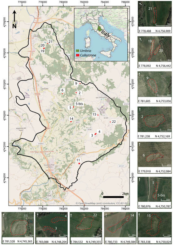
Figure 1.
The location of 14 selected shallow landslides is shown in Open Street Map. The location of Collazzone and Umbria region are shown in upper right corner of the Open Street Map. On the left side of the map and below it, the 11 images show the 14 landslides mapped (red dotted lines) on the GE image acquired on 8 April 2021, with the coordinates of the LPs center. Black and white numbers represent ID landslides and white arrows indicate north.
Climate is characterized by cold and moist winters and dry summers. Landslides are abundant and range in age, type, morphology and volume from relict—partly eroded—large and deep-seated landslides, to young, mostly shallow landslides involving the soil mantle [36]. Landslides are triggered predominantly by meteorological events, including intense and prolonged rainfall and rapid snowmelt [38]. A multi-temporal landslides inventory map [38,39] was prepared by the Geomorphology group of the CNR-IRPI research institute by photointerpretation of stereo aerial photographs taken in 1941, 1954, 1977, 1985, and 1997. From 1999 up to now, event inventories were prepared following intense and or prolonged meteorological events. The inventories were prepared using field mapping techniques or photo-interpretation of satellite images or LIDAR data [39,40,41,42]. Inspection of the inventory reveals that landslides are most abundant in the cultivated areas and are rare in the forested terrain, indicating a dependence of the landslides on agricultural practices, at least in the last 20 years. Figure 2 shows photos of three intermittent shallow landslides taken during the field surveys.
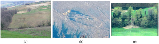
Figure 2.
Example of shallow landslides in the study area: (a) Soil slide; photo taken on 20 December 2020, by CNR-IRPI. (b) Soil slide; photo taken on 9 April 2014 by CNR-IRPI. (c) Earth flow; photo taken on 9 April 2014 by CNR-IRPI.
2.2. Methodology for Determining Occurrence of Shallow Landslides in Agricultural Environments
This paper proposed an update of the methodology, which was developed to identify buried archeological remains [26], to detect and monitor shallow landslides in agricultural environments This methodology assesses the capability of image processing products to evaluate their potential for landslide detection exploiting a parameter independent from the photo-interpreter’s skill. The methodology includes three sequential procedures (three columns in Figure 3). The schema of the updated methodology are shown in Figure 3, highlighting the data, decisions, and processes involved.
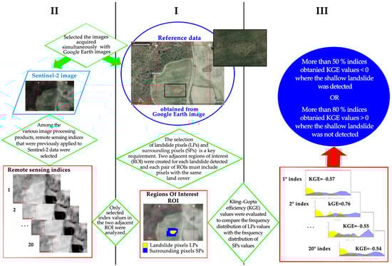
Figure 3.
The proposed methodology schema. Three sequential procedures named with Roman numerals (I–III) and divided by black lines; start datum (i.e., reference data where red circle shows the landslide) and results are in blue circles; black rectangle shows the zoom of the reference data; datum (i.e., Sentinel-2 image) is shown with a light blue trapezoid; decisions for data selection or processes are in green diamonds; the processes are shown with red rectangles. Image coordinates were expressed in decimal degrees.
2.3. First Procedure (I Panel in Figure 3)
2.3.1. Reference Data and Regions of Interest
The first procedure starts with reference data, which are essential to test and validate the entire methodology. The term validation is defined as “the process of assessing, by independent means, the quality of the data products derived from the system outputs” by the Working Group on Calibration and Validation of the Committee on Earth Observing Satellites [31]. “Reference data”, which are provided by independent means, are usually compared with processing data to assess their “degree of correctness” or accuracy [43,44]. In this work, the “means independent” of Sentinel-2 data that were employed is Google Earth (GE) images. These “independent means” allowed us to obtain the landslide inventory map (LIM) and landslide maps (LM)s, which are the reference data used in this work.
To test and validate the methodology, a LIM was prepared by the visual inspection of the very high-resolution image of the GE platform that was acquired on 8 April 2021; the inventory contains 94 shallow landslides (soil slide and earth flow). A multi-temporal analysis of GE images from both before and after the inventory map was performed and only 14 landslides were selected since their LPs and SPs were characterized by the same land cover. Table 1 summarizes the landslides that were detected using GE images.

Table 1.
Landslides detected on the five GE images. The first column shows the Landslide ID and the first row summarizes the GE acquisition date.
The multi-temporal analysis of GE images revealed 28 landslide cases (YL) and 24 no landslide cases (NL) (Table 1).
2.3.2. Regions of Interest (ROIs)
The previous paper proposing and testing the methodology to detect buried archaeological remains from remote imagery highlighted that ROI (OBARPs and SBARPs) selection is very important [26,29]. Consequently, to detect shallow landslides on the remote image, proper selection of LPs and SPs is a key requirement. The landslide pixels must accurately fit the shallow landslide shape of LIM and LMs. For this purpose, the pixels of the analyzed images were spatially resampled to 5 m. Since the primary objective of this work is to highlight the boundaries of each landslide, only the immediately surrounding pixels can identify the landslide. Moreover, to highlight only spectral differences due to landslide, LPs and SPs should only include pixels with the same land cover and land use. Therefore, LPs and SPs on Sentinel-2 images were selected by creating two adjacent ROIs according to the corresponding landslide maps and simultaneous GE images. Thanks to these images, only pixels with the same land cover and land use were selected. In Figure 3, the central green diamond underscores the requirements that guided the selection of two adjacent ROIs.
2.4. Second Procedure (II Panel in Figure 3)
2.4.1. Remote Image
The second procedure starts with the requirement for selecting Sentinel-2 images (green diamond in the upper left corner of the Figure 3) [45]: the selected images must be acquired at the same date, or nearly the same date, that the GE images were acquired (i.e., the reference data, Table 2). Only two Sentinel-2 images are acquired nearly simultaneously with the GE data (21 April 2018 and 24 March 2022).
Table 2.
GE and Sentinel-2 image acquisition dates.
Sentinel-2 is a mission developed by the European Space Agency (ESA) in the framework of the Copernicus program [46] and includes two identical satellites in the same orbit: Sentinel-2A, launched on 23 June 2015, and Sentinel-2B, launched on 7 March 2017. This mission was designed to give a high revisit frequency of 5 days at the Equator. Each satellite carries a multispectral scanner with 13 spectral bands and spatial resolutions ranging from 10 to 60 m (Table 3 [47]). Sentinel-2 images were downloaded from Copernicus Open Access Hub platform [48].
Table 3.
Main characteristics of the multispectral sensors hosted on Sentinel-2 satellites.
2.4.2. Image Processing Products Selected
The other step of the second procedure is the selection of the image processing products. The methodology for detection of the buried archeological remains was applied to many image processing products (e.g., apparent thermal inertial [26], fractional abundance images [49], principal component images [25], remote sensing indices [27,30] and rule images [28]). Since many authors detected and monitored landslides using different indices of vegetation [17,18], the proposed methodology was tested and validated by exploiting most of the remote sensing indices that were applied to Sentinel-2 data (Table 4).
Table 4.
Selected remote sensing indices.
Table 4 lists the 20 indices analyzed (i.e., 17 vegetation indices and 3 soil indices, highlighted with an asterisk in Table 4). Most of these indices were also exploited to detect the buried archeological remains [27,30]. The names and acronyms of the remote sensing indices are listed in the first and second columns, respectively; the references of the paper that proposed them and the data on which the authors tested them are listed in columns 3 and 4, respectively. Column 5 shows the equations performed on the Sentinel-2 images; the characteristics of the bands used are shown in Table 3. The works that retrieved these indices from Sentinel-2 image are shown in column 6 and most of these remote sensing indices were included in two online base dates [56,58].
The selected indices were retrieved from Sentinel-2 images using ENVI 5.6.3 © 2024 L3Harris Geospatial Solutions Inc and only selected index values include in the two adjacent ROIs were analyzed (Figure 3).
2.5. Third Procedure (III Panel in Figure 3)
Kling–Gupta Efficiency
As mentioned above, the impact of both shallow landslides and buried archeological remains on vegetation features and soil moisture distribution can be captured in images [20,23]. Therefore, within an agricultural land cover with quite homogeneous characteristics, the distinct spectral behavior of LPs and SPs enables the detection of shallow landslides images.
Therefore, by comparing the frequency distribution of LPs values with the frequency distribution of SPs values, it is possible to assess the “visibility” of a shallow landslide on the image. The Kling–Gupta efficiency (KGE) was exploited to evaluate similarity between these frequency distributions because the KGE value is used not only to calibrate and evaluate the hydrological models [72], but also to measure the similarity between spectra (e.g., [73]) and the histograms of pixel values (e.g., [44]). The KGE value is given as follows [72]:
where R is linear correlation, σ is their standard deviation, and µ represents mean values between the histograms of LPs and immediately SPs. The KGE values were classified by the literature into two classes: positive values that indicate equal, approximately similar distributions and negative values that indicate uncomparable distributions [73,74]. To compare the remote sensing indices that have different ranges of values, the values were normalized between the maximum and minimum values of overall range of values. On the other hand, to compare different shallow landslides having different sizes, the values of LPs and SPs were divided by their pixel number.
Therefore, the third procedure of the proposed methodology requires the evaluation of the KGEs for each pair of ROIs that were included in each Sentinel-2 image (Figure 4).
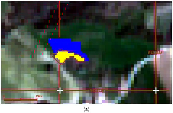
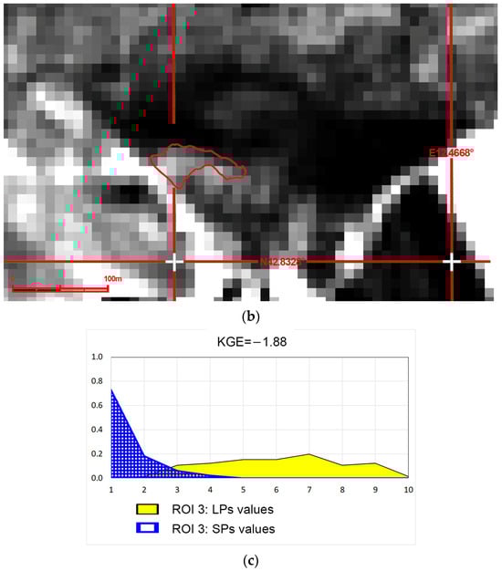
Figure 4.
The steps to calculate the values of KGE (i.e., the identification of LPs and SPs, the calculation of the remote sensing indices, and KGE evaluation). The figure shows the Landslide ID 3: (a) LPs (yellow) and SPs (blue) selected on the Sentinel-2 image acquired on 8 April 2021 and landslide track was overlaid with red circle; (b) SIPI detail on which the LM was overlaid with red circle; (c) the histograms of LP values (yellow) and SP values (blue) and their comparison yielded a KGE value of −1.88. Image coordinates were expressed in decimal degrees.
These steps were also performed in areas where landslides were not detected (NL). In these areas, we used the ROIs identified on the image acquired later or earlier, i.e., on the image where the landslide was observed.
3. Results
As above mentioned, to obtain the reference data, five GE images, which were acquired simultaneously, or nearly simultaneously, with Sentinel-2 images, were exploited and starting from the LIM of 8 April 2021, four LMs were carried out (Table 1). Since the land cover and land use of LPs and SPs must be the same, among these landslides, only 14 landslides were selected and monitored over time in the Sentinel-2 images. These 14 landslides, therefore, were monitored on 4 different days because 3 GE images covered the entire study area (25 April 2018, 8 October 2019, and 8 April 2021), whereas 2 GE images (23 March 2022, and 30 May 2023) covered only a portion of the study area (Table 2). On these days, some shallow landslides were present (YL) and some were absent (NL) (for a total of 56 study cases). However, because the LPs and SPs of four study cases revealed different land cover and land use (NMC) were not considered (Table 1). Therefore, 52 reference data were identified: 28 data include areas where landslides were detected (YL) and 24 include areas where landslides were not detected (NL, Table 1).
These reference data were used to evaluate the capability of the proposed methodology to detect shallow landslides characterized by a size comparable to or smaller than the pixel size of Sentinel-2 images. Since the Sentinel-2 sensors have three different spatial resolutions (Table 3), it is not easy to identify sizes that are comparable to spatial resolution of the sensors. Therefore, landslide sizes characterized by an LP area of 3600 m2 (i.e., the area covered by one 60 m pixel or by a 3 × 3 pixel square of 20 m) and a minimum landslide width of 20 m were defined as comparable to the spatial resolution of Sentinel-2 data. Table 5 shows the 24 selected landslides in descending order of size. The fifth column of the Table 5 indicates how we labeled the landslide size with respect to the spatial resolution of Sentinel-2 images: GT denotes a size that is larger than spatial resolution; CO denotes a size that is comparable to spatial resolution; and LT denotes a size that is smaller than spatial resolution.
Table 5.
The list in descending order of the landslide sizes detected on the GE images.
Only the Landslide ID 11 is larger than the spatial resolution of the sensors (GT), and only the Landslide ID 14 has a size that can be considered comparable (CO), whereas all the other 25 landslides have smaller sizes.
Figure 5 shows the methodology performed to detect the Landslide ID 11 (its location is shown in Figure 1). The size of this landslide is greater than the spatial resolution of the Sentinel-2 images (third column of Table 5): the minimum landslide width is 70 m; the LPs (yellow in the third row of the Figure 5) cover an area of 6250 m2 and the SPs (blue in the third row of the Figure 5) cover an area of 10,975 m2. This shallow landslide was characterized by the largest area (i.e., 6250 m2, Table 5).
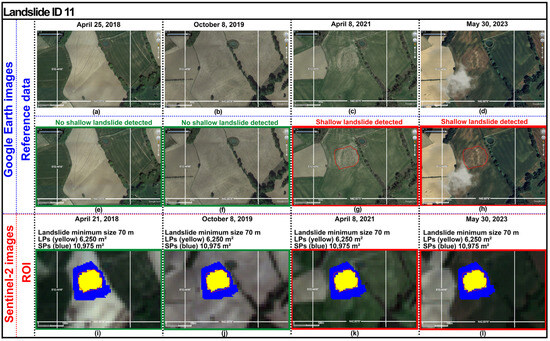
Figure 5.
Methodology for monitoring Landslide ID 11. The first row (a–d) shows the GE images. The second row (e–h) shows the reference data where red circle shows the landslide. In the third row (i–l), the yellow polygons indicate the LPs and the blue polygons indicate the SPs that were laid over Sentinel-2 images. In the second and third rows, the green frames highlight the absence of landslide evidence in the image and the red frames highlight the presence of landslide evidence in the image. Image coordinates were expressed in decimal degrees.
Figure 6 shows the methodology performed to detect the Landslide ID 14 (the location is shown in Figure 1). The size of this landslide can be considered comparable to the spatial resolution of the Sentinel-2 images (third column of Table 5): the minimum landslide width is 25 m; the LPs (yellow polygons in the third row of Figure 6) cover an area of 2250 m2 and the SPs (blue polygons in the third row of Figure 6) cover an area of 6150 m2.
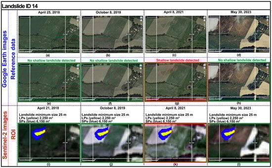
Figure 6.
Methodology for monitoring Landslide ID 14. The first row (a–d) shows the GE images. The second row (e–h) shows the reference data where red circle shows the landslide. In the third row (i–l), the yellow polygons indicate the LPs and the blue polygons indicate the SPs that were laid over Sentinel-2 images. In the second and third rows, the green frames highlight the absence of landslide evidence in the image and the red frames highlight the presence of landslide evidence in the image. Image coordinates were expressed in decimal degrees.
In Figure 5 and Figure 6, the results in the columns are sorted based on image acquisition dates, and the results in the rows obtained are sorted with respect to the steps of the first procedure. According to image acquisition dates, the first, and second rows show GE images and LMs superimposed on GE images, and the third row shows ROIs superimposed on the Sentinel-2 images. In other words, in the same column, GE images and LMs derived from these were compared with Sentinel-2 images acquired immediately or nearly simultaneously with the first ones. The details of the GE images associated with the landslide are shown in the first rows of Figure 5 and Figure 6. The second rows of Figure 5 and Figure 6 display the details of LMs. The third rows of Figure 5 and Figure 6 show LPs and SPs, which were marked out on the Sentinel-2 images, and display information about their size. In the second and third rows, red frames show the areas where the landslides were detected (YL in the Table 1), whereas green frames highlight the areas where the landslides were not detected (NL in the Table 1). As mentioned above, in the Sentinel-2 images where no landslides were detected, we utilized the ROIs that were identified in the next or previous image where a landslide was detected. For instance, as regarding the Landslide ID 11, ROIs identified on the Sentinel-2 image acquired on 8 April 2021 were used to analyze Sentinel-2 images acquired on 21 April 2018 and 8 October 2019 (Figure 5).
After the first procedure was completed, selected remote sensing indices were retrieved from Sentinel-2 images, and then, KGE values were calculated for each ROI and each image. Figure 7a,b show 160 values of KGE obtained to detect Landslide IDs 11 and 14, respectively. Different colored columns show the twenty KGE values obtained from the four images: the red, green, yellow, and blue bars show the KGE values obtained from Sentinel-2 images acquired on 30 May 2023, 8 April 2021, 8 October 2019, and 21 April 2018.
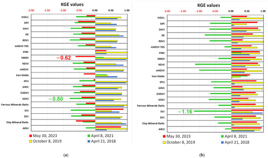
Figure 7.
KGE values, shown on the x-axis, calculated from remote sensing indices obtained from Sentinel-2 images, which were highlighted on the y-axis: (a) KGE values calculated from the indices to monitor the Landslide ID 11. The minor values of KGE were highlighted; (b) KGE values calculated from the indices to monitor the Landslide ID 14. The minor value of KGE was highlighted.
These KGE values quantified the ability of each remote sensing indices to detect these two landslides: one with the sizes greater than the spatial resolution of Sentinel-2 images (Landside ID 11) and the other with the sizes comparable to the spatial resolution of images (Landside ID 14). GDVI and NMDI are two indices that most emphasized Landslide ID 11 on the Sentinel-2 images acquired on 8 April 2021 and 30 May 2023, respectively. The KGE values are equal to −0.80 and −0.62, respectively (Figure 7a). EVI is the index that most emphasized Landslide ID 14 on the Sentinel-2 images acquired on 8 April 2021. The KGE value is equal to −1.16 (Figure 7b).
Figure 8 and Figure 9 compared three different index zooms portraying the Landslides IDs 11 and 14, respectively: one index obtained the minimum value (Figure 8c–f and Figure 9c–f), one obtained a value close to zero (Figure 8b–e and Figure 9b–e), and one index obtained a value greater than zero (Figure 8a–d and Figure 9a–d). The purpose of these figures is to identify KGE values that detect shallow landslides (i.e., KGE ≤ 0) and KGE values that do not detect landslides (i.e., KGE > 0).
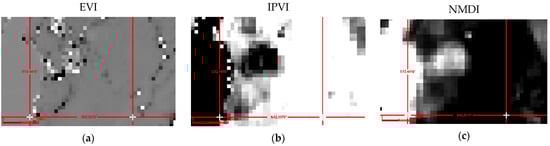
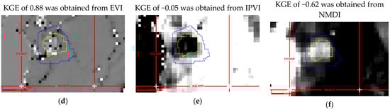
Figure 8.
KGE values obtained from indices that were retrieved from Sentinel-2 image of 30 May 2023 for Landslide ID 11: (a) EVI; (b) IPVI; (c) NMDI; (d) the edges of LPs (yellow) SPs (blue) superimposed on EVI; (e) the edges superimposed on IPVI; (f) the edges superimposed on NMDI. Image coordinates were expressed in decimal degrees.
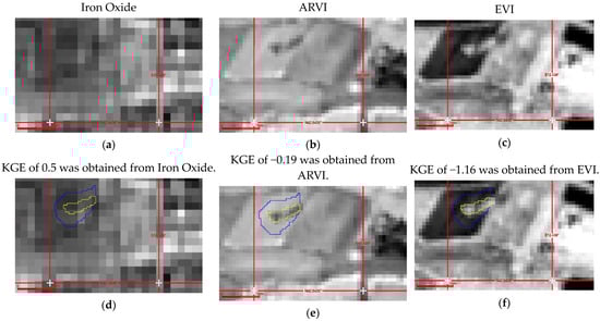
Figure 9.
KGE values obtained from indices that were retrieved from Sentinel-2 image of 8 April 2021 for Landslide ID 14 in Figure 1: (a) Iron Oxide; (b) ARVI; (c) EVI; (d) the edges of LPs (yellow) SPs (blue) superimposed on Iron Oxide; (e) the edges superimposed on ARVI; (f) the edges superimposed on EVI. Image coordinates were expressed in decimal degrees.
Regarding the Landslide ID 11, Figure 8 show three indices that were obtained from the images acquired on 30 May 2023: EVI with KGE value of 0.88, IPVI with KGE value of −0.05, and NMDI with KGE value of −0.62. Regarding the Landslide ID 14, Figure 9 shows three indices that were obtained from the images acquired on 8 April 2021: Iron Oxide with KGE value of 0.5, ARVI with KGE value of −0.19, and EVI with KGE value of −1.16.
The comparison of the indices confirms that where KGE values are greater than zero, the landslide is undetectable (Figure 8a,d and Figure 9a,d), whereas where KGE values are less than zero landslide is detectable (Figure 8b,c,e,f and Figure 9b,c,e,f). It is important to highlight that Figure 8b,e and Figure 9b,e show that the landslide is detectable not only where KGE values are less than zero, but also where KGE values are close to zero. In addition, a decrease in KGE value allows the landslide to be more detectable.
We considered “true positive” the landslide case in which the index confirms the presence of the landslide (YL) and “true negative” the case in which the index confirms the absence of the landslide (NL). On the other hand, we considered “false negative” the case in which the index does not confirm the presence of the landslide and “false positive” the case in which the index does not confirm the absence of the landslide.
Regarding the Landslide ID 11, seventeen values of KGE less than zero were obtained from the images acquired on 8 April 2021 and 30 May 2023 (17 true positive of 20). Regarding the image acquired on 8 April 2021, Iron Oxide, NMDI, and PSRI are the indices that obtained the “false negative” with respect to reference maps where landslides were detected (i.e., 0.4, 0.3, and 0.0, respectively, Figure 7a). Regarding the image acquired on 30 May 2023, ARVI, EVI, and PSRI are the indices that obtained the “false negative” (i.e., 0.8, 0.9, and 0.3, respectively). Regarding the Landslide ID 14, eighteen values of KGE less than zero were obtained from the image acquired on 8 April 2021 (18 true positive of 20). Iron Oxide, and PSRI are the indices that obtained the “false negative” (i.e., 0.5, and 0.3, respectively, Figure 7b). On the other hand, each KGE value in images where landslides were not detected is greater than zero (20 true negative of 20). No landslide was detected from the indices obtained from images corresponding to reference maps where no landslide was detected.
Figure 10 shows the methodology performed and the results obtained to monitor the Landslide ID 4. The size of the Landslide ID 4, which was detected on the image acquired on 25 April 2018, was the smallest of those analyzed (Table 5).
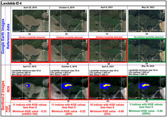
Figure 10.
Methodology for monitoring Landslide ID 4. The first row (a–d) shows the GE images. The second row (e–h) shows the reference data where red circle shows the landslide. In the third row (i–l), the yellow polygons indicate the LPs and the blue polygons indicate the SPs that were laid over Sentinel-2 images. In the second and third rows, the green frames highlight the absence of landslide evidence in the image and the red frames highlight the presence of landslide evidence in the image The last row summarizes the KGE values obtained for each image. Image coordinates were expressed in decimal degrees.
Also in Figure 10, the horizontal rows subdivide the results obtained with respect to the steps of the first procedure, whereas the columns sort the results obtained with respect to the sensor acquisition dates. The first row shows the details of GE images related to the landslide; the second row displays the details of LMs overlaid on GE images. The third row shows LPs and SPs, which were marked out on the Sentinel-2 images, and display information about their size. In the second and third rows, red frames highlight the areas where the landslides were detected, whereas green frames highlight the areas where the landslides were not detected. The fourth row summarizes the results obtained from the four Sentinel-2 images showing negative value of KGEs. These results also highlighted that most of the KGE values are negative in images corresponding to reference maps where the landslides were detected (YL). Sixteen negative values of KGE (16 true negative) were obtained from the Sentinel-2 images acquired on 8 April 2021, and four false negatives were obtained (see Figure A14 in Appendix B). Eleven values of KGE minor than zero (11 true negative) were obtained from the images acquired on 21 April 2018, and 8 October 2019, and nine false negatives were obtained (see Figure A14 in Appendix B).
On the other hand, most of KGE values are greater than zero from images corresponding to reference maps where no landslides were detected (NL). Three false positives were obtained from the images acquired on 30 May 2023 (Figure A14 in Appendix B). Figure 11 summarizes the numbers of true positive and true negative that were obtained for each landslide.
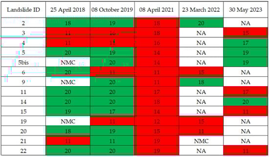
Figure 11.
Green cell means NL and the figures are the number of indices that confirmed no landslide presence (i.e., true negative). Red cell means YL and the figures are the number of indices that confirmed landslide presence (i.e., true positive). NA: image not available. NMC: LPs and SPs characterized by the different land cover in that image.
In conclusion, most indices yield true positives (70%) and true negatives (94%).
In Appendix A, the Figure A1, Figure A2, Figure A3, Figure A4, Figure A5, Figure A6, Figure A7, Figure A8, Figure A9, Figure A10 and Figure A11 show the methodology performed to monitor the other landslides and, in Appendix B, Figure A12, Figure A13, Figure A14, Figure A15, Figure A16, Figure A17, Figure A18, Figure A19, Figure A20, Figure A21, Figure A22 and Figure A23 show the KGE values obtained.
The overall accuracy of each index, calculated to distinguish areas where shallow landslides are present from those where they are absent, was given as follows [75]:
where TP is equal to true positive, FP is equal to false positive, FN is equal to false negative, and FP is equal to false positive. Moreover, to validate the performance of the indices, the precision was calculated using Sørensen–Dice index (SDI) according to [76,77]:
Table 6 lists the indices according to their values of overall accuracy and precision that are shown in the second and third columns, respectively.
Table 6.
The overall accuracy and precision values of selected indices.
The first column of Table 6 shows the acronym of the index and the eighth column shows the spatial resolution of the bands used to calculate it. The fourth column shows the number of the true positive. The seventh column shows the number of the true negative. The fifth and sixth columns show the average value and the minimum value of the KGE obtained.
The overall accuracy and precision analysis highlighted that only SAVI, and RDVI obtained a value equal to 1, followed by GRVI and NDVI which obtained values equal to 0.98, whereas ARVI obtained an accuracy equal to 0.56 and SDI value equal to 0.38.
Regarding the number of the true positive (i.e., the ability to detect the landslides), the third column of Table 6 shows that SAVI, RDVI, and SIPI detected 100% of the landslides followed by GRDVI and NDVI which detected 96% of the shallow landslides, whereas ARVI detected 24% of the shallow landslides. Analyzing these values also shows that every index detected an average of 69% of landslides (i.e., about 19 landslides out of 28).
Regarding the mean values of KGE, the fourth column displays that the lowest mean value (i.e., −0.57) was retrieved from mNDVI index, following by the mean values obtained from DVI, EVI and NDVI (about −0.50); the highest mean value (i.e., −0.22) was retrieved from PSRI and the ferrous minerals ratio. Concerning the minimum values of KGE, the fifth column shows that the lowest minimum values were retrieved from SIPI and NDVI (i.e., −1.88 and −1.68, respectively), followed by the minimum values obtained from mMDVI, and clay mineral ratio (i.e., −1,44); the highest minimum value was retrieved from PSRI index (i.e., −0.57). Regarding true negatives (i.e., the ability to monitor the landslides), all indices do not identify landslides where they are not present, resulting in 94% true negatives.
4. Discussion and Conclusions
To detect shallow landslides in agricultural environments in the remote images, this research exploited some characteristics that the shallow landslides shared with buried archaeological remains. Both landslides and buried structures alter the flow of surface water, creating anomalies in soil moisture content [20,21,23]. In remote images, this results in a difference in the spectral features of landslide pixels (LPs) or OBARPs (in the case of buried structures) and non-landslide pixels (SPs) or SBARPs (in the case of buried structures). However, the sizes of the shallow landslides are often comparable to or smaller than the spatial resolution of remote images, whereas the sizes of buried archaeological remains are often comparable to or greater than the spatial resolution of remote images. Additionally, landslides change over time due to factors such as rainfall and human activity, which alter their presence, shape, and size. Therefore, to enhance the detection and monitoring of shallow landslides, this research proposes an update of the methodology that was previously tested and validated for detecting numerous buried archaeological remains [26,30]. Remote sensing is widely used to monitor most environmental parameters and phenomena (e.g., [78,79]). Identifying shallow landslides is crucial in rural areas, where records of such events are sparse. Small-scale events are most often restored and cleared by farmers to make the land usable again. It is noteworthy that not only the scientific community, but also the policy-making community, recognize the importance of monitoring phenomena and processes [80]. Additionally, many papers monitoring environmental phenomena and parameters have utilized the Sentinel-2 sensors [78,79,80].
To detect known shallow landslides over time, this paper introduces an updated methodology that assesses not only areas where shallow landslides are present, but also areas where shallow landslides are not present. The large percentages of true positives (70%) and true negatives (94%) highlight the robustness of the methodology in monitoring landslides over time.
In previous studies on shallow landslides, authors detected them using photo-interpretation of images and/or NDVI [2,3] and developed semi-automatic methods based on change detection approaches in events where landslides with long-runout completely modified land cover (e.g., from vegetation to bare ground) [2,4,17].
The shallow landslides in agricultural environments analyzed are characterized by short-runout and low mobilization rate [20]. Therefore, the spectral characteristics of the LPs are comparable to those of SPs. This work does not rely on change detection, which takes advantage of the difference in pixel values in the images pre and post landslide, but it compares pixel values inside and outside the landslide boundary in the same image.
The results show that the proposed methodology successfully allows for monitoring of known shallow landslides, which have dimensions comparable to or smaller than the pixel size of Sentinel-2 images (Table 5). The percentages of true positives and true negatives that were obtained for landslides characterized by sizes smaller than the spatial resolution of Sentinel-2 images are equal to 68% and 93%, respectively.
The methodology was validated using 52 reference data related to 14 shallow landslides monitored over time for a total of 28 landslide cases (YL) and 24 no landslide cases (NL, Table 1). In accordance with the validation requirements, the reference data were obtained from the GE images that have a higher spatial resolution than Sentinel-2 images and GE images were acquired simultaneously or nearly simultaneously with the Sentinel-2 images [43,44]. Moreover, photo-interpretation of the GE images was carried out by experienced photo-interpreters.
To test the methodology, 20 remote sensing indices were selected (Table 6). To rank the detection capability of the indices, the methodology calculated the parameter (i.e., the KGE value) independent of the photo-interpreter’s skill. The KGE values revealed that landslides are visible when the KGE value is equal to or less than zero, confirming previous literature findings [73,74,81]. In evaluating the capability of each index, overall accuracy and precision [75,76,77] were assessed. The analysis of overall accuracy values shows that two indices reveal an accuracy equal to 1 (i.e., SAVI and RDVI) and six obtained the values greater than 0.90 (i.e., GRVI, NDVI, SIPI, GNDVI, DVI, and SR), whereas ARVI reveals the accuracy value equal to 0.56.
The analysis of precision values shows that two indices reveal a precision equal to 1 (i.e., SAVI and RDVI) and six obtained values greater than 0.90 (i.e., GRVI, NDVI, SIPI, GNDVI, DVI, and SR), whereas PSRI and ARVI reveal values less than 0.5. These values highlight that not only the NDVI, but also other indices, are able to detect shallow landslides and that all contribute to monitoring them over time.
The studies conducted on the detection of buried archeological remains highlighted that not all image processing products can be successfully applied to all case studies, since the capability to detect them on image depends on many factors [26,30]. Therefore, the likelihood of detecting buried archaeological remains increases with the number of image processing products evaluated. These studies confirm the findings that emerged from the detection of shallow landslides and emphasizes the importance of analyzing many image processing products for successful detection and monitoring of shallow landslides.
Among the indices selected and used, seventeen are vegetation indices and three are soil indices. Vegetation indices were more able to distinguish landslide areas from non-landslide areas (mean overall accuracy is equal to 0.85 and mean precision is equal to 0.82) than soil indices (mean overall accuracy is equal to 0.70 and mean precision is equal to 0.63). In this study, the overall accuracy and the precision are also influenced by the resolution of the bands used. Specifically, soil indices use bands with resolutions of 20–60 m, whereas vegetation indices mainly use bands with resolutions of 10–20 m. Notably, the soil indices can detect landslides larger than 60 m resolution (Landslide ID 11) but they failed for landslides smaller than 3600 m2.
This methodology can work on other environments, as long as each LP and SP pair is characterized by the same land cover and land use.
The following strengths were identified using the suggested methodology: (i) the use of free satellite images, such as Sentinel-2 images that are available under credentials at the platform https://www.sentinel-hub.com/ (accessed on 19 April 2022), a resource for monitoring events over time; (ii) using reference data as a starting point; (iii) the calculation of many indices allowing for the identification of shallow landslides whose dimensions are smaller than the spatial resolution of the images; (iv) the calculation of many indices allowing for the identification of landslides that did not produce changes in land cover; (v) the use of the KGE parameter allowing for the ranking of index ability on landslide detection. However, additional research is needed to develop an automated procedure to improve the continuous monitoring of known landslides after triggering events.
The quantitative results of the presented work show the proposed methodology’s success in its intended objective. It also revealed the capability of many indices to identify small and shallow landslides in agricultural environments where their detection is difficult due to intermittent landslides caused by ploughing activity. In this way, the results extend the use of remote sensing indices not only where the signal caused by a landslide is evident and results in a change in land cover, but also when the marks are very subtle or almost absent.
These findings support ongoing research, with the intention to assess the methodology in different study areas and with different image processing products. Efforts are underway to develop a semi-automated approach integrating the time-consuming tasks of image acquisition, processing, index computation, and KGE analysis.
Author Contributions
Conceptualization, R.M.C.; methodology, R.M.C.; image processing R.M.C., and F.A.; data analysis, R.M.C. and L.P.; validation, R.M.C., F.F. and F.A.; writing—original draft preparation, R.M.C. and F.A.; writing—review and editing, R.M.C., L.P., F.F. and F.A. All authors have read and agreed to the published version of the manuscript.
Funding
This research received no external funding.
Data Availability Statement
Data are contained within the article.
Acknowledgments
The authors thank two anonymous reviewers for improving the quality of the manuscript with their comments and suggestions.
Conflicts of Interest
The authors declare no conflicts of interest.
Appendix A
The Figure A1, Figure A2, Figure A3, Figure A4, Figure A5, Figure A6, Figure A7, Figure A8, Figure A9, Figure A10 and Figure A11 show the methodology performed and results obtained to detect the landslides that were marked with the numbers 2, 3, 5, 5bis, 6, 9, 15, 19, 20, 21, and 22 in Figure 1, except for Landslides ID 4, 11, and 14, which are shown in Figure 5, Figure 6 and Figure 10.

Figure A1.
Methodology for monitoring Landslide ID 2. The first row (a–d) shows the GE images. The second row (e–h) shows the reference data where red circle shows the landslide. In the third row (i–l), the yellow polygons indicate the LPs and the blue polygons indicate the SPs that were laid over Sentinel-2 images. In the second and third rows, the green frames highlight the absence of landslide evidence in the image and the red frames highlight the presence of landslide evidence in the image. The last row summarizes the KGE values obtained for each image. Image coordinates were expressed in decimal degrees.


Figure A2.
Methodology for monitoring Landslide ID 3. The first row (a–d) shows the GE images. The second row (e–h) shows the reference data where red circle shows the landslide. In the third row (i–l), the yellow polygons indicate the LPs and the blue polygons indicate the SPs that were laid over Sentinel-2 images. In the second and third rows, the green frames highlight the absence of landslide evidence in the image and the red frames highlight the presence of landslide evidence in the image.. The last row summarizes the KGE values obtained for each image. Image coordinates were expressed in decimal degrees.


Figure A3.
Methodology for monitoring Landslide ID 5. The first row (a–d) shows the GE images. The second row (e–h) shows the reference data where red circle shows the landslide. In the third row (i–l), the yellow polygons indicate the LPs and the blue polygons indicate the SPs that were laid over Sentinel-2 images. In the second and third rows, the green frames highlight the absence of landslide evidence in the image and the red frames highlight the presence of landslide evidence in the image. The last row summarizes the KGE values obtained for each image. Image coordinates were expressed in decimal degrees.


Figure A4.
Methodology for monitoring Landslide ID 5 bis. The first row (a–c) shows the GE images. The second row (d–f) shows the reference data where red circle shows the landslide. In the third row (g–i), the yellow polygons indicate the LPs and the blue polygons indicate the SPs that were laid over Sentinel-2 images. In the second and third rows, the green frames highlight the absence of landslide evidence in the image and the red frames highlight the presence of landslide evidence in the image. Green frames highlight the absence of landslide evidence and the red frames highlight the presence of landslide evidence in the image. The last row summarizes the KGE values obtained for each image. Image coordinates were expressed in decimal degrees.


Figure A5.
Methodology for monitoring Landslide ID 6. The first row (a–d) shows the GE images. The second row (e–h) shows the reference data where red circle shows the landslide. In the third row (i–l), the yellow polygons indicate the LPs and the blue polygons indicate the SPs that were laid over Sentinel-2 images. In the second and third rows, the green frames highlight the absence of landslide evidence in the image and the red frames highlight the presence of landslide evidence in the image. The last row summarizes the KGE values obtained for each image. Image coordinates were expressed in decimal degrees.


Figure A6.
Methodology for monitoring Landslide ID 9. The first row (a–c) shows the GE images. The second row (d–f) shows the reference data where red circle shows the landslide. In the third row (g–i), the yellow polygons indicate the LPs and the blue polygons indicate the SPs that were laid over Sentinel-2 images. In the second and third rows, the green frames highlight the absence of landslide evidence in the image and the red frames highlight the presence of landslide evidence in the image The last row summarizes the KGE values obtained for each image. Image coordinates were expressed in decimal degrees.


Figure A7.
Methodology for monitoring Landslide ID 15. The first row (a–d) shows the GE images. The second row (e–h) shows the reference data where red circle shows the landslide. In the third row (i–l), the yellow polygons indicate the LPs and the blue polygons indicate the SPs that were laid over Sentinel-2 images. In the second and third rows, the green frames highlight the absence of landslide evidence in the image and the red frames highlight the presence of landslide evidence in the image. The last row summarizes the KGE values obtained for each image. Image coordinates were expressed in decimal degrees.


Figure A8.
Methodology for monitoring Landslide ID 19. The first row (a–c) shows the GE images. The second row (d–f) shows the reference data where red circle shows the landslide. In the third row (g–i), the yellow polygons indicate the LPs and the blue polygons indicate the SPs that were laid over Sentinel-2 images. In the second and third rows, the green frames highlight the absence of landslide evidence in the image and the red frames highlight the presence of landslide evidence in the image. The last row summarizes the KGE values obtained for each image. Image coordinates were expressed in decimal degrees.


Figure A9.
Methodology for monitoring Landslide ID 20. The first row (a–d) shows the GE images. The second row (e–h) shows the reference data where red circle shows the landslide. In the third row (i–l), the yellow polygons indicate the LPs and the blue polygons indicate the SPs that were laid over Sentinel-2 images. In the second and third rows, the green frames highlight the absence of landslide evidence in the image and the red frames highlight the presence of landslide evidence in the image. The last row summarizes the KGE values obtained for each image. Image coordinates were expressed in decimal degrees.


Figure A10.
Methodology for monitoring Landslide ID 21. The first row (a–c) shows the GE images. The second row (d–f) shows the reference data where red circle shows the landslide. In the third row (g–i), the yellow polygons indicate the LPs and the blue polygons indicate the SPs that were laid over Sentinel-2 images. In the second and third rows, the green frames highlight the absence of landslide evidence in the image and the red frames highlight the presence of landslide evidence in the image. The last row summarizes the KGE values obtained for each image. Image coordinates were expressed in decimal degrees.


Figure A11.
Methodology for monitoring Landslide ID 22. The first row (a–d) shows the GE images. The second row (e–h) shows the reference data where red circle shows the landslide. In the third row (i–l), the yellow polygons indicate the LPs and the blue polygons indicate the SPs that were laid over Sentinel-2 images. In the second and third rows, the green frames highlight the absence of landslide evidence in the image and the red frames highlight the presence of landslide evidence in the image. The last row summarizes the KGE values obtained for each image. Image coordinates were expressed in decimal degrees.

Appendix B
The KGE values obtained to detect and monitor the landslides that were marked with the 2, 3, 4, 5, 5bis, 6, 9, 15, 19, 20, 21, and 22 numbers in Figure 1, except for the Landslides ID 11 and 14 that are shown in Figure 7a,b.

Figure A12.
KGE values calculated from the indices to monitor the Landslide ID 2. Values of KGE, shown on the x-axis, calculated from remote sensing indices obtained from Sentinel-2 images, which were highlighted on the y-axis. The lowest value of KGE was highlighted.
Figure A12.
KGE values calculated from the indices to monitor the Landslide ID 2. Values of KGE, shown on the x-axis, calculated from remote sensing indices obtained from Sentinel-2 images, which were highlighted on the y-axis. The lowest value of KGE was highlighted.


Figure A13.
KGE values calculated from the indices to monitor the Landslide ID 3. Values of KGE, shown on the x-axis, calculated from remote sensing indices obtained from Sentinel-2 images, which were highlighted on the y-axis. The lowest values of KGE were highlighted.
Figure A13.
KGE values calculated from the indices to monitor the Landslide ID 3. Values of KGE, shown on the x-axis, calculated from remote sensing indices obtained from Sentinel-2 images, which were highlighted on the y-axis. The lowest values of KGE were highlighted.


Figure A14.
KGE values calculated from the indices to monitor the Landslide ID 4. Values of KGE, shown on the x-axis, calculated from remote sensing indices obtained from Sentinel-2 images, which were highlighted on the y-axis. The lowest values of KGE were highlighted.
Figure A14.
KGE values calculated from the indices to monitor the Landslide ID 4. Values of KGE, shown on the x-axis, calculated from remote sensing indices obtained from Sentinel-2 images, which were highlighted on the y-axis. The lowest values of KGE were highlighted.


Figure A15.
KGE values calculated from the indices to monitor the Landslide ID 5. Values of KGE, shown on the x-axis, calculated from remote sensing indices obtained from Sentinel-2 images, which were highlighted on the y-axis. The lowest value of KGE was highlighted.
Figure A15.
KGE values calculated from the indices to monitor the Landslide ID 5. Values of KGE, shown on the x-axis, calculated from remote sensing indices obtained from Sentinel-2 images, which were highlighted on the y-axis. The lowest value of KGE was highlighted.


Figure A16.
KGE values calculated from the indices to monitor the Landslide ID 5bis. Values of KGE, shown on the x-axis, calculated from remote sensing indices obtained from Sentinel-2 images, which were highlighted on the y-axis. The lowest values of KGE were highlighted.
Figure A16.
KGE values calculated from the indices to monitor the Landslide ID 5bis. Values of KGE, shown on the x-axis, calculated from remote sensing indices obtained from Sentinel-2 images, which were highlighted on the y-axis. The lowest values of KGE were highlighted.


Figure A17.
KGE values calculated from the indices to monitor the Landslide ID 6. Values of KGE, shown on the x-axis, calculated from remote sensing indices obtained from Sentinel-2 images, which were highlighted on the y-axis. The lowest values of KGE were highlighted.
Figure A17.
KGE values calculated from the indices to monitor the Landslide ID 6. Values of KGE, shown on the x-axis, calculated from remote sensing indices obtained from Sentinel-2 images, which were highlighted on the y-axis. The lowest values of KGE were highlighted.


Figure A18.
KGE values calculated from the indices to monitor the Landslide ID 9. Values of KGE, shown on the x-axis, calculated from remote sensing indices obtained from Sentinel-2 images, which were highlighted on the y-axis. The lowest value of KGE was highlighted.
Figure A18.
KGE values calculated from the indices to monitor the Landslide ID 9. Values of KGE, shown on the x-axis, calculated from remote sensing indices obtained from Sentinel-2 images, which were highlighted on the y-axis. The lowest value of KGE was highlighted.


Figure A19.
KGE values calculated from the indices to monitor the Landslide ID 15. Values of KGE, shown on the x-axis, calculated from remote sensing indices obtained from Sentinel-2 images, which were highlighted on the y-axis. The lowest values of KGE were highlighted.
Figure A19.
KGE values calculated from the indices to monitor the Landslide ID 15. Values of KGE, shown on the x-axis, calculated from remote sensing indices obtained from Sentinel-2 images, which were highlighted on the y-axis. The lowest values of KGE were highlighted.


Figure A20.
KGE values calculated from the indices to monitor the Landslide ID 19. Values of KGE, shown on the x-axis, calculated from remote sensing indices obtained from Sentinel-2 images, which were highlighted on the y-axis. The lowest values of KGE were highlighted.
Figure A20.
KGE values calculated from the indices to monitor the Landslide ID 19. Values of KGE, shown on the x-axis, calculated from remote sensing indices obtained from Sentinel-2 images, which were highlighted on the y-axis. The lowest values of KGE were highlighted.


Figure A21.
KGE values calculated from the indices to monitor the Landslide ID 20. Values of KGE, shown on the x-axis, calculated from remote sensing indices obtained from Sentinel-2 images, which were highlighted on the y-axis. The lowest values of KGE were highlighted.
Figure A21.
KGE values calculated from the indices to monitor the Landslide ID 20. Values of KGE, shown on the x-axis, calculated from remote sensing indices obtained from Sentinel-2 images, which were highlighted on the y-axis. The lowest values of KGE were highlighted.


Figure A22.
KGE values calculated from the indices to monitor the Landslide ID 21. Values of KGE, shown on the x-axis, calculated from remote sensing indices obtained from Sentinel-2 images, which were highlighted on the y-axis. The lowest values of KGE were highlighted.
Figure A22.
KGE values calculated from the indices to monitor the Landslide ID 21. Values of KGE, shown on the x-axis, calculated from remote sensing indices obtained from Sentinel-2 images, which were highlighted on the y-axis. The lowest values of KGE were highlighted.


Figure A23.
KGE values calculated from the indices to monitor the Landslide ID 22. Values of KGE, shown on the x-axis, calculated from remote sensing indices obtained from Sentinel-2 images, which were highlighted on the y-axis. The lowest values of KGE were highlighted.
Figure A23.
KGE values calculated from the indices to monitor the Landslide ID 22. Values of KGE, shown on the x-axis, calculated from remote sensing indices obtained from Sentinel-2 images, which were highlighted on the y-axis. The lowest values of KGE were highlighted.

References
- Cardinali, M.; Galli, M.; Guzzetti, F.; Ardizzone, F.; Reichenbach, P.; Bartoccini, P. Rainfall Induced Landslides in December 2004 in South-Western Umbria, Central Italy: Types, Extent, Damage and Risk Assessment. Nat. Hazards Earth Syst. Sci. 2006, 6, 237–260. [Google Scholar] [CrossRef]
- Mondini, A.C.; Viero, A.; Cavalli, M.; Marchi, L.; Herrera, G.; Guzzetti, F. Comparison of Event Landslide Inventories: The Pogliaschina Catchment Test Case, Italy. Nat. Hazards Earth Syst. Sci. 2014, 14, 1749–1759. [Google Scholar] [CrossRef]
- Fiorucci, F.; Ardizzone, F.; Mondini, A.C.; Viero, A.; Guzzetti, F. Visual Interpretation of Stereoscopic NDVI Satellite Images to Map Rainfall-Induced Landslides. Landslides 2019, 16, 165–174. [Google Scholar] [CrossRef]
- Notti, D.; Cignetti, M.; Godone, D.; Giordan, D. Semi-Automatic Mapping of Shallow Landslides Using Free Sentinel-2 and Google Earth Engine. Nat. Hazards Earth Syst. Sci. Discuss. 2022, 23, 2625–2648. [Google Scholar] [CrossRef]
- Prakash, N.; Manconi, A.; Loew, S. A New Strategy to Map Landslides with a Generalized Convolutional Neural Network. Sci. Rep. 2021, 11, 9722. [Google Scholar] [CrossRef] [PubMed]
- Ghorbanzadeh, O.; Gholamnia, K.; Ghamisi, P. The Application of ResU-Net and OBIA for Landslide Detection from Multi-Temporal Sentinel-2 Images. Big Earth Data 2022, 7, 961–985. [Google Scholar] [CrossRef]
- Nava, L.; Bhuyan, K.; Meena, S.R.; Monserrat, O.; Catani, F. Rapid Mapping of Landslides on SAR Data by Attention U-Net. Remote Sens. 2022, 14, 1449. [Google Scholar] [CrossRef]
- Handwerger, A.L.; Jones, S.Y.; Amatya, P.; Kerner, H.R.; Kirschbaum, D.B.; Huang, M.-H. Strategies for Landslide Detection Using Open-Access Synthetic Aperture Radar Backscatter Change in Google Earth Engine. Nat. Hazards Earth Syst. Sci. Discuss. 2021, 22, 753–773. [Google Scholar] [CrossRef]
- Mondini, A.C.; Guzzetti, F.; Chang, K.-T.; Monserrat, O.; Martha, T.R.; Manconi, A. Landslide Failures Detection and Mapping Using Synthetic Aperture Radar: Past, Present and Future. Earth-Sci. Rev. 2021, 216, 103574. [Google Scholar] [CrossRef]
- Juhadi, J.; Banowati, E.; Sanjoto, T.B.; Nugraha, S.B. Rapid Appraisal for Agricultural Land Utilization in the Erosion and Landslide Vulnerable Mountainous Areas of Kulonprogo Regency, Indonesia. Manag. Environ. Qual. Int. J. 2020, 31, 1–17. [Google Scholar] [CrossRef]
- Mauri, L.; Straffelini, E.; Cucchiaro, S.; Tarolli, P. UAV-SfM 4D Mapping of Landslides Activated in a Steep Terraced Agricultural Area. J. Agric. Eng. 2021, 52, 11–30. [Google Scholar] [CrossRef]
- Pijl, A.; Quarella, E.; Vogel, T.A.; D’Agostino, V.; Tarolli, P. Remote Sensing vs. Field-Based Monitoring of Agricultural Terrace Degradation. Int. Soil. Water Conserv. Res. 2021, 9, 1–10. [Google Scholar] [CrossRef]
- Fiorucci, F.; Giordan, D.; Santangelo, M.; Dutto, F.; Rossi, M.; Guzzetti, F. Criteria for the Optimal Selection of Remote Sensing Optical Images to Map Event Landslides. Nat. Hazards Earth Syst. Sci. 2018, 18, 405–417. [Google Scholar] [CrossRef]
- Mohd Salleh, M.R.; Ishak, N.I.; Razak, K.A.; Abd Rahman, M.Z.; Asmadi, M.A.; Ismail, Z.; Abdul Khanan, M.F. Geospatial approach for landslide activity assessment and mapping based on vegetation anomalies. Int. Arch. Photogramm. Remote Sens. Spat. Inf. Sci. 2018, 42, 201–215. [Google Scholar] [CrossRef]
- Miller, A.J. Remote Sensing Proxies for Deforestation and Soil Degradation in Landslide Mapping: A Review: Remote Sensing Proxies. Geogr. Compass 2013, 7, 489–503. [Google Scholar] [CrossRef]
- Guo, X.; Guo, Q.; Feng, Z. Detecting the Vegetation Change Related to the Creep of 2018 Baige Landslide in Jinsha River, SE Tibet Using SPOT Data. Front. Earth Sci. 2021, 9, 706998. [Google Scholar] [CrossRef]
- Mondini, A.C.; Guzzetti, F.; Reichenbach, P.; Rossi, M.; Cardinali, M.; Ardizzone, F. Semi-Automatic Recognition and Mapping of Rainfall Induced Shallow Landslides Using Optical Satellite Images. Remote Sens. Environ. 2011, 115, 1743–1757. [Google Scholar] [CrossRef]
- Mwaniki, M.W.; Kuria, D.N.; Boitt, M.K.; Ngigi, T.G. Image Enhancements of Landsat 8 (OLI) and SAR Data for Preliminary Landslide Identification and Mapping Applied to the Central Region of Kenya. Geomorphology 2017, 282, 162–175. [Google Scholar] [CrossRef]
- Mohd Salleh, M.R.; Norhairi, N.H.A.; Ismail, Z.; Abd Rahman, M.Z.; Abdul Khanan, M.F.; Asmadi, M.A.; Razak, K.A.; Tam, T.H.; Osman, M.J. Classification of translational landslide activity using vegetation anomalies indicator (vai) in kundasang, sabah. Int. Arch. Photogramm. Remote Sens. Spat. Inf. Sci. 2022, 46, 247–256. [Google Scholar] [CrossRef]
- Fiorucci, F.; Cardinali, M.; Carlà, R.; Rossi, M.; Mondini, A.C.; Santurri, L.; Ardizzone, F.; Guzzetti, F. Seasonal Landslide Mapping and Estimation of Landslide Mobilization Rates Using Aerial and Satellite Images. Geomorphology 2011, 129, 59–70. [Google Scholar] [CrossRef]
- Scollar, I. Archaeological Prospecting and Remote Sensing. In Topics in Remote Sensing; Cambridge University Press: Cambridge, UK, 1990; pp. 591–633. ISBN 978-0-521-32050-4. [Google Scholar]
- Clark, C.; Garrod, S.; Pearson, M.P. Landscape Archaeology and Remote Sensing in Southern Madagascar. Int. J. Remote Sens. 1998, 19, 1461–1477. [Google Scholar] [CrossRef]
- Cavalli, R.M. Integrated Approach for Archaeological Prospection Exploiting Airborne Hyperspectral. In Good Practice in Archaeological Diagnostics, Non-Invasive Survey of Complex Archaeological Sites Series, Natural Science in Archaeology; Springer International Publishing: Cham, Switzerland, 2013; ISBN 978-3-319-01783-9. [Google Scholar]
- Sever, T.L. Validating Prehistoric and Current Social Phenomena upon the Landscape of the Peten, Guatemala. In People and Pixels: Linking Remote Sensing and Social Science; National Academies Press: Washington, DC, USA, 1998; pp. 145–163. [Google Scholar]
- Cavalli, R.M.; Licciardi, G.A.; Chanussot, J. Detection of Anomalies Produced by Buried Archaeological Structures Using Nonlinear Principal Component Analysis Applied to Airborne Hyperspectral Image. IEEE J. Sel. Top. Appl. Earth Obs. Remote Sens. 2013, 6, 659–669. [Google Scholar] [CrossRef]
- Cavalli, R.M.; Colosi, F.; Palombo, A.; Pignatti, S.; Poscolieri, M. Remote Hyperspectral Imagery as a Support to Archaeological Prospection. J. Cult. Herit. 2007, 8, 272–283. [Google Scholar] [CrossRef]
- Agapiou, A. Vegetation Indices and Field Spectroradiometric Measurements for Validation of Buried Architectural Remains: Verification under Area Surveyed with Geophysical Campaigns. J. Appl. Remote Sens. 2011, 5, 053554. [Google Scholar] [CrossRef]
- Cavalli, R.M.; Pascucci, S.; Pignatti, S. Optimal Spectral Domain Selection for Maximizing Archaeological Signatures: Italy Case Studies. Sensors 2009, 9, 1754–1767. [Google Scholar] [CrossRef]
- Pascucci, S.; Cavalli, R.M.; Palombo, A.; Pignatti, S. Suitability of CASI and ATM Airborne Remote Sensing Data for Archaeological Subsurface Structure Detection under Different Land Cover: The Arpi Case Study (Italy). J. Geophys. Eng. 2010, 7, 183–189. [Google Scholar] [CrossRef]
- Cerra, D.; Agapiou, A.; Cavalli, R.; Sarris, A. An Objective Assessment of Hyperspectral Indicators for the Detection of Buried Archaeological Relics. Remote Sens. 2018, 10, 500. [Google Scholar] [CrossRef]
- CEOS Working Group on Calibration & Validation (WGCV). Available online: https://ceos.org/ourwork/workinggroups/wgcv/ (accessed on 22 March 2023).
- Schmiedt, G. Applicazioni della Fotografia Aerea in Ricerche Estensive di Topografia Antica in Sicilia. Kokalos 1957, 3, 18–30. [Google Scholar]
- Rallo, A. Scavi e Ricerche Nella Città Antica Di Selinunte. Relazione Preliminare. Kokalos 1976, 2223, 720–723. [Google Scholar]
- Rallo, A. Nuovi Aspetti Dell’urbanistica Selinuntina. ASAtene 1984, 46, 81–96. [Google Scholar]
- Des Courtils, J.; Mertens, D. Selinus I. Die Stadt und ihre Mauern.-Mainz am Rhein: Von Zabem, 2003. Rev. Études Anciennes 2007, 109, 791–792. [Google Scholar]
- Guzzetti, F.; Galli, M.; Reichenbach, P.; Ardizzone, F.; Cardinali, M. Landslide Hazard Assessment in the Collazzone Area, Umbria, Central Italy. Nat. Hazards Earth Syst. Sci. 2006, 6, 115–131. [Google Scholar] [CrossRef]
- Fiorucci, F.; Ardizzone, F.; Rossi, M.; Torri, D. The Use of Stereoscopic Satellite Images to Map Rills and Ephemeral Gullies. Remote Sens. 2015, 7, 14151–14178. [Google Scholar] [CrossRef]
- Galli, M.; Ardizzone, F.; Cardinali, M.; Guzzetti, F.; Reichenbach, P. Comparing Landslide Inventory Maps. Geomorphology 2008, 94, 268–289. [Google Scholar] [CrossRef]
- Guzzetti, F.; Mondini, A.C.; Cardinali, M.; Fiorucci, F.; Santangelo, M.; Chang, K.-T. Landslide Inventory Maps: New Tools for an Old Problem. Earth-Sci. Rev. 2012, 112, 42–66. [Google Scholar] [CrossRef]
- Volpe, E.; Gariano, S.L.; Ardizzone, F.; Fiorucci, F.; Salciarini, D. A Heuristic Method to Evaluate the Effect of Soil Tillage on Slope Stability: A Pilot Case in Central Italy. Land 2022, 11, 912. [Google Scholar] [CrossRef]
- Ardizzone, F.; Cardinali, M.; Galli, M.; Guzzetti, F.; Reichenbach, P. Identification and Mapping of Recent Rainfall-Induced Landslides Using Elevation Data Collected by Airborne Lidar. Nat. Hazards Earth Syst. Sci. 2007, 7, 637–650. [Google Scholar] [CrossRef]
- Lombardo, L.; Opitz, T.; Ardizzone, F.; Guzzetti, F.; Huser, R. Space-Time Landslide Predictive Modelling. Earth-Sci. Rev. 2020, 209, 103318. [Google Scholar] [CrossRef]
- Foody, G.M. Status of Land Cover Classification Accuracy Assessment. Remote Sens. Environ. 2002, 80, 185–201. [Google Scholar] [CrossRef]
- Cavalli, R.M. Spatial Validation of Spectral Unmixing Results: A Case Study of Venice City. Remote Sens. 2022, 14, 5165. [Google Scholar] [CrossRef]
- Cavalli, R.M. Spatial Validation of Spectral Unmixing Results: A Systematic Review. Remote Sens. 2023, 15, 2822. [Google Scholar] [CrossRef]
- Europe’s Copernicus Programme. Available online: https://www.esa.int/Applications/Observing_the_Earth/Copernicus/Europe_s_Copernicus_programme (accessed on 4 January 2024).
- Copernicus Sentinel-2 Mission. Available online: https://sentinel.esa.int/web/sentinel/missions/sentinel-2 (accessed on 4 January 2024).
- Copernicus Data Space Ecosystem. Available online: https://dataspace.copernicus.eu/ (accessed on 4 January 2024).
- Bassani, C.; Cavalli, R.M.; Goffredo, R.; Palombo, A.; Pascucci, S.; Pignatti, S. Specific Spectral Bands for Different Land Cover Contexts to Improve the Efficiency of Remote Sensing Archaeological Prospection: The Arpi Case Study. J. Cult. Herit. 2009, 10, e41–e48. [Google Scholar] [CrossRef]
- Kaufman, Y.J.; Tanre, D. Atmospherically Resistant Vegetation Index (ARVI) for EOS-MODIS. Geosci. Remote Sens. IEEE Trans. 1992, 30, 261–270. [Google Scholar] [CrossRef]
- Yang, Z.; Huang, X.; Qing, Y.; Li, H.; Hong, L.; Lu, W. Estimation of Time-Series Forest Leaf Area Index (LAI) Based on Sentinel-2 and MODIS. Appl. Sci. 2023, 13, 8777. [Google Scholar] [CrossRef]
- Drury, S.A. Image Interpretation in Geology; Taylor & Francis: Abingdon, UK, 1987. [Google Scholar]
- Gasmi, A.; Gomez, C.; Chehbouni, A.; Dhiba, D.; Elfil, H. Satellite Multi-Sensor Data Fusion for Soil Clay Mapping Based on the Spectral Index and Spectral Bands Approaches. Remote Sens. 2022, 14, 1103. [Google Scholar] [CrossRef]
- Somvanshi, S.S.; Kumari, M. Comparative Analysis of Different Vegetation Indices with Respect to Atmospheric Particulate Pollution Using Sentinel Data. Appl. Comput. Geosci. 2020, 7, 100032. [Google Scholar] [CrossRef]
- Segal, D. Theoretical Basis for Differentiation of Ferric-Iron Bearing Minerals, Using Landsat MSS Data. In Proceedings of the Symposium for Remote Sensing of Environment, 2nd Thematic Conference on Remote Sensing for Exploratory Geology, Fort Worth, TX, USA, 6–10 December 1982; pp. 949–951. [Google Scholar]
- Index DataBase. Available online: https://www.indexdatabase.de/db/i.php (accessed on 31 January 2024).
- Wu, W. The Generalized Difference Vegetation Index (GDVI) for Dryland Characterization. Remote Sens. 2014, 6, 1211–1233. [Google Scholar] [CrossRef]
- Sentinel-2 RS Indices. Available online: https://custom-scripts.sentinel-hub.com/custom-scripts/sentinel-2/indexdb/ (accessed on 31 January 2024).
- Gitelson, A.A.; Kaufman, Y.J.; Merzlyak, M.N. Use of a Green Channel in Remote Sensing of Global Vegetation from EOS-MODIS. Remote Sens. Environ. 1996, 58, 289–298. [Google Scholar] [CrossRef]
- Falkowski, M.J.; Gessler, P.E.; Morgan, P.; Hudak, A.T.; Smith, A.M.S. Characterizing and Mapping Forest Fire Fuels Using ASTER Imagery and Gradient Modeling. For. Ecol. Manag. 2005, 217, 129–146. [Google Scholar] [CrossRef]
- Crippen, R.E. Calculating the Vegetation Index Faster. Remote Sens. Environ. 1990, 34, 71–73. [Google Scholar]
- Jurgens, C. The Modified Normalized Difference Vegetation Index (mNDVI) a New Index to Determine Frost Damages in Agriculture Based on Landsat TM Data. Int. J. Remote Sens. 1997, 18, 3583–3594. [Google Scholar] [CrossRef]
- Rouse, J.W., Jr.; Haas, R.H.; Schell, J.A.; Deering, D.W. Monitoring the Vernal Advancement and Retrogradation (Green Wave Effect) of Natural Vegetation. In Progress Report RSC 1978-1; Remote Sensing Center: College Station, TX, USA, 1973; 93p. [Google Scholar]
- Wang, L.; Qu, J.J. NMDI: A Normalized Multi-Band Drought Index for Monitoring Soil and Vegetation Moisture with Satellite Remote Sensing. Geophys. Res. Lett. 2007, 34, L20405. [Google Scholar] [CrossRef]
- Merzlyak, M.N.; Gitelson, A.A.; Chivkunova, O.B.; Rakitin, V.Y. Non-Destructive Optical Detection of Pigment Changes during Leaf Senescence and Fruit Ripening. Physiol. Plant. 1999, 106, 135–141. [Google Scholar] [CrossRef]
- Sims, D.A.; Gamon, J.A. Relationships between Leaf Pigment Content and Spectral Reflectance across a Wide Range of Species, Leaf Structures and Developmental Stages. Remote Sens. Environ. 2002, 81, 337–354. [Google Scholar] [CrossRef]
- Roujean, J.-L.; Breon, F.-M. Estimating PAR Absorbed by Vegetation from Bidirectional Reflectance Measurements. Remote Sens. Environ. 1995, 51, 375–384. [Google Scholar] [CrossRef]
- Hunt, E.R.; Daughtry, C.S.T.; Eitel, J.U.H.; Long, D.S. Remote Sensing Leaf Chlorophyll Content Using a Visible Band Index. Agron. J. 2011, 103, 1090–1099. [Google Scholar] [CrossRef]
- Huete, A.R.; Jackson, R.D. Soil and Atmosphere Influences on the Spectra of Partial Canopies. Remote Sens. Environ. 1988, 25, 89–105. [Google Scholar] [CrossRef]
- Penuelas, J.; Filella, I.; Gamon, J.A. Assessment of Photosynthetic Radiation-Use Efficiency with Spectral Reflectance. New Phytol. 1995, 131, 291–296. [Google Scholar] [CrossRef]
- Vogelmann, J.E.; Rock, B.N.; Moss, D.M. Red Edge Spectral Measurements from Sugar Maple Leaves. Int. J. Remote Sens. 1993, 14, 1563–1575. [Google Scholar] [CrossRef]
- Gupta, H.V.; Kling, H.; Yilmaz, K.K.; Martinez, G.F. Decomposition of the Mean Squared Error and NSE Performance Criteria: Implications for Improving Hydrological Modelling. J. Hydrol. 2009, 377, 80–91. [Google Scholar] [CrossRef]
- Cavalli, R.M. Local, Daily, and Total Bio-Optical Models of Coastal Waters of Manfredonia Gulf Applied to Simulated Data of CHRIS, Landsat TM, MIVIS, MODIS, and PRISMA Sensors for Evaluating the Error. Remote Sens. 2020, 12, 1428. [Google Scholar] [CrossRef]
- Cavalli, R.M. The Weight of Hyperion and PRISMA Hyperspectral Sensor Characteristics on Image Capability to Retrieve Urban Surface Materials in the City of Venice. Sensors 2023, 23, 454. [Google Scholar] [CrossRef] [PubMed]
- Gao, H.; Guo, J.; Guo, P.; Chen, X. Classification of Very-High-Spatial-Resolution Aerial Images Based on Multiscale Features with Limited Semantic Information. Remote Sens. 2021, 13, 364. [Google Scholar] [CrossRef]
- Dice, L.R. Measures of the Amount of Ecologic Association between Species. Ecology 1945, 26, 297–302. [Google Scholar] [CrossRef]
- Sorensen, T. A Method of Establishing Groups of Equal Amplitude in Plant Sociology Based on Similarity of Species Content and Its Application to Analyses of the Vegetation on Danish Commons. Biol. Skr. 1948, 5, 1–34. [Google Scholar]
- Phiri, D.; Simwanda, M.; Salekin, S.; Nyirenda, V.; Murayama, Y.; Ranagalage, M. Sentinel-2 Data for Land Cover/Use Mapping: A Review. Remote Sens. 2020, 12, 2291. [Google Scholar] [CrossRef]
- Filippucci, P.; Brocca, L.; Bonafoni, S.; Saltalippi, C.; Wagner, W.; Tarpanelli, A. Sentinel-2 High-Resolution Data for River Discharge Monitoring. Remote Sens. Environ. 2022, 281, 113255. [Google Scholar] [CrossRef]
- Cavalli, R.M. Remote Data for Mapping and Monitoring Coastal Phenomena and Parameters: A Systematic Review. Remote Sens. 2024, 16, 446. [Google Scholar] [CrossRef]
- Ma, J.; Wang, Y.; Niu, X.; Jiang, S.; Liu, Z. A Comparative Study of Mutual Information-Based Input Variable Selection Strategies for the Displacement Prediction of Seepage-Driven Landslides Using Optimized Support Vector Regression. Stoch. Environ. Res. Risk Assess. 2022, 36, 3109–3129. [Google Scholar] [CrossRef]


Disclaimer/Publisher’s Note: The statements, opinions and data contained in all publications are solely those of the individual author(s) and contributor(s) and not of MDPI and/or the editor(s). MDPI and/or the editor(s) disclaim responsibility for any injury to people or property resulting from any ideas, methods, instructions or products referred to in the content. |
© 2024 by the authors. Licensee MDPI, Basel, Switzerland. This article is an open access article distributed under the terms and conditions of the Creative Commons Attribution (CC BY) license (https://creativecommons.org/licenses/by/4.0/).