Abstract
Wave-induced radiation stress (RS), as a primary driver of ocean currents influenced by waves, plays an important role in the response of upper ocean temperatures under typhoons. Previous studies have mainly focused on wave-generated currents and coastal currents in nearshore areas. This paper incorporates the geostrophic effect into the wave-induced radiation stress of wave-current interaction, and the effect of waves on the changes in upper ocean temperature (including sea surface temperature (SST) and mixed layer temperature) under typhoon Nanmadol (2022) is studied. The FVCOM-SWAVE model is used to conduct a preliminary numerical study in the western Pacific Ocean. The RS with the geostrophic effect increased the horizontal and vertical components, leading to an enhancement in turbulent mixing and a decrease in SST by up to 1.0 °C to 1.4 °C, which is closer to the SST obtained by OISST remote sensing fusion observation data. In the strong divergence domain, the direction of the vortex flow exhibits a more pronounced turn to the right, accompanied by an increase in water velocity. The vertical temperature profile of the ocean shows that the water below is perturbed by the RS component of the geostrophic effect, and the depth of the mixed layer increases by about 2 m, which is closer to the depth of the mixed layer observed by the Argo floats, indirectly enhancing the vertical mass transport of the ocean. In general, this shows that RS, which takes into account geostrophic effects, enhances the effect of waves on the water below, indirectly leading to lower temperatures in the upper ocean, and the simulated results align more closely with the observed data, offering valuable insights for enhancing marine numerical forecasting accuracy.
1. Introduction
Studies of ocean surface response to typhoons typically focus on investigating sea surface temperature (SST), the deepening of the mixed layer, surface currents induced by strong cyclones, and phytoplankton blooms in the typhoon wake, which can also generate large waves in the open ocean [1,2,3].The primary mechanisms of ocean wave motion that lead to upper ocean mixing include turbulent mixing induced by wave radiation stress, turbulent mixing induced by wave breaking, and Langmuir circulation mixing formed by the interaction between Stokes drift and wind-driven shear flow. Wave radiation stress (RS) plays an important role in the energy exchange between wave and flow fields. In recent years, research on wave radiation stress has been abundant in nearshore areas [4,5]. However, it is relatively scarce in deep ocean regions, particularly under the harsh conditions caused by typhoons.
Longuet-Higgins and Stewart [6,7,8,9] derived the expression for radiation stress by analyzing the change in momentum flux of a two-dimensional forward wave propagating over a water body of uniform depth. Mechanically, when water flows, the horizontal momentum flux migrating from one side of a section to the other must increase the corresponding total momentum on the opposite side. This effect is equivalent to a corresponding horizontal force acting on the water body [10,11]. In simpler terms, waves exert a force on the water in front of them. Consequently, Longuet-Higgins and Stewart [6,7,8,9] interpreted the average momentum flux over a wave period as a form of stress, which they termed “radiation stress.” Bowen [12] and Thornton [13] applied this concept to the study of coastal currents. Bettess [14] provided the tensor expression of radiation stress in the context of reflected waves by employing the complex velocity potential. Dolata and Rosenthal [15] extended the 2D radiation stress into 3D, including variations in the vertical direction, based on the concept of Longuet-Higgins and Stewart [8,9]. However, Dolata and Rosenthal [15] overlooked the impact of wave pressure, which prevented their model from reverting to the Longuet-Higgins and Stewart form [8,9] after vertical integration [16]. Zheng and Yan [17] report a 3D solution of RS, and their results in the vertical direction are described as a function of three vertical layers from the bottom to the surface. Mellor [16] derived a set of expressions for the 3D RS by using a coordinate transformation considering the vertical motion of linear waves. Subsequently, he improved the vertical RS formula multiple times [18,19,20]. However, disputes with Ardhuin et al. [21,22,23] persist regarding the average method and the hypothesis method, rendering radiation stress theory controversial. Recently, there has been growing interest in the utilization of the vortex force concept to investigate the impact of wave convection, as demonstrated by researchers [22,24,25,26]. The vortex force provides an alternative framework to capture the effects of waves on ocean currents. In particular, the vortex force theory, introduced by Craik and Leibovich [27] to elucidate the dynamics of Langmuir circulation, poses a significant challenge to the established radiation stress (RS) theory. However, it is important to note that the radiation stress theory still requires further refinement in order to fully capture the complexity of wave-induced dynamics.
The influence of Earth rotation effect on wave radiation stress was first proposed by Hasselmann [28]. Due to the Coriolis force, waves exert a rightward vertical shear force on the underlying water. This force is the product of the geostrophic parameter and the Stokes drift speed. It is shown that, due to the rotation of the Earth, a high-frequency surface gravitational wave field will produce a transverse shear stress on the water below it. Hasselmann [28] reached this conclusion without relying on a specific wave solution. To validate this conclusion, Xu and Bowen [29] proposed a finite water depth wave solution within the rotating coordinate system of the Earth. They discussed the wave-induced transverse shear stress in relation to this solution, arriving at the same conclusion as Hasselmann [28]. However, they overlooked the impact of the Earth’s horizontal angular velocity and neglected to consider that the vertical and horizontal components of small amplitude fluctuation velocity are of comparable magnitudes. Consequently, Sun et al. [30] argued that, due to theoretical flaws, the aforementioned work does not align with the true geostrophic concept. Thus, the study of large-scale circulation has not fully considered the influence of wave-induced radiation stress, which serves as a significant driving factor.
Sun et al. [30] were the first to obtain a small amplitude wave solution for uniform underwater conditions in the true geostrophic sense. Sun et al. [30] and Gao et al. [31] pointed out that the wave-induced transverse shear stress and wind-induced turbulent viscous force of fully grown ocean waves are of the same order of magnitude, regardless of the conditions of low or high wind speeds. Sun et al. [32] gave the expression of the wave-induced force per unit water body under geostrophic conditions, but they have not introduced it into an actual ocean current model. To date, this wave force effect has not been considered in ocean circulation models. Among the existing ocean models, FVCOM-SWAVE is a more commonly used wave–current coupling model. In an effort to enhance the accuracy of model predictions, the role of wave–current interaction radiation stress is primarily considered in wave–current coupling. Consequently, wave radiation stress under geostrophic conditions is incorporated into the FVCOM-SWAVE model. The coupling of waves and currents is numerically simulated in the western Pacific Ocean.
In the second section, we discuss the application of radiation stress in FVCOM-SWAVE. We also explore the difference between geostrophic effect radiation stress (RS) and the conventional RS formula, and derive the formula for RS under geostrophic conditions specifically for use in FVCOM-SWAVE’s deep water areas. The third section covers the details of the data set used and the model construction. In Section 4, we discuss the impact of wave-induced radiation stress on the upper ocean temperature during a typhoon. The fifth section presents the conclusions, summarizing the key findings of the study and discussing the implications for future research directions.
2. Methodology
2.1. Descriptions of the Modeling System
The FVCOM is a free-surface, 3D, primitive equation model, originally developed by Chen et al. [33], which has been extensively applied to coastal oceans, estuaries, lagoons, and large lakes [34,35,36,37,38]. By adopting unstructured triangular meshes and sigma coordinates for horizontal and vertical spaces, respectively, it effectively captures complex coastlines and the highly variable bathymetry of nearshore areas. The modified Mellor and Yamada level 2.5 scheme [39] and Smagorinsky [40] turbulent closure parameterizations are adopted to calculate the vertical and horizontal mixing processes. Hydrostatic and Boussinesq assumptions are utilized, in which density variations are neglected, except for the term multiplied by gravity in the buoyancy force.
The Surface Wave Model SWAVE is a third-generation wave model [41], which has been widely used to resolve wave dynamics in the coastal oceans, Great Lakes, and Arctic Ocean [42,43,44]. It characterizes wave evolution processes in both deep and shallow waters by solving the wave action balance equation. This governing equation accounts for various factors including wind-induced wave generation, wave propagation, three- and four-wave nonlinear interactions, white-capping, bottom frictional dissipation, and depth-induced breaking. The frequency and directional space are discretized with the flux-corrected transport algorithm and an implicit Crank–Nicolson solver, respectively. An implicit second-order upwind finite-volume scheme is employed in the geographic space. Detailed model descriptions can be found in Qi, J. et al. [41] and Mao et al. [43].
2.2. Radiation Stress Formula
In the generalized terrain-following sigma coordinates, the water depth is normalized; when is the ocean surface, then is the ocean floor. Governing equations of the continuity and momentum balance with the inclusion of radiation stress (RS) terms are given as follows [33]:
where represents the total water ( represents the bottom depth and represents the water surface elevation); represents the vertical sigma coordinate; , , and represent the , , and velocity components, respectively; represents the Coriolis parameter; and represent the total and reference densities of sea water, respectively; represents the vertical eddy viscosity coefficient calculated using the MY-2.5 turbulence submodel [45]; and represent the horizontal momentum diffusion terms; , , , and represent the horizontal radiation stress terms; and represent the vertical radiation stress terms; and , , , and represent the surface roller terms [46].
In FVCOM-SWAVE, SWAVE calculates the change in wave action in temporal space from the null initialization condition and determines the wave parameters, such as the significant wave height (), wave direction, and wavelength. Wave-induced radiation stress is calculated by SWAVE and delivered to FVCOM. Momentum and continuity equations are used to compute current and surface elevation fields and added radiation stress gradients. The excess flux of momentum in the surf zone, transferring from the wave model to the circulation model, is expressed as radiation stress gradients. The and components of the radiation stress , , , are given as follows [47]:
where and are the Cartesian east- and northward directions, respectively; , , and are the and directed wave numbers and the absolute wave number, respectively; is the gravitational acceleration; is the wave amplitude; is the significant wave height; is the mean surface elevation; and is the surface elevation caused by the wind-generated waves. The terms , , and are defined as follows [18]:
The effect of the radiation stress in water waves was first described by Longuet-Higgins and Stewart [8,9] and is calculated as the phase-averaged depth-integrated flux of horizontal momentum caused by a harmonic one-directional wave traveling in the x-direction [10]:
Here, , , , , , , and are the total water depth, surface elevation, depth, wave-induced pressure, hydrostatic pressure, water density, and particle velocity in the x-direction, respectively. The term describes the transport of momentum at a rate of per unit time. This net wave-induced momentum flux acts as a 2D stress tensor [48]. The wave radiation stress tensor formula can be obtained by a series of simplified derivations from the small-amplitude wave solution as follows:
is the radiation stress of the vertical water column per unit area from under water to the sea surface at a uniform underwater depth of . We call this formula the conventional radiation stress scheme.
Since the previous wave-induced RS did not take into account the influence of geostrophic conditions on ocean waves, Sun et al. [32] extended the wave RS proposed by Longuet-Higgins to the wave radiation stress borne by the unit area of the vertical water column from the sea surface to any depth; on this basis, they gave the calculation formula of wave RS borne by unit water body under geostrophic conditions for the first time. Finally, the wave-induced force of a unit water body is given. According to the general form of the motion equation of inviscid fluid approximated by the plane and the effect of the horizontal component of the ground angle velocity, Sun et al. [32] give the solution of the small amplitude fluctuation on the uniform water bottom in the true sense of geostrophic.
where the XOY plane of the coordinates coincides with the sea surface; the axis is vertical; is the gravitational acceleration; is the density of sea water; is the depth of water; is the pressure; , , and are the three velocity components of , , and axes, respectively; and is the angle between the axis and the due east direction. and ; here, is the earth angular velocity and is the latitude.
From the complicated derivation of the motion equation [30], the dispersion relation of , , and the wave under the first order approximation under geostrophic conditions should be changed, respectively:
By substituting Equations (19)–(21) into Equation (13), the following formula of radiation stress flux under geostrophic effects can be obtained [32]:
Here,
This is the extended three-dimensional radiative stress tensor of ocean waves under geostrophic conditions, and the radiation stress tensor given by Longuet-Higgins [10] is increased from two to three dimensions. The components and related to the vertical component of earth angle velocity and the components and related to its horizontal component and wave direction are added, becoming the three-dimensional second-order tensor. The radiation stress formula for a unit volume of water is subsequently derived:
According to the fact that , we can further calculate the wave force borne by a unit of water:
,, and , respectively, are the unit vectors of the coordinate axes. , , and represent the force on the water body below the wave in three unit vector directions, which are caused by the inhomogeneity of the wave field and the horizontal component of the ground rotation velocity. If the wave field is transverse and non-uniform, the water below it will be affected by the force perpendicular to the sea surface, which plays an important role in the vertical mixing of sea water, and also affects the thickness of the mixed layer of sea surface temperature change.
It is generally accepted that surface waves are deep-water waves when the water depth is greater than half the wavelength, i.e., . The radiation stress formula in deep water regions can be obtained and applied to the wave and current coupling module of FVCOM-SWAVE:
In order to investigate the effect of radiation stress on ocean surface under geostrophic effects, we apply this radiation stress formula to the wave and current coupling module of FVCOM-SWAVE.
3. Model Setup
3.1. Typhoon Introduction
At 2:00 a.m. on 14 September 2022 (UTC), Typhoon Nanmadol originated in the northwest Pacific Ocean, southeast of Kyushu Island, Japan. By 2:00 p.m. on 15 September (UTC), Nanmadol had reached typhoon status. Over the course of 16 September, Nanmadol underwent rapid intensification, escalating to a super typhoon, with the maximum wind speed at its core increasing from 38 m/s to 62 m/s, and then turning towards the west–northwest direction. On the afternoon of 18 September, Nanmadol made landfall along the coast of Shinjuku City, Kyushu Island, Japan. Thereafter, its intensity gradually diminished as it moved towards the northeast. By 8:00 a.m. on 20 September (UTC), Nanmadol had transitioned into an extratropical cyclone over northern Honshu, Japan. The impacts of Typhoon Nanmadol included heightened winds and waves in the East China Sea, leading to significant disasters in Japan.
3.2. Study Area and Data Set Used
The simulated area involves the western Pacific, with a latitude and longitude of 100–155°E and 2–51°N, including many complex terrains such as the Philippine Islands, Taiwan Island, Japan Island, and the Ryukyu Island chain (Figure 1). High-precision Shoreline GSHHS was used to characterize the study area (https://www.ngdc.noaa.gov/mgg/shorelines/gshhs.html, accessed on 1 January 2024), and a unstructured triangular mesh was used to fit the complex shoreline and terrain (Figure 2). The water depth data were obtained by using ETOPO5 (5-min Gridded Global Relief Data) high-precision terrain data interpolation and smooth adjustment (https://www.ncei.noaa.gov/products/etopo-global-relief-model, accessed on 1 January 2024).
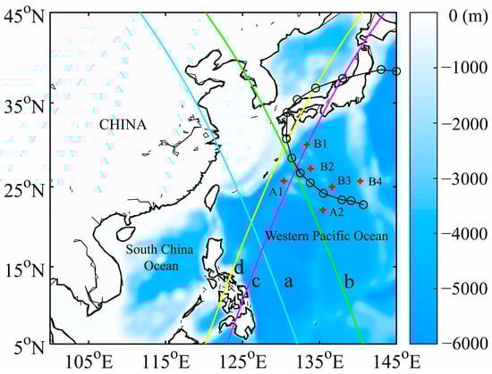
Figure 1.
Bathymetric display of the western Pacific domain and the location information of the data set are presented. The black “−o” line indicates the path of Typhoon Nanmadol, with the typhoon making landfall in Japan from the western Pacific Ocean; the circles along the path represent the position of the typhoon at 12 h intervals. The red “+” markers (A1−B4) denote the locations of the Argo floats; the straight line (a−d) illustrates the Jason-3 altimeter’s trajectory over the western Pacific during the typhoon.
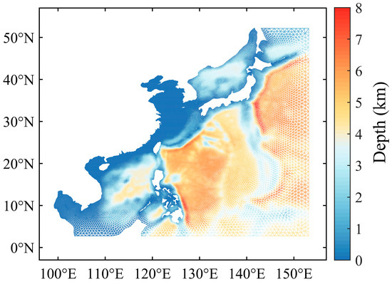
Figure 2.
The western Pacific unstructured grid domain and model water depth information.
The meteorological data are based on a wind-driven model with a resolution of 0.125° × 0.125°, which is obtained every 6 h by ECMWF (https://www.ecmwf.int/, accessed on 1 January 2024). HYCOM data were used as the initial temperature and salinity field (https://www.hycom.org/, accessed on 1 January 2024). Heat flux data of NCEP (https://downloads.psl.noaa.gov/Datasets/ncep.reanalysis/, accessed on 1 January 2024), which are consistent with the precision of the wind field, were used as the source and sink term of temperature change. Optimum Interpolation SST was used to verify sea surface temperatures; NOAA’s 1/4° Daily Optimum interpolated Sea Surface Temperature (OISST) is a long-term climate data record (https://www.ncei.noaa.gov/products/optimum-interpolation-sst, accessed on 1 January 2024). It combines observations from different platforms (satellites, ships, floats) into a regular global grid. AVISO+’ s jason3 satellite altimeter data were used for wave height verification (https://www.aviso.altimetry.fr/en/home.html, accessed on 1 January 2024). The Argo automatic profiling float was used to compare the depth of the mixed layer (http://www.argo.org.cn/, accessed on 1 January 2024).
3.3. Model Setup
The FVCOM-SWAVE, a coupled ocean current and wave prediction model, was utilized for numerical simulation. During the preliminary experimental phase, the wave radiation stress influenced by the geostrophic effect was incorporated into the wave–current interaction module of the model. This means that, in the case of wave fields, the geostrophic effect of the unit mass water body is taken into account in the genesis of ocean currents. In the horizontal direction of the model region, an unstructured triangular grid was used (Figure 2), which consisted of 50,244 units and 26,073 nodes, respectively, with a minimum step size of about 10 km. The open boundary of land, island, and ocean was set in the model, and the dry and wet grid method was used on the coast. Dry points, where the water depth falls below 0.05 m, are defined with zero velocity, and the open boundaries employ a sponge layer to absorb wave energy. The model was vertically divided into 40 layers. The − mixed coordinate was adopted, the coordinate was used for the area with a relatively shallow water depth, and the mixed coordinate was suitable for the area with a relatively deep water depth.
Considering the impact of radiation stress from typhoon conditions on the surface attributes of the upper ocean, both the conventional wave radiation stress scheme and the geostrophic radiation stress scheme were employed to model the surface characteristics’ (wave, flow field, sea surface temperature) responses to these two schemes.
4. Results and Discussion
4.1. Wave Simulation Result
Typhoon Nanmadol generated powerful, typhoon-induced waves. Figure 3 displays four key stages of changes in effective sea surface wave height and influence range due to the significant impact of Typhoon Nanmadol’s wind field. On 15 September (Figure 3a, UTC), Nanmadol transitioned from a tropical cyclone to a typhoon. The central wind speed reached approximately 33 m/s, generating waves about 5.5 m high to the east of its path, with a limited impact on the overall effective wave height. From 16 to 17 September (UTC), as depicted in Figure 3b,c, Nanmadol matured into a super typhoon. The central wind speed peaked at 62 m/s, generating waves about 12 m high in the western Pacific region, with a maximum height of 13.4 m. The area of impact significantly expanded, reaching the East China Sea. On 18 September (UTC), as shown in Figure 3d, Nanmadol developed two eye structures and began the process of eye-wall replacement prior to landfall. This phenomenon, where a strong typhoon replaces a smaller eye with a larger one, is part of its structural adjustment and represents a vulnerable phase during which the typhoon’s intensity typically weakens [49]. Landfall occurred during the critical period of Nanmadol’s eye-wall replacement, which was unsuccessful, leading to the typhoon striking Japan in this vulnerable state. Prior to the typhoon’s landfall, despite the wind field being less intense than at its peak, Nanmadol still generated waves reaching up to 10 m in height on the southern islands of Kyushu.
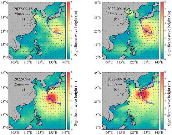
Figure 3.
Significant wave height (Hs) range affected by typhoon wind field; (a–d) stand for 0 o’clock every day from 15 to 18 September.
The effective wave height, as calculated by the FVCOM-SWAVE model, is predominantly influenced by the strength of the wind field, with a secondary influence from the flow field in the lower layers. The primary reason for this is that the horizontal component of the three-dimensional flux increase due to radiation stress from the geostrophic effect is minimal. Furthermore, the two-dimensional flux term remains largely consistent with the original scheme, exerting a negligible impact on wave dynamics, and is therefore often disregarded. The enhanced vertical term magnifies the impact of waves on the subsurface water forces, particularly noticeable in variations in turbulent mixing and sea surface temperature.
To further demonstrate the precision of numerical wave simulations, the effective wave height derived from the Ku-band inversion of the Jason-3 satellite altimeter was utilized to validate the simulated waves. Figure 4a–d illustrate four trajectories observed by satellites during Typhoon Nanmadol. The effective wave heights observed by the satellite were compared with the outcomes of the model simulation.
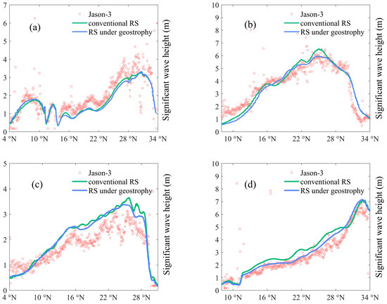
Figure 4.
The numerical simulation results of effective wave height were compared with the Jason-3 satellite altimeter data. (a–d) represent each of the four orbits of the altimeter satellite.
By comparing with satellite altimeter data, it was found that the model can simulate the effective wave height more accurately. The peak error (), correlation coefficient (), mean absolute error (), and root mean square error () were compared to measure the accuracy of wave height simulation results. The specific formula is as follows:
where and , respectively, represent the simulated value and the measured value (inversion value) and and , respectively, represent the average value of the two. The calculated results are shown in Table 1. On the whole, the simulated values of the two RS schemes are close to the satellite altimeter data. The correlation coefficients of three orbits are all above 0.9, the overall mean absolute error () is about 0.3 m, and the root mean square error () is less than 0.6 m. The correlation coefficient between the measured value and the simulated value of orbit a did not reach 0.9, and the peak error () was more than one meter, because the time when the satellite swept orbit a was at the beginning of the numerical simulation, the wave and the wind field in the model were not fully integrated, the average absolute error () was about 0.3 m, and the root mean square error () was less than 0.6 m.

Table 1.
Comparison of ocean wave simulation values with satellite altimeter data.
By comparing the wave results of the two RS schemes, it can be observed that the error under the geostrophic RS effect is slightly smaller than that under the conventional RS scheme. In the context of wave–current interaction, the geostrophic effect RS induces changes in the direction and velocity of ocean currents, resulting in different modulation effects on waves [50]. However, the overall difference between the two schemes is not substantial. Based on the verification of effective wave height, the SWAVE model demonstrates superior capability in simulating the wave processes associated with Typhoon Nanmadol.
4.2. Results of Sea Surface Flow Field
Typhoon Nanmadol escalated into a super typhoon, achieving peak wind speeds of 62 m/s in the western Pacific region. Prior to making landfall in Japan, Typhoon Nanmadol diminished to a strong typhoon due to eye-wall replacement. Its wind speed decreased rapidly upon landfall, reducing its intensity to that of a tropical storm. This section explores the effects of Typhoon Nanmadol on the ocean flow field in the western Pacific before its initial landfall. Figure 5 displays the daily flow fields affected by typhoons throughout the simulation period.
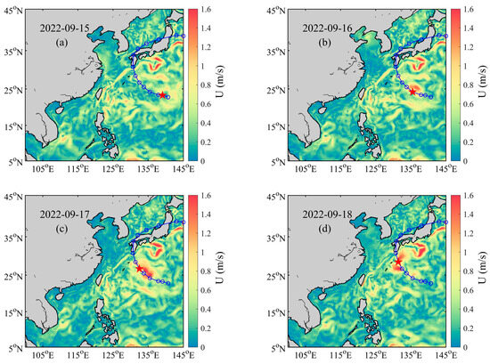
Figure 5.
Numerical simulation of the influence of Typhoon Nanmadol on ocean flow field. (a–d) stand for 0 o’clock every day from 15 to 18 September.
The ocean flow field simulation covered a period from 14 September 2022 (UTC) at 00:00 to 19 September 2022 (UTC) at 00:00, amounting to a total of 5 days. As shown in Figure 5a,b, before 17 September, the flow induced by the typhoon displayed a vortical pattern in the western Pacific Ocean. The flow velocity was lowest at the typhoon’s core, exhibiting a counterclockwise rotation and anticyclonic direction that extended outward. Due to the typhoon’s asymmetrical structure, the flow velocity on the right side, relative to the typhoon’s direction of movement, was greater than that on the left, reaching a peak of 2 m/s. The typhoon progressively moved northward until 18:00 on the 17th (UTC). For instance, as illustrated in Figure 5d, the outer edge of the northern side of the typhoon’s ocean vortex neared the Kuroshio. Concurrently, the typhoon sustained its intensity and the oceanic vortex exhibited robust circulation.
Conventional RS and geostrophic effect RS were utilized to simulate the ocean flow field under Typhoon Nanmadol. Two significant phases were analyzed: 16 September (UTC), when Typhoon Nanmadol evolved into a super typhoon (Figure 6a), and 18 September (UTC), when it reached peak strength (Figure 6b). To provide a clear comparison, the velocity vector fields of the two schemes were overlaid on a graph. Observations revealed minimal differences in the overall flow field intensity between the two simulations, with both generating extensive typhoon-induced vortices. However, in the ocean current divergence regions surrounding the vortices, the divergence amplitude of the surface flow field due to radiation stress within the geostrophic effect was more pronounced, leading to increased velocities. These results indicate that the rightward force of waves induced by geostrophic wave radiation stress under the typhoon field in the northern hemisphere changes the direction of outward divergence of water flow from the vortex center. At the same time, the velocity increases, the turbulent mixing degree of the surface layer of the vortex is enhanced, and the exchange of materials in the upper ocean is intensified, thus causing the temperature of the upper ocean to decrease and the mixing layer to deepen.
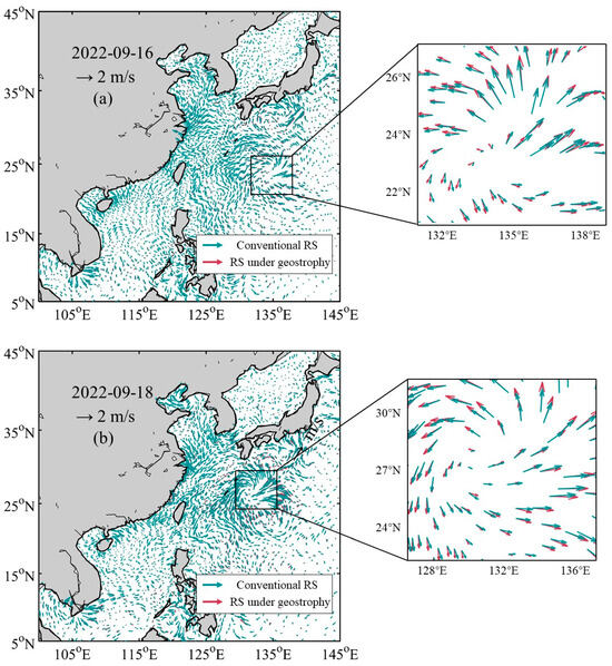
Figure 6.
Comparison of geostrophic effect radiation stress and conventional radiation stress simulated surface flow field vector images in typhoon center. (a,b) refers to the two moments when the typhoon became a super typhoon (48 m/s) and the maximum wind speed (62 m/s) respectively.
4.3. Upper Ocean Temperature Simulation Results
The sea surface temperature (SST) plays a pivotal role as a forcing mechanism between the ocean and the atmosphere, profoundly influencing the formation, path, and strength of typhoons. In turn, the passage of typhoons can significantly modify the SST. Under the influence of a typhoon’s strong wind stress, surface waters within the typhoon’s ocean vortex are pushed away from the center, resulting in seawater divergence and the upwelling of deeper waters. As a result, the SST in the region experiencing the most intense divergence of the typhoon’s ocean vortex becomes noticeably cooler compared to surrounding areas of the vortex [51,52,53].
The sea surface temperature (SST) simulated by the geostrophic effect radiation stress scheme illustrates the overall scenario. The SST on 15 September (UTC) is considered the initial temperature, and the variations in SST across different periods are depicted in Figure 7. Intense mixing and upwelling induced by typhoons result in a decrease in SST. One to two days following the peak typhoon wind speed, the SST experiences the most significant reduction. In the early phase of the typhoon, its strength and the consequent upwelling and divergence are minimal, resulting in a less pronounced decrease in SST. On 17 September at 2:00 UTC (Figure 7c), the typhoon’s central wind speed reached a peak of 62 m/s, coinciding with a substantial decline in SST. The most notable drop in SST occurred on September 18 (Figure 7d, UTC), one day after the maximum wind speed, with temperatures decreasing by approximately 2.5 °C. The reduction in sea surface temperature (SST) propagated from southeast to northwest.
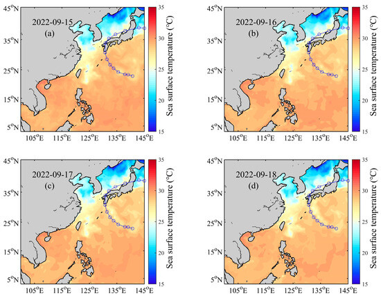
Figure 7.
Sea surface temperature simulation during Nanmadol by radiation stress under geostrophic effect. (a–d) stand for 0 o’clock every day from 15 to 18 September.
From 16 September 2022 (UTC), Typhoon Nanmadol escalated from a strong tropical storm to a typhoon. As the typhoon progressed, the sea surface temperature (SST) in regions experiencing intense seawater divergence along its path exhibited significant cooling compared to neighboring areas, resulting in a distinct cold wake effect. In order to compare the difference in SST caused by the two radiation stress schemes, the SST simulated by the geostrophic effect RS scheme in the whole simulation process was subtracted from the SST simulated by the conventional RS scheme to obtain (°C) (Figure 8). The SST simulated by the geostrophic effect RS in the area with severe typhoon divergence was about 1.0 °C lower than that simulated by the conventional radiation stress scheme. The maximum temperature drop can reach 1.4 °C. The geostrophic effect RS scheme amplifies both the horizontal force and vertical force acting on the water body due to the geostrophic effect component. The water column beneath the sea wave is influenced by the horizontal component of the Coriolis force, while the vertical force at the sea surface also comes into play, enhancing turbulent mixing and consequently leading to a decrease in SST.
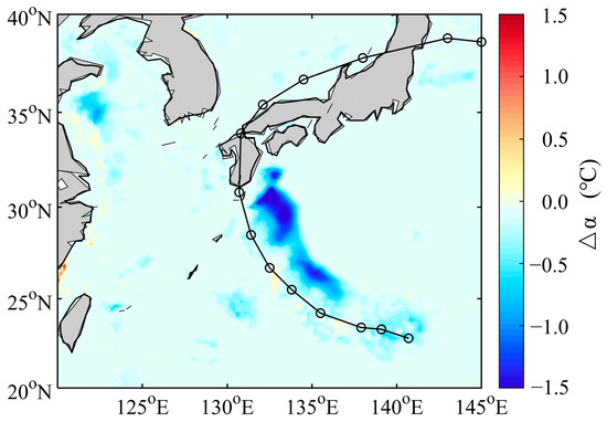
Figure 8.
Numerical simulation of the minimum difference in sea surface temperature between two schemes during Typhoon Nanmadol.
To further verify the accuracy of the Sea Surface Temperature (SST) simulation, the simulated SST was compared with the Optimum Interpolation Sea Surface Temperature (OISST) data (Figure 9a–d). The two-dimensional spatial distribution of the difference between the simulated SST under the geostrophic effect RS scheme and the daily OISST was analyzed. The results indicate that the difference between the simulated and observed SST was less than ±1 °C.
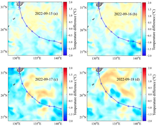
Figure 9.
Comparison of geostrophic effect RS-simulated SST with satellite fusion OISST data. (a–d) stand for 12 o’clock every day from 15 to 18 September.
On 17–18 September (UTC), a significant decline in sea surface temperature was observed due to the influence of the strong wind field associated with Typhoon Nanmadol. Figure 7c,d show cold spots forming in the cooling core area. In Figure 10, the difference between the simulation results of geostrophic effect RS and OISST in the cooling core region is minimal, not exceeding ±0.5 °C. Outside the cooling core area, the model tends to overestimate the sea surface temperature. This discrepancy can be attributed to an overestimation of sensible and latent heat fluxes by the model’s heat flux calculation module [54]. This issue is expected to be addressed in future experiments. Similarly, when comparing the simulation results from both the conventional RS and geostrophic effect RS schemes with the OISST observations (as detailed in Table 2), the correlation coefficient () of SST for the geostrophic effect RS scheme averages at 0.97, indicating an improvement in simulation accuracy. Furthermore, both the mean absolute error () and the root mean square error () were reduced.
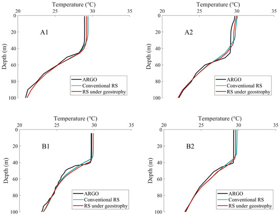
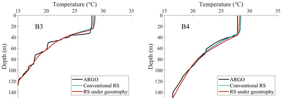
Figure 10.
Comparison of observed sea water temperature and numerical simulation temperature profile with Argo floats; (A1–B4) indicate the locations of the Argo floats.
Table 2.
Comparison of simulated sea surface temperature (SST) with observed values.
To further validate the influence of radiation stress, induced by typhoon conditions, on vertical ocean temperature profiles, Argo floats were employed to contrast the vertical temperature simulations derived from both conventional RS and geostrophic effect RS schemes.
The model’s accuracy was validated by comparing the observed profile temperatures from six Argo floats, positioned along the typhoon’s path, with the simulated profile temperatures. The temperature simulation results from the two RS schemes show minimal differences from the observation results, and both accurately simulate the changes in shallow ocean temperature with depth. The mixing layer depth is determined as the depth at which the temperature decreases by 0.5 °C from the sea surface [55]. Table 3 shows that the observed vertical mixing layer depths from Argo floats are consistently deeper than the simulated values, with an average of around 40 m. The simulated mixing layer depths are generally shallower, ranging from 30 to 40 m, and are on average 2 m less than the observed depths, indicating that the simulated turbulent mixing may be underestimated. To better influence the mixed layer depth, more mechanisms of wave–current interaction should be considered. The differences between the geostrophic effect RS and conventional RS schemes in the simulated profile temperatures are evident in both sea surface temperature and mixed layer depths. When influenced by wave action, the geostrophic effect RS scheme generates vertical shear stress on the subsurface water, calculated as the product of the geostrophic parameter and the Stokes drift velocity. This shear stress enhances the vertical water exchange, leading to the ascent of deeper waters. Consequently, the upper ocean layer cools and the mixing layer deepens, aligning more closely with the observed mixing layer depths.
Table 3.
Comparison between simulated results and observed values of mixed layer depth.
5. Conclusions
We utilized the unstructured grid FVCOM-SWAVE wave and current coupling model to simulate Typhoon Nanmadol in the western Pacific Ocean. This study concentrates on the impact of waves on the ocean flow field, sea surface temperature (SST), and mixed layer depth, especially considering the geostrophic effect RS scheme. Data from the Jason-3 satellite altimeter, Fusion Sea Surface Temperature (OISST) derived from ship measurements, and Argo floats were used to validate the model results and showcase the capability of large-area coupling simulations under extreme wind conditions.
Radiation stress under the geostrophic effect significantly influences ocean dynamics and the distribution of constituents within the upper ocean layers. In contrast to the conventional RS, the geostrophic effect RS scheme extends the radiation stress tensor from two to three dimensions, augmenting the RS components that are affected by the Earth’s angular velocity in both horizontal and vertical directions. This enhancement amplifies the wave influence on water flow during strong typhoons, which subsequently affects the divergence of ocean currents, SST, and the depth of the mixed layer indirectly.
Our analysis indicates that, during the typhoon, the geostrophic effect RS scheme increases surface velocity and induces a rightward deflection compared to the conventional RS scheme. Variations in the surface flow field, induced by geostrophic radiation stress, are closely associated with the distribution of decreased sea surface temperatures.
The enhanced turbulent mixing, resulting from the geostrophic effect radiation stress, leads to a decrease in SST. This underscores the importance of accounting for the geostrophic effect RS when simulating SST, as it results in increased upper ocean mixing and consequently lowers SST. The depth of the mixed layer under typhoon conditions is also examined. While radiation stress primarily affects the surface, the upwelling resulting from upper water body divergence indirectly impacts the entire mixed layer. Under geostrophic effects, this enhances vertical seawater mixing in the deeper layers.
Author Contributions
Conceptualization. J.S.; methodology, X.C. and J.S.; formal analysis, J.S., J.C. and X.C.; writing—original draft preparation, J.C. and X.C.; writing—review and editing, J.S., J.C., J.L., Q.W., Z.Z. and X.C.; Funding acquisition: J.C.; supervision, J.C. and J.S. All authors have read and agreed to the published version of the manuscript.
Funding
This research was funded by the National Key Research and Development Program of China (Grant No. 2021YFB2601100), the National Natural Science Foundation of China (Grant No. 52271257) and the Natural Science Foundation of Hunan Province (Grant No. 2022JJ10047).
Data Availability Statement
The typhoon best track dataset was obtained from the National Weather Service (https://tcdata.typhoon.org.cn/zjljsjj.html, accessed on 1 January 2024). The topographic data were available from NOAA National Centers (http://www.ngdc.noaa.gov/mgg/global/global.html, accessed on 1 January 2024). The wind data can be found in the ECMWF (https://www.ecmwf.int/, accessed on 1 January 2024). The daily averaged heat flux data were provided by the NCEP (https://downloads.psl.noaa.gov/Datasets/ncep.reanalysis/surface_gauss/, accessed on 1 January 2024). The initial temperature field and the salinity field were obtained from the HYCOM (https://www.hycom.org/, accessed on 1 January 2024). The Argo float profile data are available from the International ARGO Program and the national programs (http://www.argo.org.cn, accessed on 1 January 2024). Satellite fusion OISST was used to obtain SST (https://www.ncei.noaa.gov/products/optimum-interpolation-sst, accessed on 1 January 2024). Significant wave height was obtained using the Jason-3 satellite altimeter (https://www.aviso.altimetry.fr/en/home.html, accessed on 1 January 2024).
Acknowledgments
The authors thank the National Weather Service for providing the best track dataset of typhoons, NOAA National Centers for providing the topographic data, ECMWF for providing the wind data, NCEP for providing the daily averaged heat flux data, and the International Argo Program and the National Programs for the Argo float profile data.
Conflicts of Interest
The authors declare no conflicts of interest.
References
- Kumar, V.S.; Harikrishnan, S.; Mandal, S. Wave crest height distribution during the tropical cyclone period. Ocean Eng. 2020, 197, 106899. [Google Scholar] [CrossRef]
- Kumar, V.S.; Anusree, A. High waves measured during tropical cyclones in the coastal waters of India. Ocean Eng. 2023, 289, 116124. [Google Scholar] [CrossRef]
- Liu, G.L.; Yang, W.J.; Jiang, Y.P.; Yin, J.Y.; Tian, Y.H.; Wang, L.P.; Xu, Y. Design Wave Height Estimation under the Influence of Typhoon Frequency, Distance, and Intensity. J. Mar. Sci. Eng. 2023, 11, 18. [Google Scholar] [CrossRef]
- Shen, L.D.; Zou, Z.L.; Zhang, Z.D.; Pan, Y. Exact solution and approximate solution of irregular wave radiation stress for non-breaking wave. Acta Oceanol. Sin. 2021, 40, 58–67. [Google Scholar] [CrossRef]
- Gao, X.; Ma, X.Z.; Li, P.D.; Yuan, F.; Wu, Y.F.; Dong, G.H. Nonlinear analytical solution for radiation stress of higher-order Stokes waves on a flat bottom. Ocean Eng. 2023, 286, 13. [Google Scholar] [CrossRef]
- Longuet-Higgins, M.; Stewart, R. Changes in the form of short gravity waves on long waves and tidal currents. J. Fluid Mech. 1960, 8, 565–583. [Google Scholar] [CrossRef]
- Longuet-Higgins, M.S.; Stewart, R. The changes in amplitude of short gravity waves on steady non-uniform currents. J. Fluid Mech. 1961, 10, 529–549. [Google Scholar] [CrossRef]
- Longuet-Higgins, M.S.; Stewart, R. Radiation stress and mass transport in gravity waves, with application to ‘surf beats’. J. Fluid Mech. 1962, 13, 481–504. [Google Scholar] [CrossRef]
- Longuet-Higgins, M.S.; Stewart, R. Radiation stresses in water waves; a physical discussion, with applications. Deep. Sea Res. Oceanogr. Abstr. 1964, 11, 529–562. [Google Scholar] [CrossRef]
- Longuet-Higgins, M.S. Longshore currents generated by obliquely incident sea waves: 1. J. Geophys. Res. 1970, 75, 6778–6789. [Google Scholar] [CrossRef]
- Noda, E.K. Wave-induced nearshore circulation. J. Geophys. Res. 1974, 79, 4097–4106. [Google Scholar] [CrossRef]
- Bowen, A.J. The generation of longshore currents on a plane beach. J. Mar. Res. 1969, 27, 1153. [Google Scholar]
- Thornton, E.B. Variation of longshore current across the surf zone. In Coastal Engineering 1970; American Society of Civil Engineers: Reston, VA, USA, 2015; pp. 291–308. [Google Scholar]
- Bettess, P. A generalization of the radiation stress tensor. Appl. Math. Model. 1982, 6, 146–150. [Google Scholar] [CrossRef]
- Dolata, L.; Rosenthal, W. Wave setup and wave-induced currents in coastal zones. J. Geophys. Res. Ocean. 1984, 89, 1973–1982. [Google Scholar] [CrossRef]
- Mellor, G. The three-dimensional current and surface wave equations. J. Phys. Oceanogr. 2003, 33, 1978–1989. [Google Scholar] [CrossRef]
- Zheng, J.H.; Yan, Y.X. Vertical variations of wave-induced radiation stress tensor. Acta Oceanol. Sin. 2001, 4, 597–605. [Google Scholar]
- Mellor, G.L. The depth-dependent current and wave interaction equations: A revision. J. Phys. Oceanogr. 2008, 38, 2587–2596. [Google Scholar] [CrossRef]
- Mellor, G. Waves, circulation and vertical dependence. Ocean Dyn. 2013, 63, 447–457. [Google Scholar] [CrossRef]
- Mellor, G. A combined derivation of the integrated and vertically resolved, coupled wave–current equations. J. Phys. Oceanogr. 2015, 45, 1453–1463. [Google Scholar] [CrossRef]
- Ardhuin, F.; Jenkins, A.D.; Belibassakis, K.A. Comments on “The three-dimensional current and surface wave equations”. J. Phys. Oceanogr. 2008, 38, 1340–1350. [Google Scholar] [CrossRef]
- Ardhuin, F.; Rascle, N.; Belibassakis, K.A. Explicit wave-averaged primitive equations using a generalized Lagrangian mean. Ocean Model. 2008, 20, 35–60. [Google Scholar] [CrossRef]
- Ardhuin, F.; Suzuki, N.; McWilliams, J.C.; Aiki, H. Comments on “A combined derivation of the integrated and vertically resolved, coupled wave–current equations”. J. Phys. Oceanogr. 2017, 47, 2377–2385. [Google Scholar] [CrossRef]
- McWilliams, J.C.; Restrepo, J.M.; Lane, E.M. An asymptotic theory for the interaction of waves and currents in coastal waters. J. Fluid Mech. 2004, 511, 135–178. [Google Scholar] [CrossRef]
- Newberger, P.; Allen, J.S. Forcing a three-dimensional, hydrostatic, primitive-equation model for application in the surf zone: 1. Formulation. J. Geophys. Res. Ocean. 2007, 112, C08018. [Google Scholar] [CrossRef]
- Michaud, H.; Marsaleix, P.; Leredde, Y.; Estournel, C.; Bourrin, F.; Lyard, F.; Mayet, C.; Ardhuin, F. Three-dimensional modelling of wave-induced current from the surf zone to the inner shelf. Ocean Sci. 2012, 8, 657–681. [Google Scholar] [CrossRef]
- Craik, A.D.; Leibovich, S. A rational model for Langmuir circulations. J. Fluid Mech. 1976, 73, 401–426. [Google Scholar] [CrossRef]
- Hasselmann, K. Wave-driven inertial oscillations. Geophys. Astrophys. Fluid Dyn. 1970, 1, 463–502. [Google Scholar] [CrossRef]
- Xu, Z.; Bowen, A. Wave-and wind-driven flow in water of finite depth. J. Phys. Oceanogr. 1994, 24, 1850–1866. [Google Scholar] [CrossRef]
- Sun, F.; Qian, C.C.; Wang, W.; Gao, S. Estimation of ocean wave shear force and its convection driving effect. Sci. China 2003, 33, 791–798. [Google Scholar]
- Gao, S.; Sun, F. Analysis of wave-induced lateral body force. J. Oceanol. Limnol. 2005, 36, 367–375. [Google Scholar]
- Sun, F.; Wei, Y.L.; Wu, K.J. Wave-induced radiation stress under geostrophic condition. Acta Oceanol. Sin. 2006, 28, 1–4. [Google Scholar]
- Chen, C.; Liu, H.; Beardsley, R.C. An unstructured grid, finite-volume, three-dimensional, primitive equations ocean model: Application to coastal ocean and estuaries. J. Atmos. Ocean. Technol. 2003, 20, 159–186. [Google Scholar] [CrossRef]
- Niu, Q.; Xia, M.; Rutherford, E.S.; Mason, D.M.; Anderson, E.J.; Schwab, D.J. Investigation of interbasin exchange and interannual variability in L ake E rie using an unstructured-grid hydrodynamic model. J. Geophys. Res. Ocean. 2015, 120, 2212–2232. [Google Scholar] [CrossRef]
- Jiang, L.; Xia, M. Dynamics of the Chesapeake Bay outflow plume: Realistic plume simulation and its seasonal and interannual variability. J. Geophys. Res. Ocean. 2016, 121, 1424–1445. [Google Scholar] [CrossRef]
- Kang, X.; Xia, M.; Pitula, J.S.; Chigbu, P. Dynamics of water and salt exchange at Maryland Coastal Bays. Estuar. Coast. Shelf Sci. 2017, 189, 1–16. [Google Scholar] [CrossRef]
- Chen, J.; Weisberg, R.H.; Liu, Y.; Zheng, L.; Zhu, J. On the momentum balance of Tampa Bay. J. Geophys. Res. Ocean. 2019, 124, 4492–4510. [Google Scholar] [CrossRef]
- Liu, Y.; Weisberg, R.H.; Zheng, L. Impacts of hurricane Irma on the circulation and transport in Florida Bay and the Charlotte Harbor estuary. Estuaries Coasts 2020, 43, 1194–1216. [Google Scholar] [CrossRef]
- Galperin, B.; Kantha, L.; Hassid, S.; Rosati, A. A quasi-equilibrium turbulent energy model for geophysical flows. J. Atmos. Sci. 1988, 45, 55–62. [Google Scholar] [CrossRef]
- Smagorinsky, J. General circulation experiments with the primitive equations: I. The basic experiment. Mon. Weather Rev. 1963, 91, 99–164. [Google Scholar] [CrossRef]
- Qi, J.; Chen, C.; Beardsley, R.C.; Perrie, W.; Cowles, G.W.; Lai, Z. An unstructured-grid finite-volume surface wave model (FVCOM-SWAVE): Implementation, validations and applications. Ocean Model. 2009, 28, 153–166. [Google Scholar] [CrossRef]
- Niu, Q.; Xia, M. Wave climatology of Lake Erie based on an unstructured-grid wave model. Ocean Dyn. 2016, 66, 1271–1284. [Google Scholar] [CrossRef]
- Mao, M.; Xia, M. Dynamics of wave–current–surge interactions in Lake Michigan: A model comparison. Ocean Model. 2017, 110, 1–20. [Google Scholar] [CrossRef]
- Zhang, Y.; Chen, C.; Beardsley, R.C.; Perrie, W.; Gao, G.; Zhang, Y.; Qi, J.; Lin, H. Applications of an unstructured grid surface wave model (FVCOM-SWAVE) to the Arctic Ocean: The interaction between ocean waves and sea ice. Ocean Model. 2020, 145, 101532. [Google Scholar] [CrossRef]
- Mellor, G.L.; Yamada, T. Development of a turbulence closure model for geophysical fluid problems. Rev. Geophys. 1982, 20, 851–875. [Google Scholar] [CrossRef]
- Svendsen, I.A. Mass flux and undertow in a surf zone. Coast. Eng. 1984, 8, 347–365. [Google Scholar] [CrossRef]
- Wu, L.; Chen, C.; Guo, P.; Shi, M.; Qi, J.; Ge, J. A FVCOM-based unstructured grid wave, current, sediment transport model, I. Model description and validation. J. Ocean Univ. China 2011, 10, 1–8. [Google Scholar] [CrossRef]
- Moghimi, S.; Klingbeil, K.; Gräwe, U.; Burchard, H. A direct comparison of a depth-dependent radiation stress formulation and a vortex force formulation within a three-dimensional coastal ocean model. Ocean Model. 2013, 70, 132–144. [Google Scholar] [CrossRef]
- Wu, Z.H.; Zhang, Y.; Zhang, L.F.; Zheng, H.P. Interaction of Cloud Dynamics and Microphysics During the Rapid Intensification of Super-Typhoon Nanmadol (2022) Based on Multi-Satellite Observations. Geophys. Res. Lett. 2023, 50, 9. [Google Scholar] [CrossRef]
- Sun, Y.; Perrie, W.; Toulany, B. Simulation of wave-current interactions under hurricane conditions using an unstructured grid model: Impacts on ocean waves. J. Geo-Phys. Res. Ocean. 2018, 123, 3739–3760. [Google Scholar] [CrossRef]
- Zhang, J.S.; Lin, Y.L.; Chavas, D.R.; Mei, W. Tropical Cyclone Cold Wake Size and Its Applications to Power Dissipation and Ocean Heat Uptake Estimates. Geophys. Res. Lett. 2019, 46, 10177–10185. [Google Scholar] [CrossRef]
- Da, N.D.; Foltz, G.R.; Balaguru, K. Observed Global Increases in Tropical Cyclone-Induced Ocean Cooling and Primary Production. Geophys. Res. Lett. 2021, 48, 8. [Google Scholar] [CrossRef]
- Sun, Z.; Shao, W.; Yu, W.; Li, J. A study of wave-induced effects on sea surface temperature simulations during typhoon events. J. Mar. Sci. Eng. 2021, 9, 622. [Google Scholar] [CrossRef]
- Chen, C.; Beardsley, R.; Hu, S.; Xu, Q.; Lin, H. Using MM5 to hindcast the ocean surface forcing fields over the Gulf of Maine and Georges Bank region. J. Atmos. Ocean. Technol. 2005, 22, 131–145. [Google Scholar] [CrossRef]
- Holte, J.; Talley, L.D.; Gilson, J.; Roemmich, D. An Argo mixed layer climatology and database. Geophys. Res. Lett. 2017, 44, 5618–5626. [Google Scholar] [CrossRef]


Disclaimer/Publisher’s Note: The statements, opinions and data contained in all publications are solely those of the individual author(s) and contributor(s) and not of MDPI and/or the editor(s). MDPI and/or the editor(s) disclaim responsibility for any injury to people or property resulting from any ideas, methods, instructions or products referred to in the content. |
© 2024 by the authors. Licensee MDPI, Basel, Switzerland. This article is an open access article distributed under the terms and conditions of the Creative Commons Attribution (CC BY) license (https://creativecommons.org/licenses/by/4.0/).