Abstract
In order to meet the high uniformity calibration requirements for scientific-grade, large-size space detectors used in the CHES Extrasolar Planet Exploration Mission, this paper presents the design of a wide dynamic range, high uniformity spectral irradiance source (WHUIS). Utilizing a cascade integrating sphere design, and optimizing the overlapping area radiant flux adjustment structure and illumination light path, we achieve a wide dynamic range and high uniformity irradiance output. We established an irradiance transmission model based on the new assumption and analyzed the influence of factors such as illumination distance, stray light, and non-uniform radiance on the uniformity of irradiance output. The model is then validated by building experimental equipment. The findings show that in a circular area of 40 mm, the irradiance uniformity of our light source system exceeds 99.9%, and constant color temperature is adjustable within six orders of magnitude, consistent with the uniformity level predicted by the model.
1. Introduction
The exploration of extrasolar planets is crucial to our understanding of the universe’s mysteries and offers significant insights into the origins and evolution of life. A standout among these explorations is the Closeby Habitable Exoplanet Survey (CHES) mission, a space-based project dedicated to the high-precision optical measurement and detection of extrasolar planetary systems. This mission extensively and accurately investigates planetary systems, specifically focusing on terrestrial planets situated within habitable zones [1]. The core scientific instrument carried in the CHES mission is a telescope. The response uniformity of the scientific-grade large-size detector in the camera component is an important performance parameter for micro-pixel star spacing measurements in the key technology of the CHES [2].
Therefore, the current challenge requires creating a large-scale irradiance field with a high level of uniformity and a wide dynamic range, quantitatively describing the radiant flux received by each pixel and correcting for the uniformity of the detector’s response non-uniformity. Currently, there are many ways to create such an irradiance field, such as beam shaping based on free-form mirrors [3], the application of high-power LED modules [4], and star point plate illumination [5]. These illumination methods can provide high-power irradiance output within a range of about 100 mm × 100 mm, but the uniformity attainable is generally limited to around 99%.
The integrating sphere (IS) light source has a better level of uniformity than these methods. Given the low light conditions encountered by space detectors, the irradiance output range of the IS light source is congruent with the requirements. Therefore, the IS light source is often chosen as the calibration light source for the space detector. For example, the National Metrology Institute of Japan (NMIJ, Tsukuba, Japan) reported that a sintered PTFE IS with a diameter of 84 mm achieved a uniformity of 99.864% in an area of 6 mm × 6 mm [6]. The Physikalisch-Technische Bundesanstalt (PTB, Berlin, Germany) uses a conventional device based on a lamp monochromator, which can achieve a 99.6% spatial uniformity over a 5 mm diameter aperture [7]. The National Institute of Standards and Technology (NIST, Gaithersburg, MD, USA) achieved 99.97% spatial uniformity on a 5 mm diameter aperture at the output of a 300 mm diameter IS light source using a high-power wavelength tunable laser [8]. These studies have achieved a high level of uniformity, but there is still a need to extend the irradiance field for practical applications in the space detector.
In addition, the adjustment of the wide dynamic range is also crucial for the calibration test of the detector, although there have been studies to achieve the expansion of the dynamic range through technologies such as the multi-sub IS light source [9] and the wedge-shaped gradient diaphragm [10]. However, the dynamic range of its adjustment is only about four orders of magnitude. To broaden the dynamic range of radiation output, the triple IS light source developed by L. Yongqiang expands the dynamic range of output radiation to seven orders of magnitude by switching between high and low light channels and a variable aperture [11]. However, the uniformity level is below 99%, and the constant color temperature output cannot be achieved.
In order to address this challenge, this paper develops a wide dynamic range, high uniformity spectral irradiance source (WHUIS). In Section 2, the component structure of the WHUIS system and the functional roles of each part are introduced first. Subsequently, the principle of the light source system is introduced, and then the structural design principle of the three components, namely, the cascade integrating sphere, the diaphragm module, and the illumination path, is described in detail. Furthermore, the design parameters of the WHUIS are provided. In the Section 3, an irradiance transfer model of the WHUIS is proposed, and the characteristic parameters and design parameters in the model are analyzed. The optimized values of the design parameters are obtained from the model. In Section 4, a specialized experimental apparatus is constructed for the purpose of measuring the uniformity and dynamic range of WHUIS output, determining the performance of the light source system, and validating the reasonableness of the model. In Section 5, a comprehensive overview of the work presented in this study is provided, along with an outline of potential avenues for future research and applications.
2. Principle and Design
The objective of the wide dynamic range, high uniformity spectral irradiance source (WHUIS) is to achieve high uniformity and wide dynamic irradiance output adjustment. As illustrated in Figure 1, the system is divided into two distinct components: the precision control system and the optical system. The primary objective of the precision control system is to regulate the output characteristics of the light source with precision, through the adjustment of the tungsten halogen lamp current, the control of the diaphragm module aperture size, and the monitoring of the detector signal to the host computer in real-time.
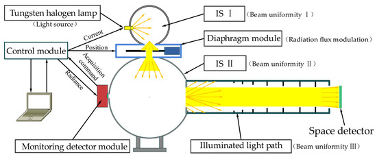
Figure 1.
Schematic diagram of the WHUIS system components.
The optical system consists of three parts: a cascade integrating sphere, a diaphragm module, and an illumination light path. The initial beam is emitted by a tungsten halogen lamp and enters the integrating sphere I (IS I) for preliminary light uniformity; after adjustment by the diaphragm module, the beam enters the integrating sphere II (IS II) for secondary uniformity. After the final transmission and adjustment of the illumination light path, based on the irradiance transmission principle, the beam achieves the third uniformity improvement at the outlet. This results in a high uniformity level irradiance output in the circular area at the light source outlet, which is suitable for detector calibration.
2.1. Principle of the Light Source System
The integrating sphere (IS) is a uniform light source commonly used to calibrate optical instruments. The light undergoes multiple diffuse reflections within the inner cavity and finally emerges as a uniform light beam at the light outlet [12]. The cascade integrating sphere comprises two integrating spheres, including a primary integrating sphere (IS I) and a secondary integrating sphere (IS II), and an adjustable diaphragm module. After two rounds of beam uniformity, the radiance LS of the IS II light outlet can be expressed as follows:
In Equation (1), ρ is the diffuse reflectance of the inner surface; the parameter f = (Ai + Ao)/Ais is the opening ratio of the integrating sphere; Ais is the area of the inner surface; Ai is the area sum of the light inlet; Ao is the area sum of the light outlet; η1 is the energy conversion efficiency of the IS I, which is the ratio of the output radiant flux Φo of the primary IS to the input radiant flux Φi; and η2 is the energy conversion efficiency of the diaphragm module, which is the product of the loss constant H and the aperture adjustment coefficient T(l).
In comparison to a single IS, a cascade IS allows the process of light uniformity to be performed twice, thereby significantly improving the uniformity, which is typically reaches or exceeds 99.5%. The diaphragm module ensures that the beam’s uniformity, color temperature, and polarization state are maintained throughout flux adjustments.
Figure 2 illustrates the principle of radiant flux adjustment. The left square is the aperture of the blocking diaphragm, and the right square is the aperture of the light outlet of the diaphragm module. Their diagonal lengths are J1 and J2, respectively. The servo motor drives the blocking diaphragm to move so that the two apertures produce an overlap area as shown in the yellow shaded area in Figure 2. By changing the overlap area, the radiant flux transported from the IS I to the IS II is controlled. The advantage is that a wide range of constant color temperature adjustments can be achieved while the current of the tungsten halogen lamp remains unchanged. It has higher repeatability and accuracy, which is more conducive to repeated measurements and precise calibration.
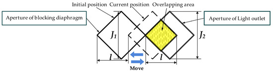
Figure 2.
Principle diagram of radiant flux adjustment.
The ratio of the overlap area SA to the pedestal aperture area S is the adjustment coefficient T(l), which is expressed as follows:
In Equation (2), n is the number of steps the motor moves, and lmin is the minimum step distance of the motor.
Subsequently, the light beam emitted from the diaphragm module passes through the uniform light of the IS II and is then output into the illumination light path. As shown in Figure 3, the illumination light path is a circular diaphragm tube with apertures. According to relevant theories [13], the conversion factor K from irradiance to radiance of the cylindrical diaphragm in the illumination light path can be obtained using the length z of the cylindrical diaphragm tube, the radius a of the inlet aperture, and the radius b of the outlet aperture as follows:
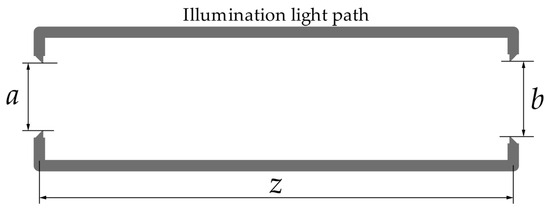
Figure 3.
Schematic diagram of the illumination light path conversion coefficient K.
To simplify the result, set three new variables as follows:
The illumination factor F in Equation (3) is expressed as follows:
Based on the above equations, it can be obtained that the irradiance output E of the WHUIS light source system outlet under ideal conditions is expressed as follows:
2.2. Design of the Light Source System
2.2.1. Cascade IS Design
First, the diameter d required to establish a circular uniform irradiation field based on the effective size of the detector is determined. Based on the estimated irradiance calculated using Equation (6) and laboratory measurement experience, ensure that the irradiance is within the CHES calibration range (10−4~102 μW/cm2) to obtain the appropriate IS II light outlet diameter D.
Then taking D as input, derive the parameters inside the cascade IS. Considering the high uniformity requirements of the CHES mission, focus on improving the uniformity value. The IS maintains a diameter ratio of approximately 1:3 [14]. The diameter ratio is defined as the ratio of the IS’s light outlet to its inner diameter, expressed as D/D2 and DC/D1, respectively. It can be demonstrated that the diameter ratio of the IS has a direct impact on the uniformity of the output beam. Nevertheless, it should be noted that a ratio of D1/D2 greater than 1:3 may affect the energy transmission efficiency.
The aperture of the blocking diaphragm selects the middle part of the beam emitted from the IS for output, which can reduce the impact of reflection and scattering inside the diaphragm module on the uniformity of the output beam. Consequently, the light outlet J2 of the diaphragm module needs to be slightly smaller than the IS I light outlet DC. In addition to considering that the total area of the opening of the IS hole is generally less than 5% of the total inner surface area [15], the thickness of the coating and the shell sphere are important factors, and the IS II light inlet hole is a realistic port [16]. Therefore, the light inlet hole dP of the IS II must be larger than J2 to reduce the reflection of the beam in it and improve the uniformity of the IS II beam.
The smaller the pinch angle is, the better the uniformity of the IS output. However, the larger the angle is, the higher the irradiance of the integrating sphere outlet, and there is a difference of about 9.5% between the irradiance of the 90° angle and the 10° angle. It should be noted that the uniformity gain of narrowing the angle is not as large as the gain of increasing the improved radiance because the uniformity gain depends mainly on the effect of the illumination light path. Therefore, a 90° angle (L-shape) was adopted in the design, which is the optimal choice for the trade-off [17]. The designed structural parameters are shown in Figure 4.
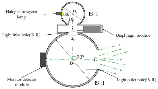
Figure 4.
Structural design diagram of the cascade integrating spheres.
2.2.2. Diaphragm Module Design
Figure 5 shows an expanded view of the structural design of the diaphragm module, in which the cover plate is connected to IS I and the pedestal is connected to IS II. The servo motor is installed on a precision-machined plane, and both ends of the blocking diaphragm are fixed on high-precision ball slide rails. The push rod of the linear motor drives the blocking diaphragm to move forward and backward on the slide rails.
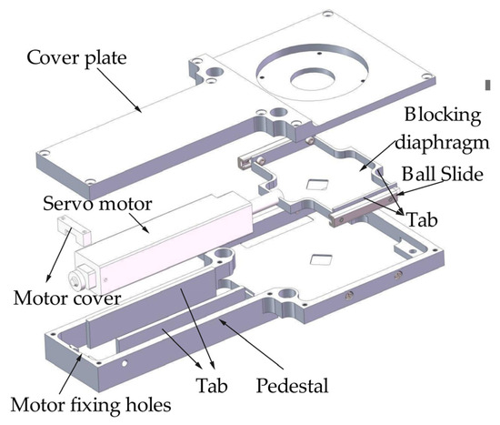
Figure 5.
Structural design diagram of the diaphragm module.
There are two ways to achieve a wide dynamic range. One is to increase the upper limit of the light source output power, and the other is to lower the lower limit of the light source output. Increasing the power will be limited by the heat dissipation power, so reducing the output lower limit of the light source is the key to broadening the output range.
There are two ways to reduce the output lower limit. One is the radiant flux adjustment mechanism. The reason for choosing the square hole to move in the diagonal direction is that the adjustment coefficient T(l) is a quadratic value. Thus, when the l value is small, the adjustment coefficient can obtain a very small value, thereby reducing the lower limit of the radiant flux and achieving a larger dynamic range.
There is another way is to reduce light leakage when the blocking diaphragm is closed. Light leakage is the phenomenon of light escaping from the aperture when it is closed, which will cause the lower limit of the radiant flux to increase. To reduce light leakage, the propagation path and outlet can be blocked together.
As shown in Figure 6a, the distance dg between the tab and the cover plate, the distance db between the blocking diaphragm and the pedestal, and the distance dh between the blocking diaphragm and the cover plate can be reduced on the path to compress the space size of the propagation path. Thus, the rays need to be reflected multiple times to reach the light outlet so that the leaked light will be absorbed in multiple reflections.
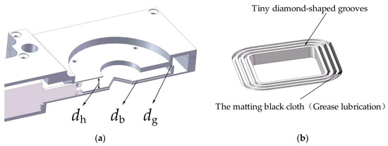
Figure 6.
Detailed view of the diaphragm module. (a) Structural design diagram of distance in the diaphragm module; (b) Structural design diagram of the light trap.
In addition, as shown in Figure 6b, a light trap is set at the outlet, and three tiny diamond-shaped grooves are machined on the edge of the pedestal aperture hole and filled with matte black cloth. The matte black cloth and the blocking diaphragm are closely attached and lubricated with grease during the stroke to prevent light from escaping. Finally, the diaphragm module is internally coated with Avian Black-S, which has a reflectivity of less than 4%. Using these comprehensive measures, the light leakage level is reduced to one-millionth of that in the fully open state.
2.2.3. Illumination Light Path Structure Design
The illumination light path (ILP) is the propagation path between the IS and the detector. In order to reduce external stray light interference, the ILP is closed. However, due to the diffuse light emitted from the light outlet of the IS at a large angle, stray light will be generated through reflection and scattering in the ILP. When designing the ILP, it is necessary to reduce stray light as much as possible so that it can spread in free space close to ideal conditions and ensure high uniformity of light source output.
The structural design of the ILP is shown in Figure 7, which consists of baffles and vanes. Baffles and vanes are often used to block low-order stray light paths and are the main means of dealing with stray light in optical systems [18]. Baffles are usually cylindrical tubes used to closed systems or block zero-order stray light. Vanes are structures used to block baffle scattering. The primary mirror of the classic Cassegrain telescope uses baffles and vanes as the main means of eliminating stray light. In this paper, the stray light generated by the large-angle light emitted from the light outlet of the IS can also be eliminated by referring to the structure, but some additional specific designs are required.
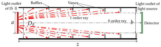
Figure 7.
Structural design diagram of the illumination light path.
First, determine the size DB of the baffle, and set it to double the light outlet diameter of the IS. Then, as shown in Figure 6, design the position and size of the vanes according to the standard of blocking all first-order stray light [19] to prevent the detector from seeing the part of the inner wall of the baffle that is both a critical surface and an illumination surface. At this time, only a small amount of high-order stray light remains in the stray light in the ILP.
Second, it is necessary to pay attention to the design such that the number of baffles should not be too many, especially in the part close to the light outlet of the IS; otherwise, the luminous flux scattered by the edge of the blade will be greater than that without the vanes. In this article, the design parameters of the vanes are adjusted. The vanes close to the light outlet of the IS have moved farther away, and the first vane is canceled.
Third, the angle of the vanes edge slope should be determined to ensure that it is not the critical surface and the illumination surface at the same time. The vanes on the side close to the light outlet of the IS need to face the light outlet of the IS so that it will not become a critical surface. The vanes on the side close to the outlet of the ILP need to face the outlet side so that it will not become the illuminated surface. The design can increase the angle between the scattered light first reflected in the high-order stray light path reaching the detector and the specular reflected light, thereby reducing BRDF and reducing the luminous flux of stray light. For numerical values, please refer to [20].
Last but not least, a fine thread structure needs to be made on the inner wall of the baffle and painted with highly absorbent Avian Black-S black paint to reduce internally reflected stray light by increasing the efficiency of absorbing light. It is worth noting that the traditional blackening process will produce more stray light due to its lower absorption rate. After experimental testing, the uniformity with the traditional blackening process will be reduced to less than 99%, so it cannot be used as a coating inside the ILP.
The finalization of these parameters requires the establishment of a specific mathematical model and the determination of reasonable design values through simulation.
Finally, the designed parameters of the WHUIS, as shown in Table 1, are presented. The optimization of the design parameters will be employed within the simulation model.

Table 1.
Design parameters of the WHUIS.
3. Irradiance Transfer Simulation and Parameter Optimization
In general, the use of ray tracing software such as TracePro7.4.3 and LightTools8.4.0 is suitable for situations where the uniformity of the irradiance transfer of the IS is below 99%. The primary reason for the inability to simulate high uniformity ISs is the lack of knowledge regarding the BRDF model of the IS coating and the substantial statistical noise generated by Monte Carlo random rays in optical simulations [21]. The secondary reason is that the process requires millions of ray tracings, which is time-consuming. Consequently, for the transfer process of a highly uniform IS in a closed cavity (ILP), it is more appropriate to establish a mathematical model and then perform a numerical simulation.
3.1. Irradiance Transfer Model
As illustrated in Figure 8, the irradiance transfer in the ILP is based on the classical radiative transfer theory [22]. This process can be viewed as the cumulative irradiance of countless tiny luminous points on the surface of the IS’s light outlet, which is then received by one receiving point on the detector. The integral method can be employed to calculate the cumulative irradiance, which allows the irradiance E (x2, y2, φ1, φ2) of a specific receiving point on the detector to be obtained as follows:
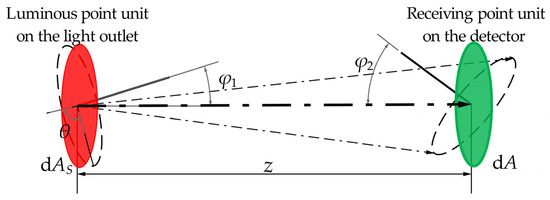
Figure 8.
Principle diagram of irradiance transfer from the luminous point unit to the receiving point unit.
Although Equation (3) can accurately simulate the irradiance of each receiving point on the detector, in actual simulations, the number of light outlet units is always constrained. As illustrated in Figure 9, by partitioning the light outlet into a finite number of luminous point units (red grids), the irradiance contribution of each luminous point unit to the receiving point unit (yellow grid) on the detector is calculated discretely. This allows the irradiance distribution information on the detector to be obtained as follows:
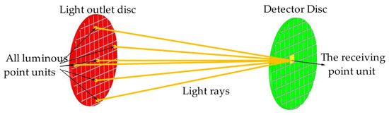
Figure 9.
Principle diagram of discretized irradiance transfer from the light outlet to the detector.
In Equation (8), Ns is the number of finite units, which determines the approximation accuracy of discretization, and Ad is the area of the luminous point unit.
The number of units of a finite element is inversely related to the size of the unit of the finite element on a plane of fixed area. The smaller the area of the units of the finite element is, the closer it comes to the concept of infinitesimal points, i.e., the higher the accuracy. Considering both the computation time and the accuracy in uniformity, the trade-off is to choose a unit of 401 × 401, and this choice will satisfy the model’s resolution requirements.
In the Lambertian model, the radiance LS in Equation (8) is regarded as a constant, which is considered to be at different positions (x,y) and directions (φ,θ). All other variables remain constant. The Lambertian model is the most commonly used theory in IS irradiance simulation. Nevertheless, there are certain limitations, particularly in the overestimation of the symmetry and uniformity of the irradiance distribution.
In actual experiments, the radiance of the IS is observed to exhibit asymmetry in position (x,y) and direction (φ,θ). When measuring the uniformity of the illuminated surface of the IS, the standard measurement procedure is to fix the measurement direction, such as setting (φ,θ) to zero or a certain constant. This simplifies the measurement procedure. This requires the normal position of the detector to be aligned with the light outlet, followed by the measurement of the irradiance by changing the position of the detector (x2, y2).
In order to more accurately reflect the actual irradiance of the IS light source, this paper proposes a new hypothesis: the radiance LS of the light outlet is independent of the direction (φ,θ) and only related to the position (x,y). This hypothesis is termed the asymmetry hypothesis and is more aligned with practical measurement operations, can more accurately simulate and evaluate the actual irradiance distribution and provides a more reasonable theoretical basis for optimizing the design of the IS.
In the Asymmetry model, the consideration of direction (φ,θ) is removed, resulting in the irradiance at the light outlet being proportional to the radiance value. The design and structure of the IS ensure that its radiance reaches its maximum value at a specific location without multiple peaks. Consequently, the hypothesis implies that we determine that there is a point (referred to as point N) at which the radiance reaches the maximum; at the same time, it is necessary to ensure that the overall uniformity of the radiance reaches the specified standard. In the hypothesis, the distribution of radiance is not considered to fluctuate randomly but rather is described as a mountain-like surface, with point N located at the top of the mountain. The change in radiance from point N to the edge can be expressed using a linear equation. Consequently, it can be postulated that the radiance value LS at a specific point on the light outlet of the IS is expressed as follows:
In Equation (9), LMAX represents the strongest radiance, which is obtained at point N (xmax,ymax); Lmin represents the lowest radiance, which is obtained at point V(xmin,ymin); pA represents the distance between a certain point(x1,y1) and point N; and dA represents the distance between point N and point V on the surface of the light outlet.
It is also pertinent to note that in practical settings, optical systems are frequently situated within enclosed spaces, such as diaphragm-shaped darkrooms, where the introduction of stray light can have a detrimental impact on the uniformity of the output.
The stray light matrix is designed to quantitatively model the effect of stray light on the irradiance E at each position (x2,y2) on the detector plane. The light that produces this effect consists of unextinguished low-order stray light as well as higher-order stray light. For each position (x2,y2) on the detector, there exists a corresponding stray light coefficient KS(x2,y2), so the detector plane corresponds to a stray light matrix DK. The distribution of KS on the detector plane is actually quite complex, but there is a general trend of a strong center and bottom edge, and the change in this trend is smooth.
Since the detector plane is circular, it is a rotationally symmetric figure. To simplify the mathematical form of the stray light matrix, the distribution of the stray light coefficients, KS, on the detector plane is expressed as the normalized value of a quadratic function, F(p). p is the optical axis offset distance, p = x2 + y2. The maximum value of this quadratic function, n (normalized value) is obtained at the detector center (0,0), and the minimum value, m, is obtained at the detector edge (x2 + y2 = 202). To determine the stray light ratio m/n, one can determine the quadratic function F(r), the quadratic term coefficient a1 = (m − n)/r2, and the constant term for b1 = n. The stray light coefficient, KS, can be calculated as follows:
Additionally, the stray light coefficient matrix DK is provided with a value of m/n to 1, which decreases with increasing p. Multiplying the stray light coefficients KS by the original irradiance E0(x2,y2), we obtain the irradiance E(x2,y2) after being affected by the stray light:
Equation (11) comprehensively considers the asymmetric distribution of radiance at the light outlet, the uniformity level of radiance, and the joint impact of stray light on the results during the irradiance transfer process. Compared with the Lambertian model, it is more closely aligned with actual conditions.
3.2. Analysis of Irradiance Transfer Simulation
When evaluating the uniformity of the irradiance distribution of the radiation received by a detector, the coefficient of variation (i.e., the ratio of the standard deviation to the mean) is the most commonly used evaluation method.
In Equation (12), Ei represents the irradiance value of each receiving point, while Emean denotes the average irradiance of all receiving points.
Another crucial parameter is the relative distance rxd, which is defined as follows:
In Equation (12), D represents the diameter of the light outlet. The relative distance rxd is the effective distance between the IS light outlet and the detector. Typically, as illustrated in Figure 10, an IS conducts calibration tests in a near-field area. Some studies have proposed that the optimal distance for IS calibration tests is rxd = 5, which is also known as the “five-times rule” [23]. The EMVA 1288 Sensor and Camera Calibration Standard Guide recommends that irradiance uniformity can reach 99.5% when the relative distance from rxd reaches 8 [24]. When the rxd is set to a value greater than 10, it is possible to achieve a higher level of uniformity in the irradiance field, thus meeting the calibration requirements of the spatial matrix detector.
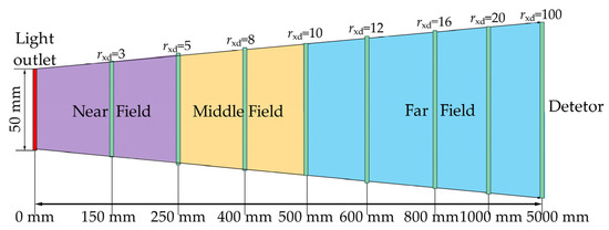
Figure 10.
Principle diagram of relative distance.
The Asymmetry model comprises multiple input parameters, including radiance ratio (Lmin/Lmax), radiance peak position N (xmax,ymax), stray light ratio (n/m), distance z, the diameter of the light outlet of the IS D, and detector radius r. Among these, the radiance ratio (RR) and stray light ratio (SLR) are characteristic parameters of the model itself, which must be obtained through relevant experience and experimental data. The remaining parameters are design variables, and the predicted values can be obtained through the application of principles and experience. The optimized values of the predicted values can then be obtained using the model.
The initial step is to investigate the impact of specific parameters on the uniformity of the model. The aforementioned design parameters should be utilized as the preset values, with the RR represented on the X-axis and the SLR on the Y-axis. The uniformity value obtained by the model should be represented on the Z-axis. A three-dimensional surface diagram of the uniformity value under the change of the two characteristic parameters is presented in Figure 11.
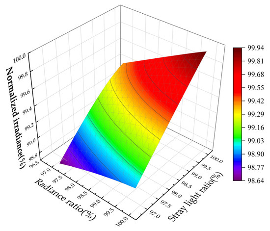
Figure 11.
Three-dimensional surface plot of the uniformity level under changes in the radiance ratio and the stray light ratio.
Figure 11 illustrates that, in the positive direction of the X-axis and Y-axis, the uniformity is rising, with the rising speeds of the two differing. It can be observed that the rate of the increase in the Y-axis is greater than that of the X-axis, indicating that SLR contributes more to the uniformity. Upon examination of the three-dimensional graph, it becomes evident that when both the RR and the SLR reach maximum values, the uniformity ratio attains a maximum value. The maximum value represents the result of the Lambertian model. Consequently, an Asymmetry model has been developed on the Lambertian model, incorporating disturbance factors related to characteristic parameters.
In order to more clearly express the influence of characteristic parameters on uniformity, the radiance ratio is fixed at 99.9%, while the SLR is varied from 99.7% to 99.9% to obtain the uniformity curve. Subsequently, the two parameters are exchanged to obtain a second uniformity curve, which is then plotted alongside the first curve in Figure 12.
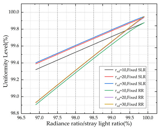
Figure 12.
The uniformity level curves of the fixed radiance ratio (RR) and stray light ratio (SLR).
The uniformity change curve when both RR and SLR are fixed is depicted in Figure 12. It can be demonstrated that the characteristic parameter is proportional to the uniformity. It can be observed that the three straight lines for a fixed SLR are above the curve for the fixed RR, and A higher rxd will make the curve sit higher. It is noteworthy that when RR is fixed, the distance between the straight lines representing different rxd is greater than when SLR is fixed. Furthermore, the difference between rxd = 20 and rxd = 30 is minimal. It can therefore be concluded that in the Asymmetry model, the RR is more responsive to the enhancement of relative distance than the SLR in improving uniformity. Furthermore, an increase in the rxd (rxd ≥ 20) has little impact on the improvement in uniformity.
The determination of characteristic parameters necessitates experimental data and relevant research experience [25,26]. It can be seen that in the case of the SLR, the determination of this characteristic parameter is contingent upon the efficacy of stray light cancellation. It is therefore evident that only a well-designed stray light system can achieve a high value for the SLR. The experimental results in the approximate free propagation case were obtained by testing in a large dark room and then compared with the experimental results of the illuminated light path to obtain a range of values for the stray light ratio, which was taken as 99.9% here. Regarding the determination of RR, a value of 99.8% was derived from relevant research results and experience.
3.3. Discussion and Parameter Optimization of the Irradiance Transfer Model
Once the characteristic parameters had been determined, optimization was carried out for the initial pre-design of the outlet diameter D and the detector diameter d. As previously noted, D was fixed, and the uniformity variation curve with d from 40 to 60 was plotted. Once again, the value of d is fixed, and a uniformity curve is plotted as the value of D changes from 40 to 60. The two curves are presented in Figure 13, with the former represented by a solid line and the latter by a dotted line.
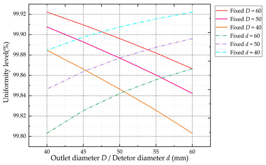
Figure 13.
The uniformity level curves of the fixed outlet diameter and the detector diameter.
Figure 13 illustrates a positive correlation between D and uniformity, while d exhibits an inverse correlation. In order to achieve the CHES uniformity target of 99.8%, a margin is required. Consequently, the uniformity target is set at 99.9% in the design. In Figure 13, three curves are identified that meet this requirement: fixed D = 60, D = 50, and d = 40 with d < 42.5, d < 48, and D > 46, respectively. Furthermore, it is important to note that an increase in D will result in an increase in the size of the light source. Thus, the optimal values for D and d were determined to be 50 mm and 40 mm, respectively, based on the model optimization and practical experience. Given that the diaphragm inlet aperture size in the illumination light path is the outlet size D, it follows that a = 50 mm. To prevent vignetting and blocking and simultaneously avoid the introduction of external stray light, the aperture of the outlet diaphragm must be larger than the detector’s d value. This value is b = 52 mm.
Once the parameter above has been identified, it is possible to compare the simulation results of the Asymmetry model and the Lambertian model. Figure 13 illustrates the uniformity change curve, calculated based on the Lambertian model and the Asymmetry model, within the circular plane area of the 40 mm detector.
As illustrated in Figure 14, the uniformity curve of the Lambertian model consistently exhibits values above 99.9%. When rxd = 30, the uniformity reaches 99.99%. In the context of the Asymmetry model, the fluctuation of the uniformity value within the interval is a consequence of the consideration of the change in the radiance peak point N (xmax, ymax). From rxd = 12 onwards, the uniformity of the central area (0, 0) begins to exceed that of the edge area (x2 + y2 = 202). As rxd increases, the difference between the two areas becomes more significant. The uniformity data for different rxd values can be found in Table 2. When rxd = 20, the uniformity under the Asymmetry model ranges from 99.909% to 99.921%.
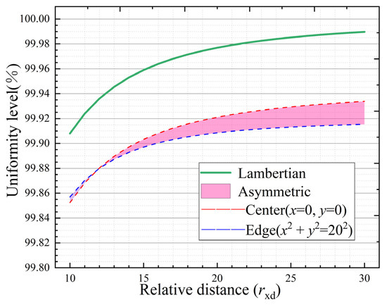
Figure 14.
The uniformity curves of the Asymmetry model and the Lambertian model change with relative distance.
Table 2.
Evaluation values of uniformity for the simulation on the Lambertian model and Asymmetry model.
It is evident that, in contrast to the Lambertian model, the increase in rxd(rxd > 20) no longer significantly enhances the uniformity of the Asymmetry model. Thus, its benefits become negligible. Furthermore, given that the irradiance range is within the appropriate range of the space detector at rxd = 20, the light source system selects rxd = 20 (z = 1000 mm) as the optimal design distance for the illumination light path. In accordance with the stray light design principle of z = 1000 mm and Section 2.2.3, the number of vanes is selected to be 7. The diameter of the space detector, as defined by the CHES, is 22.5 × 22.5 mm. To allow for design margins and to prevent vignetting, a circular area with a diameter of 40 mm is selected.
To resume the discussion of the distribution of irradiance on the detector, consider the coordinates of point N, which are (−10.00, −10.00). This is an arbitrary point selected for illustrative purposes. A radiance matrix with RR = 99.8% and a corresponding stray light matrix with SLR = 99.9% were generated using MATLAB for iteration. First, the parameters determined above are input into the Lambertian model to obtain the irradiance map, as illustrated in Figure 15a. The influence of stray light is ignored, resulting in the irradiance map of the Asymmetry model, as shown in Figure 15b. Finally, the stray light matrix is added to the Asymmetry model, resulting in the irradiance map under the coupling of the two factors of radiance and stray light, as shown in Figure 15c.
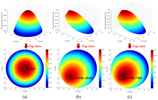
Figure 15.
Irradiance maps for different models. (a) Irradiance map of the Lambertian model; (b) Irradiance map of the Asymmetry model (only radiance non-uniformity); (c) Irradiance map of the Asymmetry model (radiance non-uniformity and stray light non-uniformity).
As illustrated in Figure 15a, in the Lambertian model, it is assumed that all radiances LS are constants. By means of an iterative calculation based on Equation (3), it is possible to obtain a three-dimensional surface diagram and a top view of the irradiance distribution, as illustrated in Figure 15a. The shape of the irradiance distribution in the three-dimensional surface diagram is similar to that of an elliptical mountain peak. The strongest irradiance point is located at the center point (0,0), while the weakest irradiance appears at the edge (x2 + y2 = 202). This characteristic indicates that the irradiance decreases gradually from the center to the edge. In particular, the irradiance change in the central area is relatively gentle, while the irradiance change in the edge area is more significant. This reflects the characteristics of the “center intensification” in the Lambertian model.
Figure 15b illustrates the three-dimensional shape of the irradiance map, which can be described as a mountain peak with varying slopes on either side. The side in closer proximity to the center of the map exhibits a slower rate of decline, whereas the side in closer proximity to the edge of the map exhibits a faster rate of decline. The peak value is located at NA(−10,00,−10.00), which is consistent with the coordinates of the strongest point N in the radiance matrix. This indicates that the non-uniform distribution of radiance affects irradiance beyond the central intensification effect of the Lambertian model. By adjusting the value of RR, it is possible to observe the trend of NA towards the center. From the top view of Figure 15b, it can be observed that the contours of the irradiance distribution undergo a transformation from circular to elliptical. This phenomenon can be attributed to the central intensification effect and the non-uniform distribution of radiance.
Figure 15c illustrates the final irradiance distribution under the Asymmetry model. The three-dimensional map becomes increasingly smooth, and the peak NS shifts towards the center and becomes NS(−7.80,−7.80). The top view reveals that the elliptical contours become flatter, which is a consequence of three factors: central intensification, non-uniform radiance distribution, and stray light. It is noteworthy that, as illustrated in Figure 15a–c, the normalized minimum value of irradiance is observed to decrease. This indicates that the uniformity is also decreasing.
Figure 15 illustrates the pivotal role of the specific position of point N in determining the highest irradiance point of the final Asymmetry model. Furthermore, the coordinates of this position have a significant impact on the overall uniformity of radiance. If point N is situated closer to the edge (x2 + y2 = 202), the proportion of low-radiance areas increases. This results in a reduction in the uniformity of radiance as distance increases. When point N is situated at the center (x1 = 0, y1 = 0), the uniformity of irradiance is at its optimum.
At a distance of 1000 mm (z = 1000 mm), the aperture conversion coefficient K of the illumination light path, calculated according to Equation (6), is 2.52 × 10⁻⁴. In the context of asymmetric simulation conditions, the value of K is observed to range from 2.47 × 10⁻⁴ to 2.47 × 10⁻⁴. The actual range is slightly lower than the theoretical value, primarily due to the influence of stray light and the non-uniformity of the IS radiance being smaller than theoretical expectations. This result is consistent with theoretical predictions and serves to verify the rationality of the Asymmetry model. The optimal values of the final model’s parameters are presented in Table 3.
Table 3.
Optimal parameters of the WHUIS.
4. Experiment
In order to assess the performance of the WHUIS, this study devised a series of bespoke measurement methods and experimental devices with the objective of evaluating the uniformity and dynamic range of the irradiance field at the WHUIS light outlet.
4.1. Experiment Equipment
The assessment of uniformity for the irradiance source can be conducted using point-by-point scanning with a colorimeter or detector, or alternatively, using a calibrated imaging camera. However, imaging cameras lack the capacity to conduct high-uniformity calibration experiments. Consequently, this study opted to employ the detector point-by-point scanning method to obtain comprehensive irradiance maps on the detector disk.
When measuring IS uniformity, it is critical to limit the FOV to ensure accurate calculation of the radiation transfer from the light source to the detector. The National Institute of Metrology of China used dual precision aperture diaphragms to limit the size of the field of view and successfully measured the irradiance uniformity of LED-ISLS [27]. Researchers such as Martin Vacula used a dual aperture tube combined with a detector to evaluate the irradiance uniformity of the extended ultraviolet IS system [28]. This dual aperture diaphragm radiation detection method has been widely used in remote sensing to calibrate ISs.
However, given that the maximum angle of the light outlet of the ILP designed in this study is only 2.86°, a bare detector was chosen for measurement. The WHUIS light source system has the ability to maintain its directionality during propagation outside the light source outlet, which means that the light source system has good collimation in the IS light source. The structural design of the illuminated light path ensures the realization of the design parameters through precise machining and assembly and a series of measurements to ensure good collimation of the light source.
As illustrated in Figure 15, this experiment employs a photoreceptor from the FEMOTO (Novo Hamburgo, Brasil), which has a photosensitive area of 1.1 mm2 and a wavelength range covering 320–1100 nm. For the purpose of positioning, a high-precision linear translation stage from Zolix was employed, which is sufficiently accurate for the intended measurement. The resulting current signal is then obtained using an electrometer (Keithley-6517b, Keithley Instruments, Cleveland, OH, USA) and transmitted through a data collector.
4.2. Experiment Setup
The experimental setup is depicted in Figure 16. It is imperative that all testing be conducted in a dark room, with the optical table and electronic equipment padded with a matte black cloth. The output of the light source system is set to the Z-axis, and the aperture exit plane is the X-Y plane. The detector is aligned with the Z-axis and scanned point by point in a parallel manner to the X-Y plane in order to obtain an irradiance map. In addition, when calibrating the uniformity of the detector’s response, the detector is 5 mm away from the light source outlet.
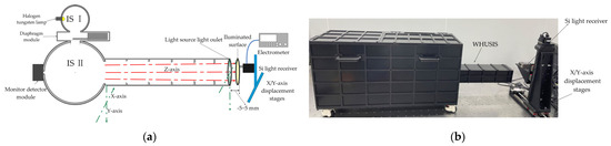
Figure 16.
Schematic diagram of uniformity test of the experimental device. (a) Schematic side view of the experimental device for testing the uniformity of the light source; (b) Actual photo of the test light source (not in test state).
Before measuring uniformity, it is necessary to adjust the detector to be parallel to the optical axis of the equipment, which is defined as the Z-axis. This can be accurately adjusted with the assistance of a laser alignment tool and a level. The stacked scanning method is a commonly employed approach for measuring the irradiance uniformity of the IS output.
The uniformity of the IS is typically quantified using the partition interval method, which divides the measurement area into discrete units, such as an 11 × 11 grid unit (a total of 121 points). Based on previous experience, the experiment set 5 mm intervals and constructed a 13 × 13 grid, forming a 60 × 60 mm square measurement area to cover a measurement area of 50 mm in diameter.
Once the uniformity collection has been completed, the detector should be moved to the center of the light outlet, and dynamic range measurements should be performed. First, adjust the position of the aperture module to the zero position, then gradually open the aperture hole, and record the irradiance corresponding to each motor step.
4.3. Experiment Results and Discussion
Figure 17 illustrates that the irradiance change curve of the light source system exhibits a trend of rapid initial increase, followed by gradual stabilization. This changing trend is a consequence of the mechanism in Equation (2), which adjusts the radiance by modifying the overlap area. Consequently, when undertaking experimental calibration, it is of paramount importance to ensure that a greater number of sampling points are established at the outset of the stroke and that the irradiance is accurately calibrated.
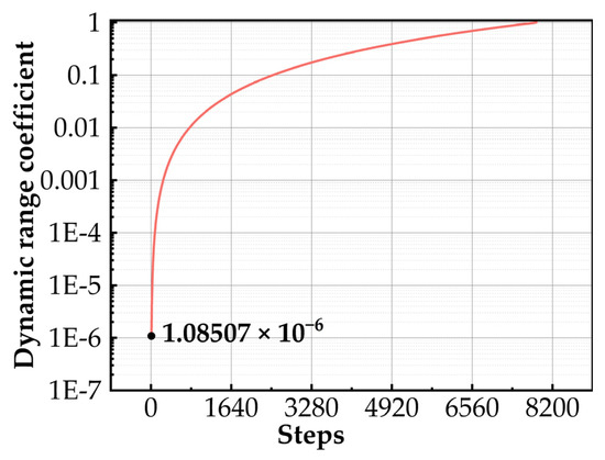
Figure 17.
Experimental results of the irradiance output dynamic range curve.
Furthermore, due to the unavoidable small amount of light leakage and the inevitable machining errors in the design of the diaphragm module, the minimum radiance value in the experiment is approximately two orders of magnitude higher than the simulated value. The level of light leakage has been controlled to the order of 10−6, and the dynamic range factor of irradiance has reached 1.085 × 10⁻⁶, which indicates that the system is capable of achieving a wide dynamic range output of more than six orders of magnitude.
Figure 18a shows the distribution of irradiance at a distance of 5 mm from the light outlet of the source system with a diameter of 40 mm. The collected sample consists of 169 points (13 × 13), of which 81 (9 × 9) are black balls. The data of 81 points (9 × 9 grid) were used to draw a three−dimensional surface map of irradiance, which is smoothed and normalized (the maximum irradiance is set to 1) to present the distribution information of irradiance in the 40 × 40 mm area.
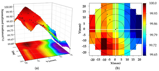
Figure 18.
Irradiance map on the output plane of the WHUIS. (a) Three−dimensional surface plot of irradiance distribution; (b) Two−dimensional plan view of measured irradiance distribution.
As illustrated in Figure 18a, the irradiance distribution within the square area exhibits a peak shape, reaching a maximum value near the (−15, −10) point, and then gradually decreasing towards the edge. For further details on the distribution, please refer to the two-dimensional projection map below the three-dimensional surface.
Figure 18b depicts the irradiance collection grid, comprising 81 sampling points. Of these, 69 are located in a circular area with a diameter of 40 mm, while the remaining points are deemed irrelevant. The black circles numbered 1, 2, 3, and 4 indicate the areas where the light outlet accounts for 80%, 60%, 40%, and 20%, respectively. The axes are demarcated by two white lines, and the origin is situated at the center of the light outlet. Similarly, the irradiance data are normalized such that the maximum value is 100%. It can be observed that the irradiance in the third quadrant is the strongest, while that in the fourth quadrant is the weakest.
Figure 19a,b illustrate the irradiance changes along the X-axis and Y-axis directions at −10, −5, 0, 5, and 10 mm, respectively. The results indicate that the normalized irradiance curve in the X-axis direction exhibits a pattern of an initial increase, subsequent decline, and subsequent stabilization, with the peak value observed at X = 15 mm. In contrast, the curve of the Y-axis undergoes a more pronounced change, with a gentle initial rise followed by a sharp decline.
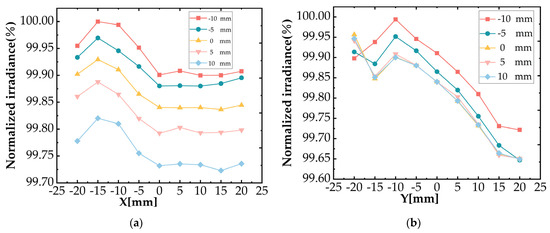
Figure 19.
Irradiance distribution change curves along the axes. (a) Irradiance distribution change curve along the X-axis; (b) Irradiance distribution change curve along the Y-axis.
When considered collectively, the irradiance distribution within a 40 mm circular area is comparable to the distribution characteristics predicted by the model, although there are subtle discrepancies. The disparity can be attributed to three primary factors. The first factor contributing to the discrepancy is the phenomenon of nonlinear changes in the actual radiance distribution. The second reason is that the stray light distribution in the illumination light path is largely related to the BRDF model of the coating. However, the model does not take this factor into account. The third reason is due to practical considerations, such as processing errors, the reflectivity of the inner surface of the light source, and avoidable measurement errors.
Table 4 presents a summary of the irradiance uniformity U within different areas. Within 80% of the area with a diameter of 40 mm, the uniformity reaches 99.9029%, which is in line with the expectations of the Asymmetry model and meets the 99.8% irradiance uniformity standard required by the CHES. It further proves that the collimation of the WHUIS light source system can satisfy the needs of use.
Table 4.
Evaluation values of uniformity for different regions.
With regard to the uniform value of the asymmetric model in a smaller area, there is a slight overestimation. This discrepancy can be attributed to three factors. First, the number of samples in a small area is relatively limited. Second, the results are influenced by unavoidable factors such as detector stability and light source stability. Third, the model is designed for the estimation of uniformity within a diameter of 40 mm, with smaller weights being given to uniformity estimates considering small areas.
In conclusion, the WHUIS achieves high uniformity of irradiance within a 40 mm diameter circular area, with a dynamic range of six orders of magnitude. The experimental results of the irradiance distribution are generally consistent with the model predictions, which further proves the effectiveness of the Asymmetry model in simulating long-distance irradiance transfer in the closed light source based on IS.
5. Conclusions
This paper presents research on the design, analysis, and testing of a wide dynamic range, high uniformity spectral irradiance source (WHUIS), which is based on the requirements for precise calibration of the non-uniformity of scientific-grade, large-size matrix detectors. The paper then goes on to present the structural components of the WHUIS, including the cascade integrating sphere, diaphragm module, and illumination light path. An irradiance transfer simulation model is proposed based on the working principle and structural composition of the WHUIS. The contributions of relative distance, radiance distribution, stray light, and other factors to the non-uniformity of irradiance output are analyzed. Furthermore, design parameter optimization was performed using the model. A test device was constructed with the objective of measuring the uniformity of irradiance output from the WHUIS and verifying the rationality of the Asymmetry model and the performance of instrument. The simulation analysis yielded results that were consistent with the test results. The irradiance output uniformity of the WHUIS is greater than 99.9% within a 40 mm circular area, with a dynamically adjustable range of six levels of constant color temperature.
Future work will involve utilizing the exceptional uniformity of WHUIS irradiance output to investigate the precise calibration technology required for the radiation response characteristics of scientific-grade, large-scale space detectors.
Author Contributions
Conceptualization, D.K. and Y.Y.; design, D.K. and Y.Y.; writing—original draft preparation, D.K.; modeling, simulation and experiment, D.K.; writing—review and editing, D.K. and X.Z.; funding acquisition, Y.Y. and H.L.; guidance on instrument machining, W.Z. All authors have read and agreed to the published version of the manuscript.
Funding
This research was funded by the National Natural Science Foundation of China (42375123) and the Chinese Academy of Sciences Strategic Pilot Project for Space Science (XDA15020800).
Data Availability Statement
The original contributions presented in the study are included in the article, further inquiries can be directed to the corresponding author.
Acknowledgments
We are very grateful to Zhen Liu for his comments on the scientific presentation of the article and the standardization of the formulas.
Conflicts of Interest
The authors declare no conflicts of interest.
References
- Ji, J.; Wang, S.; Li, H.; Fang, L.; Li, D. CHES: An astrometry mission searching for nearby habitable planets. Innovation 2022, 3, 1–2. [Google Scholar] [CrossRef] [PubMed]
- Ji, J.-H.; Li, H.-T.; Zhang, J.-B.; Fang, L.; Li, D.; Wang, S.; Cao, Y.; Deng, L.; Li, B.-Q.; Xian, H. CHES: A space-borne astrometric mission for the detection of habitable planets of the nearby solar-type stars. Res. Astron. Astrophys. 2022, 22, 072003. [Google Scholar] [CrossRef]
- Jiang, Y.; Tian, J.; Fang, W.; Hu, D.; Ye, X. Freeform reflector light source used for space traceable spectral radiance calibration on the solar reflected band. Opt. Express 2023, 31, 8049–8067. [Google Scholar] [CrossRef] [PubMed]
- Voigt, D.; Hagendoorn, I.; van der Ham, E. Compact large-area uniform colour-selectable calibration light source. Metrologia 2009, 46, S243. [Google Scholar] [CrossRef]
- Zheng, R.; Li, C.; Gao, Y.; Li, G.; Liu, B.; Sun, K. Design of Optical System of Infrared Star Simulator Uniform Radiation Under Specific Irradiance. Acta Photonica Sin. 2022, 51, 24–32. [Google Scholar] [CrossRef]
- Yamaguchi, Y.; Yamada, Y.; Ishii, J. Supercontinuum-source-based facility for absolute calibration of radiation thermometers. Int. J. Thermophys. 2015, 36, 1825–1833. [Google Scholar] [CrossRef]
- Anhalt, K.; Zelenjuk, A.; Taubert, D.; Keawprasert, T.; Hartmann, J. New PTB setup for the absolute calibration of the spectral responsivity of radiation thermometers. Int. J. Thermophys. 2009, 30, 192–202. [Google Scholar] [CrossRef]
- Yoon, H.; Gibson, C.; Eppeldauer, G.; Smith, A.; Brown, S.; Lykke, K. Thermodynamic radiation thermometry using radiometers calibrated for radiance responsivity. Int. J. Thermophys. 2011, 32, 2217–2229. [Google Scholar] [CrossRef]
- Mikheenko, L.; Borovytsky, V. Metrological advantages of the light source based on optically connected integrating spheres. In Infrared Remote Sensing and Instrumentation XX; SPIE Optical Engineering + Applications: San Diego, CA, USA, 2012; pp. 265–276. [Google Scholar] [CrossRef]
- Wang, S.; Shi, J.; Li, H.; Zhang, B.; Xie, Q.; Sun, Y. Weak light uniform light system for LLL ICCD parameter calibrating device. J. Appl. Opt. 2016, 37, 818–822. [Google Scholar] [CrossRef]
- Yongqiang, L.; Zhanping, Z.; Pengmei, X.; Jingyi, W.; Yongxiang, G. Radiometric calibration of large dynamic range low light level camera. Infrared and Laser Engineering, Papers 2019, 48.
- Durell, C.; Scharpf, D. Integrating Sphere Theory; Labsphere: North Sutton, NH, USA, 2020. [Google Scholar]
- Cooper, J.W.; Brown, S.W.; Abel, P.; Marketon, J.E.; Butler, J.J. Radiometric characterization of the NASA GSFC Radiometric Calibration Facility primary transfer radiometer. In Sensors, Systems, and Next-Generation Satellites VIII; SPIE Optical Engineering + Applications: San Diego, CA, USA, 2004; pp. 472–481. [Google Scholar]
- Chen, J.; Sun, G.; Liu, S.; Zhang, G.; Chen, S.; Zhang, J.; Liu, Q. Design of Integrating Sphere Uniform Light System for Solar Simulator. IEEE Photonics J. 2023, 15, 1–7. [Google Scholar] [CrossRef]
- Labsphere, A. Guide to Integrating Sphere. In Theory and Applications; Labsphere: North Sutton, NH, USA, 2012. [Google Scholar]
- Tang, C.; Meyer, M.; Darby, B.L.; Auguié, B.; Le Ru, E.C. Realistic ports in integrating spheres: Reflectance, transmittance, and angular redirection. Appl. Opt. 2018, 57, 1581–1588. [Google Scholar] [CrossRef] [PubMed]
- Zha, G.; Wu, H.; Li, J.; Yuan, Y. Angular uniformity of cascaded integrating sphere radiation source. J. Appl. Opt. 2022, 43, 481–487. [Google Scholar]
- Fest, E. Stray Light Analysis and Control; SPIE Optical Engineering + Applications: San Diego, CA, USA, 2013. [Google Scholar]
- Freniere, E.R. First-order design of optical baffles. In Radiation Scattering in Optical Systems; SPIE Optical Engineering + Applications: San Diego, CA, USA, 1981; pp. 19–28. [Google Scholar]
- Breault, R.P. Vane structure design trade-off and performance analysis. In Stray Light and Contamination in Optical Systems; SPIE Optical Engineering + Applications: San Diego, CA, USA, 1989; pp. 90–117. [Google Scholar]
- Vacula, M.; Horvath, P.; Chytka, L.; Daumiller, K.; Engel, R.; Hrabovsky, M.; Mandat, D.; Mathes, H.-J.; Michal, S.; Palatka, M. Optical ray-tracing simulation method for the investigation of radiance non-uniformity of an integrating sphere. Optik 2023, 291, 171350. [Google Scholar] [CrossRef]
- Zalewski, E.F. Radiometry and photometry. Handb. Opt. 1995, 2, 24.21–24.51. [Google Scholar]
- Jacobs, V.; Blattner, P.; Ohno, Y.; Bergen, T.; Krüger, U.; Hanselaer, P.; Rombauts, P.; Schmidt, F. Analyses of errors associated with photometric distance in goniophotometry. In Proceedings of the 28 Session of CIE, Manchester, UK, 28 June–4 July 2015; pp. 458–468. [Google Scholar]
- Jähne, B. Release 4 of the EMVA 1288 standard: Adaption and extension to modern image sensors. In Forum Bildverarbeitung 2020; Heizmann, M., Längle, T., Eds.; KIT Scientific Publishing: Karlsruhe, Germany, 2020; pp. 13–24. [Google Scholar]
- Li, Y.; Liu, Z.; Yuan, Y.; Zhai, W.; Zou, P.; Zheng, X. Nonlinearity Measurement of Si Transferring Photodetector in the Low Radiation Flux Range. Photonics 2023, 10, 1015. [Google Scholar] [CrossRef]
- Luo, S.; Zeng, Y.; Chen, J.; Luo, L.; Tang, S. Simulation and experimental research on the uniformity of the surface light source out from the integrating sphere. In Proceedings of the 9th International Symposium on Advanced Optical Manufacturing and Testing Technologies: Meta-Surface-Wave and Planar Optics, Chengdu, China, 26–29 June 2018; pp. 136–141. [Google Scholar]
- Fu, Y.; Liu, X.; Wang, Y.; He, Y.; Feng, G.; Wu, H.; Zheng, C.; Li, P.; Gan, H. Miniaturized integrating sphere light sources based on LEDs for radiance responsivity calibration of optical imaging microscopes. Opt. Express 2020, 28, 32199–32213. [Google Scholar] [CrossRef]
- Vacula, M.; Horvath, P.; Chytka, L.; Daumiller, K.; Engel, R.; Hrabovsky, M.; Mandat, D.; Mathes, H.-J.; Michal, S.; Palatka, M. Use of a general purpose integrating sphere as a low intensity near-UV extended uniform light source. Optik 2021, 242, 167169. [Google Scholar] [CrossRef]


Disclaimer/Publisher’s Note: The statements, opinions and data contained in all publications are solely those of the individual author(s) and contributor(s) and not of MDPI and/or the editor(s). MDPI and/or the editor(s) disclaim responsibility for any injury to people or property resulting from any ideas, methods, instructions or products referred to in the content. |
© 2024 by the authors. Licensee MDPI, Basel, Switzerland. This article is an open access article distributed under the terms and conditions of the Creative Commons Attribution (CC BY) license (https://creativecommons.org/licenses/by/4.0/).