Article

EWMACD Algorithm in Early Detection of Defoliation Caused by Dendrolimus tabulaeformis Tsai et Liu

1
School of Information Engineering, China University of Geosciences, Beijing 100083, China
2
Chongqing Institute of Green and Intelligent Technology, Chinese Academy of Sciences, Chongqing 400714, China
3
Chongqing Rural Commercial Bank Co., Ltd., Chongqing 400023, China
*
Author to whom correspondence should be addressed.
Remote Sens. 2024, 16(13), 2299; https://doi.org/10.3390/rs16132299
Submission received: 20 May 2024 / Revised: 14 June 2024 / Accepted: 20 June 2024 / Published: 24 June 2024
(This article belongs to the Section Forest Remote Sensing)

Abstract

:
The persistent increase in forest pest outbreaks requires timely detection methods to monitor the disaster precisely. However, early detection is challenging due to insufficient temporal observation and subtle tree changes. This article proposed a novel framework that collaborates multi-source remote sensing data and uses a change detection algorithm to archive early detection of infestation caused by Dendrolimus tabulaeformis Tsai et Liu (D. tabulaeformis) attacks. First, all available Sentinel-2 images with less than 20% cloud cover were utilized. During periods with long intervals (>16 days) between Sentinel-2 images, Landsat-8 images with less than 20% cloud cover were downscaled to a spatial resolution of 10 m using a deep learning algorithm to meet the requirement for a high temporal frequency of clear observations. Second, the spectral index differences between healthy and infested trees were examined to address the challenge of detecting subtle changes in pest attacks. The Enhanced Vegetation Index (EVI) was selected for early defoliation detection. On this basis, the EWMACD (Exponentially Weighted Moving Average Change Detection) algorithm, which is sensitive to subtle changes, was enhanced to improve the capability of detecting early D. tabulaeformis attacks. The assessment showed that the overall accuracy of the change detection (F1 score) reached 0.86 during the early stage and 0.88 during the late stage. The temporal accuracy (Precision) was 84.1% during the early stage. The accuracy significantly improved compared to using a single remote sensing data source. This study presents a new framework capable of monitoring early forest defoliation caused by D. tabulaeformis attacks and offering opportunities for predicting future outbreaks and implementing preventive measures.

1. Introduction

Chinese pine (Pinus tabulaeformis) is one of the endemic coniferous species in China. With increasing stand age and environmental changes, forest pests and pathogens, especially Chinese pine Caterpillar (Dendrolimus tabulaeformis Tsai et Liu, D. tabulaeformis) have become increasingly severe and have killed a significant number of pine trees [1]. This has resulted in substantial losses and persistent threats to forestry, impacting services, structure, carbon, and functionality of forest ecosystems [2,3,4]. D. tabulaeformis is a defoliating pest with a rapid rate of spread [5]. Widespread defoliation could potentially occur in just one month [6]. Therefore, early warning for D. tabulaeformis is crucial for timely intervention. Because of the widespread coverage of pine forests and the high spread area of this pest infestation, traditional forestry inventory methods, such as trapping of larvae, are difficult to conduct and the spatiotemporal observation scale of the results is insufficient [7].
Previously, monitoring forest pests typically used hyperspectral data or high-spatial-resolution multispectral data [2,8]. However, the limited time frequency and high cost make it usually not suitable for large-scale analysis. The changes in crowns caused by pest infestation are gradual and subtle. It could be best characterized through time series analysis [9]. Some scholars have applied time series data with coarse spatial resolution but high temporal resolution, such as MODIS [10,11,12]. This method sacrifices spatial resolution, making it difficult to delineate the area of infestation. Due to its free availability and long-term monitoring capabilities, Landsat data is frequently used for forest pest monitoring [13,14,15]. However, the influence of cloud cover can sometimes result in the actual revisit period of Landsat data exceeding 16 days. Missing one image could lead to missing the entire early stage of pest infestation (≈30 days). With the launch and free data access of the Sentinel-2A and -2B sensors, Sentinel-2 data is widely used for pest monitoring [16,17,18]. However, the insufficient data spatiotemporal resolution used in current research limits the spatiotemporal accuracy of pest monitoring. The location provided by studies based on coarse spatial resolution images is not accurate enough. The studies based on finer spatial resolution images have the potential to improve identification accuracy, such as the results from Daniele et al. [18], and the monitoring results are close to monthly temporal resolution. There is still room for improvement in the monitoring frequency, which is crucial for early pest infestation detection.
To address the insufficient spatiotemporal resolution of observations from a single data source, some scholars have advanced their research by integrating multi-source remote sensing data to obtain denser time series data. Shang et al. [19] near-real-time monitored forest disturbance with harmonized Landsat-7, -8 and Sentinel-2 data. Christopher et al. [20] utilized a Harmonized Landsat Sentinel-2 (HLS) dataset with a temporal resolution of 7 days to monitor forest changes in high-latitude regions. However, previous studies mostly resampled the finer-resolution image to match the coarser-resolution image when integrating data with different spatial resolutions. This approach sacrifices the image’s spatial resolution in exchange for higher temporal resolution [21]. Currently, deep learning-based super-resolution reconstruction is one of the most popular image fusion methods, enabling images to be collaborative at high spatial resolution. Zhang et al. [22] utilized deep learning to fuse Sentinel-2 and Landsat images to track small-scale tropical forest disturbances and mapped the disturbance with a spatial resolution of 10 m. It detected 11% to 21% more disturbance areas compared to using Sentinel-2 or Landsat-7/8 time series alone. Therefore, using deep learning algorithms to downscale low-resolution data and collaborate with high-spatial-resolution data can increase observation frequencies, thereby timely monitoring early pest infestations.
Because the subtle and gradual changes are difficult to detect, current research has developed change detection algorithms sensitive to pest infestations to detect early forest pest outbreaks. Huo et al. [23] proposed a novel vegetation index to detect early European spruce bark beetle infestations based on Sentinel-1 and -2 images. The method achieved identification accuracy ranging from 0.80 to 0.82 during the early stages of infestation. Vojtěch et al. (2021) [24] utilized the random forest algorithm to conduct classification between healthy and bark-beetle-infected trees based on Sentinel-2 images, achieving a 78% overall accuracy in the classification. Christopher et al. [20] employed the BEAST algorithm to monitor forest changes in high-latitude regions. The results indicate that this method can serve as an early warning signal for changes caused by pest infestation. However, most of the aforementioned methods still need improvement in terms of sensitivity to early pest infestations. In studies such as [13], over 50% of Landsat pixels are detected during the transition period between green (early stage) and red/gray stages after being infested, which greatly affects the response speed and accuracy. In studies such as [24,25,26], the accuracies of green-attack (early) stages detection are significantly lower than red or grey-attack stages, which could reach 90% [27,28]. These studies point to a large insufficient in early infestation detection. Identifying such subtle changes often requires more sensitive approaches. The EWMACD (Exponentially Weighted Moving Average Change Detection) algorithm is a change detection algorithm sensitive to subtle changes based on time series data. It has been used to identify minor disturbances in forests, such as selective logging [29,30]. Research has also confirmed the potential of using the EWMACD algorithm for detecting pest infestations [31]. Therefore, the EWMACD algorithm has the feasibility to monitor early D. tabulaeformis infestation.
The objective of this study is to achieve early warning of D. tabulaeformis infestations through collaborative multi-source remote sensing time series data and apply EWMA (Exponentially Weighted Moving Average) change detection algorithm. By collaborating Sentinel-2 and Landsat-8 data, higher temporal resolution time series could be obtained, enabling timely and spatially explicit monitoring of D. tabulaeformis infestation. On this basis, sensitive features of infestation are extracted, and the EWMA change detection algorithm, which is sensitive to subtle changes, is applied to achieve early warning and accurate detection.

2. Materials and Methods

2.1. Study Area

The study area, the mid-west part of Lingyuan City, is located in Liaoning Province, China (Figure 1). Lingyuan City has a total forest area of 136,000 hectares, of which 69,600 hectares are pine forests. The forest in the study area is mostly composed of Pinus tabulaeformis, covering a total area of 3335 hectares. The average temperature in March 2018 was 6.39 °C, and the average temperature in October 2018 was 16.58 °C. As a primary tree species for afforestation on barren hills, Pinus tabulaeformis forests are predominantly artificial pure forests [32,33]. D. tabulaeformis infestation broke out in 2018, with one generation occurring each year in the study area. D. tabulaeformis began climbing trees from mid-March to mid-April after overwintering, feeding on pine needles in small quantities, marking the early stage of infestation. In mid-June, they begin pupation, with adults emerging in early July to lay eggs, during which time they do not harm pine trees. Larvae start appearing from late July to mid-August, feeding extensively on pine needles, displaying the most severe damage, indicating the late stage of infestation. By early October, D. tabulaeformis started descending from trees to overwinter.

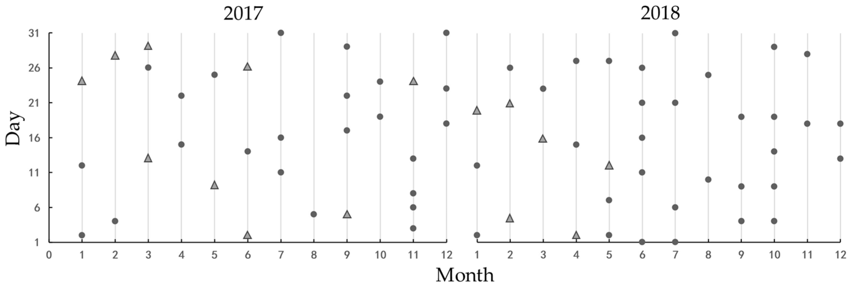
2.2. Data and Pinus Tabulaeformis Forest Mask

Based on the physiological habits of D. tabulaeformis, the study period is determined to be from 1 March 2018 to 31 October 2018. As described in Section 3.2.2, the change detection algorithm uses information from the target year and the reference year to detect forest pests. Therefore, all Sentinel-2A and -2B images with cloud cover less than 20% in the study area from 2017 to 2018 were collected, totaling 56 images. Additionally, during periods with long intervals (>16 days) between Sentinel-2 images, Landsat-8 images with cloud cover less than 20% in the study area were downscaled, totaling 16 images. The average revisit period during the study period was approximately 8.6 days. Figure 2 shows the temporal distribution of all the images used from 2017 to 2018.
Sentinel-2 Top of Atmosphere (TOA) images were obtained from the European Space Agency (ESA) and then atmospherically corrected using Sentinel Application Platform (SNAP), and converted into surface reflectance (SR) images. Landsat-8 SR images were downloaded from the Google Earth Engine (GEE) platform.
Since the focus of this study is on identifying forest pests, and the forest area in the study area is mostly pure pine forest, the Pinus tabulaeformis forest mask was created based on the Environmental Systems Research Institute (ESRI) land use/land cover (LULC) dataset during 2017 and 2018, along with field-collected Pinus tabulaeformis samples, and used the random forest classification algorithm.

2.3. Training and Validation Data

The training data used for feature selection: a field survey was conducted in October 2018. D. tabulaeformis infestations were identified through visual inspection of pine needle color and signs of feeding. A total of 5 infestation points and 5 healthy points were collected through field measurements, and their locations were recorded. The damage level of the infestation points is severe. Visual interpretation was also conducted based on available Very High Resolution (VHR) images from Google Earth Pro (GEP) and Sentinel-2 images obtained from 2017 to 2018. Combining field surveys and visual interpretation, a total of 200 training data points were selected, with 100 infestation points and 100 healthy points.
The validation data used for accuracy assessment: validation data were selected through visual interpretation based on available VHR images from GEP and Sentinel-2 images from 2017 to 2018. A total of 100 validation points were selected for both the early and late stages of infestation, with 50 infestation points and 50 healthy points for each stage.

3. Methodology

The overall workflow of this study is illustrated in Figure 3. Firstly, Sentinel-2 images were preprocessed to obtain surface reflectance data. Then, based on the ESRCNN data fusion algorithm, Landsat-8 images were fused with Sentinel-2 images to generate a dense time series with a spatial resolution of 10 m (see Section 3.1). Next, for each pixel, the Enhanced Vegetation Index (EVI), Normalized Burn Ratio (NBR), Red-Green Index (RGI), and SWIR2 were calculated. Then the Jeffries–Matusita (JM) distance for the indices in both healthy and infested points were computed (see Section 3.2.1). EVI was selected as the optimal input feature and EVI time series data were input into the Exponentially Weighted Moving Average Change Detection (EWMACD) algorithm. Infestation is detected when the EWMA value consistently exceeds the control limit (see Section 3.2.2). Finally, post-processing is applied to the detection results, followed by an accuracy assessment (see Section 3.3). The following sections will delve into the key processes in detail.

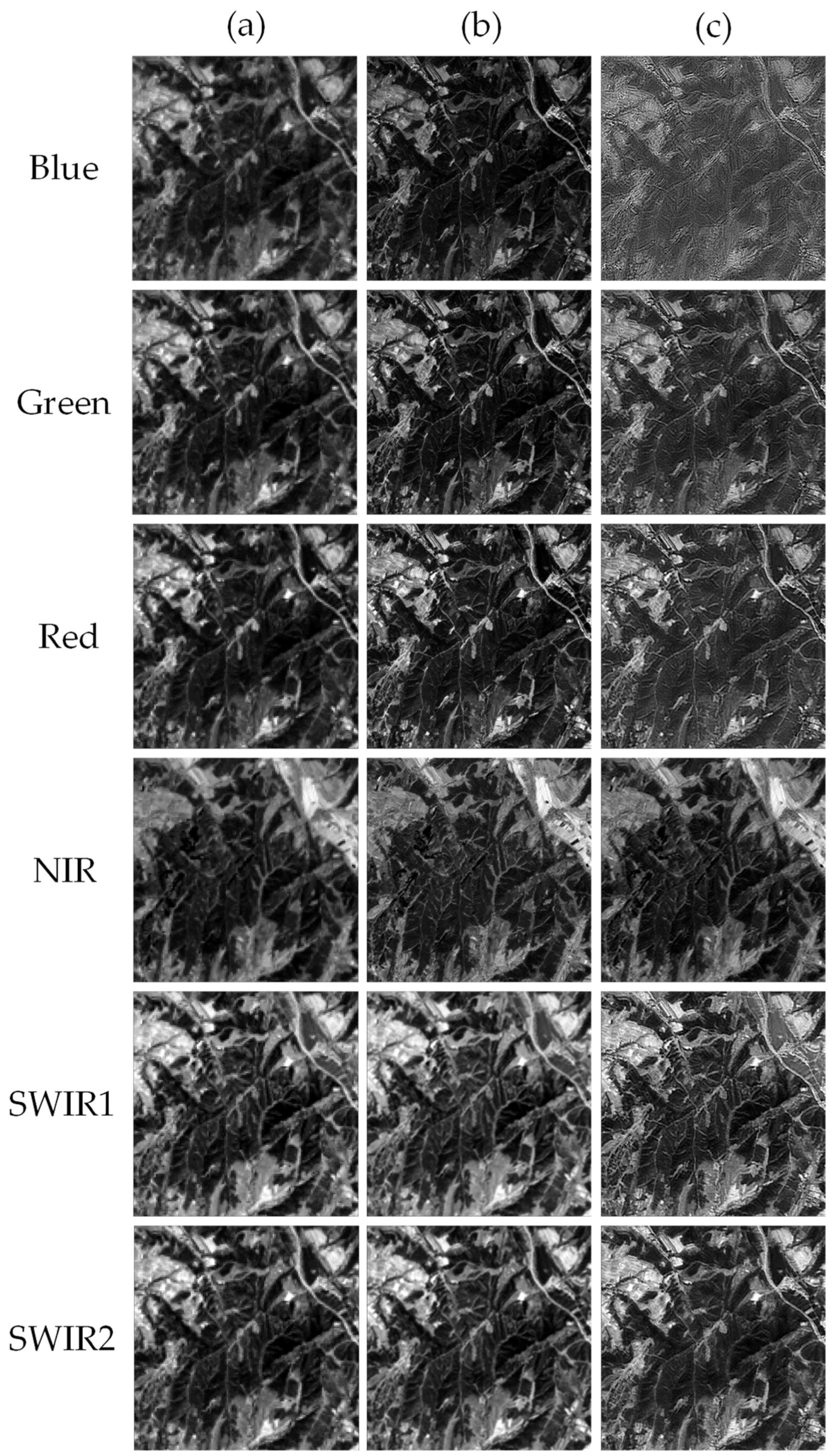
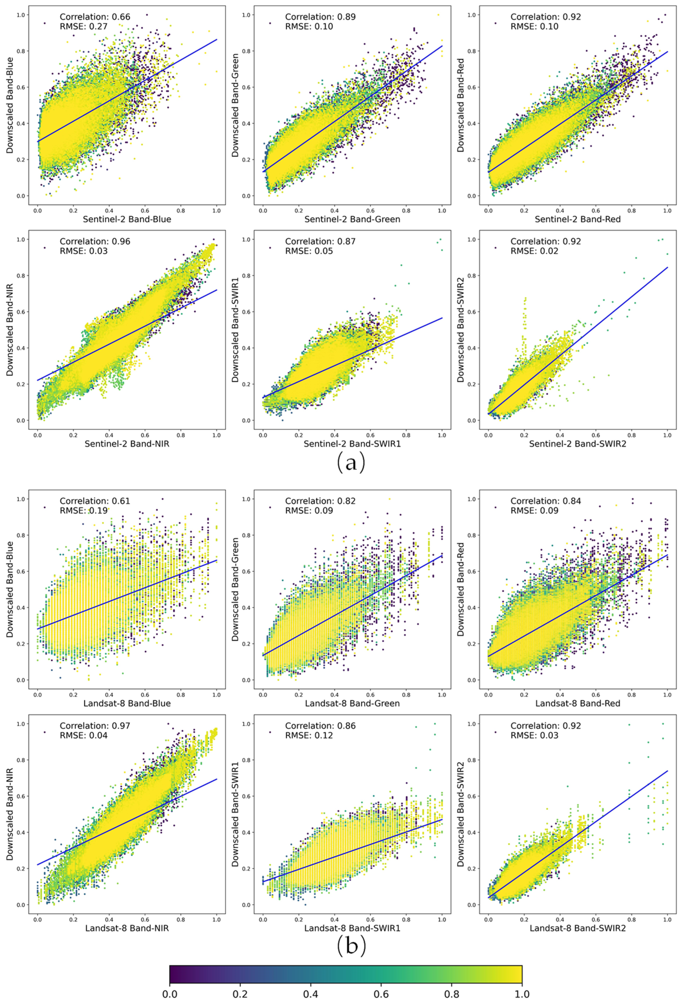
3.1. Fusion of Sentinel-2 and Landsat-8

Collaborating multi-source data could enhance the temporal resolution of observations, enabling timely observation. To harmonize the resolution disparities between images from different sources, data fusion algorithms could downscale coarse spatial resolution images to match fine spatial resolution images. Therefore, the ESRCNN algorithm proposed by Shao et al. [34] based on deep learning for image super-resolution reconstruction can automatically select the optimal features from one or multiple images for high spatial resolution reflectance prediction. Compared to previous algorithms such as STARFM and ATPRK [35,36], ESRCNN improves image quality and preserves the reflectance distribution of the original images better.
ESRCNN uses fine-resolution Sentinel-2 image as auxiliary data to downscale the coarse-resolution Landsat-8 image. Firstly, ESRCNN employs an adaptive fusion algorithm, instead of the simple resampling method, to downscale Sentinel-2 image bands 11–12 from 20 m to 10 m resolution. Secondly, ESRCNN utilizes Landsat-8 panchromatic bands and Sentinel-2 bands 2–4, 8, and 11–12 to downscale Landsat-8 bands 1–7. This fusion network is designed to accommodate flexible numbers of Sentinel-2 images as auxiliary datasets. In this article, for each downscaling of the Landsat-8 image, three auxiliary Sentinel-2 images are required. Table 1 displays the dates of downscaled Landsat-8 images and auxiliary Sentinel-2 images.
The data fusion results were evaluated by comparing the spatial distribution and spectral value between the fused images and the reference images (Sentinel-2 image on the same or near date). Root Mean Square Error (RMSE) and the Pearson correlation coefficient (Correlation) were used to assess the accuracy of reflectance values. These two metrics are widely employed for evaluating the performance of data fusion algorithms.
The RMSE is used to evaluate the spectral difference between the reference image and the fused image. RMSE is calculated as:
R M S E ( R , F ) = 1 M N i = 1 M j = 1 N R i , j F ( i , j ) 2
where R represents the reference image, F represents the fused image, M is the number of pixels on the row, and N is the number of pixels on the column.
Correlation is used to indicate the correlation between the reference image and the fused image, calculated as:
C o r r e l a t i o n R , F = i = 1 M j = 1 N R i , j μ ( R ) F i , j μ ( F ) i = 1 M j = 1 N R i , j μ ( R ) 2 i = 1 M j = 1 N F i , j μ ( F ) 2
where μ refers to the mean value.
To validate the applicability of the ESRCNN algorithm for this study, it was necessary to have Sentinel-2 images available on dates close to those of the fusion data. Therefore, we selected Sentinel-2 images collected on 11 July, 16 July, and 31 July 2017 as auxiliary data to downscale the Landsat-8 image collected on 12 July 2017. The result is shown in Figure 4. Visually, the downscaled images exhibit finer spatial details across all bands compared to the original Landsat-8 images. Moreover, the bands closely resemble those of the neighboring Sentinel-2 images.
Figure 5 displays the accuracy assessment results of the downscaled image. Comparing the downscaled images with the original Landsat-8 images and the adjacent date Sentinel-2 images, the RMSE is generally less than 0.1, and the Correlation is generally greater than 0.85. These metrics indicate that the downscaled images are consistent with the original images in terms of spectral and spatial characteristics.

3.2. Defoliation Detection Algorithm

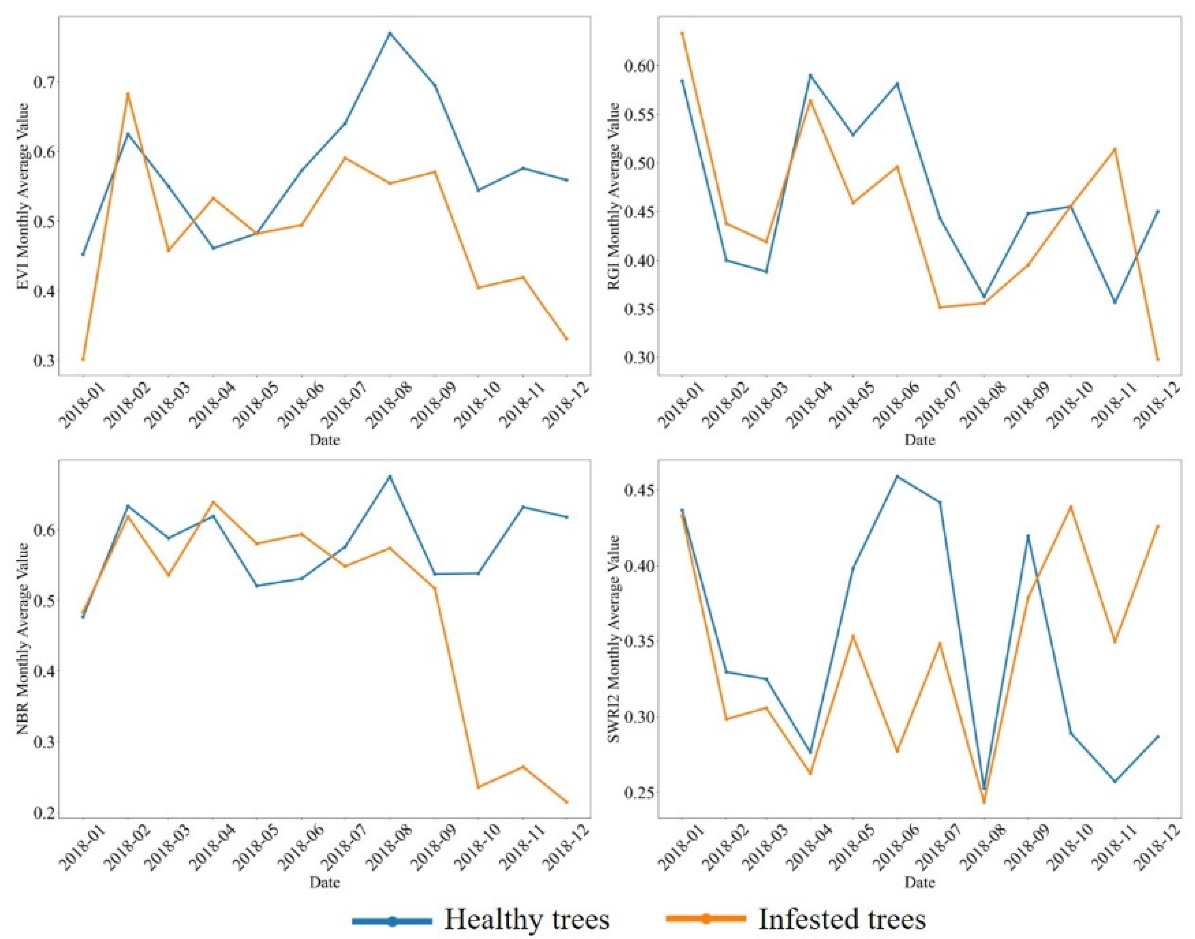
3.2.1. Feature Selection

Selecting features sensitive to D. tabulaeformis infestation is crucial for inputting into the change detection algorithm. D. tabulaeformis infestation results in pine defoliation, needle desiccation, and reduced chlorophyll content. Therefore, we referred to existing studies and selected several vegetation indices and bands (Table 2) related to water stress, color, and needle structure. Using the training dataset, we calculated the Jeffreys–Matusita (JM) distance for each candidate feature in both the early and late stages of the damage.
The JM distance quantifies the separability of selected features between infested and healthy pine forests. It ranges from [0, 2], with higher values indicating greater separability. The JM distance is calculated as:
J M = 2 ( 1 e B )
B = 1 8 ( m i m j ) 2 2 σ i 2 + σ j 2 + 1 2 ln σ i 2 + σ j 2 2 σ i σ j
where B represents the Bhattacharyya Distance, m i , m j represent the mean values, while σ i , σ j respectively represent the standard deviation of a specific feature within the two categories.

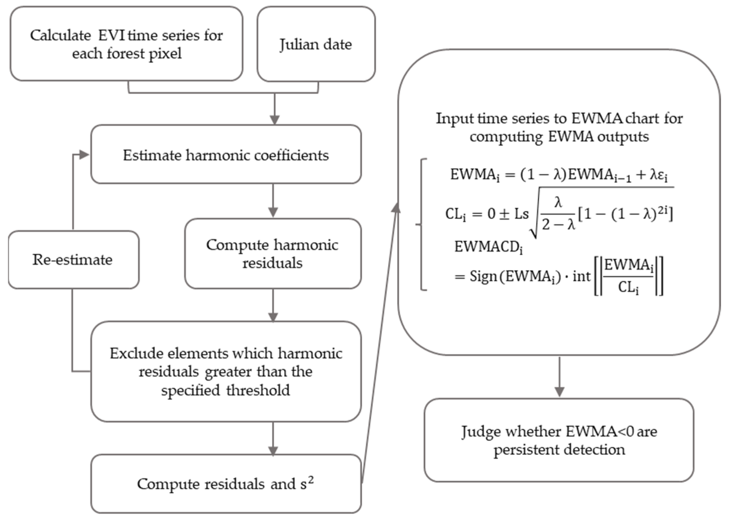
3.2.2. EWMACD Algorithm

EWMACD is an online time series change detection algorithm sensitive to subtle change. The flowchart of EWMACD is illustrated in Figure 6.
Specifically, the EWMACD algorithm first establishes the following harmonic model during training to eliminate the impact of phenological changes on pest monitoring:
y i = a 0 + j = 1 k b j cos 2 π j D t i + c j sin 2 π j D t i + ε i
where y i is EVI value, a 0 is the intercept coefficient, k is the order of harmonic function and set = 2, b j is the coefficient of cosine harmonic, c j is the coefficient of sine harmonic, t i is Julian date, and i = [1, 2, …, N], D is the number of days within a year. ε i represents the regression residual of Julian date. These coefficients are estimated utilizing the ordinary least squares (OLS) method.
Secondly, all elements with standardized residual values greater than the specified threshold were filtered out through the X-Bar value to remove interference from clouds and outliers and then recalculate the harmonic coefficients:
β ^ = ( X t r a i n X t r a i n ) 1 X t r a i n t n t r a i n
where X t r a i n is a matrix composed of n t r a i n × 1 + c i + b j , each harmonic coefficient is adjusted according to the Julian date. After all elements which standardized residuals greater than the threshold are filtered out, β ^ is recalculated. Then, the residuals ( r e s ) were calculated as:
r e s = t X β ^
where X is the matrix derived from computing the full n × ( 1 + c j + b j ) . The training period variance s 2 was calculated as:
s 2 = r e s n t r a i n r e s n t r a i n n t r a i n 1
where r e s n t r a i n represent the residual on the training period.
EWMA values were calculated as:
E W M A i = 1 λ E W M A i 1 + λ ε i
where the E W M A 1 = 0. The smoothing parameter λ ranges from 0 to 1. λ close to 0 indicates that a greater weight of the historical period data, E W M A i , mainly relies on E W M A i 1 . The λ is set to 0.15 (Figure 7).
The control limit of EWMA chart were computed as:
C L i = 0 ± L s λ 2 λ 1 ( 1 λ ) 2 i
where L represents the constant control limit, s represents the standard deviation of all residuals during the training period.
Then, the E W M A C D i was calculated as:
E W M A C D i = S i g n ( E W M A i ) · i n t E W M A i C L i
where S i g n ( ) is used to obtain the plus-minus sign of E W M A i , represents the absolute value, and i n t [ ] represents the integer value. The pest infestation was signaled when EWMACD value less than 0.
It is significant to define smoothing coefficients λ when using the EWMACD algorithm. λ represents the weight of historical period data and affects the calculation of control limits of the EWMA chart, which is directly related to the sensitivity of change detection. Observing the detection result using differences λ in Figure 7, pest infestation was difficult to detect when setting λ high, such as λ = 0.2 (Figure 7d). When λ was set low (e.g., λ = 0.1), a significant increase in misclassified pixels (Figure 7f). Therefore, we will initially set λ to 0.15 as the smoothing coefficient (Figure 7e).

3.3. Accuracy Assessment

To assess the spatial accuracy of early and late detection results of insect damage, the precision (Precision), recall (Recall), overall accuracy (OA), and F1-score were computed as accuracy evaluation metrics based on the validation dataset.
P r e c i s i o n = T P T P + F P
R e c a l l = T P T P + F N
O A = T P + T N T P + F P + T N + F N
F 1 s c o r e = 2 T P 2 T P + F P + F N
where T P represents true positive, F P represents false positive, T N represents true negative, and F N represents false negative.

4. Results

4.1. Feature Selection Results

The time series of each candidate feature, including EVI, NBR, RGI, and SWIR2 were calculated, as shown in Figure 8. The JM distance for the early and late stages of infestation was computed, as shown in Table 3. Throughout the entire study period, EVI was the earliest and most consistent to display spectral differences between healthy and diseased trees. Also, EVI continuously maintained a higher JM distance. As the aim of this study is to achieve early detection of insect damage, considering the comprehensive comparison of time series indices and JM distances, EVI was ultimately chosen as the input feature for detecting pest infestation.

4.2. Feasibility Analysis of Using EWMACD Algorithm for Pest Detection

Figure 9 shows the time series of EVI and EWMA values for a typical infestation pixel to evaluate the feasibility of the EWMACD algorithm for pest detection. In mid-March, the D. tabulaeformis began to return to the pine trees and slightly nibble on the needles, indicating the early-stage onset of pest infestation. The EWMACD algorithm detected the pest occurrence starting from 23 March 2018. In mid-June, the D. tabulaeformis started cocooning and laying eggs after pupating, during which they did not harm the pine trees. The EWMA value remained unchanged from 16 June to 31 July. In late July, the larvae began to voraciously eat the needles, leading to a significant decrease in the EWMA value starting from 10 August. In early October, the D. tabulaeformis began to descend from the trees to hibernate, and the EWMA value gradually recovered from 14 October onwards, stabilizing after 24 October. In summary, the EWMACD algorithm effectively detects pine caterpillar infestation.

4.3. Assessment of Infestation Detection Accuracy

4.3.1. Overall Detection Results of EWMACD

The output of the EWMACD algorithm is a multi-band raster, with each band representing the detection results for the corresponding date. Based on the spatial clustering and temporal persistence of the pest infestation, we applied post-processing to the detection results. We aggregated all raster values for the early detection period (1 March 2018, to 15 April 2018) to obtain the early detection results, and aggregated all raster values for the entire study period (1 March 2018, to 31 October 2018) to obtain the late detection results, while also applying spatial filtering. The early and late detection results of the EWMACD algorithm for the entire study area are shown in Figure 10. The early damaged area is approximately 868 hectares, while the late damaged area is approximately 1183 hectares. Compared to the early stage, the late-stage outbreak shows a trend of spreading from the center to the surrounding areas, as adult D. tabulaeformis migrate and lay eggs in the surrounding areas after maturation, leading to the hatching of the next generation of larvae, which feed on pine needles.

4.3.2. Assessment of Accuracy in Spatial Domain

The accuracy of the EWMACD algorithm was assessed using validation data. Table 4 presents the spatial accuracy of the early- and late-stage pest infestation detection results. The F1 score for the early-stage and late-stage detection results of EWMACD were 0.86 and 0.88. The precision of the late-stage results slightly decreased compared to the early-stage results, indicating a slight increase in misclassification errors, but the other metrics showed significant improvement, demonstrating overall good detection performance.
One of the main sources of commission errors is shadows, which can result from differences in image acquisition times and cloud cover, as shown in Figure 11. Despite using Shewhart control charts to remove outliers from the images, the impact of minor shadows may not be sufficient to be identified and removed by the Shewhart control chart. Additionally, due to the small smoothing coefficient used, the algorithm is sensitive to minor changes, leading to some shadows being misclassified as false changes. Figure 11 shows an area of misclassification by EWMACD, where three consecutive images starting from 2 May 2018 (Figure 11c–e) were affected by thin clouds and shadows, resulting in healthy pine forests being erroneously labeled as infested pine forests in panel (Figure 11f).
The main source of omission errors is the sparse distribution of pine forests within individual pixels. Because EVI changes are primarily caused by changes in pine needle structure, sparse pine forest pixels have lower overall leaf litter rates and EVI changes are not significant, leading to undetected changes by the EWMACD algorithm. As shown in Figure 12, in this area with low pine density, compared to Figure 12a, significant tree discoloration can be observed in the GEP image from 27 September 2018 (Figure 12b) and the Sentinel-2 image from 4 October 2018 (Figure 12c). However, both the early (Figure 12a) and late (Figure 12c) detection results show higher omission errors.

4.3.3. Assessment of Accuracy in Temporal Domain

We first compared the temporal accuracy of pest detection using synergistic multi-source data and using Sentinel-2 data alone (Table 4). Apart from the low false negative error in the late-stage results detected using only the Sentinel-2 time series, multi-source time series data significantly improved the detection accuracy in both the early and late-stage pest detection compared to using Sentinel-2 data alone. The lower false negative error in the late-stage detection results using only Sentinel-2 data was significantly better than its false positive error, which may be due to the uneven distribution and longer revisit period of the images. Images were used for model fitting during the study period in 2017, approximately 18 days, which resulted in the model not effectively distinguishing between seasonal, trend, and pest-induced changes during the fitting process. It also caused vegetation phenological changes in 2018 to be identified as pest induced.
In the assessment of temporal domain detection accuracy, the entire early-stage detection results from 1 March to 15 April 2018 are considered accurate detection. As shown in Table 5, the accuracy of EWMACD timely monitoring pest infestation was 84.1%. The EWMACD algorithm shows a timely response to pest infestation, mostly signaling in the early stage of infestation.
Although the EWMACD algorithm has demonstrated good timely response performance, solving the problem of delayed response still poses challenges. The area shown in Figure 13 for the pest infestation started on 23 March 2018, and it was not until 26 June that a large area was detected, with a delay of more than three-time steps between them. The main source of delay detection is insufficient model fitting, resulting in pest infestation not being marked as changes.

5. Discussion

This study synergy multisource remote sensing imagery aimed to enhance the temporal frequency of observations, select sensitive features of D. tabulaeformis infestation, and improve the EWMACD algorithm for early warning and accurate detection of D. tabulaeformis infestation. However, this method also has its limitations:
Firstly, due to the approximately 40-day time span of early infestation, this study downscaled Landsat-8 images and synergized them with Sentinel-2 images to improve the temporal resolution of observations (≤10 days). However, geographical constraints may still limit achieving the required temporal resolution, especially in cloudy or rainy areas, where even synergizing multiple sensor data may not be sufficient to observe early infestations. Sparse imagery may also fail to meet the requirements of the EWMACD algorithm, affecting its feasibility. Future work could focus on improving the selection of data sources. For example, previous studies have shown that SAR data can reflect forest structure and spectral characteristics [40], and infestations can lead to significant changes in radar signals [41]. Since SAR observations are not affected by cloud cover or rain, using SAR data or synergizing SAR data with optical time series data could significantly increase observation frequency and enhance the algorithm’s capability to detect forest pests.
Additionally, the EWMACD algorithm uses single-feature time series data as input, but many studies have shown that combining suitable bands or indices can better represent spectral changes of land cover, and synergizing multiple features as algorithm inputs could potentially improve change detection accuracy [42]. Future work could focus on improving feature inputs. Some scholars have introduced the MEWMA chart based on the EWMA control chart [43]. The MEWMA control chart offers a multi-feature approach and has shown good performance in quality control, offering potential for future research.
Lastly, many studies have demonstrated the correlation between environmental factors and forest pest outbreaks [44,45,46]. However, this aspect was not fully explored in this study. In addition to detecting pests, future research could incorporate environmental factors such as climate, soil, and vegetation, thereby predicting infestation and improving the early monitoring accuracy of pest infestation.

6. Conclusions

Timely monitoring of forest pests and accurately mapping their spatial distribution are crucial for sustainable forest management. In this study, we combined multi-scale remote sensing images to successfully achieve early detection and mapping of D. tabulaeformis disasters. As a basis for further detection, we first downscaled Landsat-8 images to a 10 m spatial resolution using deep learning algorithm ESRCNN instead of simple resampling, thereby improving the spatial accuracy of pest detection. We collaborated Sentinel-2 and downscaled Landsat-8 images to obtain time series at a higher temporal resolution for timely observation. Building upon this, we compared the performance of different indices in identifying early- and late-stage pest infestation, and EVI was selected as the sensitive feature. Finally, we improved the EWMACD algorithm to enhance its sensitivity to early D. tabulaeformis infestation. The assessment showed that the overall spatial accuracy (F1 score) reached 0.86 during the early stage and 0.88 during the late stage. The temporal accuracy (Precision) was 84.1% during the early stage. The spatial accuracy significantly improved compared to using a single remote sensing data source (The F1 score in early-stage detection has improved by about 0.3, and late stage by about 0.1). In summary, these results demonstrate the effectiveness of our proposed method in early warning and monitoring of D. tabulaeformis disasters. With frequent outbreaks and expanding the spatial scope of D. tabulaeformis disasters in recent years, our method can universally monitor forest pests and provide early warnings, thereby controlling the outbreak of D. tabulaeformis disasters.

Author Contributions

Conceptualization, L.W., Y.Z., X.L. and M.L.; methodology, L.W., Y.Z., Z.C. and T.Z.; software, T.Z. and Z.C.; validation, Y.Z., B.Y. and Z.T.; formal analysis, Y.Z. and L.W.; Resources, B.Z., L.F. and Z.T.; data curation, Y.Z. and Z.C.; writing-original draft preparation, Y.Z.; writing-review and editing, L.W., X.L. and M.L.; supervision, L.W. All authors have read and agreed to the published version of the manuscript.

Funding

This work was founded by the National Natural Science Foundation of China (42371326).

Data Availability Statement

The data are available from the corresponding author on reasonable request.

Acknowledgments

We thank the U.S. GEOLOGICAL Service (USGS) for providing Landsat data, the European Space Agency (ESA) for providing Sentienl-2 data, and ESRI for providing ESRI Land Cover products. We also thank Brooks for sharing the R codes of the EWMACD algorithm.

Conflicts of Interest

Author Zheng Tan was employed by the company Chongqing Rural Commercial Bank Co., Ltd. The remaining authors declare that the research was conducted in the absence of any commercial or financial relationships that could be construed as a potential conflict of interest.

References

  1. Si, Y.; Zheng, H.; Li, Q.; Deng, J.; Qin, T. Construction of forest pests insurance index based on panel data. For. Econ. 2016, 71–74. [Google Scholar] [CrossRef]
  2. Zhang, N.; Zhang, X.L.; Yang, G.J.; Zhu, C.H.; Huo, L.N.; Feng, H.K. Assessment of defoliation during the Dendrolimus tabulaeformis Tsai et Liu disaster outbreak using UAV-based hyperspectral images. Remote Sens. Environ. 2018, 217, 323–339. [Google Scholar] [CrossRef]
  3. Huang, C.-y.; Anderegg, W.R.L.; Asner, G.P. Remote sensing of forest die-off in the Anthropocene: From plant ecophysiology to canopy structure. Remote Sens. Environ. 2019, 231, 111233. [Google Scholar] [CrossRef]
  4. Thom, D.; Seidl, R. Natural disturbance impacts on ecosystem services and biodiversity in temperate and boreal forests. Biol. Rev. 2016, 91, 760–781. [Google Scholar] [CrossRef] [PubMed]
  5. Xia, N.; Tu, Q.; Zhang, S. Analysis on the trend of disoersed pattern of Chinese -pine caterpillar in the sequential process of duration hibernating larvae through up the tree. Acta Ecol. Sin. 1992, 1, 32–39. [Google Scholar]
  6. Zhang, N.; Wang, Y.; Zhang, X. Extraction of tree crowns damaged by Dendrolimus tabulaeformis Tsai et Liu via spectral-spatial classification using UAV-based hyperspectral images. Plant Methods 2020, 16, 135. [Google Scholar] [CrossRef] [PubMed]
  7. Näsi, R.; Honkavaara, E.; Lyytikäinen-Saarenmaa, P.; Blomqvist, M.; Litkey, P.; Hakala, T.; Viljanen, N.; Kantola, T.; Tanhuanpää, T.; Holopainen, M. Using UAV-Based Photogrammetry and Hyperspectral Imaging for Mapping Bark Beetle Damage at Tree-Level. Remote Sens. 2015, 7, 15467–15493. [Google Scholar] [CrossRef]
  8. Coops, N.C.; Johnson, M.; Wulder, M.A.; White, J.C. Assessment of QuickBird high spatial resolution imagery to detect red attack damage due to mountain pine beetle infestation. Remote Sens. Environ. 2006, 103, 67–80. [Google Scholar] [CrossRef]
  9. Vogelmann, J.E.; Gallant, A.L.; Shi, H.; Zhu, Z. Perspectives on monitoring gradual change across the continuity of Landsat sensors using time-series data. Remote Sens. Environ. 2016, 185, 258–270. [Google Scholar] [CrossRef]
  10. Spruce, J.P.; Sader, S.; Ryan, R.E.; Smoot, J.; Kuper, P.; Ross, K.; Prados, D.; Russell, J.; Gasser, G.; McKellip, R.; et al. Assessment of MODIS NDVI time series data products for detecting forest defoliation by gypsy moth outbreaks. Remote Sens. Environ. 2011, 115, 427–437. [Google Scholar] [CrossRef]
  11. Olsson, P.-O.; Lindström, J.; Eklundh, L. Near real-time monitoring of insect induced defoliation in subalpine birch forests with MODIS derived NDVI. Remote Sens. Environ. 2016, 181, 42–53. [Google Scholar] [CrossRef]
  12. Chávez, R.; Rocco, R.; Gutiérrez, Á.; Dörner, M.; Estay, S. A Self-Calibrated Non-Parametric Time Series Analysis Approach for Assessing Insect Defoliation of Broad-Leaved Deciduous Nothofagus pumilio Forests. Remote Sens. 2019, 11, 204. [Google Scholar] [CrossRef]
  13. Ye, S.; Rogan, J.; Zhu, Z.; Hawbaker, T.J.; Hart, S.J.; Andrus, R.A.; Meddens, A.J.H.; Hicke, J.A.; Eastman, J.R.; Kulakowski, D. Detecting subtle change from dense Landsat time series: Case studies of mountain pine beetle and spruce beetle disturbance. Remote Sens. Environ. 2021, 263, 112560. [Google Scholar] [CrossRef]
  14. Pasquarella, V.J.; Mickley, J.G.; Plotkin, A.B.; MacLean, R.G.; Anderson, R.M.; Brown, L.M.; Wagner, D.L.; Singer, M.S.; Bagchi, R. Predicting defoliator abundance and defoliation measurements using Landsat-based condition scores. Remote Sens. Ecol. Conserv. 2021, 7, 592–609. [Google Scholar] [CrossRef]
  15. Meng, R.; Gao, R.; Zhao, F.; Huang, C.Q.; Sun, R.; Lv, Z.G.; Huang, Z.H. Landsat-based monitoring of southern pine beetle infestation severity and severity change in a temperate mixed forest. Remote Sens. Environ. 2022, 269, 112847. [Google Scholar] [CrossRef]
  16. Kumbula, S.T.; Mafongoya, P.P. Kabir Yunus Lottering, Romano Trent Ismail, Riyad. Using Sentinel-2 Multispectral Images to Map the Occurrence of the Cossid Moth (Coryphodema tristis) in Eucalyptus Nitens Plantations of Mpumalanga, South Africa. Remote Sens. 2019, 11, 278. [Google Scholar] [CrossRef]
  17. Andresini, G.; Appice, A.; Malerba, D. SILVIA: An eXplainable Framework to Map Bark Beetle Infestation in Sentinel-2 Images. IEEE J. Sel. Top. Appl. Earth Obs. Remote Sens. 2023, 16, 10050–10066. [Google Scholar] [CrossRef]
  18. Marinelli, D.; Dalponte, M.; Frizzera, L.; Næsset, E.; Gianelle, D. A method for continuous sub-annual mapping of forest disturbances using optical time series. Remote Sens. Environ. 2023, 299, 113852. [Google Scholar] [CrossRef]
  19. Shang, R.; Zhu, Z.; Zhang, J.; Qiu, S.; Yang, Z.; Li, T.; Yang, X. Near-real-time monitoring of land disturbance with harmonized Landsats 7–8 and Sentinel-2 data. Remote Sens. Environ. 2022, 278, 113073. [Google Scholar] [CrossRef]
  20. Mulverhill, C.; Coops, N.C.; Achim, A. Continuous monitoring and sub-annual change detection in high-latitude forests using Harmonized Landsat Sentinel-2 data. ISPRS J. Photogramm. Remote Sens. 2023, 197, 309–319. [Google Scholar] [CrossRef]
  21. Claverie, M.; Ju, J.; Masek, J.G.; Dungan, J.L.; Vermote, E.F.; Roger, J.-C.; Skakun, S.V.; Justice, C. The Harmonized Landsat and Sentinel_2 surface reflectance data set. Remote Sens. Environ. 2018, 219, 145–161. [Google Scholar] [CrossRef]
  22. Zhang, Y.H.; Ling, F.; Wang, X.; Foody, G.M.; Boyd, D.S.; Li, X.D.; Du, Y.; Atkinson, P.M. Tracking small-scale tropical forest disturbances: Fusing the Landsat and Sentinel-2 data record. Remote Sens. Environ. 2021, 261, 112470. [Google Scholar] [CrossRef]
  23. Huo, L.N.; Persson, H.J.; Lindberg, E. Early detection of forest stress from European spruce bark beetle attack, and a new vegetation index: Normalized distance red & SWIR (NDRS). Remote Sens. Environ. 2021, 255, 112240. [Google Scholar] [CrossRef]
  24. Bárta, V.; Lukeš, P.; Homolová, L. Early detection of bark beetle infestation in Norway spruce forests of Central Europe using Sentinel-2. Int. J. Appl. Earth Obs. Geoinf. 2021, 100, 102335. [Google Scholar] [CrossRef]
  25. Immitzer, M.; Atzberger, C. Early Detection of Bark Beetle Infestation in Norway Spruce (Picea abies, L.) using WorldView-2 Data. Photogramm Fernerkun. 2014, 2014, 351–367. [Google Scholar] [CrossRef]
  26. Abdullah, H.; Darvishzadeh, R.; Skidmore, A.K.; Groen, T.A.; Heurich, M. European spruce bark beetle (Ips typographus, L.) green attack affects foliar reflectance and biochemical properties. Int. J. Appl. Earth Obs. Geoinf. 2018, 64, 199–209. [Google Scholar] [CrossRef]
  27. Meddens, A.J.H.; Hicke, J.A.; Vierling, L.A.; Hudak, A.T. Evaluating methods to detect bark beetle-caused tree mortality using single-date and multi-date Landsat imagery. Remote Sens. Environ. 2013, 132, 49–58. [Google Scholar] [CrossRef]
  28. Fassnacht, F.E.; Latifi, H.; Ghosh, A.; Joshi, P.K.; Koch, B. Assessing the potential of hyperspectral imagery to map bark beetle-induced tree mortality. Remote Sens. Environ. 2014, 140, 533–548. [Google Scholar] [CrossRef]
  29. Brooks, E.B.; Wynne, R.H.; Thomas, V.A. On-the-Fly Massively Multitemporal Change Detection Using Statistical Quality Control Charts and Landsat Data. IEEE Trans. Geosci. Remote Sens. 2014, 52, 3316–3332. [Google Scholar] [CrossRef]
  30. Wu, L.; Liu, X.N.; Liu, M.L.; Yang, J.H.; Zhu, L.H.; Zhou, B.T. Online Forest Disturbance Detection at the Sub-Annual Scale Using Spatial Context From Sparse Landsat Time Series. IEEE Trans. Geosci. Remote Sens. 2022, 60, 4507814. [Google Scholar] [CrossRef]
  31. Zhang, T.W.; Wu, L.; Liu, X.N.; Liu, M.L.; Chen, C.; Yang, B.W.; Xu, Y.; Zhang, S.C. Detection of Forest Disturbances with Different Intensities Using Landsat Time Series Based on Adaptive Exponentially Weighted Moving Average Charts. Forests 2023, 15, 19. [Google Scholar] [CrossRef]
  32. Zhang, M.; Song, X.X.; Lv, K.; Yao, Y.; Gong, Z.X.; Zheng, C.X. Differential proteomic analysis revealing the ovule abortion in the female-sterile line of Pinus tabulaeformis Carr. Plant Sci. 2017, 260, 31–49. [Google Scholar] [CrossRef] [PubMed]
  33. Li, N.W.; Zhang, X.L.; Zhang, N.; Zhu, C.H.; Sun, Z.F. Hazards Evaluation of Dendrolimus tabulaeformis (Lepidoptera: Lasiocampidae) Based on Weighted Information Value Model. Linye Kexue/Scientia Silvae Sinicae 2019, 55, 106–117. [Google Scholar] [CrossRef]
  34. Shao, Z.F.; Cai, J.J.; Fu, P.; Hu, L.Q.; Liu, T. Deep learning-based fusion of Landsat-8 and Sentinel-2 images for a harmonized surface reflectance product. Remote Sens. Environ. 2019, 235, 111425. [Google Scholar] [CrossRef]
  35. Gao, F.; Masek, J.; Schwaller, M. On the blending of the landsat and MODIS surface reflectance: Predicting daily landsat surface reflectance. IEEE Trans. Geosci. Remote Sens. 2006, 44, 2207–2218. [Google Scholar] [CrossRef]
  36. Wang, Q.M.; Blackburn, G.A.; Onojeghuo, A.O.; Dash, J.; Zhou, L.Q.; Zhang, Y.H.; Atkinson, P.M. Fusion of Landsat 8 OLI and Sentinel-2 MSI Data. IEEE Trans. Geosci. Remote Sens. 2017, 55, 3885–3899. [Google Scholar] [CrossRef]
  37. Gnilke, A.; Sanders, T.G.M. Distinguishing Abrupt and Gradual Forest Disturbances with MODIS-Based Phenological Anomaly Series. Front. Plant Sci. 2022, 13, 863116. [Google Scholar] [CrossRef] [PubMed]
  38. Meigs, G.W.; Kennedy, R.E.; Cohen, W.B. A Landsat time series approach to characterize bark beetle and defoliator impacts on tree mortality and surface fuels in conifer forests. Remote Sens. Environ. 2011, 115, 3707–3718. [Google Scholar] [CrossRef]
  39. Senf, C.; Pflugmacher, D.; Wulder, M.A.; Hostert, P. Characterizing spectral–temporal patterns of defoliator and bark beetle disturbances using Landsat time series. Remote Sens. Environ. 2015, 170, 166–177. [Google Scholar] [CrossRef]
  40. Hollaus, M.; Vreugdenhil, M. Radar Satellite Imagery for Detecting Bark Beetle Outbreaks in Forests. Curr. For. Rep. 2019, 5, 240–250. [Google Scholar] [CrossRef]
  41. Tanase, M.A.; Aponte, C.; Mermoz, S.; Bouvet, A.; Le Toan, T.; Heurich, M. Detection of windthrows and insect outbreaks by L-band SAR: A case study in the Bavarian Forest National Park. Remote Sens. Environ. 2018, 209, 700–711. [Google Scholar] [CrossRef]
  42. Zhu, Z.; Woodcock, C.E. Continuous change detection and classification of land cover using all available Landsat data. Remote Sens. Environ. 2014, 144, 152–171. [Google Scholar] [CrossRef]
  43. Lowry, C.A.; Woodall, W.H. A multivariate exponentially weighted moving average. Technometrics 1992, 34, 46–53. [Google Scholar] [CrossRef]
  44. Haynes, K.J.; Allstadt, A.J.; Klimetzek, D. Forest defoliator outbreaks under climate change: Effects on the frequency and severity of outbreaks of five pine insect pests. Glob. Change Biol. 2014, 20, 2004–2018. [Google Scholar] [CrossRef] [PubMed]
  45. Linnakoski, R.; Kasanen, R.; Dounavi, A.; Forbes, K.M. Editorial: Forest Health under Climate Change: Effects on Tree Resilience, and Pest and Pathogen Dynamics. Front. Plant Sci. 2019, 10, 1157. [Google Scholar] [CrossRef]
  46. Zhao, J.; Wang, J.; Huang, J.; Zhang, L.; Tang, J. Spring Temperature Accumulation Is a Primary Driver of Forest Disease and Pest Occurrence in China in the Context of Climate Change. Forests 2023, 14, 1730. [Google Scholar] [CrossRef]
Figure 1. Geographic location and Sentinel-2 image of the study area. (a) general location within China, (b), sketch map of trees being attacked and (c) location of attacked and healthy plots in validation data, and Sentinel-2 image of the study area acquired in June 2018 (RGB = band Red, Green, and Blue).
Remotesensing 16 02299 g001
Figure 2. Temporal distribution of available images between 2017 and 2018. The dots represent Sentinel-2 images, while the triangles represent Landsat-8 images.
Remotesensing 16 02299 g002
Figure 3. Flowchart for detecting defoliation using multi-source collaborative data.
Remotesensing 16 02299 g003
Figure 4. Comparisons between reference images and downscaled images. (a) Landsat-8 image on 12 July 2017, (b) Sentinel-2 image on 11 July 2017, and (c) the downscaled image on 12 July 2017.
Remotesensing 16 02299 g004
Figure 5. Scatter plot of correlation between downscaled image and (a) Sentinel-2 image, (b) Landsat-8 image.
Remotesensing 16 02299 g005
Figure 6. The flowchart of EWMACD algorithm.
Remotesensing 16 02299 g006
Figure 7. EWMACD detection images using different λ . Yellow lines present the visual interpreted infested areas, and white dots represent EWMACD detection results. (a) Sentinel-2 image on 29 September 2017, (b) Sentinel-2 image from 27 April 2018, (c) Sentinel-2 image from 4 October 2018, (d) λ = 0.1, (e) λ = 0.15, (f) λ = 0.2.
Remotesensing 16 02299 g007
Figure 8. Differences in spectral index time series between healthy trees and infested trees.
Remotesensing 16 02299 g008
Figure 9. EVI and EWMA values of a typical infestation pixel.
Remotesensing 16 02299 g009
Figure 10. Detection results of EWMACD. (a) early stage detection results, (b) late stage detection results, (c) visual interpretation results, and (d) GEP image.
Remotesensing 16 02299 g010
Figure 11. Commission error in infestation detection using the EWMACD algorithm: Continuous clouds and shadows. (ac) Sentinel-2 images (R: Red, G: Green, B: Blue), (ce) images affected by clouds and shadows, (f) EWMACD detection results on 2 May 2018.
Remotesensing 16 02299 g011
Figure 12. Omission error in infestation detection using the EWMACD algorithm: Sparse distribution of Pinus tabulaeformis forests. (ac) shows images from different periods, where (ac) are Sentinel-2 images and (b) is a GEP image. White patches in (a,c) display the EWMACD detection results.
Remotesensing 16 02299 g012
Figure 13. Temporal error in infestation detection using the EWMACD algorithm.
Remotesensing 16 02299 g013
Table 1. The dates of downscaled Landsat-8 images and auxiliary Sentinel-2 images.
LandsatSentinel-2
DateDate1Date2Date3
24/1/20172/1/201712/1/20174/2/2017
18/2/201712/1/20174/2/201726/3/2017
13/3/20174/2/201726/3/201715/4/2017
29/3/201726/3/201715/4/201722/4/2017
9/5/201715/4/201722/4/201725/5/2017
1/6/201722/4/201725/5/201714/6/2017
26/6/201725/5/201714/6/201711/7/2017
29/8/20175/8/201717/9/201722/9/2017
9/5/20175/8/201717/9/201722/9/2017
24/11/20178/11/20173/11/201728/11/2017
20/1/20182/1/201812/1/201826/2/2018
2/5/20182/1/201812/1/201826/2/2018
21/2/201812/1/201826/2/201823/3/2018
16/3/201826/2/201823/3/201815/4/2018
1/4/201823/3/201815/4/20182/5/2018
12/5/20182/5/20187/5/201827/5/2018
Table 2. The candidate features to detect D. tabulaeformis infestation.
IndexFormulationIndicated ChangeReference
EVI 2.5 N I R     R e d N I R + 6 R e d     7.5 B l u e     1 Needle structure[12,37]
RGI R e d G r e e n Coloration[8,27]
NBR N I R     S W I R 2 N I R   +   S W I R 2 Moisture stress&
needle structure
[38,39]
SWIR2 Moisture stress[13,23]
Table 3. JM distance of each feature for the early and late stages.
IndexJM Distance
(Early Stage)
JM Distance
(Late Stage)
EVI0.831.02
RGI0.830.98
NBR0.801.09
SWIR0.870.86
Table 4. Spatial accuracy assessment of EWMACD results in detecting early and late stage defoliation.
Early StageLate Stage
Multi-Source ImageSentinel-2 ImageMulti-Source ImageSentinel-2 Image
Precision0.980.60.890.67
Recall0.770.490.870.94
OA0.860.590.870.74
F1 Score0.860.540.880.78
Table 5. Temporal accuracy assessment results.
Late = 0Late ≤ 3Late > 3Total
Detection372544
Proportion84.1%4.5%11.4%100%
Disclaimer/Publisher’s Note: The statements, opinions and data contained in all publications are solely those of the individual author(s) and contributor(s) and not of MDPI and/or the editor(s). MDPI and/or the editor(s) disclaim responsibility for any injury to people or property resulting from any ideas, methods, instructions or products referred to in the content.

