Abstract
Accurate monitoring of leaf phenology, from individual trees to entire ecosystems, is vital for understanding and modeling forest carbon and water cycles, as well as assessing climate change impact. However, the accuracy of many remote-sensing phenological products remains difficult to directly corroborate using ground-based monitoring, owing to variations in the observed indicators and the scales used. This limitation hampers the practical implementation of remote-sensing phenological metrics. In our study, the start of growing season (SOS) from 2016 to 2021 was estimated for the continental USA using Sentinel-2 images. The results were then matched with several ground-based spring vegetation phenology metrics obtained by the USA National Phenology Network (USA-NPN). In this study, we focused on the relationships between the leaf-unfolding degree (LUD), the SOS, and the factors that drive these measures. Our results revealed that: (1) the ground-based leaves and increasing leaf size stages were significantly correlated with the SOS; (2) with the closest match being observed for a leaf spread of 13%; (2) the relationship between the SOS and LUD varied according to the species and ecoregion, and the pre-season cumulative radiation was found to be the main factor affecting the degree of matching between the ground observations and the metrics derived from the Sentinel-2 data. Our investigations provide a ground-based spring phenology metric that can be used to verify or evaluate remote-sensing spring phenology products and will help to improve the accuracy of remote-sensing phenology metrics.
1. Introduction
Plant phenology concerns the biological phenomena associated with plant lifecycles [1]. The study of plant phenology has a long and storied history. Over the past few decades, as the global climate has warmed and human activities have intensified, significant shifts in phenological patterns have occurred, and these have attracted the attention of the scientific community [2,3]. In particular, as remote-sensing technology continues to progress, the retrieval of phenological information from remote-sensing data, with its advantages of high temporal and high spatial resolution and the ability to make large-scale observations, has enabled phenological monitoring to be carried out at regional or even global scales [4]. Commonly referred to as land surface phenology (LSP), this field of study plays a pivotal role in precision agriculture, pest and disease control, natural resource management, environmental planning and governance, and in the investigations of the impact of climate change on society [5,6,7].
Ground-based phenological observations represent a traditional approach to acquiring phenological data through direct monitoring of plant phenomena and provide the most intuitive data. These datasets are most commonly and effectively utilized as ground truth for validating outputs derived from remote-sensing data and are irreplaceable in this regard. Numerous countries and regions have progressively established comprehensive phenological monitoring networks [8], including Canada’s Plant Watch, the pan-European Phenological Network, and China’s Phenological Observation Network. Indeed, accompanying the development of LSP, there has been a proliferation of remote-sensing phenological indices and identification methods [9]. In recent years, researchers have proposed a variety of remote-sensing phenological indices, including the SOS [10], end of growing season (EOS) [11], and length of growing season (LOS). Taking the SOS as an example, the methods of identifying this include the fixed threshold method [12], dynamic threshold method [13], maximum slope method [14], and moving average method [15]. Considerable disparities result from the application of these different methods. In a North America study, ten methods of estimating the SOS were tested, revealing a difference of up to 60 days between the results obtained using the different methods [16]. The uncertainties arising from using various phenological indices and identification methods present challenges in comparing remote-sensing phenological products [9] and assessing their quality or determining the methods with higher accuracy. Therefore, the validation of remote-sensing phenological products is an issue that needs to be addressed urgently [17].
Remote-sensing LSP results are most commonly validated using traditional ground-based phenological observations [18]. However, this approach faces two critical challenges. Firstly, LSP and ground-based phenological observations differ in terms of spatial scale: ground-based observations focus on individual plants or species, whereas LSP retrieves aggregated information related to vegetation growth status at the pixel scale [19]. Within a pixel, besides the plant species or individual plant that corresponds to the ground-based observation, there will be a mixture of other vegetation and non-vegetation information. Secondly, LSP and ground-based phenological observations diverge in terms of the phenological indicators employed [20]. LSP selects appropriate feature points from vegetation index time-series as indicators; these may lack explicit biological significance, whereas traditional ground-based phenological observations mostly concern the phenological stages related to plant reproduction and growth, such as budburst, increasing leaf size, or flowering. Currently, remote-sensing methods face challenges in accurately identifying these reproductive phases, and the correspondence between LSP and phenological stages based on ground observations remains unclear.
The growth stages of plants, such as leaves, increasing leaf size, and flowering are impacted by environmental factors, including temperature [21,22], irradiance [23], and precipitation [24,25]. It remains difficult to directly align ground-based phenological observations at the individual plant level with phenological observations based on remote-sensing data acquired at landscape or larger scales [3,26,27]. Many attempts have been made to study the relationship between ground observations of spring phenology and results obtained by inverting remote-sensing data. For instance, in a study contrasting SOS derived from SPOT-VEGETATION data with leaf-unfolding stage observed by the Plant Watch network in Canada, a correlation was found between SOS and the leaf-unfolding stage of four woody plant species (poplar, red maple, lilac, and larch), with an RMSE ranging from 13.6 to 15.6 days [28]. Researchers compared the SOS obtained by inverting MODIS data with ground-based observations of budburst at two specific locations, and it was observed that the values corresponding to the mean leaf bud opening date lagged the SOS by 1–17 days [29]. Other researchers [30] extracted the SOS from six major LSP products and compared them with the leaf-unfolding dates observed by the USA-NPN. The RMSE between the six products and the ground observations ranged from 17.8 to 31.5 days. There have also been studies [16] in which the SOS obtained from ten different remote-sensing phenology identification methods was compared with ground observations. Interestingly, it was discovered that, for eight out of the ten methods, there were substantial disparities between the remote sensing-derived SOS dates and the ground observations.
Overall, there are considerable differences between the results that have been obtained in various studies. Although there are instances where LSP and ground observations demonstrate a high degree of consistency, this agreement tends to be greater for certain ecological systems [31]. Also, although numerous studies on the relationship between LSP indicators and ground-based observations have been conducted, these studies have often focused only on the relationship between budburst or leaf-unfolding dates and the SOS. A comprehensive analysis of the relationship between all phenological stages and SOS dates derived from remote-sensing data has yet to be undertaken. In addition, the complexity and diversity of LSP indicators and extraction methods, coupled with the mismatch between LSP definitions and spatial scales compared to ground-based phenology, pose significant challenges to the direct validation of LSP using ground observations. Therefore, it is crucial to understand the relationship between remote sensing-derived spring phenology and ground-based observations.
In this study, the combination of Sentinel-2 high-resolution remote-sensing imagery with ground-based observations from the USA-NPN allowed the relationship between remotely sensed spring vegetation phenology and ground-based reproductive phenology observations to be investigated. The relationship between remotely sensed vegetative spring phenology and ground-based leaf development was also investigated in detail, thus partially addressing the challenges related to scale and indicator divergence between LSP and ground-based observations. The results of this research are important to the understanding of the relationship between LSP and plant growth status; and is also significant in that ground-based phenological data were utilized to validate LSP phenology. Exploration of the driving factors behind the difference between LUD and SOS enables a deeper understanding of how environmental factors influence the relationship between LUD and SOS. This research thus provides a theoretical basis for selecting appropriate ground-based observation data to validate the authenticity of LSP.
2. Data and Methods
2.1. Study Area
The USA-NPN observations used in this research were obtained at sites located throughout the continental United States, a vast expanse spanning approximately 2,959,064 square miles and containing a great diversity of geography and climates. The differences in climate are due to both differences in latitude, as well as the presence of features such as mountains and deserts. Generally, conditions become warmer toward the south and drier toward the west. East of 100° W, the north of the USA experiences a humid continental climate and the south a humid subtropical climate. The vast plains to the west experience semi-arid conditions. Many mountains in the west of the country have a highland climate, with the Great Basin having an arid climate. The southwest of the USA experiences a desert climate, the climate of coastal California is Mediterranean, and Oregon, Washington, and Alaska all have oceanic climates. Ecoregions over the CONUS were obtained from the Forest & Rangeland Ecosystem Science Center (https://www.usgs.gov/centers/forest-and-rangeland-ecosystem-science-center (accessed on 31 December 2021)), this study provides a delineation of ecological regions at four hierarchical levels [32,33,34]. The largest ecological systems are referred to as domains; below these are divisions based on precipitation levels and temperature patterns. These divisions are further subdivided into provinces based on vegetation and other natural land cover types. At the finest level of detail are sections, which are subdivisions of provinces based on topographical features. For use in this study, in order to ensure that there are a sufficient number of station observation data in each study area for comparative analysis, we consolidated several closely related divisions into four new ecological divisions (Figure 1).
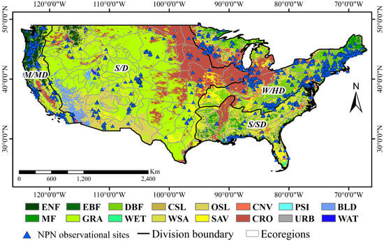
Figure 1.
The four ecological divisions used in this study superimposed on land cover types. The land cover types shown are Water (WAT), Permanent Snow and Ice (PSI), Evergreen Needleleaf Forest (ENF), Evergreen Broadleaf Forest (EBF), Deciduous Broadleaf Forest (DBF), Mixed Forest (MF), Closed Shrublands (CSL), Open Shrublands (OSL), Woodland Savanna (WSA), Savannas (SAV), Grasslands (GRA), Permanent Wetlands (WET), Croplands (CRO), Urban and Built-up (URB), Cropland/Natural Vegetation Mosaic (CNV), and Barren Land (BLD). The four ecological divisions are warm or hot continental division (W/HD), steppe or desert division (S/D), subtropical or savanna division (S/SD), and marine regime mountains or Mediterranean division (M/MD).
2.2. Data and Data-Processing
2.2.1. Ground-Based Observations of Spring Phenology and Meteorological Data
- (1)
- Ground-based spring phenology data
The ground-based spring phenology data employed in this study originated from the USA-NPN. The NPN maintains a network of volunteer phenology observers who amass comprehensive ground observations across the USA. The observers follow a standardized process of monitoring floral and faunal phenology and record data by intensity or abundance [35]. In the case of observations of single plant specimens, the observation site is considered to encompass only the immediate vicinity. However, if there are multiple adjacent specimens within very similar surroundings not exceeding an area of 15 acres (6 hectares), this area may also judiciously be deemed a single location.
This study drew upon ground phenological data acquired by the USA-NPN from 2016 to 2021. A compendium of 9953 phenological entries spanning the mainland United States and documenting an array of floral varieties was drawn on. Figure 1 depicts the extensive geographical coverage of the observation sites, which are distributed across diverse ecological zones. Certain phenological stages with similar definitions had been divided into multiple stages owing to variations between observed plant species. The resulting seventeen stages were consolidated into seven classes; these are described in Table 1. Two datasets provided by the NPN were used: individual observation records noting the onset of each phenological phase, and status and intensity reports that describe the phenology of individual plants and quantify the percentage prevalence of biological events.

Table 1.
Statistics related to ground observations of spring phenology and details of the consolidation of the seventeen original phenological stages into seven classes.
- (2)
- Meteorological data
The meteorological data used in this study, including temperature, precipitation, and surface shortwave radiation flux density data (referred to as radiation data), were obtained from the DaymetV4 (Daily Surface Weather and Climatological Summaries Version 4) project at the NASA ORNL DAAC data center at Oak Ridge National Laboratory [36]. This project, funded by the US Department of Energy, provides worldwide high-resolution daily meteorological data including precipitation, temperature, solar radiation, and vapor pressure data. It aims to further understanding in the fields of climate change, ecological science, agriculture, water resource governance, and Earth science. In this research, meteorological data for the desired locations were downloaded from the Google Earth Engine (GEE) platform. Based on earlier studies and personal experience, the pre-season was considered as extending from November 1st to the initiation of the SOS. The daily mean temperature during this period was defined as the pre-season average temperature (Tmean), the total rainfall as the pre-season cumulative precipitation (pre), and the aggregate solar radiation as the pre-season total radiation (srad). These metrics were employed in an investigation of the environmental determinants controlling the divergence between ground and remote observations of spring vegetation phenology.
2.2.2. Remote-Sensing Data
Advances in remote sensing have enhanced both the spatial and temporal resolutions of satellite instruments. Sentinel-2A launched in June 2015 originally provided free high-resolution optical imagery at resolutions of 10 to 60 m at 10-day intervals; this interval was reduced to 5 days when Sentinel-2A was joined by Sentinel-2B [37]. The diverse uses of Sentinel-2 include global vegetation phenology monitoring, surface hydrology observations, crop yield estimation and post-fire recovery assessment. Sentinel-2 has demonstrated immense potential in LSP research, particularly in the extraction of medium to high-resolution LSP [38,39]. The Normalized Difference Vegetation Index NDVI (NDVI) is widely employed for extracting information related to the growth and coverage of green vegetation as well as its biomass. Hence, in this study, we employed the NDVI to invert phenological variables from remote-sensing data. Within GEE, we applied quality control to the Sentinel-2 surface reflectance data to remove clouds, shadows, and aerosols. Following this, the NDVI was computed from the red and near-infrared band reflectance. The average NDVI values within 30-m squares centered on the observation sites were then calculated. The final output consisted of maximum NDVI by using the maximum value composite method values and times per site. However, due to the presence of noise, NDVI time-series often contain outliers and missing values, which makes it challenging to extract phenological transition points. To overcome these challenges and to improve the continuity and smoothness of the data and to make the seasonal vegetation signal clearer, it is common practice to perform data reconstruction and gap-filling. In this case, we employed the S–G filter (Savitzky–Golay filter) [40] to perform denoising of the time-series data. Then, the daily NDVI values were extracted by polynomial curve fitting (PCF) [37].
2.3. Methods
2.3.1. Retrieval of Spring Phenology from Remote-Sensing Data
The SOS metrics that were used were derived by calculating the average of dynamic thresholding (Equation (1)) and maximum slope analysis (Equation (2)). Dynamic thresholding, proposed by White et al. in 1997 [41], offers flexibility in selecting thresholds and has been successfully applied to various vegetation types at different latitudes [42]. The method takes into account the seasonal variation in vegetation index time-series, thus mitigating the influence of soil background values and vegetation types to some extent [43]. Maximum slope analysis assumes that the SOS is the point in time when the vegetation growth rate begins to increase rapidly. Based on this premise, this analysis involves calculating the derivative of the vegetation index time-series over the entire year. The date corresponding to the maximum rate of increase of the NDVI is then designated as the SOS [41]. As this method has fewer restraints, it is suitable for determining start and end dates of vegetation types for a wide range. The formulas are as follows:
where denotes the value at day , denotes the annual maximum value of at the site, denotes the minimum value of the that is the part of the curve corresponding to the period before the occurrence of , and denotes the value of when the original range of values is stretched to the range 0–1. In this study, the day corresponding to a of 0.5 was taken as the SOS identified by the dynamic thresholding method. The NDVI ratio of 0.5 is defined as the threshold for the start of spring, and note that the satellite-based green-up onset is described as the start of active vegetation growth, which is usually later than the time of first leaf unfolding or budburst [41]. denotes the slope at day , and denotes the value at day .
2.3.2. Scale Conversion of Ground-Based Observations of Spring Phenology
Ground-based phenology observations typically focus on small-scale objects such as individual plants or neighboring populations. In contrast, LSP is derived from remote-sensing imagery through a series of processing and inversion steps. As well as information about the target objects, remote-sensing imagery captures information about the surrounding vegetation or non-vegetated areas; this results in a scale effect between ground-based observations and the information derived from remote-sensing data. This phenomenon can introduce inaccuracies in LSP, and it is, therefore, common practice to upscale the ground observations to match the scale of the remote-sensing observations. One of the most commonly used methods is the mean ascending-scale aggregation method (Equation (3)), which involves calculating the average date for the beginning of a particular phenological stage for all species at a given site within a specific period:
Here, is the average date of the onset of the stage at the site, is the time of onset of the stage for species , and is the number of species recorded at the site.
2.3.3. Simulation of LUD
The ground-based LUD data used in this study were not based on continuous daily observations. Therefore, when exploring the association between LUD and remote sensing-derived phenology, there were cases where no ground-based data were available. Meanwhile, the Weibull distribution is considered an appropriate distribution for estimating phenology based on limited data. In this study, a new method for parameterizing the Weibull distribution to estimate phenology was employed to simulate the leaf-unfolding degree. This method incorporated bias rectification for random variable boundaries and based on the manual observation of vegetation leaf-unfolding on the ground, and it is applicable for estimating the timing of any percentile of leaf-unfolding. Cooke (1979) developed a bias-corrected estimation method for the boundaries of a random variable; the performance of this method outperforms many extreme value statistics [44] and utilizes a statistical framework to develop a numerical solution for computing point estimates of any percentile. This is shown in Figure 2, a workflow for the simulation of LUD by a Weibull-parameterized point estimator.
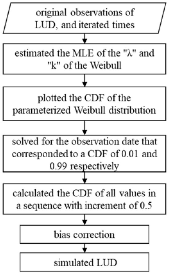
Figure 2.
Workflow for simulation of LUD.
To estimate arbitrary percentiles, the method employs the fitted integral to estimate the shape and scale parameters of the Weibull distribution using maximum likelihood estimation (MLE). After these parameters have been estimated, the cumulative distribution function (CDF) of the parameterized Weibull distribution is plotted. The CDF for the Weibull curve can be calculated as:
where is the observation, is the scale parameter, and is the shape parameter.
After obtaining the CDF of the Weibull distribution, the approximate bounds of the Weibull distribution parameterized by the original observations were computed by solving for for observation dates corresponding to CDF values of 0.01 and 0.99. For a CDF value of 0.01 this gave:
and for a value of 0.99 this gave:
In order to ensure that the CDF was smooth, further calculations were performed to determine the CDF values for all dates from the observation date corresponding to a CDF value of 0.01 until the date corresponding to a CDF of 0.99 in steps with a size of 0.5. This sequence of CDF values for each date produced a smoothed CDF curve, thus allowing for the simulation of observation dates corresponding to any percentile of the CDF. To simulate the dates corresponding to the LUD, the CDF curve of the Weibull distribution was constructed using the first date when the LUD exceeded 95% and the status and intensity data for each site.
3. Results
3.1. Relationship between Ground-Based Observations and Remote-Sensing Spring Phenology Retrievals
To ensure the reliability of the data and eliminate the influence of irrelevant information, this study removed data from ground-based phenology observations and SOS values greater than 200 (DOY) based on real-life experience and previous research findings. Additionally, after upscaling the ground-based phenology observations, data points with a time difference of more than 60 days between the upscaled values and SOS were removed.
As shown in Figure 3, a significant correlation was found between the ground-based phenological data and the SOS estimates derived from the Sentinel-2 data using the method described above. The values of R for the leaves, young leaves, and increasing leaf size stages are all greater than 0.6, with values of 0.653, 0.696, and 0.626, respectively. And the young leaves stage exhibited the highest RMSE of 38.661. Conversely, the all leaf buds broken stage had the lowest R value of 0.334 and the lowest RMSE of 24.345, and slightly lower than the emerging needles stage (R = 0.471) with an RMSE of 36.632. In comparison, the leaves stage and increasing leaf size stage showed relatively higher R values with 0.653 and 0.625, and relatively lower RMSE with values of 31.895 and 28.928, respectively, indicating a better alignment with the satellite-derived SOS than the other phenological stages.
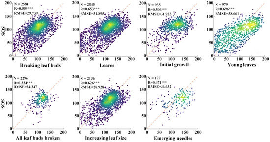
Figure 3.
Satellite-derived SOS dates plotted against ground-based phenological observations for the breaking leaf buds, leaves, initial growth, young leaves, all leaf buds broken, increasing leaf size, and emerging needles stages. ***: p < 0.001.
Furthermore, we compared the trends of ground-based observations and remote-sensing spring phenology during the leaves and increasing leaf size stages over the six years, as shown in Figure 4. It can be observed that the interannual variations of SOS and ground-based phenology exhibit a high level of consistency for these two growth stages.
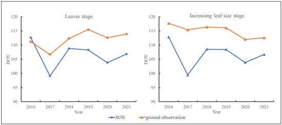
Figure 4.
Trends of ground-based observations and remote-sensing spring phenology from 2016 to 2021 for the leaves and increasing leaf size stages.
3.2. Remote Sensing of Spring Phenology Reflects the LUD
3.2.1. Variation in the LUD of Ground-Based and Remotely Sensed Spring Phenology
As has been demonstrated, the satellite-derived SOS results were most closely aligned with the dates of the leaves stage and increasing leaf size stage obtained from the ground-based observations. The status and intensity data for the increasing leaf size stage give the leaf area as a percentage of the area of the fully developed leaves; for leaves stage, these data indicate the proportion of leaves in the canopy. In order to examine the association between the satellite-derived SOS and ground-based observations of the LUD, status and intensity data for these two stages were obtained from the NPN. The correspondence between the SOS and different ranges of LUD was then investigated based on consideration of records for the same species at individual sites. It was found that, overall, the SOS corresponded most closely to ground LUD observations of 1–24%.
Figure 5a shows details of the correspondence between the increasing leaf size stage and the SOS. A leaf-unfolding degree of 1–24% was observed at 43.7% of all sites, the highest percentage shown. Sites with an LUD in the range 25–49% accounted for 20.31% of all sites. The number of sites with LUDs in the ranges 50–74%, 75–94%, and 95–100% are similar, comprising 11.93%, 10.43%, and 13.63% of all sites, respectively.
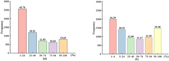
Figure 5.
Relationship between SOS and ground-based LUD for (a) the increasing leaf size stage and (b) the leaves stage for all pixels.
Figure 5b shows the correspondence between the leaves stage and the SOS. Sites with an LUD ranging from 1–4% represent 26.29% of all sites; sites with LUDs of 5–24% and 95–100% represent 18.53% and 19.38% of all sites, respectively. In this case, the number of sites with LUDs in the ranges 25–49%, 50–74%, and 75–94% are similar, comprising 12.09%, 11.17%, and 12.55% of all sites, respectively.
3.2.2. Relationship between Simulated LUD and Remotely Sensed Spring Phenology
The manual observations conducted by the USA-NPN can only determine the statue and intensity of the leaves stage and increasing leaf size stage within specific percentage ranges. It is not possible to determine the LUD with a precision of 1%. However, the Weibull distribution possesses characteristics that enable the prediction and determination of boundaries. Building upon this method and previous research, we developed a model to simulate the LUD during the leaves and increasing leaf size stages to a precision of 1%. To validate the accuracy of this model, the ground-based LUD data were compared with the data generated by the model. Samples with a matching rate of 60% or higher were then selected for further investigation of the relationship between the SOS and the simulated LUD data.
Figure 6a shows the mean absolute difference in days between the SOS and the corresponding simulated LUD. This difference first decreases up to an LUD of 12% then steadily increases. The standard deviation also decreases and then increases, with the minimum standard deviation being reached for an LUD of between 15% and 20%.
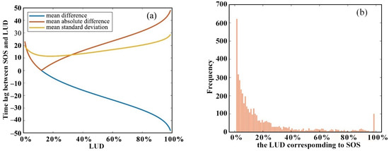
Figure 6.
(a) Difference between the SOS and the corresponding simulated LUD and (b) the frequency with which different values of the simulated LUD correspond to the SOS for all pixels.
In Figure 6b it is shown that pixels with LUDs of 1%, 2%, and 3% most frequently correspond to the SOS; there is also a sharp peak at an LUD of 99% (LUD99%). The minimum time difference between the SOS and the LUD occurs at LUD12% and LUD13%. Figure 7 shows the relationship between the SOS and the six most frequently occurring LUDs. The R2 values between the SOS and the LUD range from 0.65 to 0.81, with the highest correlation being observed at LUD13%. The RMSE values range from 9.58 to 14.96 days, with the lowest error occurring at LUD13%. The linear regression slope is largest and closest to 1 (0.972) at LUD2%. At LUD3%, LUD12%, and LUD13% the slope is just slightly less at around 0.96.
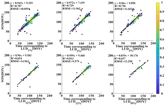
Figure 7.
Scatter plots showing the relationship between the SOS and the six most frequently occurring LUDs (1%, 2%, 3%, 12%, 13%, and 99%).
3.3. Environmental Factors Driving the Difference between Ground-Based Observations and Remote-Sensing Retrievals of Spring Vegetation Phenology
Due to the inconsistencies between ground-based observations of phenological development and satellite-derived SOS data at both spatial and temporal scales, as well as the differences in their definitions, the process of retrieving spring vegetation phenology introduces even greater discrepancies between SOS data and ground-based phenological observations. Therefore, an understanding of the environmental factors driving the differences between ground-based observations and SOS data is crucial to better comprehending the similarities and differences between these two phenological observation methods. This understanding has significant practical implications for verifying the authenticity and application of LSP data.
As described above, an LUD of 13% was found to correspond most closely to the SOS. In this section, details of our investigation of the influence of environmental factors on the difference in timing between SOS and LUD13% will be given. These environmental factors included the Tmean, pre and srad.
We first derived the difference between the SOS and the time of the occurrence of an LUD of 13% (SOS−LUD13%) for each species at each site and plotted this difference against the three factors listed above. Figure 8a shows a notable trend, with SOS−LUD13% increasing by 1.324 for every 1 °C increase in Tmean (R2 = 0.066). SOS−LUD13% has a range of −100 days to 100 days, with a concentration of points within the −40 to 20 days range, corresponding to a Tmean range of −2 °C to 8 °C. It is noticeable that, for a Tmean of below −2 °C, the majority of the SOS−LUD13% values are less than 20 days. As shown in Figure 8b, SOS−LUD13% also exhibits a positive correlation with pre—for every 100 mm increase in pre, SOS−LUD13% increases by 2.125 days (R2 = 0.046). The values of SOS−LUD13% are concentrated within the −40 to −20-day range, which corresponds to a range of 100−800 mm for pre. However, when pre exceeds 800 mm, most values of SOS−LUD13% lie within the range −60 to −40 days. Finally, as shown in Figure 8c, there is also a significant positive correlation between SOS−LUD13% and srad. For each 1 kW/m2 increase in srad, there is an increase of 1.413 days in SOS−LUD13% (R2 = 0.328).
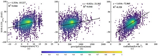
Figure 8.
Scatter plot of SOS−LUD13% against the environmental factors (a) pre-season mean temperature, (b) pre-season cumulative precipitation, and (c) pre-season cumulative radiation.
Most previous studies have already indicated a strong phenological differentiation between tree species populations [45,46]. Different species exhibit significant variations in leaf-unfolding phenology, and even within the same species, the timing of leaf unfolding can differ across different habitats. We selected the nine most representative species to compare the Pearson correlation coefficients for the relationship between SOS–LUD13% and Tmean, pre, and srad. The results are presented in Table 2. Overall, except for American beech, SOS−LUD13% shows a significant correlation with all three environmental factors for the different species, with rad exhibiting a slightly stronger correlation than the other two factors. Regarding the correlation between SOS–LUD13% and Tmean, with the exception of black cherry, for which the correlation coefficient is relatively low (0.176), the correlation coefficients are between 0.2 and 0.5. In terms of the correlation between SOS–LUD13% and pre, except for sugar maple, which has a low correlation coefficient (0.198), and for American Beech, for which there is no significant relationship, the correlation coefficients are between 0.3 and 0.6. Finally, for the relationship between SOS–LUD13% and srad, Florida privet and Lagerstroemia speciosa have the highest correlation coefficients (0.843 and 0.844, respectively); the other species have coefficients of approximately 0.6 to 0.8.
Table 2.
Correlation between SOS–LUD13% and environmental factors for different species.
We also calculated the Pearson correlation coefficients for the relationships between SOS–LUD13% and the environmental factors for the four ecological regions—M/MD, S/D, S/SD, and W/HD—defined earlier. As shown in Table 3, except for the S/D region, for which there is no significant correlation between SOS–LUD13% and pre, there are significant correlations between SOS–LUD13% and all three environmental factors. Furthermore, in all four regions, the correlation between SOS–LUD13% and srad has a coefficient of above 0.4—higher than for pre and Tmean in each case. For Tmean, the M/MD and S/D regions have relatively low coefficients of 0.169 and 0.1884, respectively. For S/SD and W/HD, this coefficient is slightly higher at 0.259 and 0.366, respectively. For the S/D region, there is no significant correlation between SOS–LUD13% and pre; however, the other three regions have coefficients of between 0.2 and 0.4 for this relationship. For srad, in the M/MD and S/D regions, the correlation coefficients for the relationship with SOS–LUD13% are in the range 0.4 to 0.6, and for the S/SD and W/HD regions they are between 0.6 and 0.7.
Table 3.
Correlation between SOS-LUD13% and environmental factors for different ecological zones.
4. Discussion
4.1. The Significant Correlation between the Leaves and Increasing Leaf Size Stages and the SOS
Ground-based observations of vegetation phenology data provide important validation data for assessing phenology metrics obtained by inverting remote-sensing data. Previously, ground observations were mainly used to make coarse spatial resolution assessments at ecosystem scales [47,48,49]. In this study, it was found that the onset of ground-based phenological stages at each site, as obtained using the mean ascending-scale aggregation method, was significantly correlated with the SOS derived from Sentinel-2 data. In particular, the SOS was found to be closely correlated with the leaves and increasing leaf size stages. Furthermore, the simulation based on the Weibull distribution model indicated that an LUD of 13% corresponded most closely to the SOS. The sharp increases in vegetation index values in spring are closely related to leaf unfolding and is associated with an increase in the leaf area index and chlorophyll concentration [50]. In the study by Bórnez et al. [51], it was found that for deciduous broadleaf forests in Europe and the United States, the RMSE between ground-based observations of the increasing leaf size and leaves stages and the satellite-derived SOS was 9 days and 11 days, respectively. During the leaves stage, the entire leaf structure emerges from the leaf buds, and the expanded leaves become visible. Both the leaf area and chlorophyll concentration increase during this stage. The remote-sensing index, NDVI, shows a significant increase during this phase, and it is commonly accepted that ground-based observations of the leaves stage correspond to the remote sensing-derived SOS. Studies have found a significant positive correlation between the remotely sensed SOS and the leaves stage, with the highest correlation being observed for broadleaf forests in the eastern United States [17]. White et al., conducted a study comparing the relationship between the SOS and ground-based observations of phenological stages in North America. These results also indicated a significant correlation between the SOS and ground-based determination of the leaves stage [16]. Additionally, Luo et al., conducted research in northern China, comparing four tree species, and found that the remotely sensed SOS extracted from GIMMS NDVI3g data was highly consistent with ground-based observations during the leaves stage [52]. During the increasing leaf size stage, most leaves on the plants have not yet reached their full size and continue to grow. It is known that the leaf area continues to expand during this stage, resulting in a noticeable increase in the NDVI. Liang et al., found that there was consistency between the SOS and the duration of the increasing leaf size stage as determined by ground observations [53]. Together, these studies confirm the high level of agreement between the occurrence of the SOS, the leaves stage, and the duration of the increasing leaf size stage. The findings of the current study are thus in line with the existing literature, further confirming the reliability of the results.
4.2. Variations in the Relationship between the LUD and SOS between Species
The phenology of plants is influenced by their genetic characteristics, as different species possess distinct biological clocks and growth habits, resulting in variations in their lifecycles. For instance, early spring flowering plants may be influenced by factors such as temperature and sunlight, whereas plants that bloom in the summer can be affected by rainfall and temperature. Even when exposed to the same conditions, there can be considerable differences in spring phenology between plants of the same type [54,55]. Different deciduous broadleaf tree species exhibit differences in leaf-fall and budburst timing [56]. Inter-specific differences in spring phenology are also believed to be strongly influenced by varying species-specific requirements for warming and chilling, as well as differences in sensitivity to abiotic drivers [57]. For example, the sensitivity to spring temperature differs significantly between oka and beech, with budburst advancing by 7.26 days and 2.03 days, respectively, for every 1 °C increase in temperature [58]. Previous research has shown that the vegetation phenology of different species exhibits different temperature sensitivities and that this can lead to either the compression or extension of growing seasons [59,60,61]. Plant species with earlier leaf-unfolding times tend to have a higher temperature sensitivity, enabling them to initiate growth earlier and gain a competitive advantage in interspecific competition as spring temperatures rise.
The physiological structures, morphological characteristics, and environmental adaptability of plant species vary greatly with ecological type. Previous studies have shown that the consistency between remote-sensing and ground-based phenology varies depending on the species and vegetation type [62,63,64], and the findings of this study are consistent with previous research. We selected species from the W/HD ecological region with sample sizes exceeding 30 to investigate the variations in the differences between the SOS and the corresponding occurrence of the LUD at different simulated LUDs for different species within the same ecological zone. The results are shown in Figure 9. The results indicate that there are differences in the LUD that correspond to the minimum difference between the SOS and the simulated LUD for different species. For red maple, the smallest difference occurs at LUD16%, for platanus orientalis, this occurs at LUD29%, for Northern quercus rubra, it occurs at LUD13%, for sugar maple, the smallest difference occurs at LUD11%, for Florida privet, it occurs at LUD19%, and for black cherry, it occurs at LUD27%.
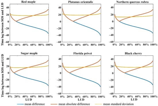
Figure 9.
Difference between the SOS of major species in the W/HD ecoregion and the date corresponding to the simulated LUD. The species investigated were red maple, platanus orientalis, Northern quercus rubra, sugar maple, Florida privet, and black cherry.
Temporal variations in vegetation phenology and physiological variables are highly heterogeneous in space, within species, and between species [21,65]. Within the same plant community, different species may employ distinct strategies to cope with climate change, and numerous factors contribute to variations in the timing of leaf unfolding for plants of both the same and of different species. These include environmental factors such as temperature, humidity, rainfall, and CO2 concentration [66] as well as the genetic characteristics of the different species themselves [67]. Influencing biotic factors include insects and fungi [68], tree height, and canopy density. Furthermore, not all species respond to the same driving factors, such as spring temperature increase, at the same rate [56,69,70,71]. In this study, we focused on nine representative species and calculated the relevant Pearson correlation for each species to investigate the factors driving the phenology of different species (Table 4 and Table 5).
Table 4.
Correlation between LUD13% and climatic factors for different species.
Table 5.
Correlation between SOS and climatic factors for different species.
The above results reveal that there are variations in the response of LUD13% and SOS to the changes in the three environmental factors between the nine representative species. For LUD13%, for all species, the highest correlation is with Tmean—the correlation is negative in all cases. The strongest correlation of all is for fragrant sumac, which has a correlation coefficient of −0.801; American beech (−0.799) and red maple (−0.771) follow closely. For the other species such as Florida privet, black cherry, and sugar maple, the absolute value of the correlation coefficient is in the range 0.4 to 0.6. However, while the SOS shows a negative correlation with Tmean, there are also species whose SOS exhibits a positive correlation with Tmean. The SOS of five species—red maple, black cherry, sugar maple, American beech, and fragrant sumac — is significantly negatively correlated with Tmean, with correlation coefficients ranging from −0.48 to −0.13. In contrast, the SOS of lagerstroemia speciosa shows a significant positive correlation with Tmean, with a correlation coefficient of 0.246. Overall, for SOS, the most significant positive correlation is with srad, with all the correlation coefficients exceeding 0.8. For most species, the correlation coefficients between the time of occurrence of LUD13% and srad range from around 0.2 to 0.4, with the value for white oak being just under 0.2. For all species, the SOS shows a significant positive correlation with pre, with correlation coefficients ranging from 0.3 to 0.5. These findings suggest that there are notable differences in the response of LUD13% and remote sensing-derived phenology to different climate conditions.
4.3. Influence of the Ecological Zone on the Correlation between the LUD and SOS
Plant phenology is not only influenced by the species, but also by the growth environment, as plants respond to environmental factors by adjusting the timing of their leaves, leaf senescence, and flowering stages [72,73,74]. The growth of plants relies on external environmental factors such as the temperature, as well as the availability of nutrients, water, and light; these factors vary between ecological regions and provide varying conditions for plant growth. Consequently, plants may exhibit different phenological patterns in different regions. Furthermore, there are genetic differences between the phenological responses of populations growing under different climatic conditions [75]. Studies have shown that the degree of spring leaf unfolding is influenced by the interaction between nutrient availability and soil moisture, and that the earlier occurrence of spring phenological phases exhibits regional and interspecies variations [76,77]. Within a plant community, the responses of canopy trees, understory shrubs, and herbaceous plants to changes in the growth environment can affect the competition for water and soil nutrients between these functional groups [75].
There are significant differences in leaf unfolding phenology between plant species, and even within the same species, there are differences in the timing of leaf unfolding in different habitats [56,78,79]. The findings of our study confirm these observations. We calculated the proportion of sites where the SOS corresponds to the LUD at the leaves stage for the same species in different ecological regions (Figure 10). The results indicate that for red maple, the ratio of the LUD to SOS in the W/HD and S/SD regions is similar. For fragrant sumac, this ratio of the LUD between 1% and 4% is slightly higher in the S/SD ecological region than in the W/HD ecological region, and the proportion of sites with an LUD of above 95% is also slightly higher in the S/SD region. For privet, in the S/SD ecological region, the ratio of the LUD to SOS is slightly higher than in the W/HD ecological region for an LUD between 1% and 4% but slightly lower for an LUD above 95%. For black willow, the ratio of the LUD between 1% and 4% to SOS is significantly lower in the S/D ecological region than in the W/HD region. In addition, the proportion of sites with an LUD of between 25% and 49% is lower in in the S/D ecological region than in the W/HD region but the proportion of sites with an LUD in the range 50–74% is significantly higher. For trembling willow, there is significant variation in the ratio of the LUD to SOS across the W/HD, S/D, and M/MD ecological regions. The lowest ratio (1–4%) occurs in the S/D ecological region, and the highest value occurs in the M/MD region. Furthermore, in the S/D ecological region, the proportion of sites with an LUD between 75% and 94% or above 95% is greater than in the other two ecological regions.
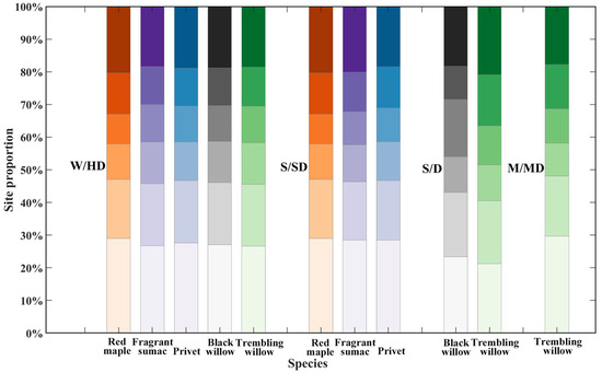
Figure 10.
Proportion of sites where the SOS corresponds to the LUD at the leaves stage in different ecological zones.
We also calculated the difference between the SOS and the corresponding LUD time for all species within the four ecological zones, as shown in Figure 11. We found that there are differences in the LUD that corresponds to the minimum time difference between the SOS and simulated LUD between the different regions. In M/MD, the smallest difference is observed at LUD10%, whereas in S/D, the smallest difference occurs at LUD22%, and in S/SD, the smallest difference is observed at LUD20%. In the W/HD ecological zone, the smallest difference occurs at LUD12%. Notably, the standard deviation in the W/HD ecological zone remains at around 20 days and exhibits minimal variation as the LUD increases.
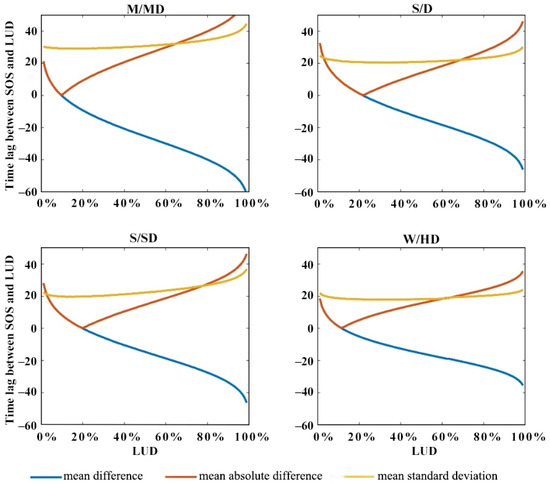
Figure 11.
Difference between the SOS and simulated LUD in the M/MD, S/D, S/SD, and W/HD ecoregions.
Different species exhibit varying degrees and even directions of response to environmental changes, and these differences also vary with the location. Research indicates that, over the past 40 years, the onset of leaf unfolding in temperate tree species has become significantly earlier, a trend that has been attributed to climate warming. Studies of long-term temperature sensitivity and the factors influencing spring plants have revealed a significant positive correlation between the reproductive phase of most species and temperature [80]. Other studies conducted using modeling and remote sensing in temperate forests have also indicated that the spring leaves stage has advanced in recent decades (at a rate of 1.8–7.8 days per decade) although there are variations between species. In high-altitude and high-latitude regions, the amount of snow accumulation and the time when snow-melt occurs are two key additional factors that influence plant phenology [81]. The availability of water can also influence phenology in temperate and boreal forests—but to a lesser extent than temperature [82]. Changes in water availability can lead to complex phenological changes and may have profound effects on ecosystem functionality and structure. Dry and wet tropical climates are distinguished by the amount of precipitation and its seasonal variation, and differences in community phenology levels are often driven by the duration of the dry season [83]. Previous studies have confirmed that, in tropical regions, temperature, precipitation, and radiation can interact and have complex effects on plant phenology [84,85,86]. In addition to being constrained by water stress, the leaf unfolding time in tropical forests is also correlated with the annual peak radiation [83]. Solar radiation (total sunshine duration, peak radiation, or photoperiod) is also considered a primary driving factor of tropical phenology [87]. In most tropical grassland areas, precipitation is a driving factor of plant phenology, and the inverse relationship between radiation and phenology is consistent with the inhibition of grassland growth due to soil moisture limitations [87]. Temperature is a key driving factor for most species, but precipitation, through its influence on soil moisture, is also important in many cases [88]. Summer drought resulting from low precipitation is a typical characteristic of Mediterranean ecosystems, and the seasonal variation in water availability controls vegetation activity, with most plant growth occurring during the colder but wetter times of the year [89,90]. In semiarid and arid desert ecosystems, phenological changes resulting from climate change can be driven by both the timing and amount of precipitation, as well as the increase in temperature. Water availability appears to be a key driver of phenology in arid and semiarid ecosystems [91], whereas temperature and humidity are the primary drivers of phenology in grassland ecosystems [24].
To investigate the driving factors of phenology in different ecological regions, specifically temperature, precipitation, and radiation, we calculated the Pearson correlation coefficients between both the timing of LUD13% and SOS and these three environmental factors in the M/MD, S/D, S/SD, and W/HD ecological regions (Table 6 and Table 7).
Table 6.
Correlation between LUD13% and environmental factors in different ecological zones.
Table 7.
Correlation between SOS and environmental factors in different ecological zones.
Table 6 reveals significant negative correlations between the timing of LUD13% and Tmean in all four ecological regions. In some cases, there is a significant positive correlation with pre. For all four regions, the correlation coefficient between the timing of LUD13% and Tmean is around −0.5. It is notable that the M/MD and S/SD ecological regions have similar correlation coefficients (−0.539 and −0.534, respectively) that are slightly higher than those of the other two regions. The lowest correlation occurs in the S/D region. In both the M/MD and S/D ecological regions, there is a significant correlation between the timing of LUD13% and pre—the correlation coefficients are 0.162 and 0.207, respectively. In all four regions, the relationship between the timing of LUD13% and srad is close to or slightly below 0.2 and is lowest in the M/MD region (0.145). Notably, in the M/MD and S/D regions, the timing of LUD13% is significantly correlated with all three environmental variables, whereas in the S/SD and W/HD regions, there is only an association with Tmean and srad.
Table 7 indicates that there are significant correlations between the remotely sensed vegetation phenology and Tmean, pre, and srad in all four ecological regions. The correlation with srad was found to be higher than that with Tmean and pre. In all four regions, the correlation with Tmean is significantly negative: the M/MD region has the strongest negative correlation, with a coefficient of −0.337; this is followed by the S/D region with a coefficient of −0.278, then the S/SD ecological region with a coefficient of −0.229, and finally the W/HD ecological region with a coefficient of only −0.033. In contrast, in all four regions, the SOS shows a significant positive correlation with pre. The M/MD ecological region has the highest correlation with a coefficient of 0.513, and the S/D region has the lowest correlation with a coefficient of 0.261. The S/SD and W/HD regions have similar correlation coefficients of 0.366 and 0.368, respectively. In all four regions, the SOS also shows a significant positive correlation with srad. The M/MD region has the lowest correlation with a coefficient of 0.681, whereas in the S/D ecological region the correlation coefficient is 0.812. The S/SD and W/HD regions have similar correlation coefficients of 0.91 and 0.922, respectively.
4.4. Effects of Vegetation Phenology Monitoring and Modeling on the Relationship between LUD and SOS
Because of the proven reliability of vegetation spring phenology monitoring using remote-sensing indices such as the NDVI and the Enhanced Vegetation Index (EVI), particularly as applied to large geographical areas [4,13,92,93,94], this type of monitoring has become widely used in recent years. However, it is important to acknowledge that the processes of leaf unfolding and leaf-fall occur gradually over large geographical areas. Consequently, these remote-sensing data products have certain limitations in terms of continuous observations of phenology, which leads to a lag in the detection of vegetation changes. Furthermore, there are inherent differences in the quality of information obtained from ground-based phenological observations and remote-sensing retrievals, which leads to discrepancies between them [95,96].
Firstly, remote-sensing observations of forests are made from a zenithal angle, capturing signals from the top of the canopy, whereas ground-based observations collected by field technicians focus on the bottom of the canopy; this results in potential discrepancies between the phenological information obtained by the two methods. To date, most studies use indirect methods to identify phenology variation based on the time series of PhenoCam images. PhenoCam involves mounting digital cameras with visible-wavelength imaging sensors above vegetation canopies to capture images throughout the day [97]. Near-surface observations from PhenoCam provide time series of images that are ideal for tracking seasonal changes in leaf phenology, and have been used to extract leaf phenology metrics [98] and track biodiversity [99]. The current studies have proven that PhenoCam images carry useful information for monitoring and understanding leaf phenology. Secondly, LSP and ground-based observations are concerned with different characteristics [95]. Ground-based observations target individual plants or species at a specific scale, while remote sensing provides aggregated information related to vegetation growth at the pixel scale [19]. Since image pixels often contain multiple land cover types or species, the presence of heterogeneous vegetation cover can introduce errors in phenological dates obtained from remote-sensing data, as compared with ground-based observations. In addition, the pixels neighboring the pixel of interest can influence the signal received by the satellite, as the ground area corresponding to the analyzed pixel may not entirely correspond to the actual area contributing to the detected signal [100]. Zhang [101] also noted that the extraction of SOS results at coarse resolutions is predominantly determined by pixels where the SOS occurs earlier. However, there are also uncertainties inherent in ground-based phenological observations. For example, the phenological data collection strategy employed by the USA-NPN requires field technicians to monitor the occurrence, duration, and intensity of key phenological events and record them in discrete categories that may not fully capture the gradual transitions in leaf phenology. The Weibull distribution is increasingly used to estimate the dates of hard-to-observe phenological events, such as first and last flowering dates [102,103]. These contrasting results occur because of sampling biases in the raw data, which the statistical estimator corrects by providing estimates for the true statistical data. However, estimating the true onset or offset of a process may be more challenging than estimating a percentile of the phenology curve within the bounds, because it is notoriously difficult to model the tails of distributions as there are fewer data points to parameterize the model [103]. Finally, there is no universally applicable algorithm for phenological parameter extraction [104]. The threshold method used for SOS extraction is simple and effective, and it is widely used. However, it is subject to significant subjective factors (such as the different thresholds provided by different researchers, which can lead to noticeable variations in the length of the growing season) and does not fully take into account environmental influences (such as differences in the soil background and vegetation type) [105]. Researchers have confirmed that the consistency between LSP and ground-based phenology varies depending on the species or vegetation type [62,64,106]. On the other hand, the derivative method, although threshold-free and biologically meaningful, is more sensitive to data noise, requiring higher smoothness requirements at the data preprocessing stage [107]. Additionally, in cases where the vegetation index curve does not exhibit abrupt changes, determining the start and end dates of the growing season becomes challenging, particularly when there is cloud contamination in the time series data of the vegetation index. The retrieval of phenology using remote sensing offers the advantage of broad spatial coverage; however, the results are influenced by various factors, including atmospheric disturbances, solar radiation effects, cloud cover, and the duration of snow cover [108]. This limits the capability of remote-sensing data to capture species-specific phenological information.
The process of monitoring LSP is strongly influenced by ecosystem processes and vegetation types [16,109,110,111]. Previous studies have shown that LSP estimation is most reliable in deciduous forests but becomes challenging in evergreen forests [109,110,112,113,114,115]. We analyzed the relationship between ground-based observations and remote-sensing spring phenology retrievals at the species and ecological region levels. However, due to limitations in the available data, the species composition was relatively homogeneous, with a predominance of deciduous broadleaf species. Consequently, we did not specifically analyze the relationship between ground-based observations and the remotely sensed phenology for different vegetation types. To improve the comparability and spatiotemporal consistency of phenological parameter results obtained from different regions and time periods, further research needs to be done to develop universally applicable phenological extraction algorithms. Additionally, while this study examined the relationship between ground-based observations, remote-sensing retrievals of vegetation spring phenology, and the associated environmental driving factors under different conditions, a model that can convert ground-based observations to remotely sensed spring phenology data still needs to be developed. Future research should address this gap to enable the application of the findings from this study to the validation of remote-sensing retrievals of vegetation spring phenology. This will allow more accurate information relating to plant phenology and leaf unfolding to be obtained using remote-sensing data.
5. Conclusions
In examining the relationship between ground-based observations and the SOS, it is common to use the start time of a specific phenophase as the ground-based observation, and ecological regions are often not systematically categorized to study the impacts of environment and species. This article examines the relationship between ground-based observations of the phenological stages of vegetation and the SOS. It distinguishes between ecological zones and species, and uses data from both the USA-NPN and Sentinel-2 satellite imagery. At the same time, the ground-based phenological stages were refined to the leaf-unfolding degree scale, and the association between the LUD and SOS was investigated. Then, by employing the Weibull distribution method, the LUD was quantified to a precision of 1%, which enabled the exploration of the relationship between simulated values of the LUD and the SOS. A study of the environmental factors that affect the relationship between the SOS and LUD was also conducted. Our investigation concluded that there was a significant correlation between ground-based observations of spring phenology and the phenological data derived from remote-sensing data, particularly for the leaves and leaf-expansion stages. For the largest proportion of observation sites, the SOS corresponded to an LUD of 1% to 24%, with the strongest correlation and smallest error being for LUD13%. The consistency between the remotely sensing and ground-based spring phenology results depended on the species and ecological environment. However, in different species and ecological regions, LUD13%, SOS, and SOS−LUD13% all have a high correlation with pre-season cumulative radiation. This study provides a theoretical basis for selecting appropriate ground-based observation data to validate the authenticity of LSP.
Author Contributions
Conceptualization, J.X. and D.P.; Data curation, J.X., X.F., K.Y., Z.L. and D.P.; Formal analysis, J.X. and D.P.; Funding acquisition, J.X. and D.P.; Investigation, J.X., T.W., X.F. and D.P.; Methodology, J.X., T.W. and X.Z.; Project administration, D.P.; Resources, D.P.; Software, J.X. and X.F.; Supervision, D.P.; Validation, J.X., T.W. and D.P.; Visualization, J.X., T.W., X.F. and D.P.; Writing—original draft, J.X., T.W. and D.P.; Writing—review and editing, J.X., T.W., X.F., X.Z., K.Y., Z.L. and D.P. All authors have read and agreed to the published version of the manuscript.
Funding
This research was funded by the National Natural Science Foundation of China (42071329), Zhejiang Provincial Natural Science Foundation (Basic Public Welfare Research Project of Zhejiang Province) of China (LGF22D010008) and Science and Disruptive Technology Program, AIRCAS (2024-AIRCAS-SDPT-15, E2Z218020F).
Data Availability Statement
The data that support the findings of this study are available from the corresponding authors upon request.
Acknowledgments
The authors acknowledge the ground-observed spring vegetation phenology metrics were provided by the USA National Phenology Network.
Conflicts of Interest
The authors declare no conflicts of interest.
References
- Lieth, H. Purposes of a Phenology Book. In Phenology and Seasonality Modeling; Lieth, H., Ed.; Springer: Berlin/Heidelberg, Germany, 1974; pp. 3–19. [Google Scholar]
- Huang, P.; Zheng, X.; Li, X.; Hu, K.; Zhou, Z. More complex interactions: Continuing progress in understanding the dynamics of regional climate change under a warming climate. Innovation 2023, 4, 100398. [Google Scholar] [CrossRef]
- Piao, S.; Liu, Q.; Chen, A.; Janssens, I.A.; Fu, Y.; Dai, J.; Liu, L.; Lian, X.; Shen, M.; Zhu, X. Plant phenology and global climate change: Current progresses and challenges. Glob. Chang. Biol. 2019, 25, 1922–1940. [Google Scholar] [CrossRef] [PubMed]
- Stöckli, R.; Vidale, P.L. European plant phenology and climate as seen in a 20-year AVHRR land-surface parameter dataset. Int. J. Remote Sens. 2004, 25, 3303–3330. [Google Scholar] [CrossRef]
- de Beurs, K.M.; Henebry, G.M. Land surface phenology, climatic variation, and institutional change: Analyzing agricultural land cover change in Kazakhstan. Remote Sens. Environ. 2004, 89, 497–509. [Google Scholar] [CrossRef]
- Garonna, I.; de Jong, R.; Schaepman, M.E. Variability and evolution of global land surface phenology over the past three decades (1982–2012). Glob. Chang. Biol. 2016, 22, 1456–1468. [Google Scholar] [CrossRef] [PubMed]
- Julien, Y.; Sobrino, J.A. Global land surface phenology trends from GIMMS database. Int. J. Remote Sens. 2009, 30, 3495–3513. [Google Scholar] [CrossRef]
- Dai, W.; Jin, H.; Zhang, Y.; Zhou, Z.; Liu, T. Advances in plant phenology. Acta Ecol. Sin. 2020, 40, 6705–6719. [Google Scholar]
- de Beurs, K.M.; Henebry, G.M. Spatio-Temporal Statistical Methods for Modelling Land Surface Phenology. In Phenological Research: Methods for Environmental and Climate Change Analysis; Hudson, I.L., Keatley, M.R., Eds.; Springer: Dordrecht, The Netherlands, 2010; pp. 177–208. [Google Scholar]
- Pinzon, J.E.; Tucker, C.J. A Non-Stationary 1981–2012 AVHRR NDVI 3g Time Series. Remote Sens. 2014, 6, 6929–6960. [Google Scholar] [CrossRef]
- Schwartz, M.D. Monitoring global change with phenology: The case of the spring green wave. Int. J. Biometeorol. 1994, 38, 18–22. [Google Scholar] [CrossRef]
- Tucker, C.J. Red and photographic infrared linear combinations for monitoring vegetation. Remote Sens. Environ. 1979, 8, 127–150. [Google Scholar] [CrossRef]
- Zhang, X.; Friedl, M.A.; Schaaf, C.B.; Strahler, A.H.; Hodges, J.C.F.; Gao, F.; Reed, B.C.; Huete, A. Monitoring vegetation phenology using MODIS. Remote Sens. Environ. 2003, 84, 471–475. [Google Scholar] [CrossRef]
- Zhang, X.; Friedl, M.A.; Tan, B.; Goldberg, M.D.; Yu, Y. Long-term detection of global vegetation phenology from satellite instruments. Phenol. Clim. Chang. 2012, 16, 297–320. [Google Scholar]
- Wang, J.; Dong, J.; Liu, J.; Huang, M.; Li, G.; Running, S.W.; Smith, W.K.; Harris, W.; Saigusa, N.; Kondo, H. Comparison of gross primary productivity derived from GIMMS NDVI3g, GIMMS, and MODIS in Southeast Asia. Remote Sens. 2014, 6, 2108–2133. [Google Scholar] [CrossRef]
- White, M.A.; de Beurs, K.M.; Didan, K.; Inouye, D.W.; Richardson, A.D.; Jensen, O.P.; O’Keefe, J.; Zhang, G.; Nemani, R.R.; van Leeuwen, W.J. Intercomparison, interpretation, and assessment of spring phenology in North America estimated from remote sensing for 1982–2006. Glob. Chang. Biol. 2009, 15, 2335–2359. [Google Scholar] [CrossRef]
- Schwartz, M.D.; Reed, B.C. Surface phenology and satellite sensor-derived onset of greenness: An initial comparison. Int. J. Remote Sens. 1999, 20, 3451–3457. [Google Scholar] [CrossRef]
- Minyu, W.; Yi, L.; Zhengyang, Z.; Qiaoyun, X.; Xiaodan, W.; Xuanlong, M. Recent advances in remote sensing of vegetation phenology: Retrieval algorithm and validation strategy. Natl. Remote Sens. Bull. 2022, 26, 431–455. [Google Scholar]
- Morisette, J.T.; Richardson, A.D.; Knapp, A.K.; Fisher, J.I.; Graham, E.A.; Abatzoglou, J.; Wilson, B.E.; Breshears, D.D.; Henebry, G.M.; Hanes, J.M.; et al. Tracking the rhythm of the seasons in the face of global change: Phenological research in the 21st century. Front. Ecol. Environ. 2009, 7, 253–260. [Google Scholar] [CrossRef]
- Peng, D.; Zhang, X.; Zhang, B.; Liu, L.; Liu, X.; Huete, A.R.; Huang, W.; Wang, S.; Luo, S.; Zhang, X.; et al. Scaling effects on spring phenology detections from MODIS data at multiple spatial resolutions over the contiguous United States. ISPRS-J. Photogramm. Remote Sens. 2017, 132, 185–198. [Google Scholar] [CrossRef]
- Richardson, A.D.; Bailey, A.S.; Denny, E.G.; Martin, C.W.; O’Keefe, J. Phenology of a northern hardwood forest canopy. Glob. Chang. Biol. 2006, 12, 1174–1188. [Google Scholar] [CrossRef]
- Vitasse, Y.; Francois, C.; Delpierre, N.; Dufrêne, E.; Kremer, A.; Chuine, I.; Delzon, S. Assessing the effects of climate change on the phenology of European temperate trees. Agric. For. Meteorol. 2011, 151, 969–980. [Google Scholar] [CrossRef]
- Saleska, S.R.; Didan, K.; Huete, A.R.; Da Rocha, H.R. Amazon forests green-up during 2005 drought. Science 2007, 318, 612. [Google Scholar] [CrossRef] [PubMed]
- Craine, J.M.; Wolkovich, E.M.; Gene Towne, E.; Kembel, S.W. Flowering phenology as a functional trait in a tallgrass prairie. New Phytol. 2012, 193, 673–682. [Google Scholar] [CrossRef] [PubMed]
- Shen, M.; Piao, S.; Cong, N.; Zhang, G.; Jassens, I.A. Precipitation impacts on vegetation spring phenology on the T ibetan P lateau. Glob. Chang. Biol. 2015, 21, 3647–3656. [Google Scholar] [CrossRef] [PubMed]
- Fu, Y.H.; Piao, S.; Zhao, H.; Jeong, S.J.; Wang, X.; Vitasse, Y.; Ciais, P.; Janssens, I.A. Unexpected role of winter precipitation in determining heat requirement for spring vegetation green-up at northern middle and high latitudes. Glob. Chang. Biol. 2014, 20, 3743–3755. [Google Scholar] [CrossRef] [PubMed]
- Tang, J.; Körner, C.; Muraoka, H.; Piao, S.; Shen, M.; Thackeray, S.J.; Yang, X. Emerging opportunities and challenges in phenology: A review. Ecosphere 2016, 7, e01436. [Google Scholar] [CrossRef]
- Delbart, N.; Beaubien, E.; Kergoat, L.; Le Toan, T. Comparing land surface phenology with leafing and flowering observations from the PlantWatch citizen network. Remote Sens. Environ. 2015, 160, 273–280. [Google Scholar] [CrossRef]
- Ganguly, S.; Friedl, M.A.; Tan, B.; Zhang, X.; Verma, M. Land surface phenology from MODIS: Characterization of the Collection 5 global land cover dynamics product. Remote Sens. Environ. 2010, 114, 1805–1816. [Google Scholar] [CrossRef]
- Peng, D.; Zhang, X.; Wu, C.; Huang, W.; Gonsamo, A.; Huete, A.R.; Didan, K.; Tan, B.; Liu, X.; Zhang, B. Intercomparison and evaluation of spring phenology products using National Phenology Network and AmeriFlux observations in the contiguous United States. Agric. For. Meteorol. 2017, 242, 33–46. [Google Scholar] [CrossRef]
- Browning, M.; Lee, K. Within what distance does “greenness” best predict physical health? A systematic review of articles with GIS buffer analyses across the lifespan. Int. J. Environ. Res. Public Health 2017, 14, 675. [Google Scholar] [CrossRef]
- Bailey, R.G. Description of the Ecoregions of the United States; US Department of Agriculture, Forest Service: Washington, DC, USA, 1995. [Google Scholar]
- Bailey, J.P.; Bakos, Y. An exploratory study of the emerging role of electronic intermediaries. Int. J. Electron. Commer. 1997, 1, 7–20. [Google Scholar] [CrossRef]
- MacKenzie, D.I.; Bailey, L.L. Assessing the fit of site-occupancy models. J. Agric. Biol. Environ. Stat. 2004, 9, 300–318. [Google Scholar] [CrossRef]
- Rosemartin, A.H.; Denny, E.G.; Gerst, K.L.; Marsh, R.L.; Posthumus, E.E.; Crimmins, T.M.; Weltzin, J. USA National Phenology Network Observational Data Documentation; US Geological Survey: Washington, DC, USA, 2018. [Google Scholar]
- Thornton, M.M.; Shrestha, R.; Wei, Y.; Thornton, P.E.; Kao, S.; Wilson, B.E. Daymet: Daily Surface Weather Data on a 1-km Grid for North America, Version 4; ORNL DAAC: Oak Ridge, TN, USA, 1840. [Google Scholar]
- Vrieling, A.; De Leeuw, J.; Said, M.Y. Length of growing period over Africa: Variability and trends from 30 years of NDVI time series. Remote Sens. 2013, 5, 982–1000. [Google Scholar] [CrossRef]
- Jönsson, P.; Cai, Z.; Melaas, E.; Friedl, M.A.; Eklundh, L. A method for robust estimation of vegetation seasonality from Landsat and Sentinel-2 time series data. Remote Sens. 2018, 10, 635. [Google Scholar] [CrossRef]
- Li, J.; Roy, D.P. A global analysis of Sentinel-2A, Sentinel-2B and Landsat-8 data revisit intervals and implications for terrestrial monitoring. Remote Sens. 2017, 9, 902. [Google Scholar] [CrossRef]
- Tan, B.; Morisette, J.T.; Wolfe, R.E.; Gao, F.; Ederer, G.A.; Nightingale, J.; Pedelty, J.A. An enhanced TIMESAT algorithm for estimating vegetation phenology metrics from MODIS data. IEEE J. Sel. Top. Appl. Earth Observ. Remote Sens. 2010, 4, 361–371. [Google Scholar] [CrossRef]
- White, M.A.; Thornton, P.E.; Running, S.W. A continental phenology model for monitoring vegetation responses to interannual climatic variability. Glob. Biogeochem. Cycles 1997, 11, 217–234. [Google Scholar] [CrossRef]
- Beck, P.S.; Atzberger, C.; Høgda, K.A.; Johansen, B.; Skidmore, A.K. Improved monitoring of vegetation dynamics at very high latitudes: A new method using MODIS NDVI. Remote Sens. Environ. 2006, 100, 321–334. [Google Scholar] [CrossRef]
- Li, Z.; Tang, H.; Yang, P.; Zhou, Q.; Wu, W. Responses of Cropland Phenophases to Agricultural Thermal Resources Change in Northeast China. Acta Geogr. Sin. 2011, 66, 928–939. [Google Scholar]
- Cooke Rd, H.G.; Cox, F.L. C-shaped canal configurations in mandibular molars. J. Am. Dent. Assoc. 1979, 99, 836–839. [Google Scholar] [CrossRef]
- Ducousso, A.; Guyon, J.P.; Krémer, A. Latitudinal and Altitudinal Variation of Bud Burst in Western Populations of Sessile Oak (Quercus petraea (Matt) Liebl); EDP Sciences: Les Ilis, France, 1996; Volume 53, pp. 775–782. [Google Scholar]
- Jensen, J.S.; Hansen, J.K. Geographical variation in phenology of Quercus petraea (Matt.) Liebl and Quercus robur L. oak grown in a greenhouse. Scand. J. For. Res. 2008, 23, 179–188. [Google Scholar] [CrossRef]
- Li, X.; Zhou, Y.; Asrar, G.R.; Mao, J.; Li, X.; Li, W. Response of vegetation phenology to urbanization in the conterminous United States. Glob. Chang. Biol. 2017, 23, 2818–2830. [Google Scholar] [CrossRef]
- Shen, Y.; Zhang, X.; Wang, W.; Nemani, R.; Ye, Y.; Wang, J. Fusing geostationary satellite observations with Harmonized Landsat-8 and Sentinel-2 time series for monitoring field-scale land surface phenology. Remote Sens. 2021, 13, 4465. [Google Scholar] [CrossRef]
- Wu, W.; Sun, Y.; Xiao, K.; Xin, Q. Development of a global annual land surface phenology dataset for 1982–2018 from the AVHRR data by implementing multiple phenology retrieving methods. Int. J. Appl. Earth Obs. Geoinf. 2021, 103, 102487. [Google Scholar] [CrossRef]
- Gond, V.; De Pury, D.G.; Veroustraete, F.; Ceulemans, R. Seasonal variations in leaf area index, leaf chlorophyll, and water content; scaling-up to estimate fAPAR and carbon balance in a multilayer, multispecies temperate forest. Tree Physiol. 1999, 19, 673–679. [Google Scholar] [CrossRef] [PubMed]
- Bórnez, K.; Descals, A.; Verger, A.; Peñuelas, J. Land surface phenology from VEGETATION and PROBA-V data. Assessment over deciduous forests. Int. J. Appl. Earth Obs. Geoinf. 2020, 84, 101974. [Google Scholar] [CrossRef]
- Luo, X.; Chen, X.; Xu, L.; Myneni, R.; Zhu, Z. Assessing performance of NDVI and NDVI3g in monitoring leaf unfolding dates of the deciduous broadleaf forest in Northern China. Remote Sens. 2013, 5, 845–861. [Google Scholar] [CrossRef]
- Liang, L.; Schwartz, M.D.; Fei, S. Validating satellite phenology through intensive ground observation and landscape scaling in a mixed seasonal forest. Remote Sens. Environ. 2011, 115, 143–157. [Google Scholar] [CrossRef]
- Thackeray, S.J.; Sparks, T.H.; Frederiksen, M.; Burthe, S.; Bacon, P.J.; Bell, J.R.; Botham, M.S.; Brereton, T.M.; Bright, P.W.; Carvalho, L. Trophic level asynchrony in rates of phenological change for marine, freshwater and terrestrial environments. Glob. Chang. Biol. 2010, 16, 3304–3313. [Google Scholar] [CrossRef]
- Roberts, A.M.; Tansey, C.; Smithers, R.J.; Phillimore, A.B. Predicting a change in the order of spring phenology in temperate forests. Glob. Chang. Biol. 2015, 21, 2603–2611. [Google Scholar] [CrossRef]
- Lechowicz, M.J. Why do temperate deciduous trees leaf out at different times? Adaptation and ecology of forest communities. Am. Nat. 1984, 124, 821–842. [Google Scholar] [CrossRef]
- Marchin, R.M.; Salk, C.F.; Hoffmann, W.A.; Dunn, R.R. Temperature alone does not explain phenological variation of diverse temperate plants under experimental warming. Glob. Chang. Biol. 2015, 21, 3138–3151. [Google Scholar] [CrossRef] [PubMed]
- Vitasse, Y.; Delzon, S.; Dufrêne, E.; Pontailler, J.; Louvet, J.; Kremer, A.; Michalet, R. Leaf phenology sensitivity to temperature in European trees: Do within-species populations exhibit similar responses? Agric. For. Meteorol. 2009, 149, 735–744. [Google Scholar] [CrossRef]
- Estrella, N.; Menzel, A. Responses of leaf colouring in four deciduous tree species to climate and weather in Germany. Clim. Res. 2006, 32, 253–267. [Google Scholar] [CrossRef]
- Parmesan, C. Influences of species, latitudes and methodologies on estimates of phenological response to global warming. Glob. Chang. Biol. 2007, 13, 1860–1872. [Google Scholar] [CrossRef]
- Shen, M.; Tang, Y.; Chen, J.; Zhu, X.; Zheng, Y. Influences of temperature and precipitation before the growing season on spring phenology in grasslands of the central and eastern Qinghai-Tibetan Plateau. Agric. For. Meteorol. 2011, 151, 1711–1722. [Google Scholar] [CrossRef]
- Hamunyela, E.; Verbesselt, J.; Roerink, G.; Herold, M. Trends in Spring Phenology of Western European Deciduous Forests. Remote Sens. 2013, 5, 6159–6179. [Google Scholar] [CrossRef]
- Nijland, W.; Bolton, D.K.; Coops, N.C.; Stenhouse, G. Imaging phenology; scaling from camera plots to landscapes. Remote Sens. Environ. 2016, 177, 13–20. [Google Scholar] [CrossRef]
- Bolton, D.K.; Gray, J.M.; Melaas, E.K.; Moon, M.; Eklundh, L.; Friedl, M.A. Continental-scale land surface phenology from harmonized Landsat 8 and Sentinel-2 imagery. Remote Sens. Environ. 2020, 240, 111685. [Google Scholar] [CrossRef]
- Richardson, A.D.; Braswell, B.H.; Hollinger, D.Y.; Jenkins, J.P.; Ollinger, S.V. Near-surface remote sensing of spatial and temporal variation in canopy phenology. Ecol. Appl. 2009, 19, 1417–1428. [Google Scholar] [CrossRef]
- Volkenburgh, E.V. Leaf expansion–an integrating plant behaviour. Plant Cell Environ. 1999, 22, 1463–1473. [Google Scholar] [CrossRef]
- Rathcke, B.; Lacey, E.P. Phenological patterns of terrestrial plants. Annu. Rev. Ecol. Syst. 1985, 16, 179–214. [Google Scholar] [CrossRef]
- Moles, A.T.; Westoby, M. Do small leaves expand faster than large leaves, and do shorter expansion times reduce herbivore damage? Oikos 2000, 90, 517–524. [Google Scholar] [CrossRef]
- Donnelly, A.; Salamin, N.; Jones, M.B. Changes in Tree Phenology: An Indicator of Spring Warming in Ireland? Royal Irish Academy: Dublin, Ireland, 2006; Volume 106, pp. 49–56. [Google Scholar]
- Lopez, O.R.; Farris Lopez, K.; Montgomery, R.A.; Givnish, T.J. Leaf phenology in relation to canopy closure in southern Appalachian trees. Am. J. Bot. 2008, 95, 1395–1407. [Google Scholar] [CrossRef] [PubMed]
- Yu, R.; Schwartz, M.D.; Donnelly, A.; Liang, L. An observation-based progression modeling approach to spring and autumn deciduous tree phenology. Int. J. Biometeorol. 2016, 60, 335–349. [Google Scholar] [CrossRef] [PubMed]
- Chuine, I.; Régnière, J. Process-based models of phenology for plants and animals. Annu. Rev. Ecol. Evol. Syst. 2017, 48, 159–182. [Google Scholar] [CrossRef]
- Wang, Y.; Xu, W.; Yuan, W.; Chen, X.; Zhang, B.; Fan, L.; He, B.; Hu, Z.; Liu, S.; Liu, W. Higher plant photosynthetic capability in autumn responding to low atmospheric vapor pressure deficit. Innovation 2021, 2. [Google Scholar] [CrossRef]
- Wang, M.; Sun, B. Unlocking the connection: Aging as a lens to examine the effects of climate warming. Innov. Life 2023, 1, 100003. [Google Scholar] [CrossRef]
- Vitasse, Y. Ontogenic changes rather than difference in temperature cause understory trees to leaf out earlier. New Phytol. 2013, 198, 149–155. [Google Scholar] [CrossRef]
- Estiarte, M.; Peñuelas, J. Alteration of the phenology of leaf senescence and fall in winter deciduous species by climate change: Effects on nutrient proficiency. Glob. Chang. Biol. 2015, 21, 1005–1017. [Google Scholar] [CrossRef]
- Kim, J.; Kug, J.; Jeong, S.; Yoon, J.; Zeng, N.; Hong, J.; Jeong, J.; Zhao, Y.; Chen, X.; Williams, M. Arctic warming-induced cold damage to East Asian terrestrial ecosystems. Commun. Earth Environ. 2022, 3, 16. [Google Scholar] [CrossRef]
- Sun, S.; Jin, D.; Li, R. Leaf emergence in relation to leaf traits in temperate woody species in East-Chinese Quercus fabri forests. Acta Oecologica 2006, 30, 212–222. [Google Scholar] [CrossRef]
- Liu, Z.; Li, K.; Cai, Y.; Fang, Y. Correlations between leafing phenology and traits: Woody species of evergreen broad-leaved forests in subtropical China. Pol. J. Ecol. 2011, 59, 463–473. [Google Scholar]
- Dai, J.; Xu, Y.; Wang, H.; Alatalo, J.; Tao, Z.; Ge, Q. Variations in the temperature sensitivity of spring leaf phenology from 1978 to 2014 in Mudanjiang, China. Int. J. Biometeorol. 2019, 63, 569–577. [Google Scholar] [CrossRef] [PubMed]
- Chen, X.; An, S.; Inouye, D.W.; Schwartz, M.D. Temperature and snowfall trigger alpine vegetation green-up on the world’s roof. Glob. Chang. Biol. 2015, 21, 3635–3646. [Google Scholar] [CrossRef] [PubMed]
- Jaworski, T.; Hilszczański, J. The effect of temperature and humidity changes on insects development their impact on forest ecosystems in the context of expected climate change. Lesne Prace Badawcze 2013, 74, 345. [Google Scholar]
- Reich, P.B. Phenology of tropical forests: Patterns, causes, and consequences. Can. J. Bot. 1995, 73, 164–174. [Google Scholar] [CrossRef]
- Van Schaik, C.P.; Terborgh, J.W.; Wright, S.J. The phenology of tropical forests: Adaptive significance and consequences for primary consumers. Annu. Rev. Ecol. Syst. 1993, 24, 353–377. [Google Scholar] [CrossRef]
- Wolkovich, E.M.; Cook, B.I.; Davies, T.J. Progress towards an interdisciplinary science of plant phenology: Building predictions across space, time and species diversity. New Phytol. 2014, 201, 1156–1162. [Google Scholar] [CrossRef]
- Yang, X.; Wu, J.; Chen, X.; Ciais, P.; Maignan, F.; Yuan, W.; Piao, S.; Yang, S.; Gong, F.; Su, Y. A comprehensive framework for seasonal controls of leaf abscission and productivity in evergreen broadleaved tropical and subtropical forests. Innovation 2021, 2. [Google Scholar] [CrossRef]
- Bradley, A.V.; Gerard, F.F.; Barbier, N.; Weedon, G.P.; Anderson, L.O.; Huntingford, C.; Aragão, L.E.; Zelazowski, P.; Arai, E. Relationships between phenology, radiation and precipitation in the Amazon region. Glob. Chang. Biol. 2011, 17, 2245–2260. [Google Scholar] [CrossRef]
- Peñuelas, J.; Filella, I.; Comas, P. Changed plant and animal life cycles from 1952 to 2000 in the Mediterranean region. Glob. Chang. Biol. 2002, 8, 531–544. [Google Scholar] [CrossRef]
- Rambal, S.; Ourcival, J.; Joffre, R.; Mouillot, F.; Nouvellon, Y.; Reichstein, M.; Rocheteau, A. Drought controls over conductance and assimilation of a Mediterranean evergreen ecosystem: Scaling from leaf to canopy. Glob. Chang. Biol. 2003, 9, 1813–1824. [Google Scholar] [CrossRef]
- Xu, L.; Baldocchi, D.D. Seasonal variation in carbon dioxide exchange over a Mediterranean annual grassland in California. Agric. For. Meteorol. 2004, 123, 79–96. [Google Scholar] [CrossRef]
- Crimmins, T.M.; Crimmins, M.A.; Bertelsen, C.D. Onset of summer flowering in a ‘Sky Island’ is driven by monsoon moisture. New Phytol. 2011, 191, 468–479. [Google Scholar] [CrossRef] [PubMed]
- Delbart, N.; Le Toan, T.; Kergoat, L.; Fedotova, V. Remote sensing of spring phenology in boreal regions: A free of snow-effect method using NOAA-AVHRR and SPOT-VGT data (1982–2004). Remote Sens. Environ. 2006, 101, 52–62. [Google Scholar] [CrossRef]
- Fensholt, R.; Proud, S.R. Evaluation of Earth Observation based global long term vegetation trends—Comparing GIMMS and MODIS global NDVI time series. Remote Sens. Environ. 2012, 119, 131–147. [Google Scholar] [CrossRef]
- Huete, A.; Didan, K.; Miura, T.; Rodriguez, E.P.; Gao, X.; Ferreira, L.G. Overview of the radiometric and biophysical performance of the MODIS vegetation indices. Remote Sens. Environ. 2002, 83, 195–213. [Google Scholar] [CrossRef]
- Badeck, F.; Bondeau, A.; Böttcher, K.; Doktor, D.; Lucht, W.; Schaber, J.; Sitch, S. Responses of spring phenology to climate change. New Phytol. 2004, 162, 295–309. [Google Scholar] [CrossRef]
- Vrieling, A.; Meroni, M.; Darvishzadeh, R.; Skidmore, A.K.; Wang, T.; Zurita-Milla, R.; Oosterbeek, K.; O’Connor, B.; Paganini, M. Vegetation phenology from Sentinel-2 and field cameras for a Dutch barrier island. Remote Sens. Environ. 2018, 215, 517–529. [Google Scholar] [CrossRef]
- Brown, T.B.; Hultine, K.R.; Steltzer, H.; Denny, E.G.; Denslow, M.W.; Granados, J.; Henderson, S.; Moore, D.; Nagai, S.; SanClements, M. Using phenocams to monitor our changing Earth: Toward a global phenocam network. Front. Ecol. Environ. 2016, 14, 84–93. [Google Scholar] [CrossRef]
- Richardson, A.D.; Hufkens, K.; Milliman, T.; Frolking, S. Intercomparison of phenological transition dates derived from the PhenoCam Dataset V1. 0 and MODIS satellite remote sensing. Sci. Rep. 2018, 8, 5679. [Google Scholar] [CrossRef] [PubMed]
- Wang, H.; Jia, G.; Epstein, H.E.; Zhao, H.; Zhang, A. Integrating a PhenoCam-derived vegetation index into a light use efficiency model to estimate daily gross primary production in a semi-arid grassland. Agric. For. Meteorol. 2020, 288, 107983. [Google Scholar] [CrossRef]
- Zhang, X.; Liu, L.; Liu, Y.; Jayavelu, S.; Wang, J.; Moon, M.; Henebry, G.M.; Friedl, M.A.; Schaaf, C.B. Generation and evaluation of the VIIRS land surface phenology product. Remote Sens. Environ. 2018, 216, 212–229. [Google Scholar] [CrossRef]
- Zhang, X.; Wang, J.; Gao, F.; Liu, Y.; Schaaf, C.; Friedl, M.; Yu, Y.; Jayavelu, S.; Gray, J.; Liu, L.; et al. Exploration of scaling effects on coarse resolution land surface phenology. Remote Sens. Environ. 2017, 190, 318–330. [Google Scholar] [CrossRef]
- Belitz, M.W.; Larsen, E.A.; Ries, L.; Guralnick, R.P. The accuracy of phenology estimators for use with sparsely sampled presence-only observations. Methods Ecol. Evol. 2020, 11, 1273–1285. [Google Scholar] [CrossRef]
- Pearse, W.D.; Davis, C.C.; Inouye, D.W.; Primack, R.B.; Davies, T.J. A statistical estimator for determining the limits of contemporary and historic phenology. Nat. Ecol. Evol. 2017, 1, 1876–1882. [Google Scholar] [CrossRef] [PubMed]
- Zeng, L.; Wardlow, B.D.; Xiang, D.; Hu, S.; Li, D. A review of vegetation phenological metrics extraction using time-series, multispectral satellite data. Remote Sens. Environ. 2020, 237, 111511. [Google Scholar] [CrossRef]
- Justice, C.O.; Townshend, J.; Holben, B.N.; Tucker, E.C. Analysis of the phenology of global vegetation using meteorological satellite data. Int. J. Remote Sens. 1985, 6, 1271–1318. [Google Scholar] [CrossRef]
- Rodriguez-Galiano, V.F.; Dash, J.; Atkinson, P.M. Intercomparison of satellite sensor land surface phenology and ground phenology in Europe. Geophys. Res. Lett. 2015, 42, 2253–2260. [Google Scholar] [CrossRef]
- Moulin, S.; Kergoat, L.; Viovy, N.; Dedieu, G. Global-Scale Assessment of Vegetation Phenology Using NOAA/AVHRR Satellite Measurements. J. Clim. 1997, 10, 1154–1170. [Google Scholar] [CrossRef]
- Ricotta, C.; Avena, G.C. The remote sensing approach in broad-scale phenological studies. Appl. Veg. Sci. 2000, 3, 117–122. [Google Scholar] [CrossRef]
- Gonsamo, A.; Chen, J.M.; Wu, C.; Dragoni, D. Predicting deciduous forest carbon uptake phenology by upscaling FLUXNET measurements using remote sensing data. Agric. For. Meteorol. 2012, 165, 127–135. [Google Scholar] [CrossRef]
- Hmimina, G.; Dufrêne, E.; Pontailler, J.Y.; Delpierre, N.; Aubinet, M.; Caquet, B.; de Grandcourt, A.; Burban, B.; Flechard, C.; Granier, A.; et al. Evaluation of the potential of MODIS satellite data to predict vegetation phenology in different biomes: An investigation using ground-based NDVI measurements. Remote Sens. Environ. 2013, 132, 145–158. [Google Scholar] [CrossRef]
- Melaas, E.K.; Friedl, M.A.; Richardson, A.D. Multiscale modeling of spring phenology across Deciduous Forests in the Eastern United States. Glob. Chang. Biol. 2016, 22, 792–805. [Google Scholar] [CrossRef] [PubMed]
- Liu, Y.; Wu, C.; Peng, D.; Xu, S.; Gonsamo, A.; Jassal, R.S.; Altaf Arain, M.; Lu, L.; Fang, B.; Chen, J.M. Improved modeling of land surface phenology using MODIS land surface reflectance and temperature at evergreen needleleaf forests of central North America. Remote Sens. Environ. 2016, 176, 152–162. [Google Scholar] [CrossRef]
- Ryu, Y.; Lee, G.; Jeon, S.; Song, Y.; Kimm, H. Monitoring multi-layer canopy spring phenology of temperate deciduous and evergreen forests using low-cost spectral sensors. Remote Sens. Environ. 2014, 149, 227–238. [Google Scholar] [CrossRef]
- Shen, M.; Tang, Y.; Desai, A.R.; Gough, C.; Chen, J. Can EVI-derived land-surface phenology be used as a surrogate for phenology of canopy photosynthesis? Int. J. Remote Sens. 2014, 35, 1162–1174. [Google Scholar] [CrossRef]
- Wu, C.; Gonsamo, A.; Gough, C.M.; Chen, J.M.; Xu, S. Modeling growing season phenology in North American forests using seasonal mean vegetation indices from MODIS. Remote Sens. Environ. 2014, 147, 79–88. [Google Scholar] [CrossRef]
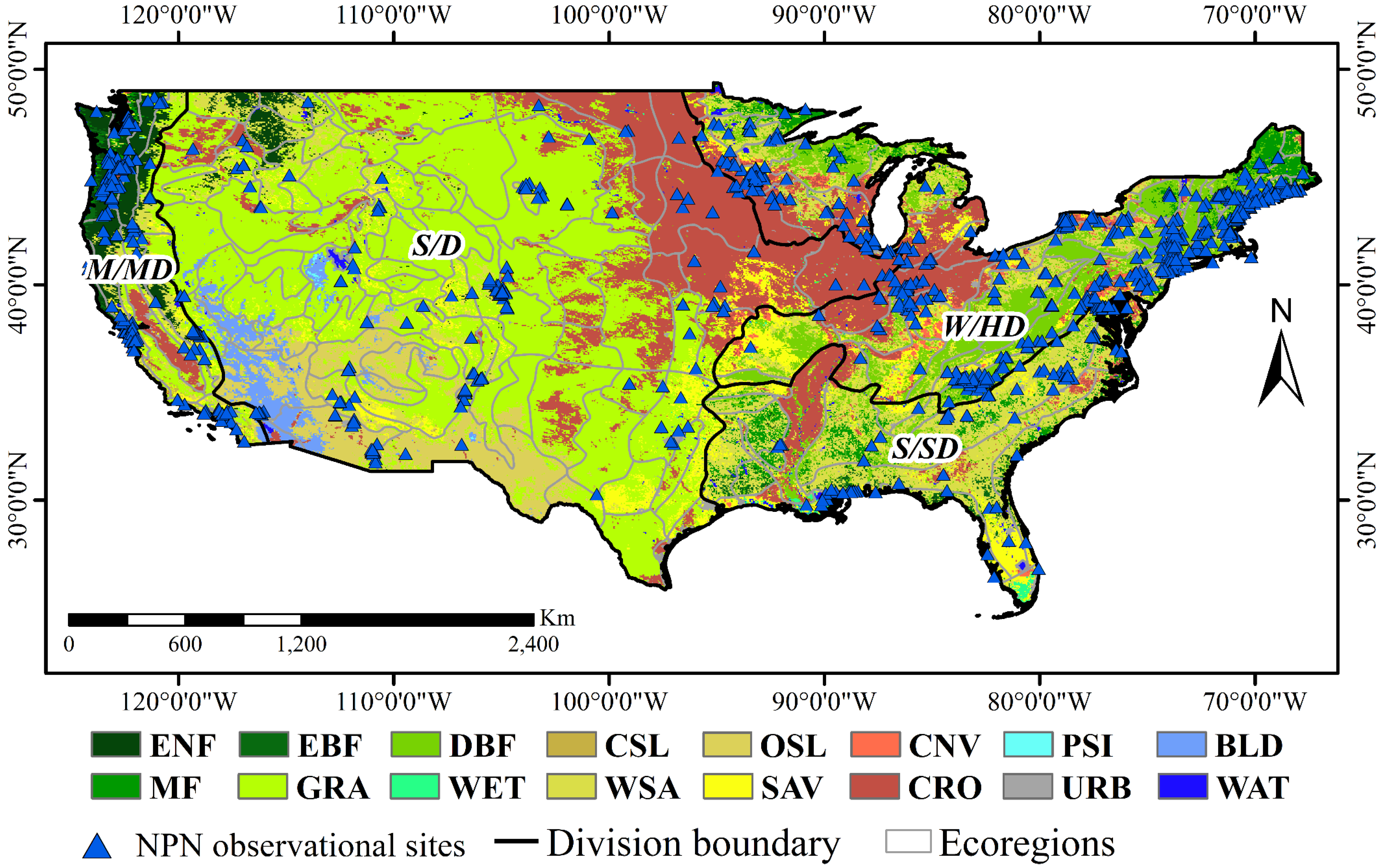
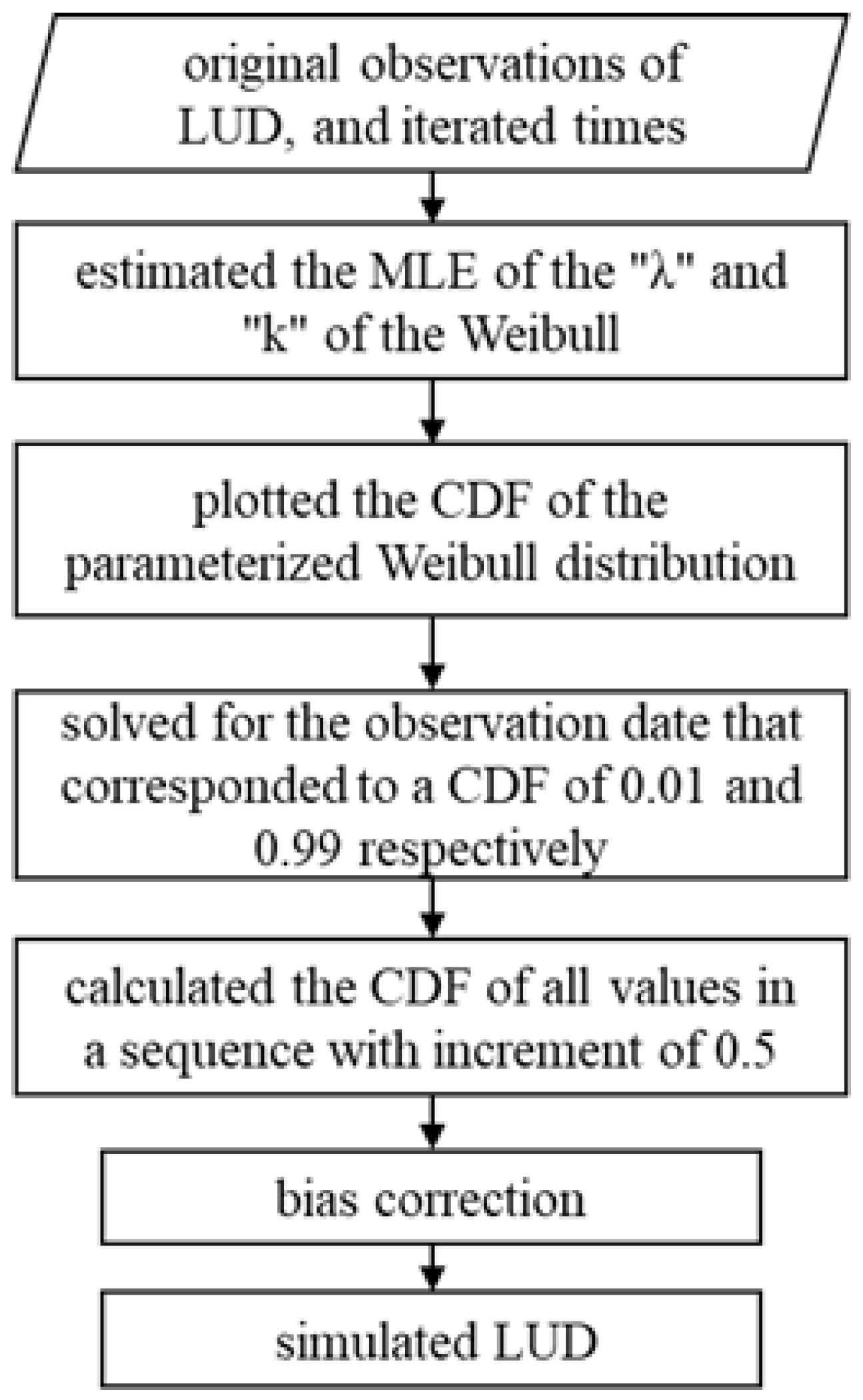
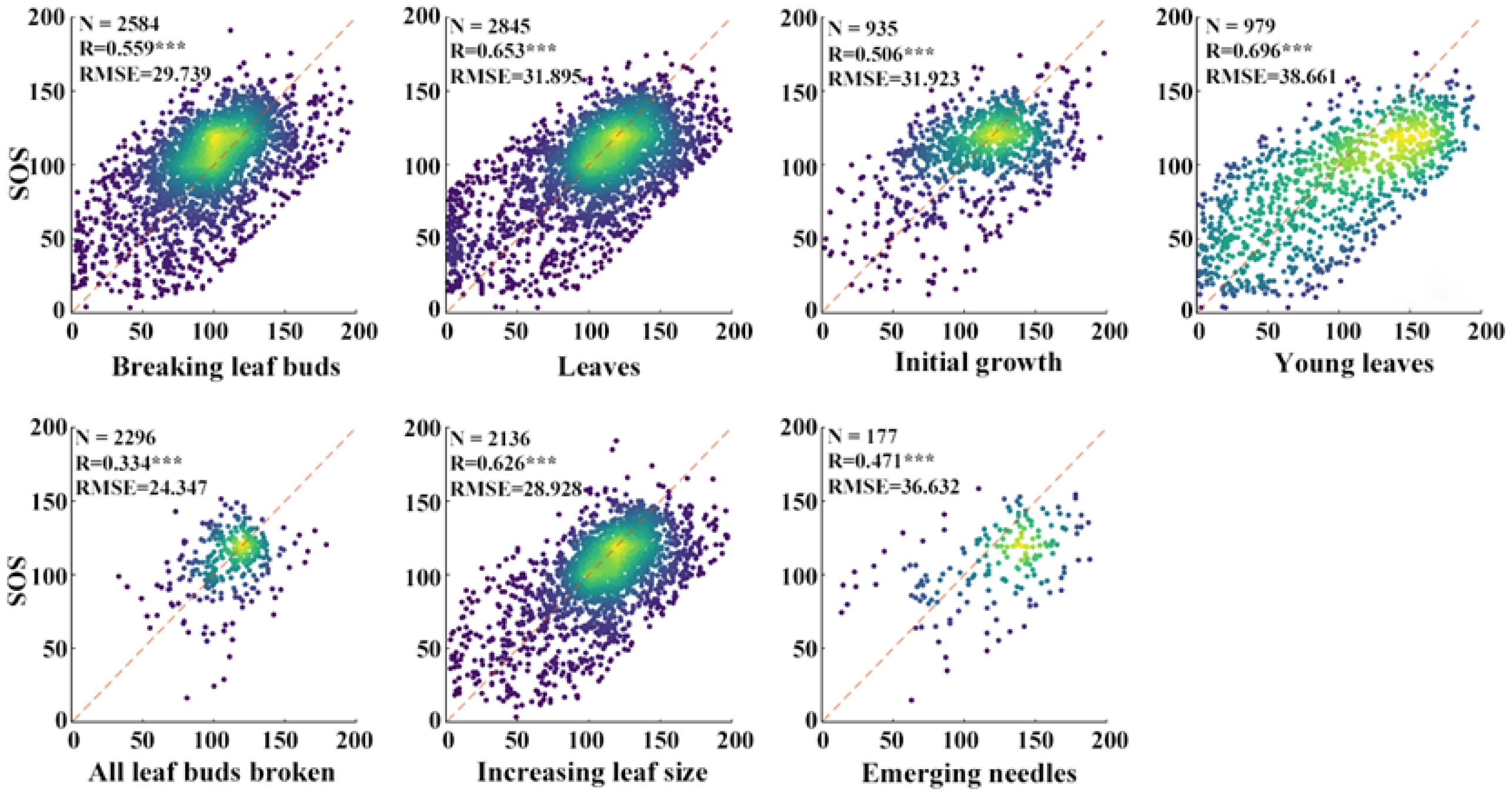
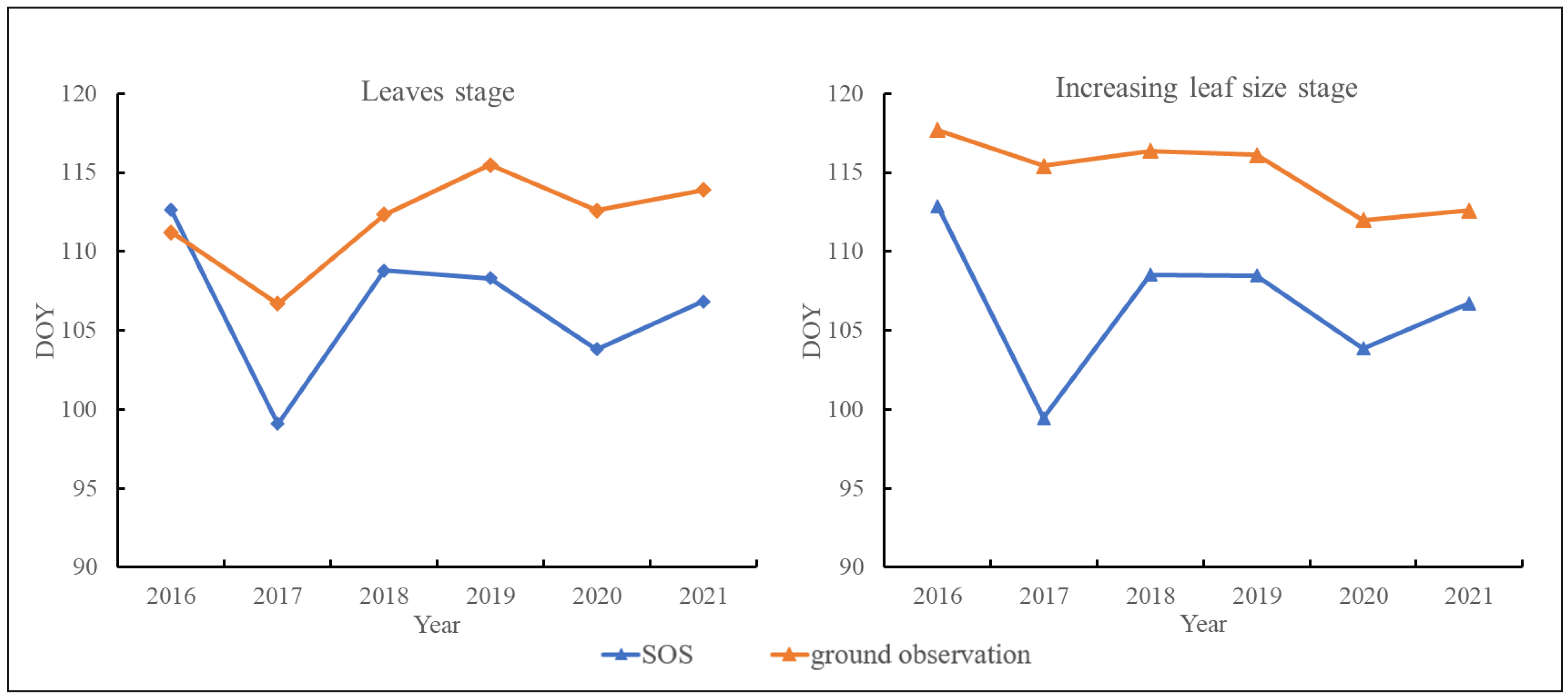
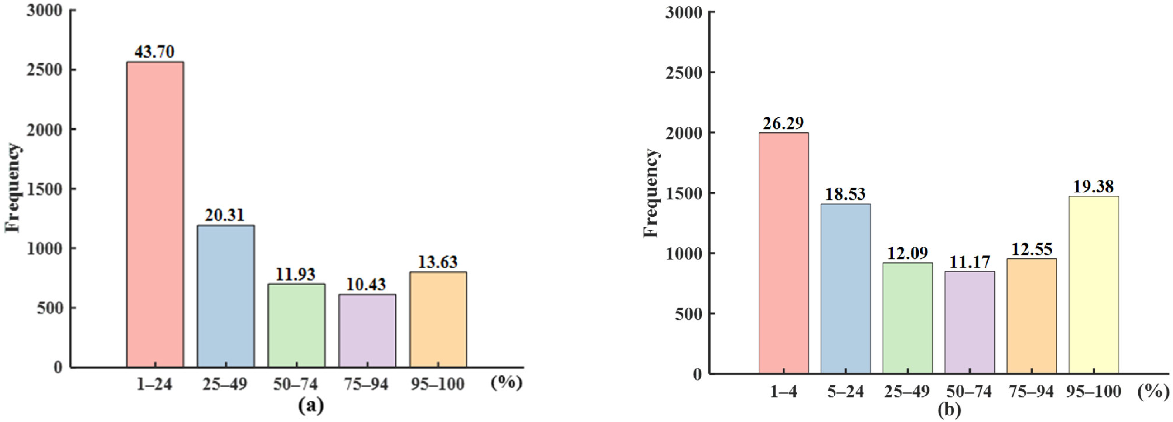

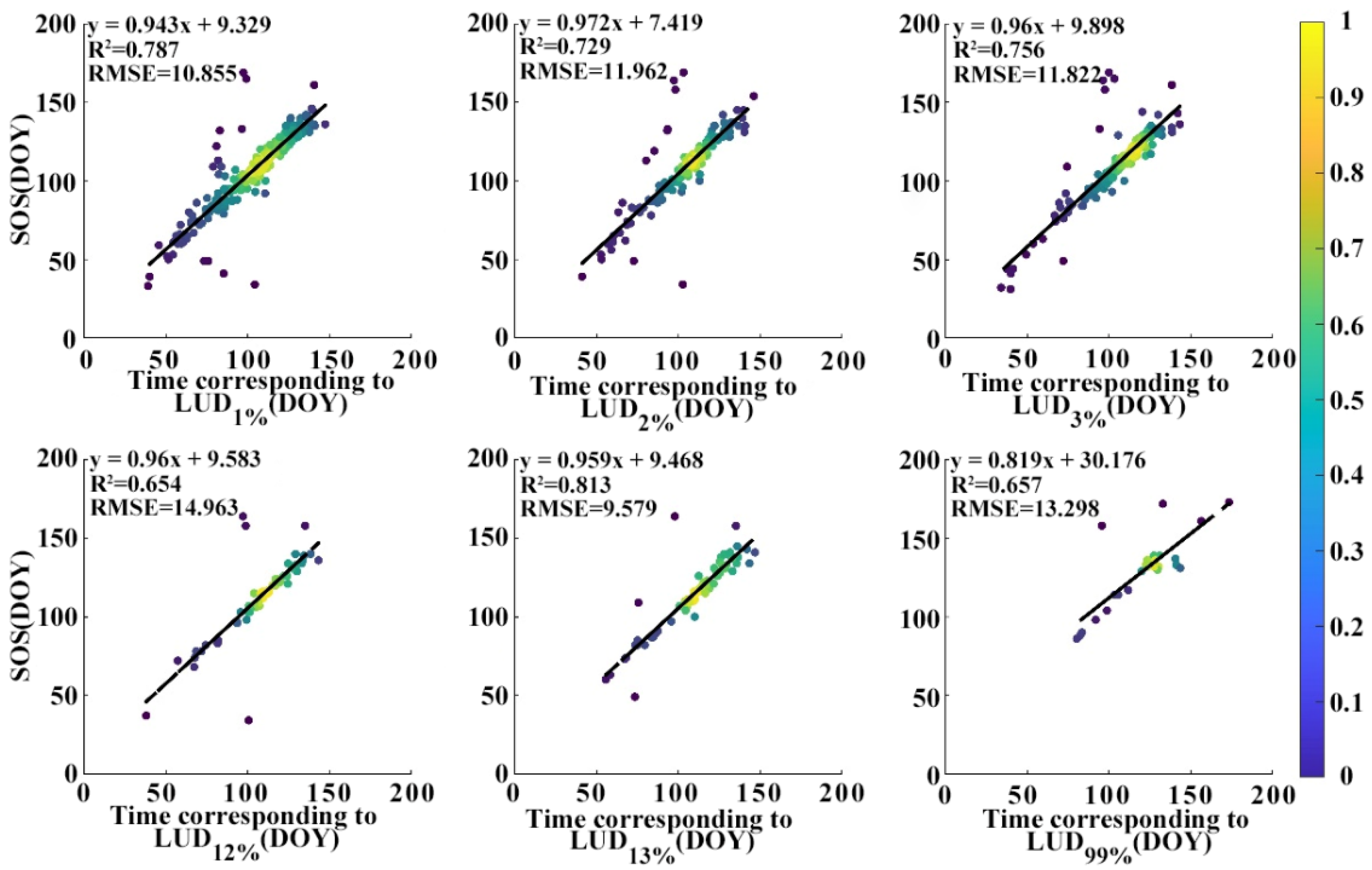
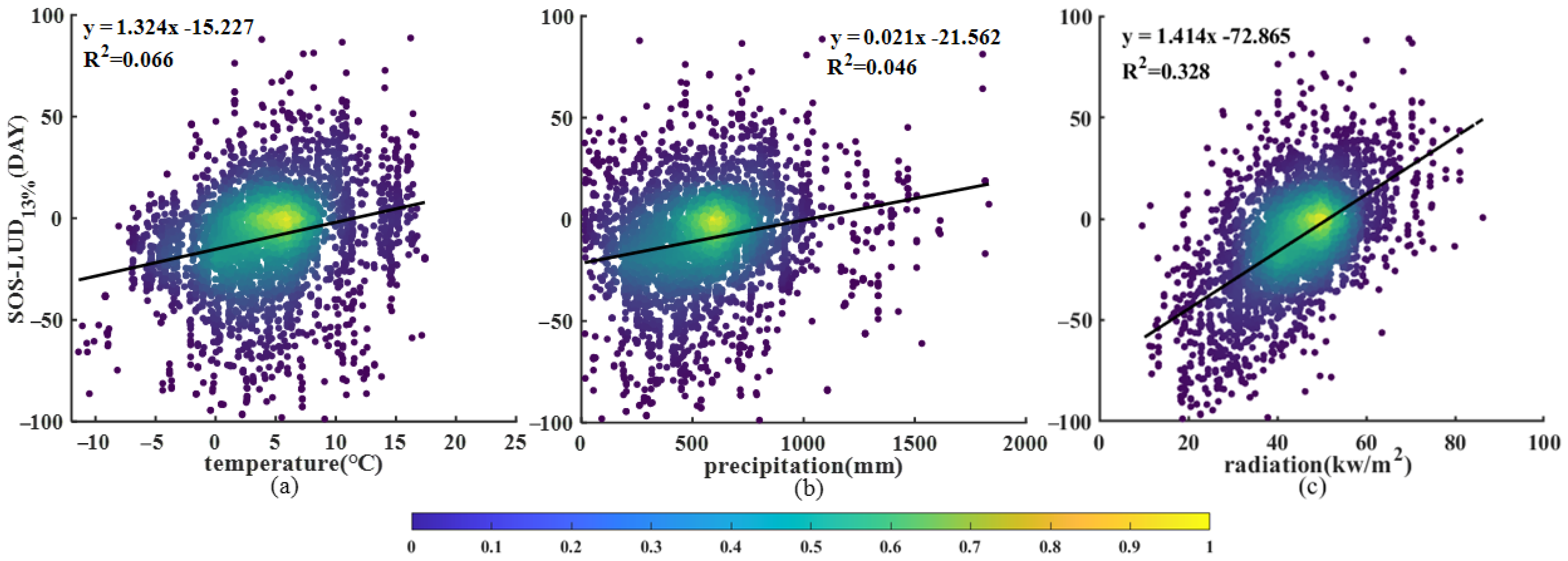
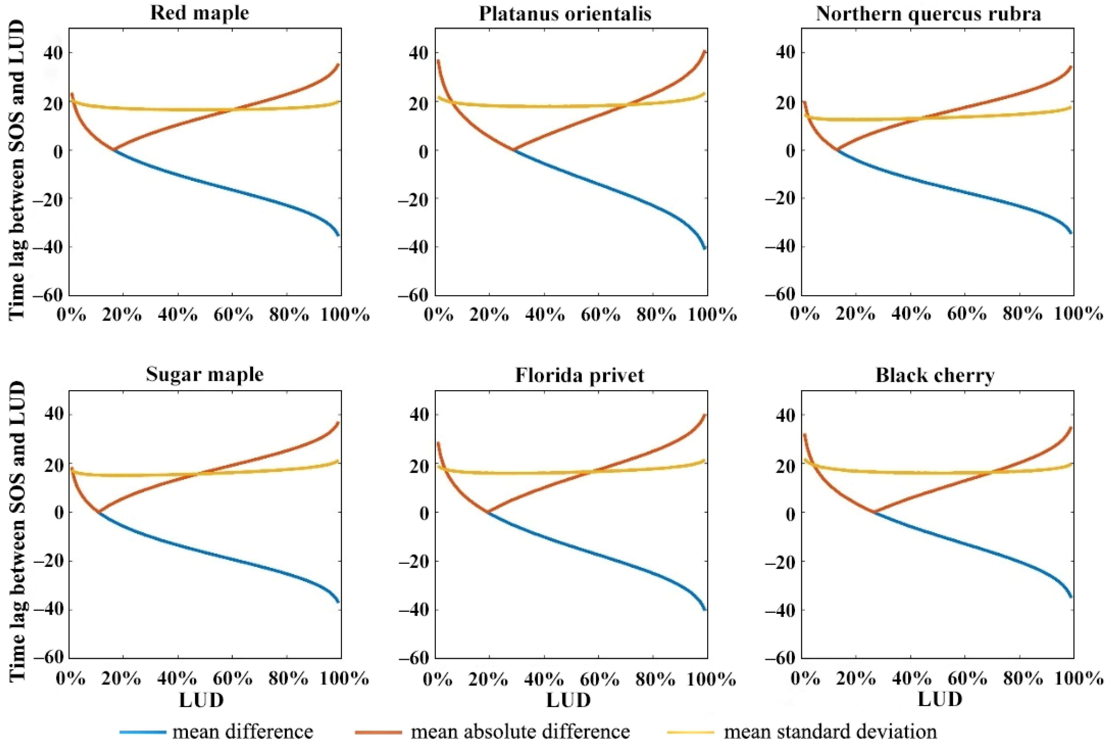
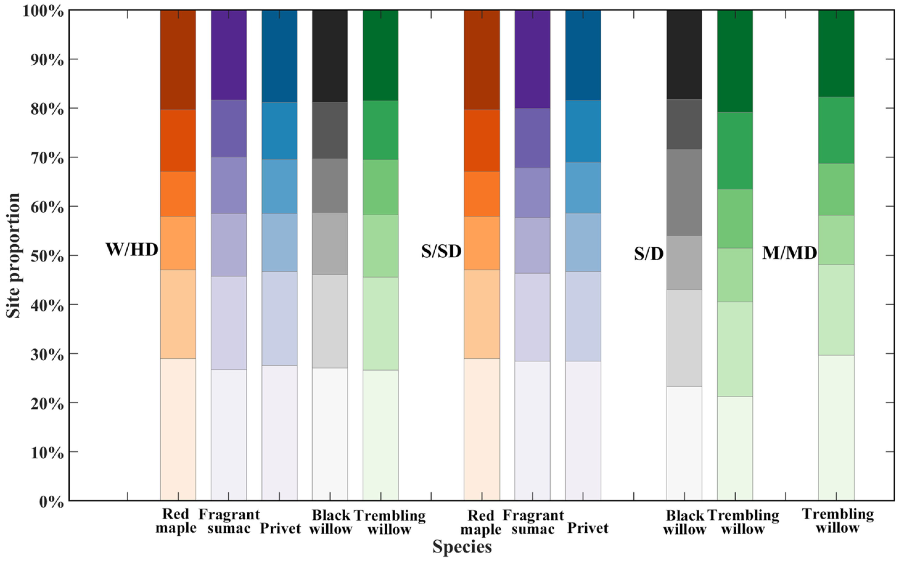
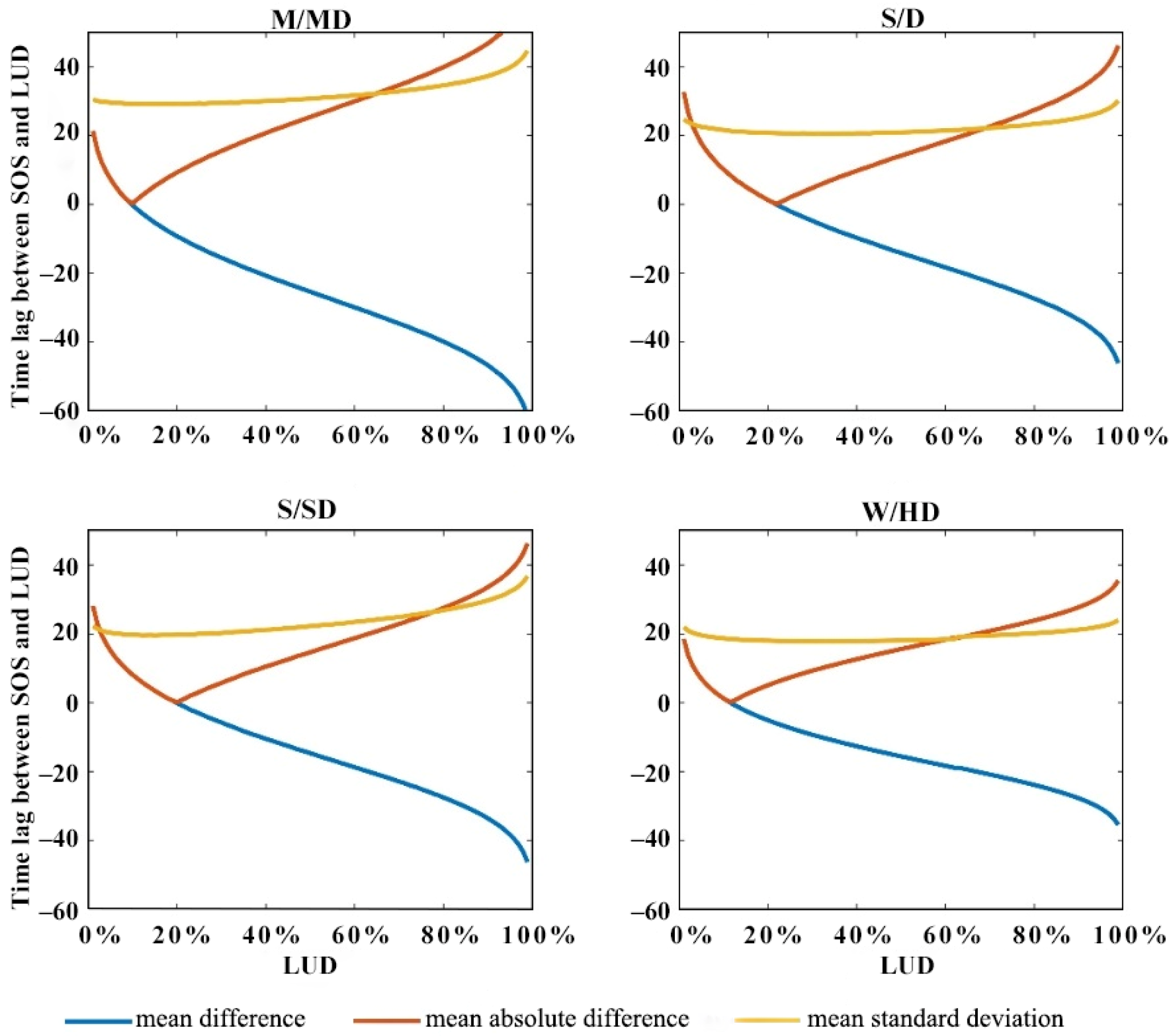
Disclaimer/Publisher’s Note: The statements, opinions and data contained in all publications are solely those of the individual author(s) and contributor(s) and not of MDPI and/or the editor(s). MDPI and/or the editor(s) disclaim responsibility for any injury to people or property resulting from any ideas, methods, instructions or products referred to in the content. |
© 2024 by the authors. Licensee MDPI, Basel, Switzerland. This article is an open access article distributed under the terms and conditions of the Creative Commons Attribution (CC BY) license (https://creativecommons.org/licenses/by/4.0/).