Abstract
In remote sensing image processing, the segmentation of clouds and their shadows is a fundamental and vital task. For cloud images, traditional deep learning methods often have weak generalization capabilities and are prone to interference from ground objects and noise, which not only results in poor boundary segmentation but also causes false and missed detections of small targets. To address these issues, we proposed a multi-branch attention fusion network (MAFNet). In the encoder section, the dual branches of ResNet50 and the Swin transformer extract features together. A multi-branch attention fusion module (MAFM) uses positional encoding to add position information. Additionally, multi-branch aggregation attention (MAA) in the MAFM fully fuses the same level of deep features extracted by ResNet50 and the Swin transformer, which enhances the boundary segmentation ability and small target detection capability. To address the challenge of detecting small cloud and shadow targets, an information deep aggregation module (IDAM) was introduced to perform multi-scale deep feature aggregation, which supplements high semantic information, improving small target detection. For the problem of rough segmentation boundaries, a recovery guided module (RGM) was designed in the decoder section, which enables the model to effectively allocate attention to complex boundary information, enhancing the network’s focus on boundary information. Experimental results on the Cloud and Cloud Shadow dataset, HRC-WHU dataset, and SPARCS dataset indicate that MAFNet surpasses existing advanced semantic segmentation techniques.
1. Introduction
In remote sensing image processing, detecting clouds and their shadows is a crucial challenge. Clouds serve as significant meteorological indicators and their variations can reflect climate changes. Accurate cloud detection improves the accuracy of weather forecasts, which helps prevent disaster weather. Nevertheless, clouds and their shadows often obscure the actual ground situation in remote sensing images, resulting in incomplete image information. By accurately segmenting clouds and cloud shadows, these image datasets can be interpreted and utilized more accurately.
The traditional threshold method [1,2,3] is suitable for cloud detection tasks in most scenes. It can be flexibly adjusted according to different scenes and needs, which makes it easy to optimize. However, it is easily affected by factors such as lighting and brightness, making it less effective in complex situations. For example, Kegelmeyer used simple pixel-based thresholds for cloud detection [4]. Despite its simplicity and feasibility, this method can result in many omissions and misjudgments in cloud detection. Zhu et al. [1] introduced the object-oriented function of mask (Fmask) cloud detection technique for Landsat remote sensing images. Although experimental results show that the Fmask method enhances cloud detection accuracy, it still falls short in effectively detecting thin clouds.
In comparison to the conventional threshold approach, deep learning approaches have good universality and better prediction performance, making them prevalent in cloud detection research. Deep learning methods improve prediction performance by training datasets and achieve end-to-end training [5,6]. The original convolutional neural network (CNN) in deep learning is a common basic image classification method. Some CNN-based methods [7,8,9] have excellent performance in image classification, laying the groundwork for pixel-level classification tasks, namely semantic segmentation. For semantic segmentation of images, Long et al. [10] introduced a fully convolutional network (FCN). This method replaces fully connected layers with convolutional layers and has proven to be effective at such tasks. Ronneberger et al. [11] developed a U-shaped network structure (UNet), which introduced skip connections between encoding and decoding layers to merge shallow and deep features. Numerous experiments have proven that UNet achieves good results in processing small samples. Zhuo Zhao et al. [12] proposed a pyramid scene parsing network (PSPNet), utilizing a pyramid pooling module (PPM) to integrate multi-scale features, thereby obtaining more global information. Yu et al. [13] introduced a bilateral segmentation network (BiseNet). BiseNet uses a bilateral segmentation architecture where different branches extract different types of information, enabling the effective combination of detailed and semantic information. HRViT [14] and HRNet [15] extract multi-scale information from the same feature map, improving robustness and generalization capability. Chen et al. [16] proposed DeepLab, which utilizes atrous convolution to expand the receptive field and conditional random fields (CRF) to enhance the model’s ability to acquire detailed information.
However, characteristics of cloud images(small scale, high similarity) bring semantic segmentation new challenges. CNN-based models often downsample features to decrease calculations, but this can result in the loss of small-scale features [17,18]. Foreground and background probably possess similar materials, features, and sizes, making them easy to be mistakenly identified. Thus, global features are needed to help segment cloud images.
Transformers’ success has opened new research paths for global modelling. Transformers are commonly used sequence prediction models in natural language processing. Carion et al. [19] introduced DETR, which utilizes the encoder–decoder structure of the transformer to model interactions within a sequence. The introduction of vision transformer (ViT) [20] and Swin transformer [21] into computer vision has significantly impacted the field. ViT was specifically designed for image classification. A pyramid vision transformer (PVT) proposed by Wang et al. [22] introduced a pyramid architecture within a transformer. Wu et al. [23] developed a convolutional vision transformer (CVT), taking the lead in combining convolution with self-attention. This approach extracts important details by using convolution while focusing on global information, which enhances the transformer’s applicability in visual tasks. The Swin transformer introduced a hierarchical design and a sliding window method, which is more efficient for processing images and more flexible for handling multi-scale tasks.
Some CNN-based networks are limited to extracting features from the receptive field through filters, establishing dependencies only within local areas. Transformer models can consider the entire input sequence at once, thereby obtaining global contextual information, but they are less adept at capturing detailed information. In the field of cloud and cloud shadow semantic segmentation, Lu et al. [24] proposed a dual-branch network (DBNet) that leverages both CNN and a transformer to achieve end-to-end cloud and cloud shadow segmentation. Gu et al. [25] proposed a multi-path multi-scale attention network (MMANet), combining CNN and a transformer to balance spatial and detailed information, thereby helping the model extract features more effectively. Inspired by the success of Lu et al. [24] and Gu et al. [25] in leveraging CNN and a transformer, our paper proposed a multi-branch attention fusion network (MAFNet). We used a combination of ResNet50 and the Swin transformer as the backbone, taking advantage of extracting local depth information and modeling long-range dependencies [26]. We introduced a multi-branch attention fusion module (MAFM), and the MAFM can add location information. The multi-branch aggregation attention (MAA) in the MAFM facilitates interaction between deep features at the same level, which improves the segmentation of boundaries and the detection of small objects. We used an information deep aggregation module (IDAM) to aggregate multi-scale features, enriching high-level semantic information and enhancing the thin cloud and point cloud detection. A recovery guided module (RGM) was used in the decoding section to enhance the network’s attention to complex boundary features, improving the restoration of cloud and cloud shadow boundaries. However, MAFNet combines ResNet50 and the Swin transformer, which require a large number of parameters and have high computational complexity, resulting in a high demand for GPUs. Therefore, MAFNet is not suitable for processing large-scale remote sensing images. Our main contributions are as follows:
- We designed a multi-branch attention fusion module (MAFM), increasing the positional information of feature maps. The multi-branch aggregation attention (MAA) in the MAFM fully fuses local and global information, enhancing the boundary segmentation capability and the detection capability of small targets.
- To enhance the detection capability of small targets, we designed an information deep aggregation module (IDAM), which performs multi-scale deep feature extraction, thereby increasing the network’s sensitivity to small targets.
- In the decoder, we introduced a recovery guided module (RGM), which adjusts the attention distribution of feature maps in the spatial dimension, enhancing the network’s focus on boundary information and enabling finer boundary segmentation.
2. Methodology
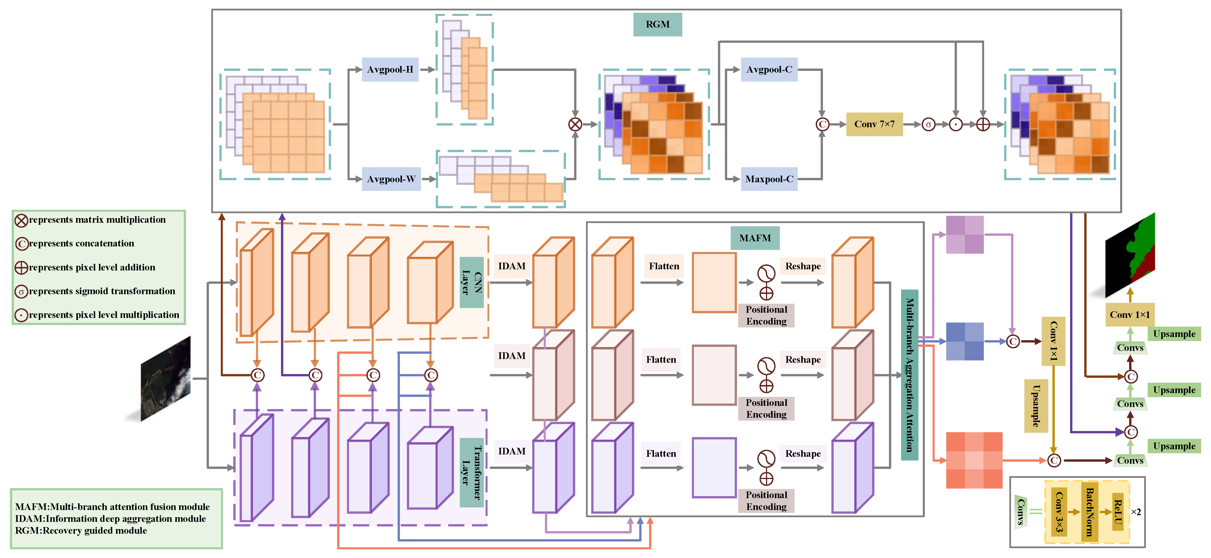
Several structures that combine CNN and a transformer have been effectively applied to remote sensing image processing [24,25,27,28] in the past years. The CNN is adept at extracting local information, while the transformer excels at extracting global information. It can better handle the segmentation of clouds and cloud shadows in complex backgrounds to combine the advantages of both. Therefore, this paper proposed a dual-branch architecture combining ResNet50 and the Swin transformer, as shown in Figure 1. This architecture yields good results in detecting small targets and segmenting boundaries. In the encoder stage, for an input image , the feature map produced by the ith layer of ResNet50 is denoted as , the feature map produced by the ith layer of the Swin transformer is denoted as , and the feature map produced by the ith fusion is denoted as . It should be noted that and the channel sizes of the feature maps produced by the ith layer of ResNet50 and the ith fusion are the same. A multi-branch attention fusion module (MAFM) adds location information to deep feature maps at the same level and utilizes multi-branch aggregation attention (MAA) to sufficiently aggregate deep features maps, enhancing the precision of cloud and cloud shadow boundary segmentation and small target recognition. An information deep aggregation module (IDAM) effectively addresses semantic gaps and small target localization errors through multi-scale feature extraction. Based on the UNet decoder, a recovery guided module (RGM) adaptively extracts spatial information from shallow feature maps obtained during the fusion section, which guides our model’s focus on boundary regions, resulting in more precise boundary segmentation.
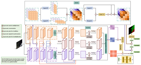
Figure 1.
Multi-branch attention fusion network structure.
2.1. Backbone
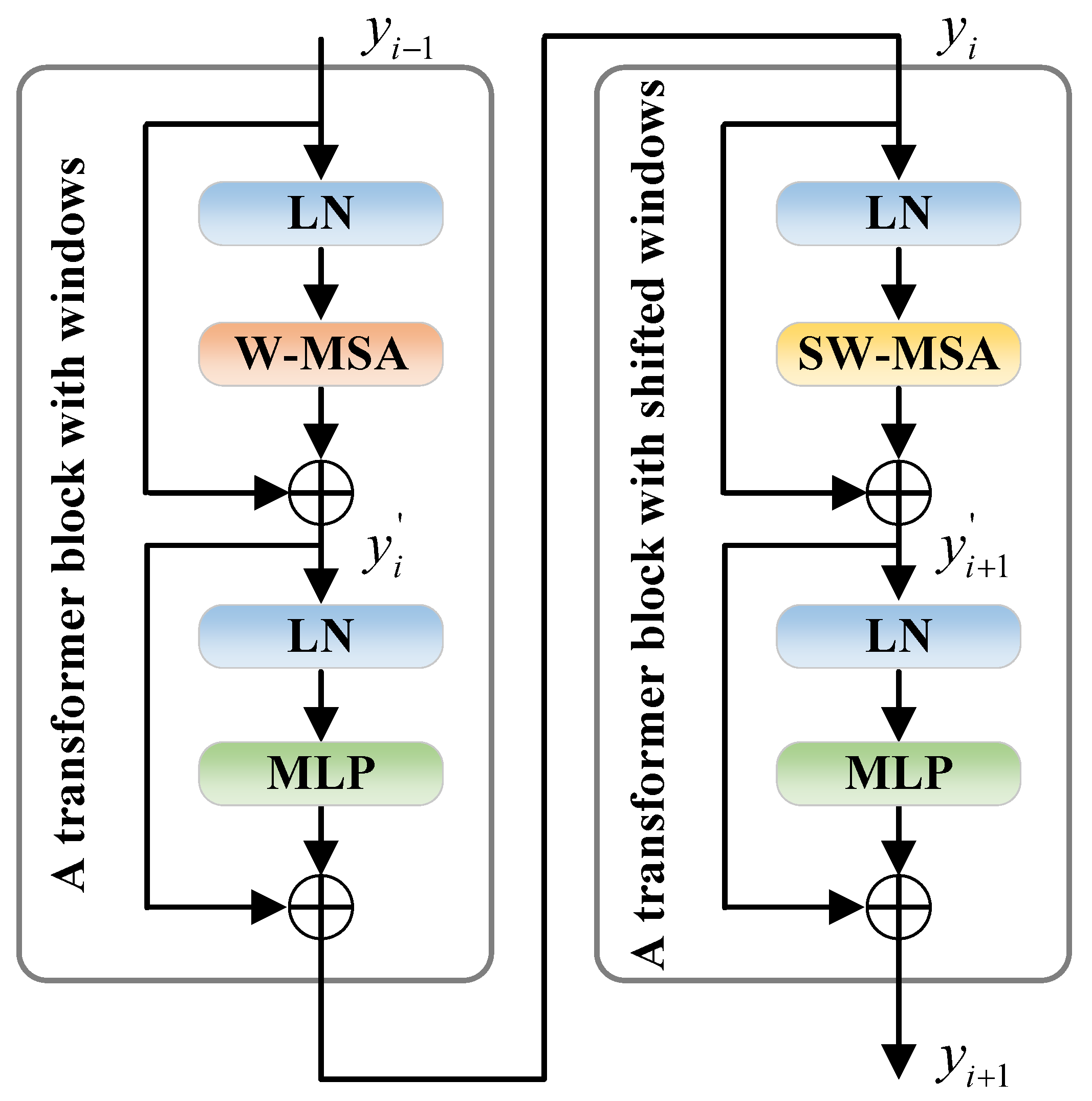
It is well known that convolutional networks possess good properties such as shift, scale, and distortion invariance, while transformers possess good properties such as dynamic attention, global receptive fields and superior generalization abilities [29,30,31]. When it comes to feature extraction, transformers can complement the CNN, enhancing the capability of extracting information and allowing for more effective extraction of high-level features. Therefore, we used ResNet50 and the Swin transformer as the backbone for feature extraction. Since ResNet50 is very common, we will not elaborate further on its structure. Next, we will focus on the Swin transformer architecture. In standard transformer blocks, multi-head self-attention (MSA) computes global attention between each patch, which results in a high computational load. Therefore, the standard transformer is not suited for high-resolution tasks such as cloud and cloud shadow semantic segmentation. To mitigate huge calculations, the Swin transformer introduces window multi-head self-attention (W-MSA) and shifted window multi-head self-attention (SW-MSA) to replace MSA. In Swin transformer blocks, a feature map is segmented into several windows, each of which contains multiple patches. W-MSA and SW-MSA compute attention in the window while ignoring patches outside the window, significantly reducing computational complexity. Unlike W-MSA, which only confines attention within the window, SW-MSA still uses window offset to achieve communication between windows. Figure 2 illustrates the two types of Swin transformer blocks: a transformer block with windows and a transformer block with shifted windows. The two blocks always alternate in continuous Swin transformer blocks. The formulas used in the Swin transformer blocks are as follows:
where represents the layer normalization operation, represents the operation performed by the multi-layer perceptron, and , , and represent the outputs of the ()th, ith, and ()th Swin transformer blocks, respectively. Moreover, and represent the intermediate values of the ith and th Swin transformer blocks, respectively.
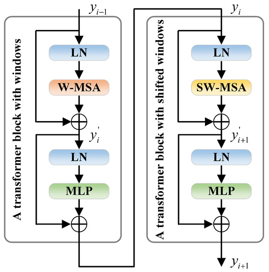
Figure 2.
Two consecutive Swin transformer blocks.
2.2. Multi-Branch Attention Fusion Module
Before fully integrating local and global features, we need to apply positional encoding to the three input feature maps. In transformer architectures, positional encoding is commonly used to handle the flattened feature maps, providing each pixel with positional information. To avoid tedious repetition, we will only focus on the operations for , , and . First, it is necessary to perform the flatten operation to achieve dimensionality reduction. The specific size changes are as follows:
where we use ’×’ to denote size changes of feature maps. It should be noted that positional encoding does not alter the dimensions of a feature map. The encoded , , and perform the reshape operation to restore to the sizes of their corresponding original feature maps. The specific size changes are as follows:
The obtained , , and will be input into a multi-branch aggregation attention (MAA) to fully integrate local and global features.
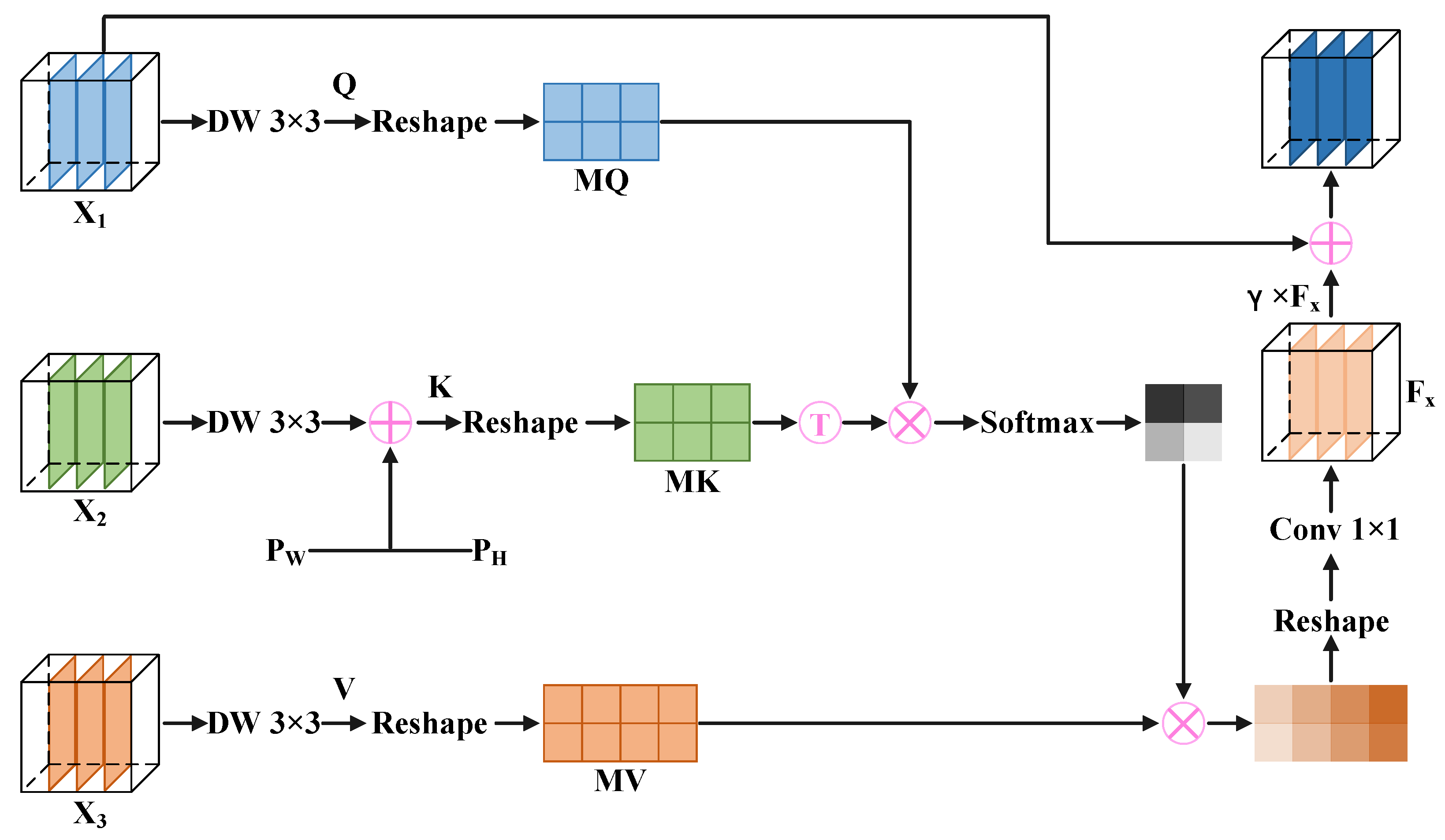
Multi-branch aggregation attention: To make the cloud and cloud shadow segmentation boundaries fine and enhance the capability of small target detection, inspired by the self-attention mechanism in the VIT [20], we designed a multi-branch aggregation attention (MAA) in the multi-branch attention fusion module (MBAF). Figure 3 displays the structure of the MAA. We apply a depthwise separable convolution with a kernel size to , , and , generating query , key , and value . Compared to a conventional 2D convolution with a kernel size, the depthwise separable convolution with a kernel size significantly reduces computation when generating Q, K, and V. Notably, the common attention calculation only requires a single input feature map to yielding Q, K and V, while MAA requires three different input feature maps. After convolution, we embed two updatable vectors into K. One denoted as represents horizontal spatial attention, while the other denoted as represents vertical spatial attention. The formulas are as follows:
where represents a depthwise separable convolution operation with a kernel size, , and . Notably, and can update gradients during backpropagation, thereby optimizing pixels in the W and H dimensions, which achieves a calibration effect on K. Next, we perform rearrange operations on Q, K, and V separately to divide them into multiple heads, obtaining , , and . Then, we use , , and to obtain a weighted feature map. The formulas are as follows:
where represents the arrange operation, , , , and represents the number of heads in the multi-head attention. Compared to the single-head attention mechanism, the multi-head attention mechanism significantly improves the model’s expression and feature extraction ability by computing multiple attention heads in parallel. ⊗ represents matrix multiplication, represents the transpose operation, is a common normalization operation, and represents the weighted feature map. Next, we apply the arrange operation and the convolution with a kernel size to to ensure its size matches that of . We denote the resulting feature map as . There is a learnable parameter is set to calibrate . Finally, we introduce a skip connection to add the calibrated to , obtaining an output feature map which contains high-level semantic information. Overall, MAFM improves the localization ability of small targets by adding positional information, while the novel multi-head attention mechanism in the MAA enhances attention to complex segmentation boundaries, making segmentation boundaries finer. The formulas are as follows:
where represents the convolution with a kernel size, , and . Additionally, represents the output of the MMA.

Figure 3.
Multi-branch aggregation attention.
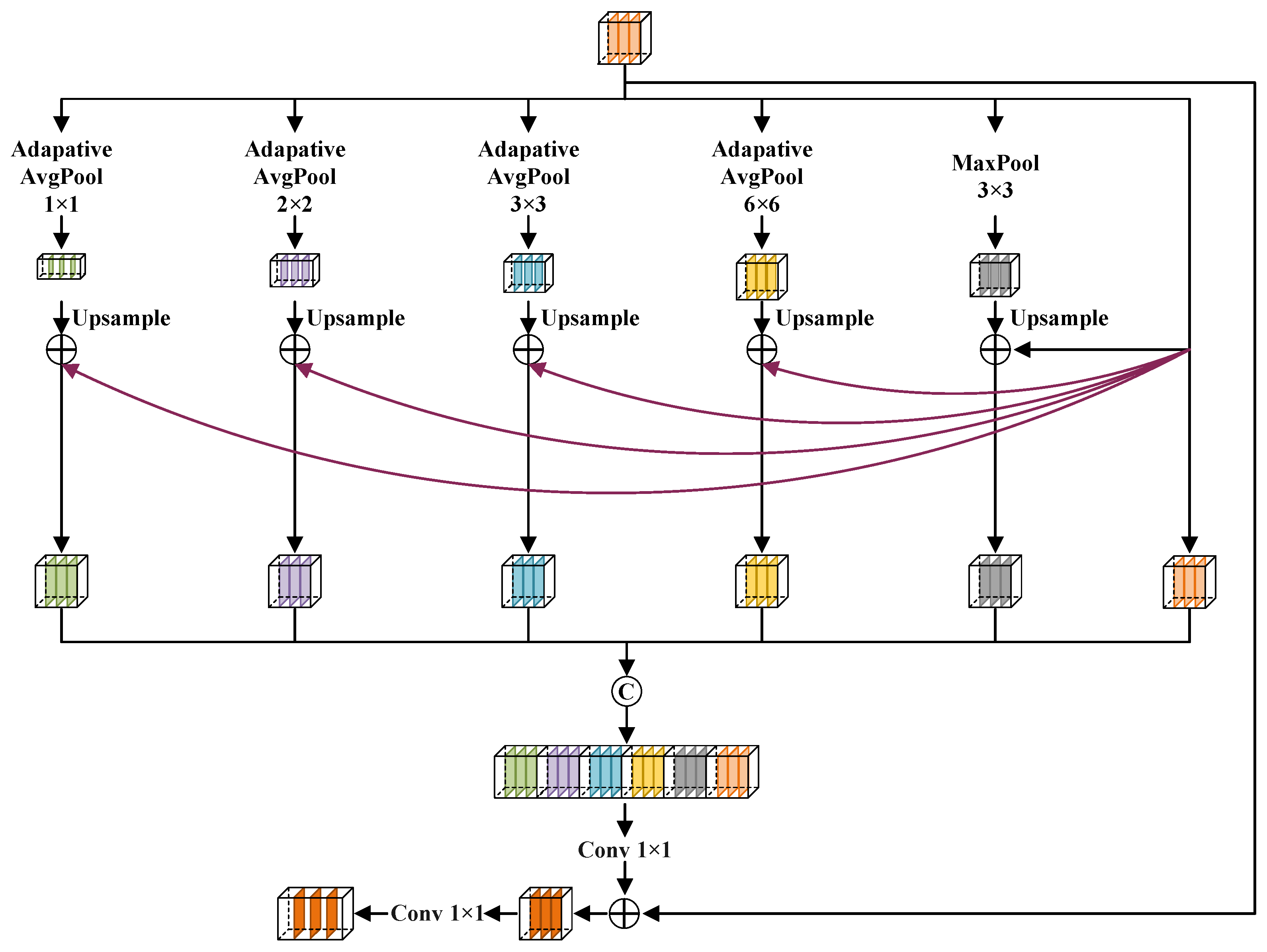
2.3. Information Deep Aggregation Module
Effectively extracting small target features for the semantic segmentation of remote sensing images faces significant challenges. For example, DeepLab [16] uses atrous convolutions to increase the receptive field, fully extracting high semantic information. However, atrous convolutions can make the model insensitive to small-scale targets, leading to missed or false detections. To enhance the capability of our model to recognize small targets, we designed an information deep aggregation module (IDAM). Figure 4 shows the structure of the IDAM.
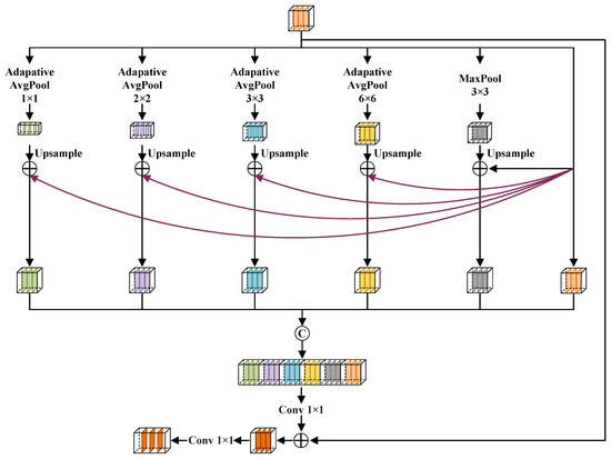
Figure 4.
Information deep aggregation module.
First, the IDAM conducts multi-scale pooling operations on the input feature map to deeply extract information. Next, each pooled feature map, after being upsampled to match the size of the original feature map, has the input feature map added to it through pixel-wise addition. Subsequently, the input feature map and resulting feature maps and are concatenated, achieving deep aggregation of multi-scale features. Then, the feature map obtained through concatenation undergoes the convolution operation with a kernel size to adjust the quantity of channels to that of the input, followed by pixel-level addition with the input. The addition operation not only avoid gradient disappearance and explosion but also uses low-level features to help the high-level feature segmentation become more refined. Eventually, conducting a convolution with a kernel size on the result from the addition to obtain the desired quantity of channels. Overall, in the IDAM, multi-scale feature extraction and deep integration of contextual information can help capture the details and semantic information of small targets, effectively reducing missed and false detections of small targets. The formulas are as follows:
where denotes the input of the IDAM, denotes the multi-scale pooling operation, denotes the upsampling operation, denotes the convolution operation with a kernel size, denotes the concatenation operation, and denotes the output feature map of the IDAM.
2.4. Recovery Guided Module
Firstly, semantic dilution inevitably occurs in the decoding stage of semantic segmentation networks based on encoders and decoders [32]. Secondly, clouds and cloud shadows have textures similar to the background, irregular shapes, and indistinct target features. Their colour depth is easily affected by factors like weather, making cloud and cloud shadow semantic segmentation highly susceptible to background noise. The above two issues can result in poor boundary segmentation. Inspired by the spatial attention module (SAM) [33], based on the UNet decoder, we introduce a recovery guided module (RGM) to enhance the capability of the segmentation boundary restoration. The RGM is shown at the top of Figure 1.
First, we perform average pooling operations on the input in the H and W dimensions separately and then use matrix multiplication to reconstruct the input feature map for the first time. Next, by parallelly performing max pooling and average pooling in the channel dimension, global features are deeply extracted from the reconstruct feature map. After that, we concatenate the two pooled feature maps, apply convolution, and then use a sigmoid transformation to acquire the attention weights of the first reconstructed feature map. Subsequently, we multiply these weights pixel by pixel with the first reconstructed feature map, enabling a second reconstruction of the feature map. Overall, RGM uses multi-dimensional pooling to achieve secondary reconstruction on inputs acquired from the fusion section, enhancing the network’s focus on boundary features, which improves the boundary segmentation capability. The formulas are as follows:
where represents the input, , , -, and - represent the average pooling operation in the height dimension, the average pooling operation in the width dimension, the max pooling operation in the channel dimension, and the average pooling operation in the width dimension, respectively. denotes the first reconstructed feature map, denotes the convolution operation with a kernel size, denotes the sigmoid transformation, ⊙ denotes the pixel-wise multiplication operation, denotes the second reconstructed feature map, and represents the output feature map.
3. Experiments
3.1. Datasets
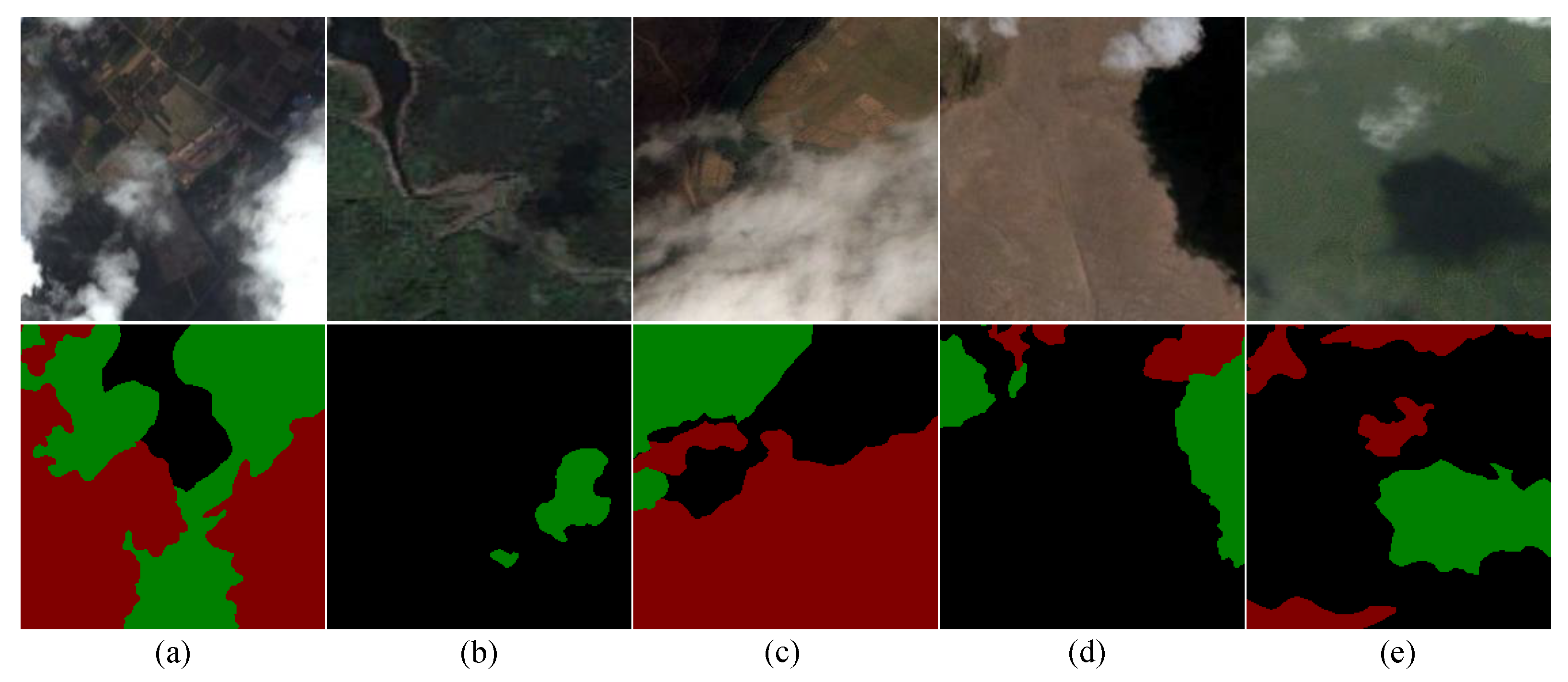
3.1.1. Cloud and Cloud Shadow Dataset
This dataset originates from data organized by Landsat-8 and Sentinel-2. Landsat-8 was developed collaboratively by the NASA and USGS. It is equipped with the operational land imager (OLI) and the thermal infrared sensor (TIRS) instruments. Both of them can obtain images with a spatial resolution of 30 m and achieve annual coverage of global regions. The sensors carried by Sentinel-2 can capture 13 different spectral bands. The spatial resolution of the images monitored by Sentinel-2 ranges from 10 m to 60 m, achieving systematic coverage of land surfaces, coastal waters, and the entire Mediterranean region from latitude south to latitude north. Since the original remote sensing images have a high-pixel resolution and the GPU memory capacity is limited, training models directly on the original images takes a long time. Therefore, we cropped the original images into small images of pixels, obtaining 25,314 samples. According to experimental requirements, these images were divided into 16,000 training samples, 4000 test samples, and 5314 validation samples. The dataset includes semantic annotations for clouds, cloud shadows, and the background to evaluate the model’s recognition capabilities in different environments. Additionally, the dataset covers a variety of complex terrains including plateaus, plains, hills, cities, and farmlands. Figure 5 shows several samples of the dataset.
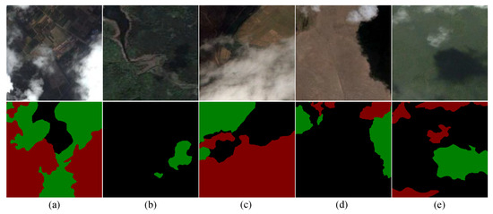
Figure 5.
Cloud and Cloud Shadow Dataset. The first row displays the cropped images which include (a) city, (b) shrubs, (c) farmland, (d) desert, and (e) forest. The second row displays corresponding labels.
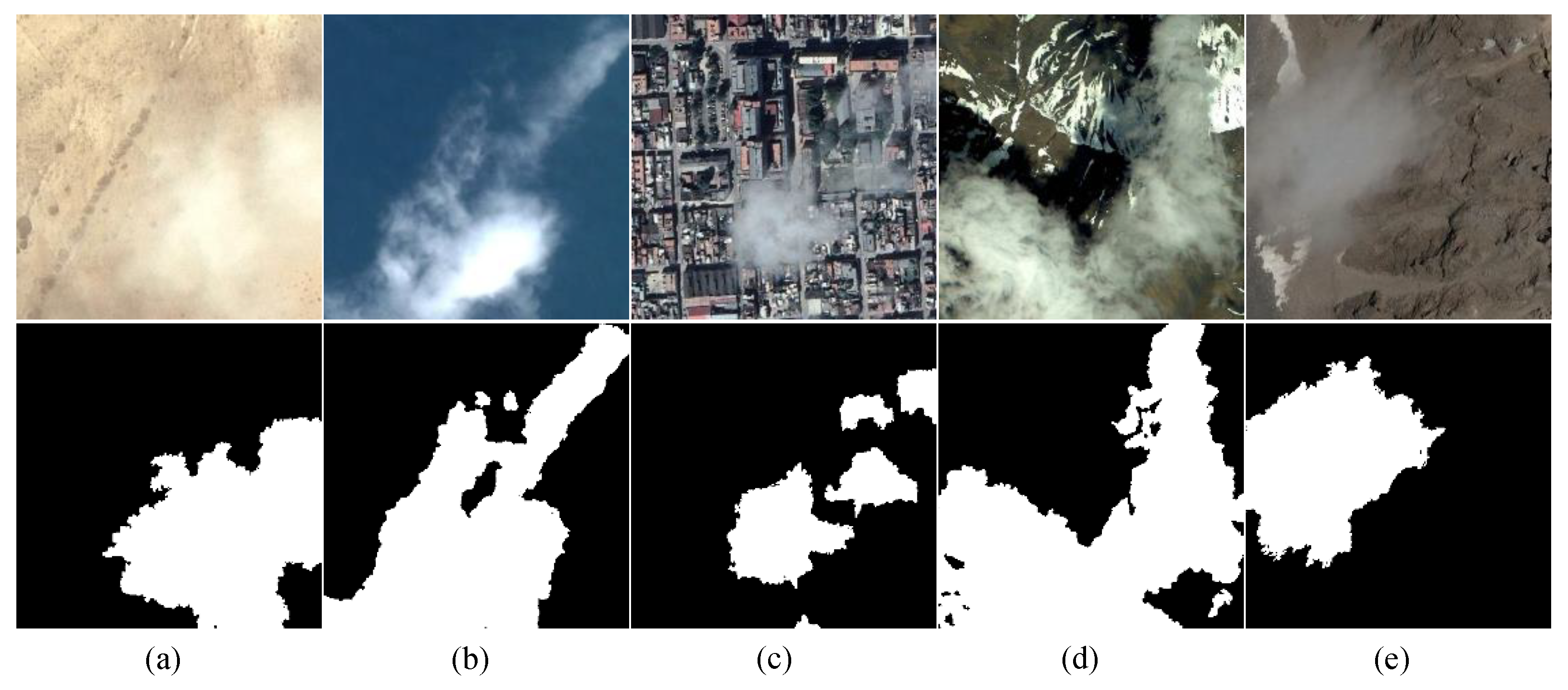
3.1.2. HRC-WHU Dataset
To evaluate the generalization capability of the model, we use the high-resolution cloud cover validation dataset created by researchers Li et al. from Wuhan University (HRC-WHU) [34]. This dataset consists of 150 images, each with three RGB channels. These images have a pixel resolution of and their spatial resolution varies from 0.5 to 15 m. We cropped these images into small images of pixels for training. To prevent model overfitting, we also performed data augmentation by flipping images, rotating images, and adding noise to the images. The dataset includes complex scenes such as snow, water, deserts, plants, and cities. Several samples of the dataset are displayed in Figure 6.

Figure 6.
HRC-WHU dataset. The first row displays the cropped images which include (a) desert, (b) ocean, (c) city, (d) ridge, and (e) snow. The second row displays corresponding labels.
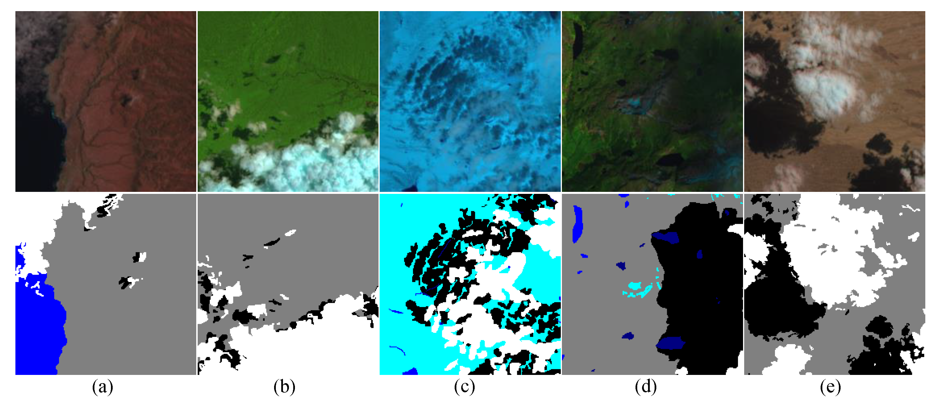
3.1.3. SPARCS Dataset
The spatial procedures for automated removal of cloud and shadow (SPARCS) [35] was used to further evaluate the generalization capability of our model. The SPARCS dataset, derived from data collected by Landsat-8, includes 80 images of pixels. We cropped them into small images of pixels, resulting in 1280 samples. Flipping and rotating operations were conducted on the cropped images to enhance the diversity of samples and the generalization performance of our model. After data augmentation, the resulting images were then divided into a training set and a validation set in an 8:2 ratio. The dataset includes multiple scenes such as fields, deserts, hills, woodlands, snow, and water. Figure 7 shows several samples of the SPARCS Dataset.

Figure 7.
SPARCS Dataset. The first row displays the cropped images which include (a) mountains, (b) forest, (c) snow, (d) wetlands, and (e) desert. The second row displays corresponding labels.
3.2. Experimental Details
The experiments were based on the PyTorch platform with an RTX 3080 GPU (NVIDIA Corporation, Santa Clara, CA, USA). We utilized the Adam optimizer to iterate the experimental parameters, with the exponential decay rate for the first moment estimate set to 0.9 and for the second moment estimate set to 0.999. The learning rate strategy adopted by us is the step learning rate schedule (StepLR). The initial learning rate was set to 0.001 and the adjustment multiplier was set to 0.95. The adjustment interval, denoted by , was set to 3. The model was trained for a total of 300 iterations, with the current number of iterations denoted by . The calculation formula of the new learning rate that is denoted by is as follows:
The loss function adopted by us is the cross-entropy loss function during the training process. Due to GPU capacity limitations, the experiments were performed with a batch size of 16. We selected precision (P), recall (R), score, pixel accuracy (PA), and mean intersection over union (MIoU) among many metrics to evaluate the segmentation performance of different models. The formulas for the above metrics are as follows:
where , , and represent the number of pixels rightly identified as the foreground, wrongly identified as the foreground, and incorrectly identified as the background, respectively. k denotes the number of classes (excluding the background). , , and denote the number of pixels rightly identified as class i, the number of pixels of class i identified as class j and the number of pixels of class j identified as class i, respectively.
3.3. Network Backbone Selection
Before the ablation and comparative experiments, we selected six dual-branch structures to screen the best network backbone. Table 1 displays the comparison results. According to the results, the optimal network backbone is our Swin + ResNet50, which achieves the highest scores in both and MIoU. Next, we analysed why Swin + ResNet50 is the best in terms of network structure. Compared to the MSA in PVT and CVT, which calculates global attention on the feature maps and only focuses on global information, the W-MSA (Figure 2) in the Swin transformer calculates local attention within each window, capturing local contextual information. Furthermore, The SW-MSA (Figure 2) facilitates communication between windows through window offset, which takes into account global information, so Swin is superior to PVT and CVT. ResNet50, with more network layers than ResNet34, has deeper abstraction and analytical capabilities when processing image features, which help it extract more high-level semantic information, so ResNet50 is superior to ResNet34. Overall, from the perspective of both experimental results and network structures, our Swin + ResNet50 is the optimal backbone network.

Table 1.
Selection of different backbones (bold represents the best result).
3.4. Network Fusion Experiment
To obtain the best fusion method, we conducted comparative experiments on the encoder fusion section. The comparison results are shown in Table 2, where , + and ⊙ denote the concatenation, the pixel-wise addition and the pixel-wise multiplication, respectively. The optimal fusion method is the concatenation, which achieves the highest and MIoU scores. Compared to the concatenation, which preserves all feature maps, the pixel-wise addition and multiplication merge features through pixel-wise numerical operations, resulting in feature loss.
Table 2.
Selection of fusion methods (bold represents the best result).
Next, we conducted comparative experiments to determine whether the feature maps obtained from the fusion section should be processed by the RGM. The comparison results are displayed in Table 3, where (i) indicates the feature map from the ith fusion stage () is processed by the RGM and . The optimal method is (1) + (2), which achieves the highest and MIoU scores. This is because both and are derived from deeper layers of the network, allowing the RGM to process the two feature maps causes the model to learn noise, which inevitably results in overfitting.
Table 3.
Selection of RGM inputs (bold represents the best result).
3.5. Ablation Experiments on Cloud and Cloud Shadow Dataset
We performed ablation experiments on this dataset to better understand the structure and function of various modules. Firstly, we used the ResNet50 with the UNet decoder as a reference and gradually add modules to better understand their impact on model performance. In subsequent ablation experiments, we used MIoU for evaluation. Table 4 displays the results of ablation experiments, indicating that our proposed model has the optimal performance.
Table 4.
Ablation for different modules (bold represents the best result).
- Ablation for Swin: To enhance global modelling capabilities, we introduced a Swin transformer based on the ResNet50 architecture. Table 4 indicates that MIoU is 0.41% higher than that of the simple ResNet50, which adequately demonstrates that it can strengthen the performance of our model to extract global information utilizing the Swin transformer.
- Ablation for MAFM: To improve the boundary segmentation of clouds and their shadows, as well as the detection capability of small objects, we introduced MAFM. The MAFM enhances the positional information of feature maps. Its MMA allows deep features at the same level to guide each other, fully fusing fine and rough features. Table 4 indicates that the introduction of the MAFM improves the MIoU by 1.10%, which demonstrates the MAFM is effective in the semantic segmentation of clouds and their shadows.
- Ablation for IDAM: To further enhance the localization capability for small target clouds and cloud shadows, we introduced IDAM to extract deep features at multiple scales and supplement high semantic information, thus increasing sensitivity to small targets. Table 4 indicates that the introduction of IDAM can improve the MIoU by 0.57%.
- Ablation for RGM: Fine boundary segmentation has always been a major challenge in the segmentation of clouds and their shadows. To address this issue, we added the RGM based on the UNet decoder. The RGM can focus the model on important information in the feature map, enhancing the model’s focus on complex boundary features. As shown in Table 4, the introduction of the RGM improves the MIoU by 0.39%, which sufficiently demonstrates that the RGM effectively facilitates the refinement of segmentation boundaries.
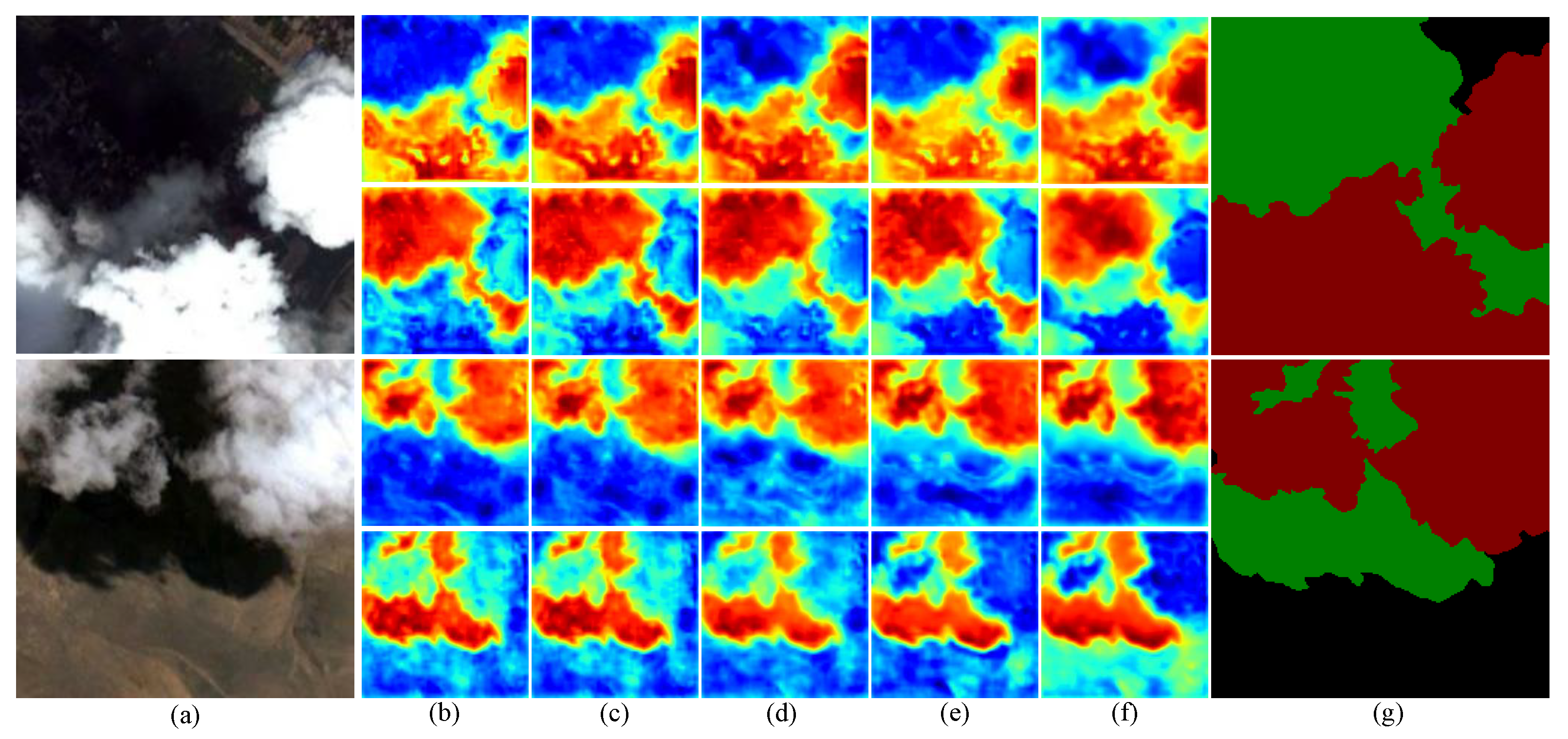
More intuitively, Figure 8 shows the ablation heatmaps for two images including clouds and their shadows. In the heatmap grid, the first and third rows show heatmaps related to clouds, while the second and fourth rows show heatmaps related to cloud shadows. In these heatmaps, red areas acquire high attention, while blue areas require no attention. Next, we will assess the performance of each module using the heatmaps and the score metric. Figure 8a displays the prediction situation of ResNet50, indicating that the pure convolutional network can effectively locate cloud shadows, but it has a high false detection rate at the edges of clouds. The segmentation results obtained using the pure convolutional network significantly differ from the corresponding label, with the corresponding in Table 4 being only 90.55%, which is the lowest value. Due to the fact that the pure convolutional network only has local perception ability and lacks global modelling ability, we introduced the Swin transformer. Compared to Figure 8b, in Figure 8c, there is a noticeable increase in the red areas of the heatmaps for clouds and cloud shadows, and the classification results are more similar to the corresponding labels. Since the self-attention mechanism in the Swin transformer adjusts the attention distribution of feature maps, it allows our model to pay attention to more critical regions and enhances focus on boundary information. The corresponding in Table 4 is 91.20%, an increase of 0.65%. Figure 8d shows the visualization heatmap with the addition of MAFM module. Compared to Figure 8c, the cloud heatmap of the first image in Figure 8d shows red areas are more concentrated and the prediction results closely matches the corresponding label. This is because MAFM fully integrates local information and global information, enhancing the boundary segmentation capabilities for clouds and their shadows and improving small target detection. In Figure 8d, the red areas in the cloud shadow heatmaps of the first and second images become sparser, which causes the heatmaps to differ significantly from the corresponding labels. This is because the attention mechanism in the MAFM weakens the attention to cloud shadows. Despite a decrease in the detection rate of cloud shadows, the corresponding in Table 4 is 93.09%, an increase of 1.89%. To improve the ability to recognize small targets, we introduced IDAM. Compared to Figure 8d, the cloud shadow heatmap of the first image in Figure 8e shows finer yellow boundaries and more concentrated red areas, which indicates that the IDAM is very sensitive to small target cloud shadows on the segmentation boundaries, enabling the model to regain its focus on cloud shadows. The corresponding in Table 4 is 93.85%, an increase of 0.86%. However, in Figure 8e, the red areas in the cloud heatmap of the first image become sparser. This is because the IDAM excessively extracts information, resulting in learning noise and worsening the cloud segmentation effect. To mitigate the impact of noise, we introduced RGM. The RGM can enhance the weight of critical areas in the spatial dimension and reduce noise interference, which strengthens the repair capability of segmentation boundaries. Compared to Figure 8e, in the first and third heat maps in Figure 8f, the red regions are more concentrated, the blue regions are reduced and the yellow boundary lines are finer. The corresponding in Table 4 is 95.18%, which is the highest among all methods, an increase of 1.33%.
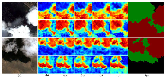
Figure 8.
Ablation heatmaps of cloud and cloud shadow which include (a) test image, (b) ResNet50, (c) ResNet50 + Swin, (d) ResNet50 + Swin + MAFM, (e) ResNet50 + Swin + MAFM + IDAM, (f) ResNet50 + Swin + MAFM + IDAM + RGM and (g) label.
3.6. Comparative Experiments on Different Datasets
In the subsequent comparative experiments, we compared our model with currently popular models based on CNN or transformers. The network structures or feature extraction methods of some networks are similar to ours. As a pure transformer model, PVT can automatically extract and encode critical features from an input sequence. Additionally, the PVT uses a multi-scale pyramid structure to effectively capture features at different scales. CVT integrates features extracted by convolution into the transformer, combining the local perceptual capability of CNN with the global perceptual capability of a transformer. Mpvit, BiseNetV2, and DBNet use a dual branch network to integrate detail information and semantic information, but their network structures are different. Both HRViT and CMT are hybrid models that combine CNN and transformers. CGNet utilizes a multi-scale contextual integration mechanism to enhance its segmentation capability in complex scenes. UNet uses a unique encoder and decoder structure that thoroughly fuses low-level and high-level features. SwinUNet, an UNet structure based on the Swin transformer, utilizes the advantages of UNet and the Swin transformer. DeepLabV3 and PSPNet use a pyramid pooling module (PPM) to capture multi-scale features, effectively enhancing the performance of large-scale image segmentation. HRNet uses multi-scale at the same feature level to combine fine and rough features. PAN uses a feature pyramid attention (FPA) to enhance the efficiency and accuracy of classification. CloudNet and CDUNet, specifically designed for cloud images, achieve notable results in detecting clouds and their shadows. As an advanced semantic segmentation model, OCRNet pays attention to object-level contextual information to enhance segmentation accuracy.
3.6.1. Comparison Test on Cloud and Cloud Shadow Dataset
To fully understand the effectiveness of our model, we designed comparative experiments on this dataset. Our model was compared with the current cutting-edge semantic segmentation technologies. To ensure the objectivity of the experiment, we set the experimental parameters to default values. Table 5 records the P (%), R (%), and (%) of cloud and cloud shadow categories, as well as the comprehensive metrics PA (%), MPA (%) and MIoU (%) of the comparison models. Table 5 also provides the time of training a picture (time) for each model as a direct measure of the model’s inference speed. In Table 5, the P (%) of the cloud category obtained using our model is slightly lower than that obtained using DBNet, but the R (%) and (%) of the cloud category obtained using our model reach optimal results. In cloud shadow detection, our model ranks ahead in P (%), R (%), and (%) among all models. Additionally, our model ranks ahead in PA (%) and achieves the best results in MPA (%) and MIoU (%). Notably, although our model combines ResNet50 and the Swin transformer, which results in high memory overhead, it only takes 19.33 ms to train a picture, ranking it as average in inference speed among all models.
Table 5.
Comparison of different models on Cloud and Cloud Dataset (bold represents the best result).
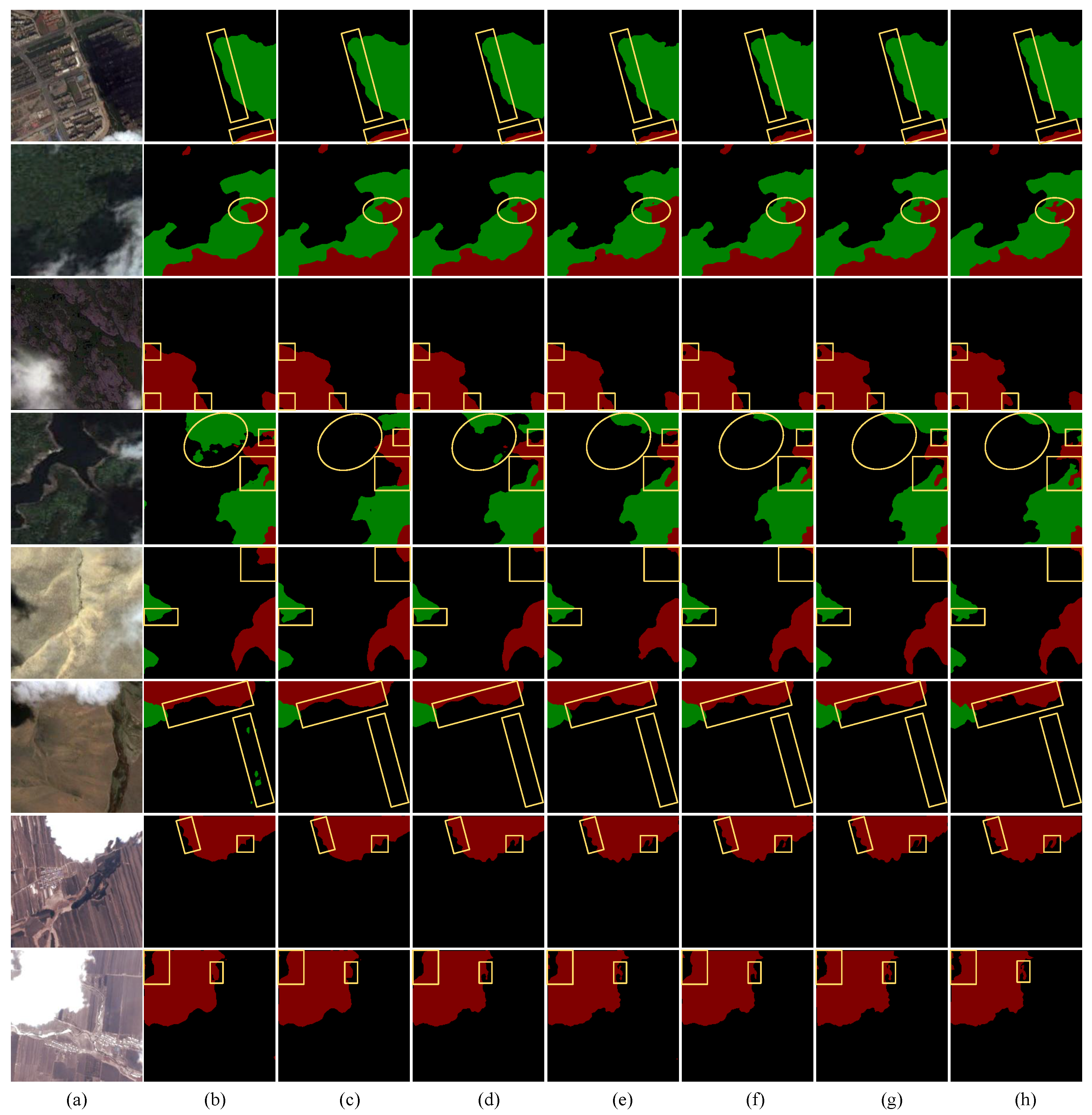
Figure 9 shows the semantic segmentation images of the top six models ranked by the MIoU metric. In Figure 9, the first three rows show the segmentation effect of an urban scene, a forest scene and a mountain scene, respectively. Our model performs well in the three scenes, effectively distinguishing the boundaries between clouds and background, as well as between cloud shadows and background. This is because the RGM in our model enhances the focus on boundary information, resulting in finer boundary segmentation. In Table 5, our model achieves of 95.13% for clouds and 93.37% for cloud shadows, respectively, which indicates its superior performance in segmenting boundaries of clouds and their shadows. The fourth row shows the segmentation effect of a shrub scene. In the fourth row, the elliptical frame highlights our model’s excellent recognition ability for cloud shadows and the two rectangular frames illustrate that our model precisely processes boundaries between different categories. In the drought scene of the fifth row and the canyon scene of the sixth row, the segmentation situation of our model is similar to the corresponding label. Since MAFM promotes the interaction of deep features at the same level and fully integrates local and global information, it enhances the boundary segmentation capabilities for clouds and their shadows and improves small target detection, thus achieving better classification. In Table 5, our model shows great cloud and cloud shadow detection capabilities with P (%) reaching 96.21% for cloud detection and 95.79% for cloud shadow detection. In the glacier scene of the seventh row and the snow scene of the eighth row, snow and clouds, which have similar colours and shapes, can easily be confused. Our model’s IDAM deeply aggregates multi-scale depth features, enhancing the recognition of small targets and preventing misidentification of snow on the ground as clouds. Compared to other methods, our model shows great performance in boundary repair and small target detection.
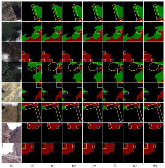
Figure 9.
Comparison of different models under different scenarios on Cloud and Cloud Shadow Dataset. (a) test image. (b) PAN. (c) HRNet. (d) DBNet. (e) OCRNet. (f) CDUNet. (g) MAFNet (ours). (h) label. Yellow circles and frames represent significant segmentation differences between different models.
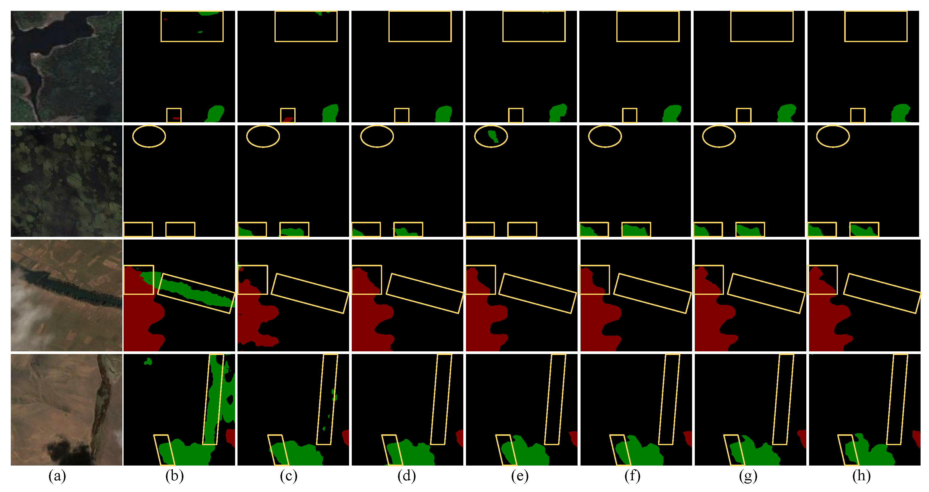
As shown in Figure 10, we also selected four scenes with severe false and missed detections for prediction comparison. In the first forest scenes, PAN and HRNet misclassify the background. In the second forest scenes, PAN fails to detect cloud shadows and OCRNet misclassifies the background as cloud shadows. In the third farmland scene, PAN has a high false detection rate for cloud shadows and HRNet has a high missed detection rate for clouds, while only our model achieves the most refined boundary segmentation between clouds and the background. In the fourth drought scene, PAN has a high false detection rate for cloud shadows and HRNet shows several missed detections of small target cloud shadows, while DBNet, OCRNet, CDUNet and our model demonstrate the excellent localization ability for clouds and cloud shadows. PAN and HRNet contain a large number of CNN structures, which suppresses the model’s global perception ability. This suppression causes the model to ignore regions with high similarity, resulting in false and missed detections of clouds and shadows. DBNet uses a dual-branch network to extract features, which is very effective for cloud detection. In Table 5, DBNet achieves the highest P (%) for the cloud category at 96.22%. As a CNN-based structure, OCRNet extracts object-level context information, but it still lacks the extraction of global features. CDUNet, a method specifically for the cloud and cloud shadow detection, utilizes excellent detail extraction capabilities to detect and process the distribution of cloud shadows. The P (%), R (%) and (%) of CDUNet for cloud shadows are the highest, at 97.94%, 97.39% and 96.40%, respectively. However, the inference speed of CDUNet is too slow, and the time metric of CDUNet is 32.15 ms. In our model, MAFM and IDAM enhance the ability to detect small targets, in addition to MAFM and RGM refining the boundary segmentation, resulting in our model achieving optimal classification results. Compared to DBNet and CDUNet, which combine CNN and a transformer, MAFNet exhibits significant advantages. Table 5 demonstrates the MIoU (%) of our model reaches the maximum value of 93.67%, fully demonstrating our model’s powerful performance in detecting clouds and their shadows.
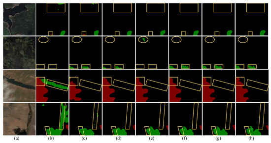
Figure 10.
False detection comparison of different models on Cloud and Cloud Shadow Dataset. (a) test images. (b) PAN. (c) HRNet. (d) DBNet. (e) OCRNet. (f) CDUNet. (g) MAFNet (ours). (h) label. Yellow circles and frames represent significant segmentation differences between different models.
3.6.2. Generalization Experiment of HRC-WHU Dataset
Comparative experiments on this dataset were performed to test the generalization performance of our model. The parameters in the experiments were set to default values. The experimental results are shown in Table 6. Since we only selected two categories (cloud and background) for the comparative experiments, most models demonstrate their excellent performance. Compared to other networks, our model achieves the highest values in PA (%), MPA (%), R (%), and MIoU (%), which verifies the generalization capability of our model.
Table 6.
Comparison of different models on HRC-WHU dataset (bold represents the best result).
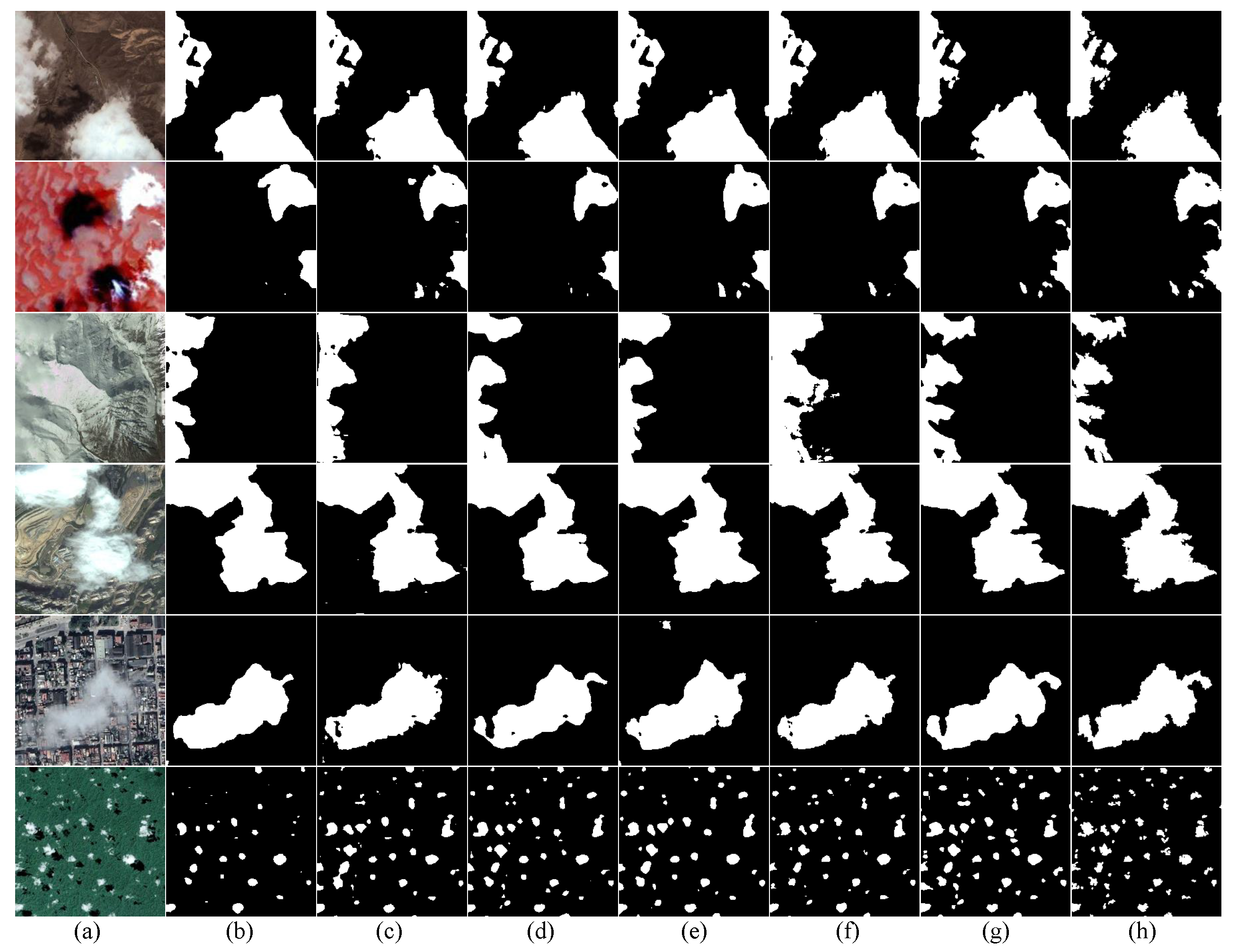
In Figure 11, we compared the prediction images of our network with the other five highest MIoU models. In the first row of a desert scene, each model’s classification situation is similar to the corresponding label, while our model has the most precise segmentation boundaries for clouds. In the second row of a floral garden scene, where the colour difference between clouds and background is large and easy to distinguish, our model accurately identifies the most clouds. In Table 6, the PA (%) of our model reaches the highest value of 98.59%, demonstrating our model’s capability for cloud detection. Accurate localization of thin clouds has always been a significant challenge in remote sensing images. In the third row of a hill scene, where the colours of thin clouds and the background are similar and difficult to distinguish, the other five models are notably weaker in the localization of thin cloud boundaries and the detection of small thin cloud targets compared to our model. In Table 6, the MPA (%) of our model reaches the highest value of 97.81%, indicating that our model is the best to differentiate between thin clouds and the background. This is because MAFM and RGM enhance attention to similar regions, improving the ability to distinguish clouds. In the fourth row of a mountain scene, our model achieves more precise boundary segmentation. In the fifth row of an urban scene, our model has strong thin cloud localization capability. Table 6 displays our model’s R (%) reaches the highest value of 98.19%, fully demonstrating high sensitivity of our model to thin clouds. In the sixth row of a forest scene, there are many small cloud targets that are prone to false and missed detection. Because MAFM and IDAM improve the recognition ability for small targets, Our model accurately localizes the small cloud targets. In summary, on the HRC-WHU dataset, our model outperforms other models in small target localization, boundary segmentation, and other aspects.
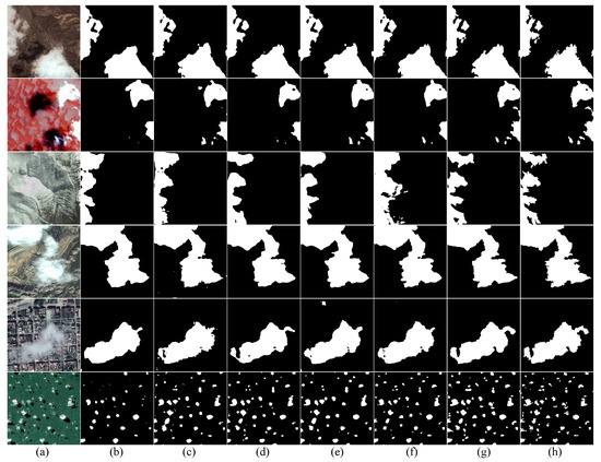
Figure 11.
Comparison of different models under different scenarios on HRC-WHU Dataset. (a) test images. (b) HRNet. (c) CVT. (d) OCRNet. (e) DBNet. (f) CDUNet. (g) MAFNet (ours). (h) label.
3.6.3. Generalization Experiment of SPARCS Dataset
We continued with comparative experiments using the SPARCS 7 classification dataset to additionally verify our model’s generalization capability. Table 7 displays comparison results. Class pixel accuracy represents the P (%) for each category. Our model achieves the highest values in the comprehensive metrics (%) and MIoU (%), indicating our model’s advantage in the multi-class detection. In addition, the P (%) for the land category and P (%) for the snow category reach the highest utilizing our model, which indicates that MAFNet has high applicability in snow and land scenes. The P (%) of our model for the cloud category is slightly lower than that of UNet, which achieves the highest P (%) for the cloud category. The P(%) of our model for the cloud shadow category is only second to the that of CGNet.
Table 7.
Comparison of different models on the SPARCS dataset (bold represents the best result).
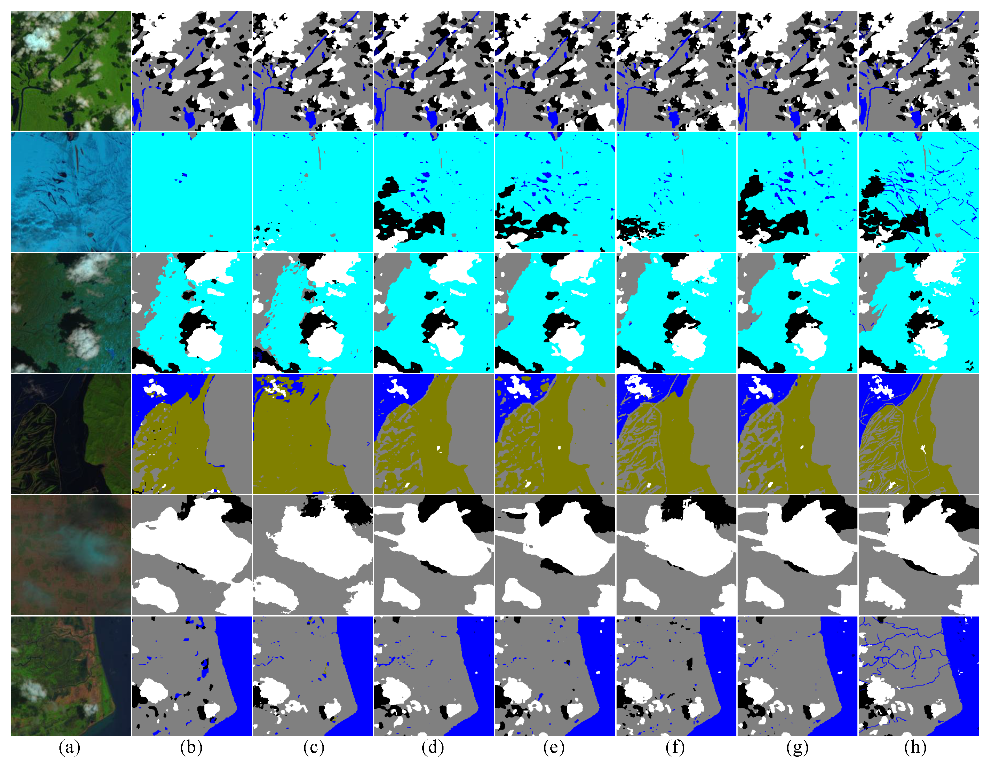
In Figure 12, we compared, the prediction images of our network with the other five highest MIoU models. The first line displays the classification situation of the cloud, cloud shadow, water, land and shadow over water categories. Few omissions and misjudgments appears at the real segmentation boundaries between the five categories if our model is used. In Table 7, our model’s (%) reaches the highest value of 84.95%, demonstrating its excellent ability to repair boundaries between different categories. The second and third lines display the classification situation of the snow, water, cloud, cloud shadow and land categories. Our model detects more clouds and their shadows and exhibits the strongest detection capabilities for the snow and land categories. In Table 7, the P (%) of our model for the snow and land category are the highest at 96.99% and 97.11%,respectively, indicating our model’s excellent discrimination ability for the snow and land categories. The fourth line displays the classification situation for the cloud, water, land, and flood categories. Our model demonstrates superior performance in detecting small cloud targets. The fifth line displays the classification situation for the cloud, cloud shadow and land categories. Since the colour of the original image is dark, non-cloud shadows are easily misclassified as cloud shadows. However, our model exhibits excellent discrimination capability for cloud shadows, with no large-scale omissions and misjudgments for the cloud shadow category. As shown in Table 7, the P (%) of our model for the cloud shadow reaches 80.87% and ranks second. The sixth row demonstrates the classification situation for the cloud, cloud shadow, water, and land categories. Our model demonstrates the most precise boundary segmentation for the water and land categories. In summary, our model performs better than other networks in cloud and cloud shadow detection, small target detection, and boundary repair. This is mainly because combining CNN with a transformer effectively integrates global and detailed information, MAFM and RGM contribute to more refined segmentation boundaries, and MAFM and IDAM enhance the network’s focus on small targets.
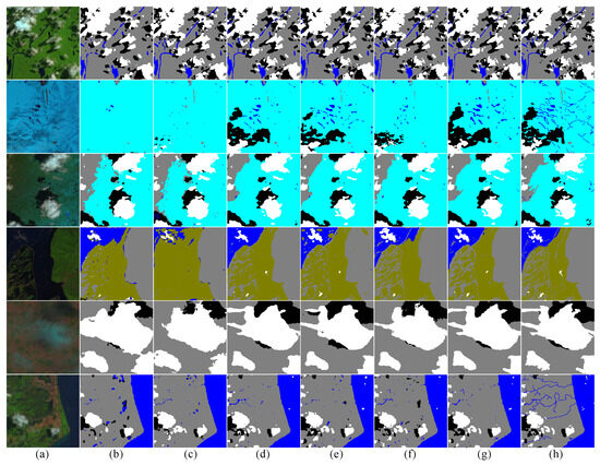
Figure 12.
Comparison of different models under different scenarios on SPARCS Dataset. (a) test images. (b) Mpvit. (c) DBNet. (d) DeepLabV3. (e) OCRNet. (f) CDUNet. (g) MAFNet (ours). (h) label.
4. Conclusions
This paper proposed a multi-branch attention fusion network (MAFNet). In the encoder section, we utilized the advantages of ResNet50 in extracting detailed information and Swin transformer in extracting global information. To achieve full fusion of the local information and global information, we designed a multi-branch attention fusion module (MAFM), thereby enhancing boundary segmentation and improving small target detection. To enhance the detection accuracy of small targets, we introduced an information deep aggregation module (IDAM), which extracts multi-scale deep features and performs deep aggregation, increasing the sensitivity to small targets. To make the segmentation boundaries finer, we designed a recover guided module (RGM) in the decoder section to adjust the attention distribution of the network on feature maps, enhancing the network’s focus on boundary information. Experiments display that the MAFNet outperforms other networks on Cloud and Cloud Shadow dataset, HRC-WHU dataset, and SPARCS dataset. In the future, we will apply the network to other remote sensing images, making the network widely applicable for cloud detection. Additionally, we will attempt to make the network more lightweight for less memory overhead.
Author Contributions
Conceptualization, H.G. and G.G.; methodology, Y.L.; software, H.G.; validation, Y.L. and H.L.; formal analysis, G.G.; investigation, H.G. and Y.X.; resources, Y.L.; data curation, Y.X.; writing—original draft preparation, H.G.; writing—review and editing, Y.L.; visualization, H.G.; supervision, Y.L.; project administration, Y.L.; funding acquisition, Y.L. All authors have read and agreed to the published version of the manuscript.
Funding
This work is supported in part by the National Natural Science Foundation of PR China (42075130).
Data Availability Statement
Data are contained within the article.
Conflicts of Interest
The authors declare no conflicts of interest.
References
- Zhu, Z.; Woodcock, C.E. Object-based cloud and cloud shadow detection in Landsat imagery. Remote Sens. Environ. 2012, 118, 83–94. [Google Scholar] [CrossRef]
- Manolakis, D.G.; Shaw, G.A.; Keshava, N. Comparative analysis of hyperspectral adaptive matched filter detectors. In Proceedings of the Algorithms for Multispectral, Hyperspectral, and Ultraspectral Imagery VI, Orlando, FL, USA, 24–26 April 2000; SPIE: Bellingham, WA, USA, 2000; Volume 4049, pp. 2–17. [Google Scholar]
- Zhai, H.; Zhang, H.; Zhang, L.; Li, P. Cloud/shadow detection based on spectral indices for multi/hyperspectral optical remote sensing imagery. ISPRS J. Photogramm. Remote Sens. 2018, 144, 235–253. [Google Scholar] [CrossRef]
- Kegelmeyer, W., Jr. Extraction of Cloud Statistics from Whole Sky Imaging Cameras; Technical Report; Sandia National Lab. (SNL-CA): Livermore, CA, USA, 1994. [Google Scholar]
- Cheng, G.; Wang, Y.; Xu, S.; Wang, H.; Xiang, S.; Pan, C. Automatic Road Detection and Centerline Extraction via Cascaded End-to-End Convolutional Neural Network. IEEE Trans. Geosci. Remote Sens. 2017, 55, 3322–3337. [Google Scholar] [CrossRef]
- Song, L.; Xia, M.; Jin, J.; Qian, M.; Zhang, Y. SUACDNet: Attentional change detection network based on siamese U-shaped structure. Int. J. Appl. Earth Obs. Geoinf. 2021, 105, 102597. [Google Scholar] [CrossRef]
- Krizhevsky, A.; Sutskever, I.; Hinton, G.E. ImageNet Classification with Deep Convolutional Neural Networks. In Advances in Neural Information Processing Systems 25, Proceedings of the 26th Annual Conference on Neural Information Processing Systems 2012, Lake Tahoe, NV, USA, 3–6 December 2012; Pereira, F., Burges, C., Bottou, L., Weinberger, K., Eds.; Curran Associates, Inc.: Nice, France, 2012; Volume 25. [Google Scholar]
- Simonyan, K.; Zisserman, A. Very deep convolutional networks for large-scale image recognition. arXiv 2014, arXiv:1409.1556. [Google Scholar]
- He, K.; Zhang, X.; Ren, S.; Sun, J. Deep residual learning for image recognition. In Proceedings of the IEEE Conference on Computer Vision and Pattern Recognition, Las Vegas, NV, USA, 26 June–1 July 2016; pp. 770–778. [Google Scholar]
- Long, J.; Shelhamer, E.; Darrell, T. Fully convolutional networks for semantic segmentation. In Proceedings of the IEEE Conference on Computer Vision and Pattern Recognition, Boston, MA, USA, 7–12 June 2015; pp. 3431–3440. [Google Scholar]
- Ronneberger, O.; Fischer, P.; Brox, T. U-net: Convolutional networks for biomedical image segmentation. In Proceedings of the International Conference on Medical Image Computing and Computer-Assisted Intervention, Munich, Germany, 5–9 October 2015; pp. 234–241. [Google Scholar]
- Zhao, H.; Shi, J.; Qi, X.; Wang, X.; Jia, J. Pyramid scene parsing network. In Proceedings of the IEEE Conference on Computer Vision and Pattern Recognition, Honolulu, HI, USA, 21–26 July 2017; pp. 2881–2890. [Google Scholar]
- Yu, C.; Wang, J.; Peng, C.; Gao, C.; Yu, G.; Sang, N. BiSeNet: Bilateral Segmentation Network for Real-time Semantic Segmentation. In Proceedings of the European Conference on Computer Vision (ECCV), Munich, Germany, 8–14 September 2018. [Google Scholar]
- Gu, J.; Kwon, H.; Wang, D.; Ye, W.; Li, M.; Chen, Y.H.; Lai, L.; Chandra, V.; Pan, D.Z. Multi-Scale High-Resolution Vision Transformer for Semantic Segmentation. In Proceedings of the IEEE/CVF Conference on Computer Vision and Pattern Recognition (CVPR), New Orleans, LA, USA, 18–24 June 2022; pp. 12094–12103. [Google Scholar]
- Yu, C.; Xiao, B.; Gao, C.; Yuan, L.; Zhang, L.; Sang, N.; Wang, J. Lite-HRNet: A Lightweight High-Resolution Network. In Proceedings of the IEEE/CVF Conference on Computer Vision and Pattern Recognition (CVPR), Nashville, TN, USA, 20–25 June 2021; pp. 10440–10450. [Google Scholar]
- Chen, L.C.; Papandreou, G.; Kokkinos, I.; Murphy, K.; Yuille, A.L. DeepLab: Semantic Image Segmentation with Deep Convolutional Nets, Atrous Convolution, and Fully Connected CRFs. IEEE Trans. Pattern Anal. Mach. Intell. 2018, 40, 834–848. [Google Scholar] [CrossRef]
- Dong, R.; Pan, X.; Li, F. DenseU-net-based semantic segmentation of small objects in urban remote sensing images. IEEE Access 2019, 7, 65347–65356. [Google Scholar] [CrossRef]
- Chen, X.; Li, Z.; Jiang, J.; Han, Z.; Deng, S.; Li, Z.; Fang, T.; Huo, H.; Li, Q.; Liu, M. Adaptive Effective Receptive Field Convolution for Semantic Segmentation of VHR Remote Sensing Images. IEEE Trans. Geosci. Remote Sens. 2021, 59, 3532–3546. [Google Scholar] [CrossRef]
- Carion, N.; Massa, F.; Synnaeve, G.; Usunier, N.; Kirillov, A.; Zagoruyko, S. End-to-End Object Detection with Transformers. In Proceedings of the Computer Vision—ECCV 2020, Glasgow, UK, 23–28 August 2020; Vedaldi, A., Bischof, H., Brox, T., Frahm, J.M., Eds.; Springer: Cham, Switzerland, 2020; pp. 213–229. [Google Scholar]
- Dosovitskiy, A.; Beyer, L.; Kolesnikov, A.; Weissenborn, D.; Zhai, X.; Unterthiner, T.; Dehghani, M.; Minderer, M.; Heigold, G.; Gelly, S.; et al. An image is worth 16 × 16 words: Transformers for image recognition at scale. arXiv 2020, arXiv:2010.11929. [Google Scholar]
- Liu, Z.; Lin, Y.; Cao, Y.; Hu, H.; Wei, Y.; Zhang, Z.; Lin, S.; Guo, B. Swin transformer: Hierarchical vision transformer using shifted windows. In Proceedings of the IEEE/CVF International Conference on Computer Vision, Montreal, BC, Canada, 11–17 October 2021; pp. 10012–10022. [Google Scholar]
- Wang, W.; Xie, E.; Li, X.; Fan, D.P.; Song, K.; Liang, D.; Lu, T.; Luo, P.; Shao, L. Pyramid Vision Transformer: A Versatile Backbone for Dense Prediction without Convolutions. In Proceedings of the IEEE/CVF International Conference on Computer Vision (ICCV), Montreal, BC, Canada, 11–17 October 2021; pp. 568–578. [Google Scholar]
- Wu, H.; Xiao, B.; Codella, N.; Liu, M.; Dai, X.; Yuan, L.; Zhang, L. CvT: Introducing Convolutions to Vision Transformers. In Proceedings of the IEEE/CVF International Conference on Computer Vision (ICCV), Montreal, BC, Canada, 11–17 October 2021; pp. 22–31. [Google Scholar]
- Lu, C.; Xia, M.; Qian, M.; Chen, B. Dual-branch network for cloud and cloud shadow segmentation. IEEE Trans. Geosci. Remote Sens. 2022, 60, 5410012. [Google Scholar] [CrossRef]
- Gu, G.; Weng, L.; Xia, M.; Hu, K.; Lin, H. Muti-path Muti-scale Attention Network for Cloud and Cloud shadow segmentation. IEEE Trans. Geosci. Remote Sens. 2024, 62, 5404215. [Google Scholar] [CrossRef]
- Wu, C.; Wu, F.; Huang, Y. Da-transformer: Distance-aware transformer. arXiv 2020, arXiv:2010.06925. [Google Scholar]
- Song, L.; Xia, M.; Weng, L.; Lin, H.; Qian, M.; Chen, B. Axial cross attention meets CNN: Bibranch fusion network for change detection. IEEE J. Sel. Top. Appl. Earth Obs. Remote Sens. 2022, 16, 21–32. [Google Scholar] [CrossRef]
- He, X.; Zhou, Y.; Zhao, J.; Zhang, D.; Yao, R.; Xue, Y. Swin transformer embedding for remote sensing image semantic segmentation. IEEE Trans. Geosci. Remote Sens. 2022, 60, 4408715. [Google Scholar] [CrossRef]
- Chaman, A.; Dokmanic, I. Truly shift-invariant convolutional neural networks. In Proceedings of the IEEE/CVF Conference on Computer Vision and Pattern Recognition, Nashville, TN, USA, 20–25 June 2021; pp. 3773–3783. [Google Scholar]
- Li, B.; Dai, Y.; Cheng, X.; Chen, H.; Lin, Y.; He, M. Skeleton based action recognition using translation-scale invariant image mapping and multi-scale deep CNN. In Proceedings of the 2017 IEEE International Conference on Multimedia & Expo Workshops (ICMEW), Hong Kong, 10–14 July 2017; pp. 601–604. [Google Scholar]
- Ha, S.; Yun, J.M.; Choi, S. Multi-modal convolutional neural networks for activity recognition. In Proceedings of the 2015 IEEE International Conference on Systems, Man, and Cybernetics, Kowloon Tong, Hong Kong, 9–12 October 2015; pp. 3017–3022. [Google Scholar]
- Hu, K.; Zhang, D.; Xia, M. CDUNet: Cloud detection UNet for remote sensing imagery. Remote Sens. 2021, 13, 4533. [Google Scholar] [CrossRef]
- Woo, S.; Park, J.; Lee, J.Y.; Kweon, I.S. Cbam: Convolutional block attention module. In Proceedings of the European Conference on Computer Vision (ECCV), Munich, Germany, 8–14 September 2018; pp. 3–19. [Google Scholar]
- Li, Z.; Shen, H.; Cheng, Q.; Liu, Y.; You, S.; He, Z. Deep learning based cloud detection for medium and high resolution remote sensing images of different sensors. ISPRS J. Photogramm. Remote Sens. 2019, 150, 197–212. [Google Scholar] [CrossRef]
- Hughes, M.J.; Hayes, D.J. Automated detection of cloud and cloud shadow in single-date Landsat imagery using neural networks and spatial post-processing. Remote Sens. 2014, 6, 4907–4926. [Google Scholar] [CrossRef]
- Wu, T.; Tang, S.; Zhang, R.; Cao, J.; Zhang, Y. Cgnet: A light-weight context guided network for semantic segmentation. IEEE Trans. Image Process. 2020, 30, 1169–1179. [Google Scholar] [CrossRef]
- Lee, Y.; Kim, J.; Willette, J.; Hwang, S.J. Mpvit: Multi-path vision transformer for dense prediction. In Proceedings of the IEEE/CVF Conference on Computer Vision and Pattern Recognition, New Orleans, LA, USA, 18–24 June 2022; pp. 7287–7296. [Google Scholar]
- Illingworth, A.; Hogan, R.; O’connor, E.; Bouniol, D.; Brooks, M.; Delanoë, J.; Donovan, D.; Eastment, J.; Gaussiat, N.; Goddard, J.; et al. Cloudnet: Continuous evaluation of cloud profiles in seven operational models using ground-based observations. Bull. Am. Meteorol. Soc. 2007, 88, 883–898. [Google Scholar] [CrossRef]
- Chen, L.C.; Zhu, Y.; Papandreou, G.; Schroff, F.; Adam, H. Encoder-decoder with atrous separable convolution for semantic image segmentation. In Proceedings of the European Conference on Computer Vision (ECCV), Munich, Germany, 8–14 September 2018; pp. 801–818. [Google Scholar]
- Yu, C.; Gao, C.; Wang, J.; Yu, G.; Shen, C.; Sang, N. Bisenet v2: Bilateral network with guided aggregation for real-time semantic segmentation. Int. J. Comput. Vis. 2021, 129, 3051–3068. [Google Scholar] [CrossRef]
- Guo, J.; Han, K.; Wu, H.; Tang, Y.; Chen, X.; Wang, Y.; Xu, C. Cmt: Convolutional neural networks meet vision transformers. In Proceedings of the IEEE/CVF Conference on Computer Vision and Pattern Recognition, New Orleans, LA, USA, 18–24 June 2022; pp. 12175–12185. [Google Scholar]
- Cao, H.; Wang, Y.; Chen, J.; Jiang, D.; Zhang, X.; Tian, Q.; Wang, M. Swin-unet: Unet-like pure transformer for medical image segmentation. In Proceedings of the European Conference on Computer Vision, Tel Aviv, Israel, 23–27 October 2022; pp. 205–218. [Google Scholar]
- Li, H.; Xiong, P.; An, J.; Wang, L. Pyramid attention network for semantic segmentation. arXiv 2018, arXiv:1805.10180. [Google Scholar]
- KO, M.A.; Poruran, S. OCR-nets: Variants of pre-trained CNN for Urdu handwritten character recognition via transfer learning. Procedia Comput. Sci. 2020, 171, 2294–2301. [Google Scholar] [CrossRef]
Disclaimer/Publisher’s Note: The statements, opinions and data contained in all publications are solely those of the individual author(s) and contributor(s) and not of MDPI and/or the editor(s). MDPI and/or the editor(s) disclaim responsibility for any injury to people or property resulting from any ideas, methods, instructions or products referred to in the content. |
© 2024 by the authors. Licensee MDPI, Basel, Switzerland. This article is an open access article distributed under the terms and conditions of the Creative Commons Attribution (CC BY) license (https://creativecommons.org/licenses/by/4.0/).