Article

Post-Logging Canopy Gap Dynamics and Forest Regeneration Assessed Using Airborne LiDAR Time Series in the Brazilian Amazon with Attribution to Gap Types and Origins

by
Philip Winstanley
1,
Ricardo Dalagnol
1,2,3,4,*,
Sneha Mendiratta
1,
Daniel Braga
5,
Lênio Soares Galvão
5 and
Polyanna da Conceição Bispo
1
1
Department of Geography, School of Environment Education and Development, University of Manchester, Manchester M13 9PL, UK
2
Center for Tropical Research, Institute of the Environment and Sustainability, University of California, Los Angeles–UCLA, Los Angeles, CA 90095, USA
3
NASA-Jet Propulsion Laboratory, California Institute of Technology, Pasadena, CA 91109, USA
4
CTrees, Pasadena, CA 91105, USA
5
Earth Observation and Geoinformatics Division, National Institute for Space Research-INPE, São José dos Campos 12227-010, Brazil
*
Author to whom correspondence should be addressed.
Remote Sens. 2024, 16(13), 2319; https://doi.org/10.3390/rs16132319
Submission received: 24 April 2024 / Revised: 4 June 2024 / Accepted: 21 June 2024 / Published: 25 June 2024
(This article belongs to the Special Issue New Methods and Applications in Remote Sensing of Tropical Forests)

Abstract

:
Gaps are openings within tropical forest canopies created by natural or anthropogenic disturbances. Important aspects of gap dynamics that are not well understood include how gaps close over time and their potential for contagiousness, indicating whether the presence of gaps may or may not induce the creation of new gaps. This is especially important when we consider disturbances from selective logging activities in rainforests, which take away large trees of high commercial value and leave behind a forest full of gaps. The goal of this study was to quantify and understand how gaps open and close over time within tropical rainforests using a time series of airborne LiDAR data, attributing observed processes to gap types and origins. For this purpose, the Jamari National Forest located in the Brazilian Amazon was chosen as the study area because of the unique availability of multi-temporal small-footprint airborne LiDAR data covering the time period of 2011–2017 with five data acquisitions, alongside the geolocation of trees that were felled by selective logging activities. We found an increased likelihood of natural new gaps opening closer to pre-existing gaps associated with felled tree locations (<20 m distance) rather than farther away from them, suggesting that small-scale disturbances caused by logging, even at a low intensity, may cause a legacy effect of increased mortality over six years after logging due to gap contagiousness. Moreover, gaps were closed at similar annual rates by vertical and lateral ingrowth (16.7% yr−1) and about 90% of the original gap area was closed at six years post-disturbance. Therefore, the relative contribution of lateral and vertical growth for gap closure was similar when consolidated over time. We highlight that aboveground biomass or carbon density of logged forests can be overestimated if considering only top of the canopy height metrics due to fast lateral ingrowth of neighboring trees, especially in the first two years of regeneration where 26% of gaps were closed solely by lateral ingrowth, which would not translate to 26% of regeneration of forest biomass. Trees inside gaps grew 2.2 times faster (1.5 m yr−1) than trees at the surrounding non-gap canopy (0.7 m yr−1). Our study brings new insights into the processes of both the opening and closure of forest gaps within tropical forests and the importance of considering gap types and origins in this analysis. Moreover, it demonstrates the capability of airborne LiDAR multi-temporal data in effectively characterizing the impacts of forest degradation and subsequent recovery.

1. Introduction

The Amazon rainforest, a global biodiversity hotspot with an estimated 16,000 tree species [1], plays a crucial role as the most prominent land carbon sink worldwide [2]. Recent studies have pointed out that the Amazon is transforming into more of a carbon source than a sink due to elevated anthropogenic disturbances and intervention—mainly associated with deforestation [3]. Other anthropogenic disturbances that affect very large areas but do not change land use include logging and fire [4,5]. Moreover, studies also point out that the effects of degradation due to logging and fire activities have been surpassing the deforested area in the last decades [6]. The remaining degraded forests are left in a disturbed state, which may lead to increased tree mortality due to edge and fragmentation effects [5,7].
A forest that experienced disturbances from logging is left to recover with an increased number of gaps in its canopy [8]. A gap is defined as a hole in the forest extending down all levels [9]. It can be formed in different ways, such as from natural disturbances (e.g., windthrows or lightning), background tree mortality boosted by certain environmental factors (e.g., water-related stress or soil fertility), or anthropogenic sources such as logging, fire, and edge effects [10,11,12]. Nevertheless, gaps play a key role in the dynamics of a tropical forest. Gaps provide an environment that has different resource levels to the surrounding canopy, with increased light levels that provide colonization sites for shade-intolerant species [13,14].
A key part of understanding how forest dynamics work relies on the ability to map and quantify the gap dynamics. Gaps can be measured in different ways, starting at the most basic level through field campaigns and survey methods [9,15,16], up to more technological ways through remotely sensed light detection and ranging (LiDAR)-derived data, collected from terrestrial or airborne platforms [12,17]. The airborne LiDAR data provide a 3D representation of a gap through the point cloud [18], which allows for easier high-resolution mapping of many forest attributes including gaps [19,20,21]. Furthermore, the most common way to analyze gaps is through the calculation of canopy height models (CHMs), considering height thresholds to define a gap ranging from 4 to 20 m above ground [17,22,23]. More dynamic measurements of gaps have also been proposed, adapting thresholds to the studied forest site or a relative threshold based on a zonal maximum local height [12,24]. Nevertheless, whilst the use of LiDAR to map gaps is now very much commonplace in understanding the structure of canopies, the use of repeated LiDAR data to map canopy changes over an extended period is something that has been shown in a few papers but not extensively evaluated [25,26].
Several studies are looking at various gap properties such as gap size, extent, fraction, and distribution of gap sizes in the literature [17,26,27,28]. However, there are not many studies looking into the mode of gap closure, whether it is predominantly closed by vertical growth or lateral ingrowth of neighboring trees, and how existing gaps can potentially contribute to the opening of new gaps through contagion [29]. The first point is important because if gaps are predominantly closed by the lateral or horizontal encroachment of neighboring trees [17,26,30], this means that remote sensing approaches measuring forest structure and carbon from a bird’s eye can potentially overestimate its estimates. The second point is important because, although gap contagion and spreading of gaps has been studied as early as the 1980s, it is still in contention as to the presence of such a contagion effect between gaps [17] or its absence [29]. Similarly to edge effects that occur at the borders of the forest [5,7,31,32], the gap contagiousness may be an important mechanism of tree mortality. This could be especially important in the largely degraded areas of the southeast Amazon from which gap fraction and tree mortality have been estimated to be higher than the recorded values in the other Amazonian regions [12].
In this study, our goal was to quantify post-logging gap dynamics and forest regeneration within gaps in a tropical forest located in the Brazilian Amazon, with attribution to gap types and origins. Specifically, we aimed to (1) identify and analyze the formation and closure of forest gaps over time; (2) compare the rate of growth within gaps to the rate of growth in the nominally undisturbed forest canopy and estimate rates of lateral and vertical growth; and (3) assess whether the proximity to existing gaps contributed to the formation of new gaps. To do this, a time series of airborne LiDAR and field datasets were analyzed over the Jamari National Forest in the Brazilian Amazon. The availability of an airborne LiDAR dataset that spans from 2011 to 2017 and precise ground data recorded for selectively logged trees within the forest in 2010 and 2011 provided a great opportunity to study the gap dynamics with logging. First, the temporal changes in gaps were analyzed to assess both gap opening and closure. Then, growth was calculated, and a linear regression model was fitted to relate the vegetation’s initial height with expected growth. Finally, we applied a spatial analysis technique to test whether there was a significant spatial relationship in the gap creation process, rejecting or supporting the gap contagiousness theory, according to different gap types and origins.

2. Materials and Methods
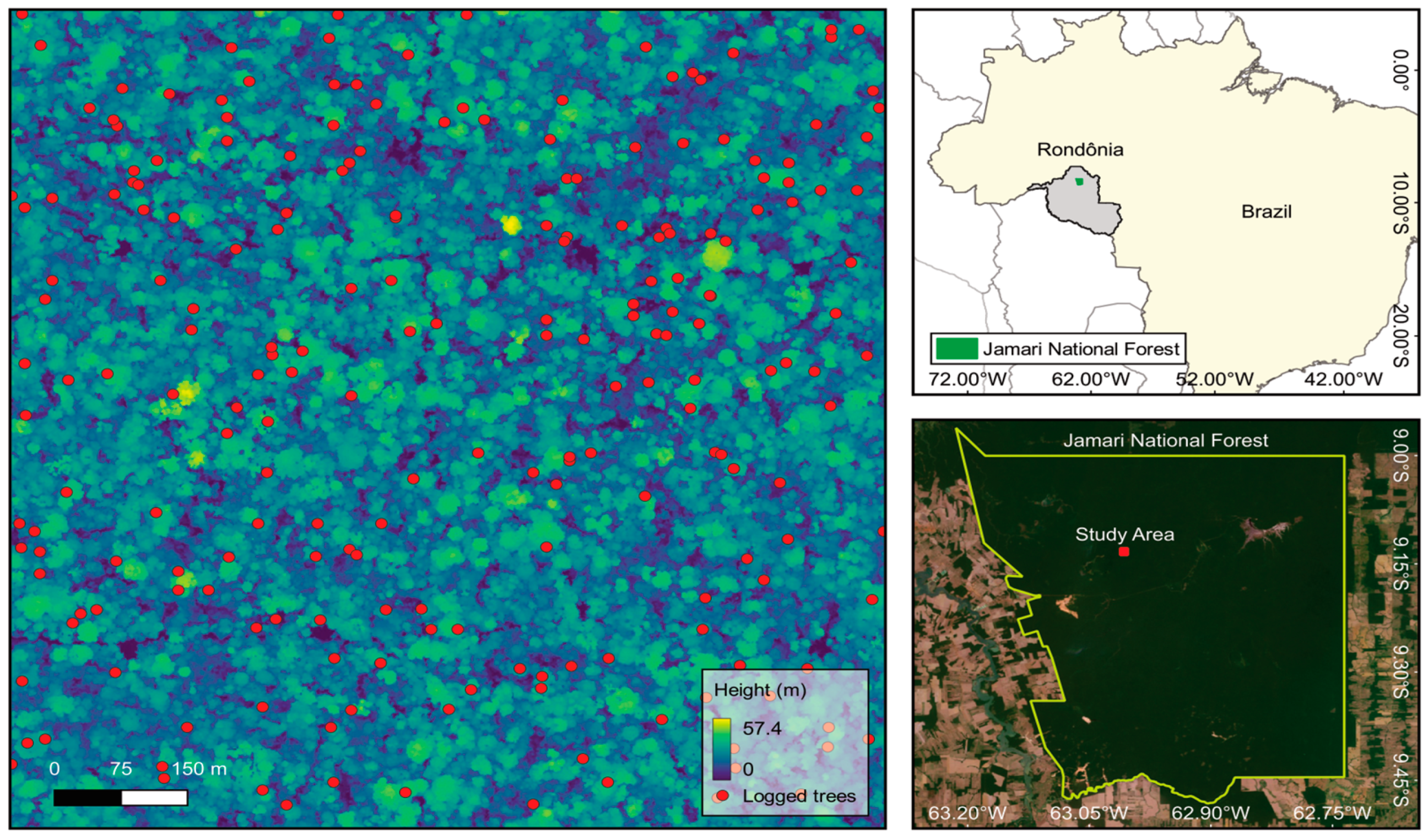
2.1. Study Area

The study area is located in the Jamari National Forest (09°10′S, 63°010′W), in the Brazilian state of Rondônia, in the southwest of Amazon rainforests (Figure 1). The vegetation covers an area of over 220,000 hectares, predominantly composed of lowland ombrophilous open forests [33]. The Jamari National Forest has a rainy tropical climate of hot humidity with an average temperature of 25 °C. The region has well-defined wet and dry seasons, with the wet season lasting from December to May and the dry season extending from June to November. The average rainfall in the study is approximately 2200 mm year−1 [34]. The Jamari National Forest has had 44% of its territory allocated for selective logging activities since 2008, with the logging activities being managed by the Brazilian Institute of Environment and Renewable Mineral Resources (IBAMA) and the Brazilian Forest Service. After extraction, the managed areas are left to recover naturally for 25 years [26]. The study focuses on a forest area of 104.42 ha (approximately 1 × 1 km) located within the entitled production area (UPA-01), which was selectively logged between 2010 and 2011. This area was carefully chosen due to the availability of the multi-temporal acquisition of airborne LiDAR data as well as the tree-by-tree information of logged trees collected at the field. The field dataset was collected by the SAKURA IND company, which was the concessionaire of this area at the time. It provides geolocation information on each tree within the area, highlighting those that have been logged, as well as their identified species, the diameter at breast height (DBH), and estimated volume (m3). The UPA-01 had at least 38 species of trees of economic interest identified during the field data collection with DBH ranging between 35 and 271 cm. The mean DBH was 56 cm. The logging intensity in this area was 215 logged trees (1699 m3 of wood), totaling a relative extraction of 2 trees ha−1 and 16.3 m3 ha−1.

2.2. Multi-Temporal LiDAR Data

Airborne LiDAR data were obtained in 2011, 2013, 2014, 2015, and 2017 after logging activities for an overlapping area of 1 km2 in the UPA-01 area. They were acquired by a consortium between the Brazilian Forest Service and the Sustainable Landscapes Brazil Project (https://www.paisagenslidar.cnptia.embrapa.br/webgis/, accessed on 3 February 2021). All point clouds consisted of very high point densities with at least 12 ppm2 (Table 1). This is much greater than the minimum point density (4 ppm2), which is usually necessary to obtain reliable digital terrain models (DTMs) and canopy height models (CHMs) [35].
The LiDAR point cloud was processed from its raw data into a canopy height model (CHM). Firstly, the point clouds were clipped to the same extent using the lasclip function and tiled for faster processing using the lastile function from LAStools v3.1.1 [36]. The point clouds were classified into ground or vegetation classes using lasground, lasheight, and lasclassify functions, using default parameters [36]. The data were visually inspected for quality control to ensure points classified as ground and vegetation fell in the expected locations in the study area. To avoid potential issues coming from the different LiDAR acquisitions in the extracted DTM, we compared the ground points’ height of the different dates using the 2014 acquisition as a reference and adjusted the mean height of the clouds by subtracting or adding the difference to the point cloud from 2014. The point clouds from the multiple acquisitions were normalized in terms of elevation due to minor differences we observed between the acquisitions (less than 1 m), similar to those performed in a previous study [26]. After the normalization, all points were used to create a single consistent DTM to be used to normalize all elevation to height and create the CHMs. Unlike the vertical correction performed, it was not necessary to align the point clouds horizontally as no major shifts in large stable tree crowns could be observed in between acquisitions. Once all the point clouds had their height values adjusted, the ground points from all five acquisitions were merged to create a combined DTM with 1 × 1 m resolution using the lidR package v3.1.3 [37] from R language [38]. This DTM was used to normalize all point clouds using the normalise_height function from lidR, and then CHMs for each date were extracted at a 1 × 1 m grid with the grid_canopy function from lidR. All returns from the LiDAR collection were used to create the CHMs.

2.3. Gap Delineation

Two gap concepts were considered in this study, as follows: (1) static gaps, delineated using one LiDAR CHM, representing static open areas in the canopy at one point in time; and (2) dynamic gaps, calculated from differences between two CHMs, indicating canopy disturbances occurring between a period likely related to tree mortality or branch/crown damage [17]. Static gaps were defined as holes in the forest canopy that extended up to 10 m in height above the ground with at least an area of 10 m2. Whilst this differs from the common height threshold for a gap definition by Brokaw’s 2 m above ground, studies of gap dynamics using LiDAR in similar tropical forests show that gaps extend to much higher heights above ground than Brokaw’s limit [17]. Using the field coordinates of selectively logged trees in 2010/2011, we qualified the forest and gaps of the first LiDAR CHM (year 2011) into three classes, as follows: (i) natural gaps of at least 30 m away from selectively logged trees; (ii) gaps formed from selective logging in 2010/2011, situated no more than 30 m from selectively logged trees; and (iii) non-gaps, including the remaining forest canopy area not covered by gaps. Previous studies have shown that the match between the logged tree geolocations and airborne lidar data in this site had a horizontal accuracy of less than 20 m [26].
Dynamic gaps were defined as a negative height difference between two time periods greater or equal to 10 m with an area greater or equal to 10 m2 [17]. Previous studies associate these differences with the occurrence of treefalls or crown damage in the canopy [17,25,26]. The dynamic gaps were delineated by calculating the change, or the subtraction, between two LiDAR CHMs (∆CHM) of the four-time intervals: (i) 2011 to 2013, (ii) 2013 to 2014, (iii) 2014 to 2015, and (iv) 2015 to 2017.

2.4. Data Analysis

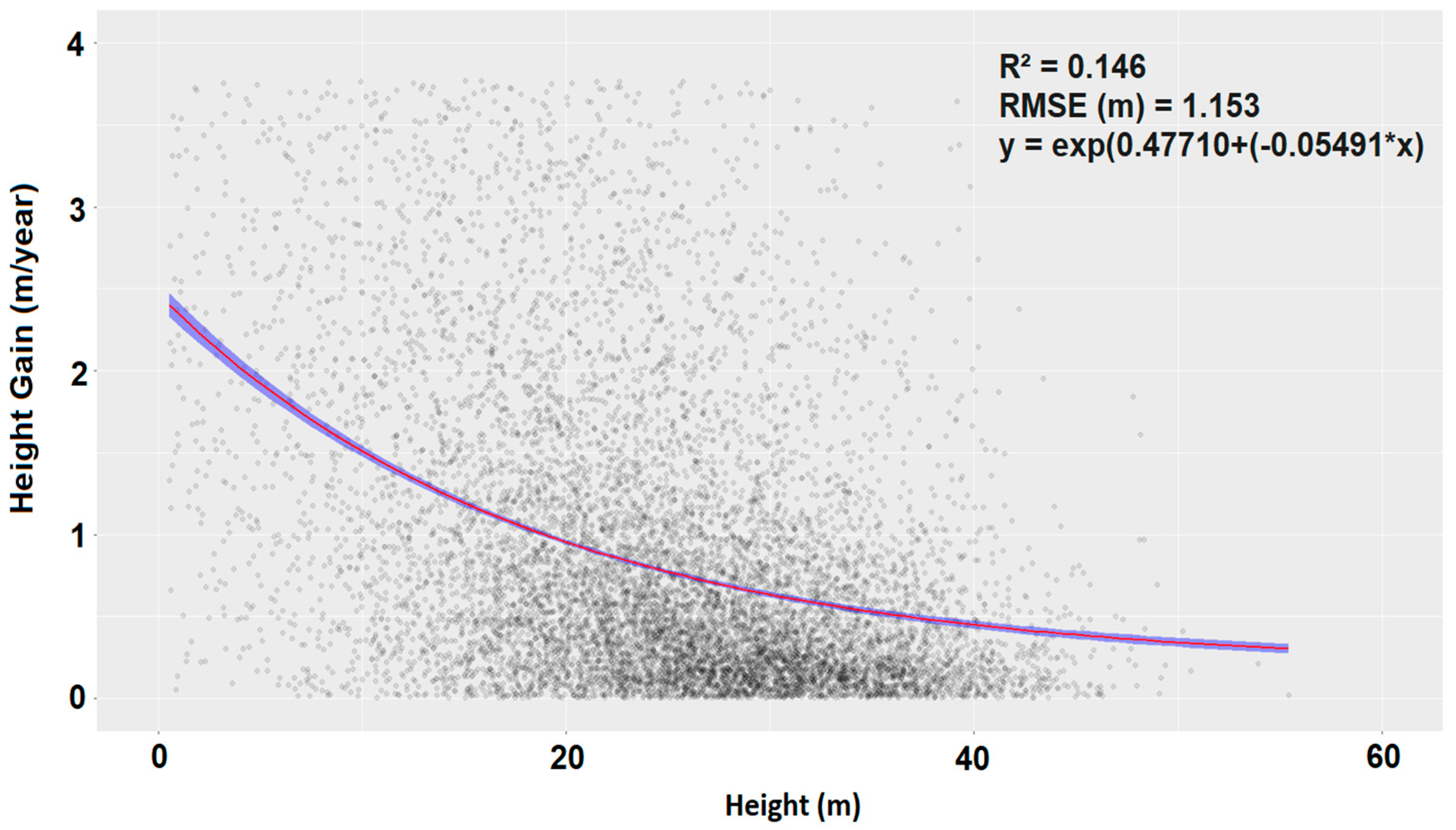
2.4.1. Lateral and Vertical Growth

Gaps can close over time due to the vertical growth of vegetation inside the gaps or lateral ingrowth of neighboring trees occupying the space. To disentangle vertical from lateral growth inside gaps, we used a method that assessed the maximum vertical growth of vegetation inside gaps [17,26]. The maximum vertical growth was defined as the mean plus three standard deviations of the mean height change inside the center of gaps between LiDAR acquisitions. To remove the influence of lateral ingrowth from this estimate, a negative buffer of −5 m was applied to each gap. Thus, only the center of gaps was used to calculate the maximum vertical growth and only gaps with a pre-buffer radius larger than 5 m (~78 m2 in the area) were used for this calculation. These are significantly larger sizes than the minimum gap size allowed by our definition (10 m2). This maximum vertical growth was then used to classify height change in gaps as either lateral (above the maximum growth) or vertical (below maximum growth) growth. Mean growth or height gain was calculated for each analyzed year. Furthermore, the 5th and 95th percentiles for vertical growth were also calculated, along with the number of gaps that were delineated.
We calculated statistics describing the number of new gaps formed between dates and existing gaps that were closed. New gaps formed were taken from the number of gaps delineated by the dynamic gaps, whilst existing gaps closed were calculated by comparing static gaps with the static gaps at the next LiDAR acquisition. If there was no intersection between a compared gap from the first and second date, then the gap was considered closed. These values were then normalized so that they represented opening and closure values per year. To visually represent the gap closure process, one gap was chosen to exemplify the changes in the gap due to lateral ingrowth between each acquisition from 2011 to 2017. Finally, we compared the vegetation growth between the three stratified classes (natural gaps, logged gaps, and non-gaps). Height change was calculated between pairs of subsequent CHM and values were filtered only for positive values below the maximum vertical growth.

2.4.2. Growth Model

To measure and understand how vegetation has grown in height inside gaps and at the forest canopy, a model was fitted using the current height and height gain between subsequent time periods derived from multi-temporal LiDAR data. We exclusively considered height gain values that were positive when calculating the ∆CHM values across all dates. After that, we sieved out the remaining values for lateral ingrowth by employing the maximum vertical growth value as done in previous studies [17,26]. The relationship between original height and height gain was quantified through a linear model, where the original height was used to predict the tree height gain per year. The exponential variable transformation was tested to improve data relationships. The model’s performance was verified with a determination coefficient (R2), root mean square error (RMSE), and relative RMSE (ratio between RMSE and mean observed height). To compare the mean vertical growth across the three classes, the mean value for growth was calculated and normalized to growth per year considering the time period between acquisitions. This provides three mean vertical growth values for each class calculated between the four acquisition periods, allowing for comparisons to be made between the classes. These values for growth were represented as box plots showing each of the three classes of gaps displayed for each of the periods between acquisitions. As part of the boxplot, notches were used to compare the medians of the values for 95% confidence intervals.

2.4.3. Gap Contagiousness

To determine whether there is a relationship between gap creation and proximity to pre-existing gaps, we performed three experiments with spatial analyses (Table 2). The first one looked at whether the distribution of static gaps from one date was associated in space with the newly created dynamic gaps of the next time period (“Static vs. Dynamic”). The second one tested whether there was a difference between natural or logging static gaps on the creation of dynamic gaps in the subsequent time period (“Gap type vs. Dynamic”). Finally, the third one verified whether the distribution of dynamic gaps from one time period was associated with newly created dynamic gaps in the next time period (“Dynamic vs. Dynamic”). For this purpose, the gap centroids were analyzed using the nncross function from the spatstat R package [39]. This function, given two-point patterns X and Y, finds the nearest neighbor in Y for each point of X. We then created a complete spatial randomness (CSR) envelope with a 1% significance level by running 199 Monte Carlo simulations of random (Poisson) point processes. This procedure was done using the Gcross function in the spatstat R package [40]. This allowed us to compare and determine whether the empirical distributions of distances were statistically different or not from random. If the cumulative distribution falls within the envelope, then the spatial pattern can be attributed to randomness; however, if the cumulative distribution lies above the 1% CSR envelope, then we can infer that the relationship between the two sets of points is clustered at that given distance.

3. Results

3.1. Gap Opening

For the analyzed time series (2011–2017), we observed the area occupied by gaps had maximum values in 2011 following the selective logging (mean area of 72.5 m2) and lowest values in 2017 (mean area of 43.2 m2) (Table 3). Overall, the total area of gaps steadily declined from 83,806 m2 in 2011 to 43,908 m2 in 2017, showing a 52.4% reduction in the total gap area of the study area. These correspond to a gap fraction of 8.4% in 2011 and 4.4% in 2017. The number of static gaps also declined over time but showed a slight increase in the last analyzed date. The increase in the number of static gaps over time, despite a reduction in their total area, can be attributed to various natural and anthropogenic factors. Tree falls due to age or strong winds lead to gaps, as do storms, lightning strikes, and fires that damage or kill trees. The probability of occurrence is influenced by environmental conditions—areas with higher wind speeds or more frequent storms are more likely to experience natural gap formation. Forest structure and composition also play a role; older forests with larger, mature trees may have more gaps due to tree falls, while younger, denser forests might have fewer but smaller gaps. Human activities, such as selective logging observed in the 2011 data, increase the likelihood of gap formation by removing specific trees.
The visual interpretation of the dynamic gaps over time highlighted the dynamism of these forests with high rates of gap openings in the different time intervals (Figure 2). When quantifying these gap openings, we noted a reduction in the static gap area from 2011 to 2017. However, the rates of dynamic gap creation and closure over time were highly variable and did not follow a clear pattern (Table 4). There was a higher number of new gaps formed per year than those that were closed, except in the 2014–2015 time period, where 191.8 new gaps were formed, while 321.5 gaps on average were closed.

3.2. Mode of Gap Closure and Tree Growth

We estimated a maximum vertical growth rate of 3.8 m yr−1 from 283 pixels of 1 × 1 m (or 283 m2 of gap area) located at the center of 15 gaps considering the ∆CHM between 2011 and 2013. Using this value as the threshold to differentiate lateral ingrowth and vertical growth, we estimated average vertical growth rates inside gaps ranging from 1.4 to 1.6 m yr−1 (Supplementary Table S1).
As the mechanisms of gap closure, vertical and lateral ingrowth had similar contributions, and the average annual rate of closure was 16.7% yr−1. From the total 83,308 m2 of static gap area occurring in 2011, 43.1% (35,950 m2) closed vertically up to 2017, while 44.3% (36,915 m2) closed laterally (Table 5), therefore lateral and vertical gap closure having a similar relative contribution over time. By the end of the analysis period in 2017 (six years of recovery), only 12.5% (10,443 m2) of the gap area remained open (below the 10 m height gap threshold). Lateral ingrowth was faster in the first two years of recovery after logging in 2011 (58.5% or 21,583 m2 of gap closure) with an average rate of 29.2% yr−1 in the first two years.
The lateral ingrowth process subsequently shrank gaps over time as illustrated by a selected gap in the study area (Figure 3). Between each LiDAR acquisition, the size of the gap is sequentially reduced by the edges of the forest. This is also displayed for each time period individually, where the gap closes over time through the lateral ingrowth eventually splitting up into multiple smaller gaps. These smaller split gaps are likely not considered as gaps by the static gap definition due to the requirements of both height and minimum areas, which can contribute to the quick disappearance of the gap. The creation of a new gap was also observed in 2017 to the west of the original gap area.
The vertical height growth exponentially decreased from 0 to 50 m (Figure 4), considering all data extracted from the LiDAR acquisitions and filtering for values less than the maximum vertical height growth. Overall, the model’s explanatory power was relatively low but significant (close to R2 = 0.15). Trees growing inside gaps had lower starting heights and, thus, experienced higher growth rates than the surrounding canopy. Although the model’s explanatory power is limited, the estimated trends in tree growth align with the expectation from the secondary succession process, of pioneer trees growing fast in the understory due to the increase of light. For example, a tree with a starting height of 20 m would be expected to grow an average of 0.5 m in a year, whereas a tree with a height of 5 m, and, therefore, classed as a gap, would see an average vertical growth of 1.2 m yr−1. In order to close a gap through vertical growth (reaching 10 m above ground by our definition), our model estimated a period of seven years considering 0 m as the initial height. Height gain was similar in gaps classified as logged or natural (average of 1.5 m yr−1) (Supplementary Figure S1). The average increase in height in neighboring undisturbed (non-gap) forest canopy over the four time intervals corresponded to 0.7 ± 0.8 m yr−1. This denotes the high variability of height growth in the undisturbed old-growth trees of the 1 × 1 km study area.

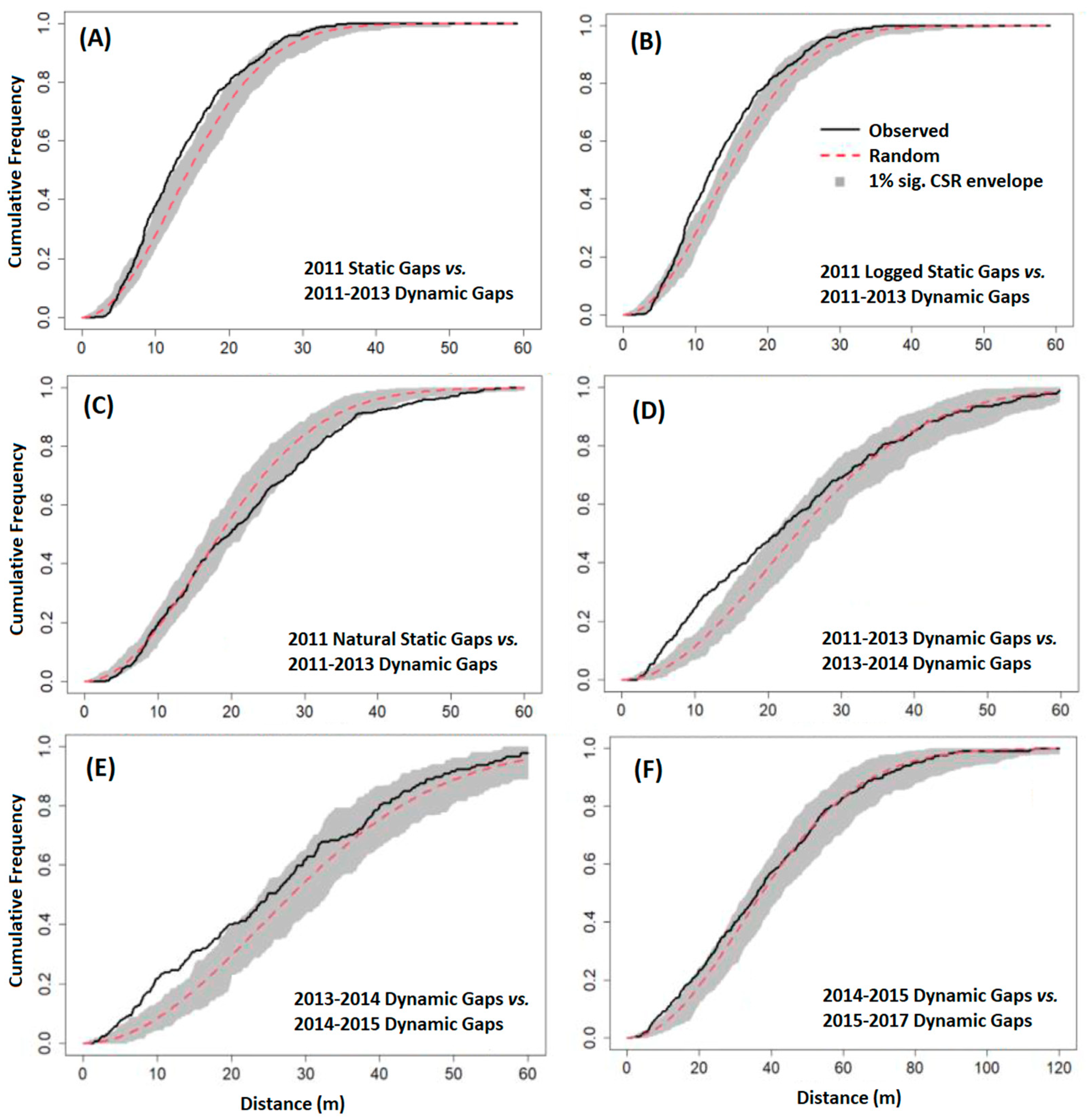
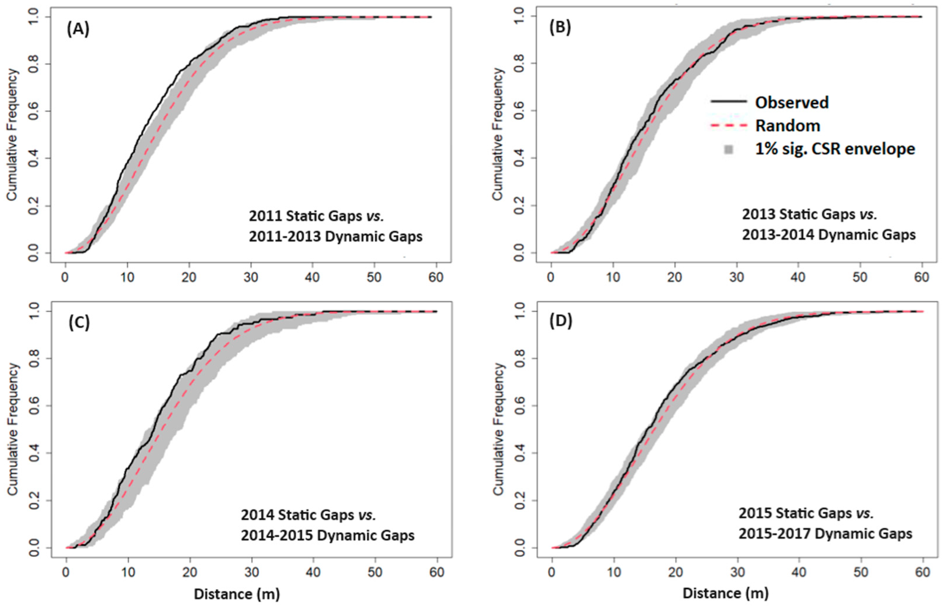
3.3. Gap Contagiousness

Figure 5 presents a series of graphs illustrating the spatial relationship between different types of gaps in a forested area over various time periods. Figure 5A demonstrates the cumulative distribution of nearest neighbor distances between all static gaps present in 2011 and the dynamic gaps created from 2011 to 2013. The solid black line represents the observed cumulative distribution, while the dashed lines delineate the complete spatial randomness (CSR) envelope, indicating the expected distribution under random conditions. If the observed line falls within the CSR envelope, it suggests no significant deviation from random spatial distribution. Conversely, if the observed line surpasses the CSR envelope, it indicates a clustered spatial relationship, implying gaps are closer together than random chance would predict. Figure 5B focuses specifically on static gaps resulting from logging activities in 2011, akin to Figure 5A’s setup. Figure 5C mirrors Figure 5A but concentrates on static gaps occurring naturally in 2011, excluding those attributed to logging. Figure 5D examines the spatial relationship between dynamic gaps from 2011 to 2013 and newly created dynamic gaps from 2013 to 2014, following the same interpretation guidelines as in Figure 5A–C. Figure 5E,F follow the pattern of Figure 5D, focusing on dynamic gaps created in subsequent periods and their spatial relationship with newly formed dynamic gaps. In general, each graph elucidates the spatial dependence of various gap types (static and dynamic) over distinct time spans. The solid black line represents observed spatial distributions, while the CSR envelope serves as a benchmark for random distribution.
Regarding the relationship between static and subsequent dynamic gaps (first experiment), we observed that only the static gaps from the 2011 period had a spatial relationship different from random (p < 0.01 at distances closer than 20 m) with the newly created dynamic gaps of the subsequent 2011–2013 period (Figure 5A). The nature of this relationship was clustered due to the cumulative distribution lying above the CSR envelope. The remaining static gaps visible in each time period did not differ from random with their subsequent dynamic gaps (Figure 6). When stratifying the static gaps between logged and natural gaps (second experiment), only the logged static gaps from 2011 showed a spatial relationship different from random and of clustered nature in relation to the dynamic gaps created in the subsequent period of 2011–2013 (p < 0.01 closer to 20 m of distance) (Figure 5B). The natural static gaps did not show a spatial relationship with newly created gaps different from random (p > 0.01) (Figure 5C). Finally, the comparison between dynamic gaps from one period with the subsequent periods (third experiment) showed a spatial relationship different from random between all analyzed time periods (p < 0.01 closer than 20 m) (Figure 5D–F). Therefore, all dynamic gaps (new gaps) affected the creation of new gaps up to 20 m of distance. This means that the gap contagious effect has a limited range around the gaps being created, where gaps may affect trees nearby to have a higher likelihood of felling, but not farther away than 20 m than the initial gaps.

4. Discussion

Using a time series of airborne LiDAR data, our research offers novel empirical insights into gap closure rates and identifies the associated modes of closure. Additionally, we examine human-induced gap contagion effects, attributing them to various gap types (static and dynamic) and their origins (natural or logging activities). This study highlights the potential uncertainties and overestimation of the structure of regenerating degraded forests and old-growth vegetation based on remote sensing observations of the top of canopy height. First, we show that gaps created by logging activities, distinct from naturally occurring ones, contribute to the formation of additional gaps. Consequently, gaps resulting from logging may exacerbate the further occurrence of mortality in forest ecosystems, thereby establishing a lasting legacy effect. While trees are adapted to average wind loads in their environment [41], the additional disturbances may be explained due to the opened gaps creating conditions for winds to unload [42,43,44]. Second, although the canopy gap quickly closes within a few years after the disturbance when looking from the top of the canopy, we show that the actual tree growth takes much longer, such as an average of seven years to close a gap (using 10 m as threshold) or 21 years to reach 30 m of height. Therefore, we highlight that remote sensing-based estimates of aboveground biomass or carbon of regenerating forests that only consider the top of the canopy height metric can potentially constitute an overestimate of the regenerating forest stand properties. Moreover, this recovery does not consider other factors such as the basal area and wood density of different species composition, which may increase even more the overestimate of recovery of these forests solely based on the top of the canopy height.
The mechanisms for closing the canopy gaps involve a combination of year-to-year lateral ingrowth and vertical growth with similar annual average rates of 16.7% yr−1. This means that lateral ingrowth was found to be a key process for the gap closure having a similar contribution compared to the vertical growth in this rainforest. The results may differ in other forests with distinct environmental and climatological conditions, which affect vertical growth rates. For example, a recent study observed a much lower relative contribution of the lateral gap closure (20%) compared to vertical (80%) over a longer period of time in a temperate forest [45], which is expected for a forest with a slower growth rate than a rainforest. Previous studies in dense tropical forests found similar but slightly higher values from 21 to 22% of annual rates of lateral ingrowth [26,46]. We estimated vertical growth for vegetation within gaps to a range between 1.3 and 1.7 m yr−1, values which are close to previous estimates of 1.6 m yr−1 in the same area [26]. However, in this study, the estimates were done per time interval to obtain more details on the variability of height growth. These values are within the range of growth rates of individuals from Cecropia sp. (1.2 to 1.5 m yr−1), one of the common pioneer tree species found in canopy gaps [47]. The height growth outside of gaps, and over nominally undisturbed canopies, was lower with an average of 0.7 m yr−1. We found that the number of static gaps in the forest remained stable over time, whereas the total area of all the gaps has a negative trend of steadily declining each year. Previous findings show that gaps created from logging events have a larger area than naturally occurring gaps [48,49]. This aligns with our empirical observations, i.e., large gap areas are prevalent right after logging, and as regeneration occurs, gaps close over time and split up into smaller gaps; thus, the number of gaps remains similar whereas the total combined area reduces.
The growth model that was fitted with the LiDAR data from multiple years allowed for the estimate of height growth based on the pre-existing height of vegetation as a predictor. This empirical data and established relationship, although showing weak strength (close to R2 = 0.15), allowed us to estimate the height growth of trees based on their current height and to estimate a period of six years for gaps to fully close (reach 10 m height), which comes close to what we observed empirically at the gap closure analysis. This model can contribute to the future development of estimates of carbon accumulation and the parametrization of ecosystem models leveraging remote sensing empirical data [50]. A common approach from previous studies involved aggregating aboveground biomass data from forests of different ages to build growth curves [51,52,53], a method called space-for-time substitution. There is a notable oversight concerning the intricate interplay between canopy gap dynamics and carbon dynamics, due to the rapid closure of gaps after disturbance potentially being perceived as a rapid increase in biomass as previously discussed. The use of repeated LiDAR data, alongside the methodology presented herein, holds promise in providing high-resolution empirical observations on height and height growth, thereby facilitating enhancements or validation of these space-for-time approaches in future studies. Examples of these approaches include quantifying the carbon accumulation in secondary forests using space-for-time substitution and a static biomass map from ESA/CCI [51,52,53]. The repeated LiDAR data and the approach we show here can contribute to providing high-resolution empirical observations on height and height growth to improve such approaches in the future. More repeated LiDAR data should be collected and analyzed over different environments to understand how they can affect these growth curves. Our analysis, however, does not come without limitations. LiDAR data have sources of error in vertical accuracy and geolocation, which affect the height-to-height growth relationships. In our analysis, the height growth of tall old-growth forests (>30 m) can be as low as a few centimeters, which is within the vertical error of ~0.15 m of the airborne LiDAR data.
Comparing height growth between the three different gap classes indicated no significant difference in vertical growth between logged and natural gaps. This supports previous findings showing statistically similar rates of recovery between different types and intensities of disturbance in tropical forests [54]. Previous findings showed that heavily logged forests experience faster growth rates than undisturbed forests [55]. This was not the case with our study area, which had low logging intensity (2 trees ha−1 and 16.3 m3 ha−1). When comparing growth within gaps to the undisturbed canopy, the data collected followed the expected pattern of lower starting vegetation located within gaps having greater annual growth than the taller non-gapped canopy. The gapped locations showed a significant increase in growth for all years when compared to nominally undisturbed canopy cover, as expected due to the fast growth and colonization of pioneer species [49,56]. In our study area, trees inside gaps grew on average 2.2 times faster (1.5 m yr−1) than trees at the surrounding canopy (0.7 m yr−1) closing gaps over time.
Our findings partially supported the spatial contagiousness of disturbance hypothesis (gap contagiousness). We show that this effect is dependent on gap type, meaning only recently created gaps were positively associated with the creation of new gaps (dynamic vs. dynamic gaps). This supports a legacy effect of logging causing increased tree damage even after six years post-disturbance. However, overall, the findings did not support the hypothesis when considering pre-existing gaps (static) versus new gaps (dynamic). An exception can be made when considering the origin of gaps. Recently opened gaps in 2011 due to logging activities showed a small but significant (p < 0.01 in 10–20 m distance) signal of spatial dependence with newly created gaps. Newly created gaps are more likely to cause gaps to be located nearby (<20 m of distance), with this most likely being related to tree damage (e.g., branch or crown fall) or mortality due to snapping or uprooting [57]. This further explains the absence of any spatial pattern when comparing static gaps, as the static definition includes all gaps below the threshold, including older gaps and those that may not represent mortality. This finding also supports the understanding that not all gaps are connected to mortality [13,16]. Compared to previous studies, we expect that the analysis of Jansen et al. (2008) [29] did not confirm any spatial dependence between gaps, because they were looking at all the gaps within the forest, whereas our study was able to stratify and attribute gaps to different types (static or dynamic) and origins (natural or logging). A previous study suggests the increased treefall rates in logged forests related to canopy openings [58]. This in part corroborates with our findings explaining why logged static gaps from 2011 showed contagiousness with newly created gaps. This phenomenon should still be tested in other regions to bring more evidence of its occurrence and further tests are required to determine the magnitude of the potential increased mortality after logging.
The results presented here have implications for the understanding of the impacts of forest degradation due to logging in tropical forests. Through the time series of LiDAR remote sensing observations, we show that gaps close very fast in a matter of two to seven years and the ones associated with felled trees may induce the occurrence of other gap openings associated with tree damage or mortality until six years post-disturbance. Through this increase in tree mortality post-logging, our findings support that logging can be the driver of forest degradation in the Brazilian Amazon forests, contributing to carbon emissions [6,59,60,61]. The magnitude of this increase in mortality remains to be tested in future studies. It remains an open question as to whether the doubled rate of regeneration of vegetation inside gaps, in comparison to non-gaps, can offset the losses in carbon (of felled trees and legacy effects); this is beyond the scope of this paper but is an important question to be answered regarding the fate of logged forests of the Brazilian Amazon. We further suggest that the observation of these regenerating degraded forests using remote sensing techniques should be made with caution. Overestimating the structure and carbon stocks in degraded forests can occur when considering only the top of the canopy height because of the quick occlusion of gaps by lateral ingrowth after disturbance. Alternative methods considering metrics that also look beneath the top of the canopy and inside the understory should be considered. The approach applied here has the potential to extract empirical data to help improve the understanding of regenerating forests and to be used for better parametrization of ecosystem models that explicitly consider gap-phase dynamics.

5. Conclusions

The process by which gaps open and close was investigated using a time series of airborne LiDAR data in the Brazilian Amazon’s Jamari National Forest. Lateral ingrowth was found to be a key process for gap closure having a similar contribution compared to vertical growth when consolidated over time. Closing gaps at an average of 16.7% of gap area per year, our growth model indicated that it might take up to seven years on average to close a gap (10 m of height) solely through vertical growth. There was no significant difference between natural and logged gaps in terms of mean growth. However, vegetation inside gaps grew significantly faster than the surrounding undisturbed canopy.
Our study extends the understanding of the spatial contagiousness of disturbances supporting the hypothesis for certain gap types and origins. Newly created gaps tend to be clustered around older logged static gaps, but not necessarily with natural static gaps. This fact suggests a legacy effect of the logging activities on the dynamics of these forests, characterized by boosted post-logging mortality. Further evidence of gap contagion was only found between sets of dynamic gaps in different time periods, which reinforces the idea that gap contagion is related to tree mortality as opposed to the presence of any gap that might not be related to mortality.
This study demonstrated the use of multi-temporal airborne LiDAR for monitoring changes in the canopy after logging activities. The approach proposed here was particularly beneficial for mapping growth within the gaps, something that would not be possible without using multitemporal LiDAR observations. Further research venues should look at the growth models, using them to calculate aboveground biomass and estimate carbon, specifically measuring how gap closure modes (lateral and vertical) affect carbon balance in an ecosystem model.

Supplementary Materials

The following supporting information can be downloaded at: https://www.mdpi.com/article/10.3390/rs16132319/s1, Figure S1: Height growth (m yr−1) estimated between LiDAR acquisitions over gaps classed as logged or natural, and over non-gap locations, Table S1: Summary of vertical height growth within dynamic gaps between each LiDAR acquisition.

Author Contributions

Conceptualization, P.W., R.D. and P.d.C.B.; methodology, P.W., R.D. and P.d.C.B.; software, P.W.; validation, P.W.; formal analysis, P.W. and R.D.; investigation, P.W. and R.D.; resources, R.D. and P.d.C.B.; data curation, P.W.; writing—original draft preparation, P.W. and S.M.; writing—review and editing, S.M., D.B., R.D., L.S.G. and P.d.C.B.; visualization, P.W.; supervision, R.D. and P.d.C.B. All authors have read and agreed to the published version of the manuscript.

Funding

P.d.C.B. thanks the SEED University of Manchester for the Personal Research and Scholarship Allowances (PRSA), which supported and facilitated the support research efforts.

Data Availability Statement

Data and codes can be found at https://zenodo.org/record/5337079#.YS0vaYjdtPY (accessed on 10 August 2023).

Acknowledgments

We thank the Brazilian Forest Service, the Sustainable Landscapes Brazil project supported by the Brazilian Agricultural Research Corporation (EMBRAPA), the US Forest Service, USAID, and the US Department of State, for providing the airborne LiDAR data and the forest inventory.

Conflicts of Interest

Author Ricardo Dalagnol was employed by the company CTrees. The remaining authors declare that the research was conducted in the absence of any commercial or financial relationships that could be construed as a potential conflict of interest.

References

  1. ter Steege, H.; Pitman, N.C.A.; Sabatier, D.; Baraloto, C.; Salomao, R.P.; Guevara, J.E.; Phillips, O.L.; Castilho, C.V.; Magnusson, W.E.; Molino, J.-F.; et al. Hyperdominance in the Amazonian Tree Flora. Science 2013, 342, 1243092. [Google Scholar] [CrossRef] [PubMed]
  2. Pan, Y.; Birdsey, R.A.; Fang, J.; Houghton, R.; Kauppi, P.E.; Kurz, W.A.; Phillips, O.L.; Shvidenko, A.; Lewis, S.L.; Canadell, J.G.; et al. A large and persistent carbon sink in the world’s forests. Science 2011, 333, 988–993. [Google Scholar] [CrossRef] [PubMed]
  3. Gatti, L.V.; Basso, L.S.; Miller, J.B.; Gloor, M.; Gatti Domingues, L.; Cassol, H.L.G.; Tejada, G.; Aragão, L.E.O.C.; Nobre, C.; Peters, W.; et al. Amazonia as a carbon source linked to deforestation and climate change. Nature 2021, 595, 388–393. [Google Scholar] [CrossRef] [PubMed]
  4. Lapola, D.M.; Pinho, P.; Barlow, J.; Aragão, L.E.O.C.; Berenguer, E.; Carmenta, R.; Liddy, H.M.; Seixas, H.; Silva, C.V.J.; Silva-Junior, C.H.L.; et al. The Drivers and Impacts of Amazon Forest Degradation. Science 2023, 379, 349. [Google Scholar] [CrossRef]
  5. Silva Junior, C.H.L.; Aragão, L.E.O.C.; Anderson, L.O.; Fonseca, M.G.; Shimabukuro, Y.E.; Vancutsem, C.; Achard, F.; Beuchle, R.; Numata, I.; Silva, C.A.; et al. Persistent collapse of biomass in Amazonian forest edges following deforestation leads to unaccounted carbon losses. Sci. Adv. 2020, 6, eaaz8360. [Google Scholar] [CrossRef] [PubMed]
  6. Matricardi, E.A.T.; Skole, D.L.; Costa, O.B.; Pedlowski, M.A.; Samek, J.H.; Miguel, E.P. Long-term forest degradation surpasses deforestation in the Brazilian Amazon. Science 2020, 369, 1378–1382. [Google Scholar] [CrossRef] [PubMed]
  7. Broadbent, E.N.; Asner, G.P.; Keller, M.; Knapp, D.E.; Oliveira, P.J.; Silva, J.N. Forest fragmentation and edge effects from deforestation and selective logging in the Brazilian Amazon. Biol. Conserv. 2008, 141, 1745–1757. [Google Scholar] [CrossRef]
  8. Yamamoto, S.-I. Forest Gap Dynamics and Tree Regeneration. J. For. Res. 2000, 5, 223–229. [Google Scholar] [CrossRef]
  9. Brokaw, N.V.L. The Definition of Treefall Gap and Its Effect on Measures of Forest Dynamics. Biotropica 1982, 14, 158–160. [Google Scholar] [CrossRef]
  10. Negrón-Juárez, R.I.; Chambers, J.Q.; Marra, D.M.; Ribeiro, G.H.P.M.; Rifai, S.W.; Higuchi, N.; Roberts, D. Detection of Subpixel Treefall Gaps with Landsat Imagery in Central Amazon Forests. Remote Sens. Environ. 2011, 115, 3322–3328. [Google Scholar] [CrossRef]
  11. Gora, E.M.; Burchfield, J.C.; Muller-Landau, H.C.; Bitzer, P.M.; Yanoviak, S.P. Pantropical Geography of Lightning-Caused Disturbance and Its Implications for Tropical Forests. Glob. Chang. Biol. 2020, 26, 5017–5026. [Google Scholar] [CrossRef] [PubMed]
  12. Dalagnol, R.; Wagner, F.H.; Galvão, L.S.; Streher, A.S.; Phillips, O.L.; Gloor, E.; Pugh, T.A.M.; Ometto, J.P.H.B.; Aragão, L.E.O.C. Large-scale variations in the dynamics of Amazon forest canopy gaps from airborne lidar data and opportunities for tree mortality estimates. Sci. Rep. 2021, 11, 1388. [Google Scholar] [CrossRef] [PubMed]
  13. Brokaw, N.V.L. Gap-Phase Regeneration in a Tropical Forest. Ecology 1985, 66, 682–687. [Google Scholar] [CrossRef]
  14. Schnitzer, S.A.; Carson, W.P. Treefall Gaps and the Maintenance of Species Diversity in a Tropical Forest. Ecology 2001, 82, 913–919. [Google Scholar] [CrossRef]
  15. Hartshorn, G. Tree falls and tropical forest dynamics Book reviews View project Tropical forest vegetation descriptions View project. In Tropical Trees as Living Systems; Cambridge University Press: Cambridge, UK, 1978; pp. 617–638. [Google Scholar]
  16. Espírito-Santo, F.D.B.; Keller, M.M.; Linder, E.; Oliveira Junior, R.C.; Pereira, C.; Oliveira, C.G. Gap formation and carbon cycling in the Brazilian Amazon: Measurement using high-resolution optical remote sensing and studies in large forest plots. Plant Ecol. Divers. 2013, 7, 305–318. [Google Scholar] [CrossRef]
  17. Hunter, M.O.; Keller, M.; Morton, D.; Cook, B.; Lefsky, M.; Ducey, M.; Saleska, S.; de Oliveira, R.C.; Schietti, J. Structural Dynamics of Tropical Moist Forest Gaps. PLoS ONE 2015, 10, e0132144. [Google Scholar] [CrossRef] [PubMed]
  18. Zhang, K. Identification of gaps in mangrove forests with airborne LIDAR. Remote Sens. Environ. 2008, 112, 2309–2325. [Google Scholar] [CrossRef]
  19. Almeida, D.R.A.; Broadbent, E.N.; Zambrano, A.M.A.; Wilkinson, B.E.; Ferreira, M.E.; Chazdon, R.; Meli, P.; Gorgens, E.B.; Silva, C.A.; Stark, S.C.; et al. Monitoring the structure of forest restoration plantations with a drone-lidar system. Int. J. Appl. Earth Obs. Geoinf. 2019, 79, 192–198. [Google Scholar] [CrossRef]
  20. Almeida, D.R.A.; Stark, S.C.; Chazdon, R.; Nelson, B.W.; Cesar, R.G.; Meli, P.; Gorgens, E.B.; Duarte, M.M.; Valbuena, R.; Moreno, V.S.; et al. The effectiveness of lidar remote sensing for monitoring forest cover attributes and landscape restoration. For. Ecol. Manag. 2019, 438, 34–43. [Google Scholar] [CrossRef]
  21. Jucker, T. Deciphering the Fingerprint of Disturbance on the Three-Dimensional Structure of the World’s Forests. New Phytol. 2022, 233, 612–617. [Google Scholar] [CrossRef] [PubMed]
  22. Koukoulas, S.; Blackburn, G.A. Quantifying the spatial properties of forest canopy gaps using LiDAR imagery and GIS. Int. J. Remote Sens. 2004, 25, 3049–3072. [Google Scholar] [CrossRef]
  23. Espírito-Santo, F.D.B.; Gloor, M.; Keller, M.; Malhi, Y.; Saatchi, S.; Nelson, B.; Junior, R.C.O.; Pereira, C.; Lloyd, J.; Frolking, S.; et al. Size and frequency of natural forest disturbances and the Amazon forest carbon balance. Nat. Commun. 2014, 5, 3434. [Google Scholar] [CrossRef] [PubMed]
  24. Gaulton, R.; Malthus, T.J. LiDAR mapping of canopy gaps in continuous cover forests: A comparison of canopy height model and point cloud based techniques. Int. J. Remote Sens. 2010, 31, 1193–1211. [Google Scholar] [CrossRef]
  25. Leitold, V.; Morton, D.C.; Longo, M.; dos-Santos, M.N.; Keller, M.; Scaranello, M. El Niño drought increased canopy turnover in Amazon forests. New Phytol. 2018, 219, 959–971. [Google Scholar] [CrossRef] [PubMed]
  26. Dalagnol, R.; Phillips, O.L.; Gloor, E.; Galvão, L.S.; Wagner, F.H.; Locks, C.J.; Aragão, L.E.O.C. Quantifying Canopy Tree Loss and Gap Recovery in Tropical Forests under Low-Intensity Logging Using VHR Satellite Imagery and Airborne LiDAR. Remote Sens. 2019, 11, 817. [Google Scholar] [CrossRef]
  27. Asner, G.P.; Keller, M.; Silva, J.N.M. Spatial and temporal dynamics of forest canopy gaps following selective logging in the eastern Amazon. Glob. Chang. Biol. 2004, 10, 765–783. [Google Scholar] [CrossRef]
  28. Vaughn, N.R.; Asner, G.P.; Giardina, C.P. Long-term fragmentation effects on the distribution and dynamics of canopy gaps in a tropical montane forest. Ecosphere 2015, 6, art271. [Google Scholar] [CrossRef]
  29. Jansen, P.A.; Meer, P.J.V.; der Bongers, F. Spatial Contagiousness of Canopy Disturbance in Tropical Rain Forest: An Individual-Tree-Based Test. Ecology 2008, 89, 3490–3502. [Google Scholar] [CrossRef] [PubMed]
  30. Vepakomma, U.; St-Onge, B.; Kneeshaw, D. Spatially Explicit Characterization of Boreal Forest Gap Dynamics Using Multi-Temporal Lidar Data. Remote Sens. Environ. 2008, 112, 2326–2340. [Google Scholar] [CrossRef]
  31. Pryke, J.S.; Samways, M.J. Conservation management of complex natural forest and plantation edge effects. Landsc. Ecol. 2011, 27, 73–85. [Google Scholar] [CrossRef]
  32. Lenz, B.B.; Jack, K.M.; Spironello, W.R. Edge effects in the primate community of the biological dynamics of forest fragments project, Amazonas, Brazil. Am. J. Phys. Anthropol. 2014, 155, 436–446. [Google Scholar] [CrossRef] [PubMed]
  33. Cysneiros, V.C.; Machado, S.d.A.; Pelissari, A.L.; Figueiredo Filho, A.; Urbano, E. Modeling of the Commercial Volume Stock in an Ombrophilous Forest in the Southwest of the Amazon. Cerne 2016, 22, 457–464. [Google Scholar] [CrossRef]
  34. ICMBio Plano de Manejo da Floresta Nacional do Jamari; Diagnóstico: Brasília, Brazil, 2005.
  35. Leitold, V.; Keller, M.; Morton, D.C.; Cook, B.D.; Shimabukuro, Y.E. Airborne lidar-based estimates of tropical forest structure in complex terrain: Opportunities and trade-offs for REDD+. Carbon Balance and Management 2015, 10, 3. [Google Scholar] [CrossRef] [PubMed]
  36. Isenburg, M. GitHub—Kheaactua/LAStools: Efficient Tools for LiDAR Processing. GitHub, 2015. Available online: https://github.com/kheaactua/LAStools#readme (accessed on 27 July 2021).
  37. Jean-Romain. GitHub—Jean-Romain/lidR: R Package for Airborne LiDAR Data Manipulation and Visualisation for Forestry Application. GitHub, 2021. Available online: https://github.com/Jean-Romain/lidR (accessed on 27 July 2021).
  38. R Core Team. R: A Language and Environment for Statistical ## Computing; R Foundation for Statistical Computing: Vienna, Austria, 2021; Available online: https://www.R-project.org/ (accessed on 3 February 2021).
  39. Baddeley, A.; Ruban, E.; Turner, R. Spatial Point Patterns: Methodology and Applications with R; Routledge & CRC Press: London, UK, 2015; Available online: https://www.routledge.com/Spatial-Point-Patterns-Methodology-and-Applications-with-R/Baddeley-Rubak-Turner/9781482210200/ (accessed on 24 August 2021).
  40. Baddeley, A.; Turner, R.; Rubak, E. Spatstat—Spatstat Website. Spatstat.org, 2014. Available online: https://spatstat.org/ (accessed on 27 July 2021).
  41. Bonnesoeur, V.; Constant, T.; Moulia, B.; Fournier, M. Forest trees filter chronic wind-signals to acclimate to high winds. New Phytol. 2016, 210, 850–860. [Google Scholar] [CrossRef] [PubMed]
  42. Mitchell, A.R.; Tapley, I.; Milne, A.; Williams, M.L.; Zhou, Z.; Lehmann, E.; Caccetta, P.; Lowell, K.; Held, A. C- and L-band SAR interoperability: Filling the gaps in continuous forest cover mapping in Tasmania. Remote Sens. Environ. 2014, 155, 58–68. [Google Scholar] [CrossRef]
  43. Aleixo, I.; Norris, D.; Hemerik, L.; Barbosa, A.; Prata, E.; Costa, F.; Poorter, L. Amazonian rainforest tree mortality driven by climate and functional traits. Nat. Clim. Change 2019, 9, 384–388. [Google Scholar] [CrossRef]
  44. Kamimura, B.A.; Magnani, M.; Luciano, W.A.; Campagnollo, F.B.; Pimentel, T.C.; Alvarenga, V.O.; Pelegrino, B.O.; Cruz, A.G. Brazilian Artisanal Cheeses: An Overview of their Characteristics, Main Types and Regulatory Aspects. Compr. Rev. Food Sci. Food Saf. 2019, 18, 1636–1657. [Google Scholar] [CrossRef] [PubMed]
  45. Vepakomma, U.; St-Onge, B.; Kneeshaw, D. Response of a boreal forest to canopy opening: Assessing vertical and lateral tree growth with multi-temporal lidar data. Ecol. Appl. 2011, 21, 99–121. [Google Scholar] [CrossRef] [PubMed]
  46. Clark, D.A.; Clark, D.B. Getting to the Canopy: Tree Height Growth in a Neotropical Rain Forest. Ecology 2001, 82, 1460–1472. [Google Scholar] [CrossRef]
  47. Krüger, K.; Send, C.; Jucker, T.; Pflugmacher, D.; Seidl, R. Gap Expansion Is the Dominant Driver of Canopy Openings in a Temperate Mountain Forest Landscape. J. Ecol. 2024, 1365–2745, 14320. [Google Scholar] [CrossRef]
  48. Kent, R.; Lindsell, J.; Laurin, G.; Valentini, R.; Coomes, D. Airborne LiDAR Detects Selectively Logged Tropical Forest Even in an Advanced Stage of Recovery. Remote Sens. 2015, 7, 8348–8367. [Google Scholar] [CrossRef]
  49. Felton, A.; Felton, A.M.; Wood, J.; Lindenmayer, D.B. Vegetation structure, phenology, and regeneration in the natural and anthropogenic tree-fall gaps of a reduced-impact logged subtropical Bolivian forest. For. Ecol. Manag. 2006, 235, 186–193. [Google Scholar] [CrossRef]
  50. Génin, A.; Majumder, S.; Sankaran, S.; Danet, A.; Guttal, V.; Schneider, F.D.; Kéfi, S. Monitoring ecosystem degradation using spatial data and the R package spatial warnings. Methods Ecol. Evol. 2018, 9, 2067–2075. [Google Scholar] [CrossRef]
  51. Heinrich, V.H.A.; Dalagnol, R.; Cassol, H.L.G.; Rosan, T.M.; de Almeida, C.T.; Silva Junior, C.H.L.; Campanharo, W.A.; House, J.I.; Sitch, S.; Hales, T.C.; et al. Large Carbon Sink Potential of Secondary Forests in the Brazilian Amazon to Mitigate Climate Change. Nat. Commun. 2021, 12, 1785. [Google Scholar] [CrossRef] [PubMed]
  52. Heinrich, V.H.A.; Vancutsem, C.; Dalagnol, R.; Rosan, T.M.; Fawcett, D.; Silva-Junior, C.H.L.; Cassol, H.L.G.; Achard, F.; Jucker, T.; Silva, C.A.; et al. The Carbon Sink of Secondary and Degraded Humid Tropical Forests. Nature 2023, 615, 436–442. [Google Scholar] [CrossRef] [PubMed]
  53. Fawcett, D.; Sitch, S.; Ciais, P.; Wigneron, J.P.; Silva-Junior, C.H.L.; Heinrich, V.; Vancutsem, C.; Achard, F.; Bastos, A.; Yang, H.; et al. Declining Amazon Biomass due to Deforestation and Subsequent Degradation Losses Exceeding Gains. Glob. Chang. Biol. 2023, 29, 1106–1118. [Google Scholar] [CrossRef] [PubMed]
  54. Rappaport, D.I.; Morton, D.C.; Longo, M.; Keller, M.; Dubayah, R.; Dos-Santos, M.N. Quantifying long-term changes in carbon stocks and forest structure from Amazon forest degradation. Environ. Res. Lett. 2018, 13, 065013. [Google Scholar] [CrossRef]
  55. Chapman, C.A.; Chapman, L.J. Forest regeneration in logged and unlogged forests of Kibale National Park, Uganda. Biotropica 1997, 29, 396–412. [Google Scholar] [CrossRef]
  56. Kyei, E.; Bondzie-Mensah, M. Effect of Canopy Gaps on Composition and Diversity of Natural Regeneration Following Selective Logging in a Moist Evergreen Forest in Ghana; ResearchGate: Berlin, Germany, 2020; Available online: https://www.researchgate.net/publication/339428624_Effect_of_canopy_gaps_on_composition_and_diversity_of_natural_regeneration_following_selective_logging_in_a_moist_evergreen_forest_in_Ghana/link/5ebea607299bf1c09abc9381/download (accessed on 11 August 2021).
  57. Arellano, G.; Medina, N.G.; Tan, S.; Mohamad, M.; Davies, S.J. Crown Damage and the Mortality of Tropical Trees. New Phytol. 2019, 221, 169–179. [Google Scholar] [CrossRef] [PubMed]
  58. Schulze, M.; Zweede, J. Canopy dynamics in unlogged and logged forest stands in the eastern Amazon. For. Ecol. Manag. 2006, 236, 56–64. [Google Scholar] [CrossRef]
  59. de Moura, Y.M.; Balzter, H.; Galvão, L.S.; Dalagnol, R.; Espírito-Santo, F.; Santos, E.G.; Garcia, M.; Bispo, P.d.C.; Oliveira, R.C.; Shimabukuro, Y.E. Carbon Dynamics in a Human-Modified Tropical Forest: A Case Study Using Multi-Temporal LiDAR Data. Remote Sens. 2020, 12, 430. [Google Scholar] [CrossRef]
  60. Dalagnol, R.; Wagner, F.H.; Galvão, L.S.; Braga, D.; Osborn, F.; Sagang, L.B.; Da Conceição Bispo, P.; Payne, M.; Silva Junior, C.; Favrichon, S.; et al. Mapping Tropical Forest Degradation with Deep Learning and Planet NICFI Data. Remote Sens. Environ. 2023, 298, 113798. [Google Scholar] [CrossRef]
  61. Mills, M.; Malhi, Y.; Ewers, R.M.; Kho, L.K.; Teh, Y.A.; Both, S.; Burslem, D.F.R.P.; Majalap, N.; Nilus, R.; Huasco, W.H.; et al. Tropical forests post-logging are a persistent net carbon source to the atmosphere. Proc. Natl. Acad. Sci. USA 2023, 120, e2214462120. [Google Scholar] [CrossRef] [PubMed]
Figure 1. The location of the study area in Jamari National Forest, Rondônia, Brazil. The left panel shows the canopy height model acquired in 2011 in the background and the location of logged trees.
Remotesensing 16 02319 g001
Figure 2. Dynamic gaps delineated within the study area between all four periods of LiDAR acquisitions. The background image corresponds to a very high-resolution image from Google Satellite basemaps.
Remotesensing 16 02319 g002
Figure 3. Visual representation of the gap closure process dominated by lateral ingrowth over time within an example gap of the study area. The left and bottom panels show a summary of all the ingrowth laid on top of the original 2011 gap outline. Each color band represents the time interval between LiDAR data acquisitions that partially closed the gap.
Remotesensing 16 02319 g003
Figure 4. Relationship between height (m) and height gain (m year−1) calculated from a 10,000-sample composed of 2,356,872 pixels of 1 m2, showing positive changes in the CHM between LiDAR acquisitions. The red line indicates an exponential model showing the predicted values for height gain based on the original height. The blue outline represents a 95% confidence level.
Remotesensing 16 02319 g004
Figure 5. Gaps and their spatial dependence on pre-existing gaps. Cumulative distribution of nearest neighbor distances alongside a complete spatial randomness (CSR) envelope of 1% significance for (A) all static gaps of 2011 and newly created dynamic gaps for 2011–2013; (B) logged static gaps of 2011 and newly created dynamic gaps for 2011–2013; (C) natural static gaps of 2011 and newly created dynamic gaps for 2011–2013; (D) dynamic gaps created between 2011 and 2013 and newly created dynamic gaps between 2013 and 2014; (E) dynamic gaps created between 2013 and 2014 and newly created dynamic gaps between 2014 and 2015; and (F) dynamic gaps created between 2014 and 2015 and newly created dynamic gaps between 2015 and 2017. When the observed solid line in black falls within the CSR envelope, the spatial relationship is not different from random at a 1% significance level. In contrast, when the observed line lies above the CSR, the nature of the spatial relationship is clustered.
Remotesensing 16 02319 g005
Figure 6. Dynamic gaps (new gaps) of each time period and their spatial dependence on static gaps visible in the previous time period. Cumulative distribution of nearest neighbor distances alongside a complete spatial randomness (CSR) envelope of 1% significance for (A) all static gaps of 2011 and newly created dynamic gaps for 2011–2013; (B) all static gaps of 2013 and newly created dynamic gaps for 2013–2014; (C) all static gaps of 2014 and newly created dynamic gaps for 2014–2015; (D) all static gaps of 2015 and newly created dynamic gaps for 2015–2017. When the observed solid line in black falls within the CSR envelope, the spatial relationship is not different from random at a 1% significance level. In contrast, when the observed line lies above the CSR, the nature of the spatial relationship is clustered.
Remotesensing 16 02319 g006
Table 1. Summary of acquisition information regarding the airborne LiDAR point clouds that were collected in UPA-01 between 2011 and 2017. The point cloud density unit in ppm2 consists of points per square meter.
Information20112013201420152017
Laser Scan Sensor Optech 3100Optech, OrionTrimble, Harrier 68iOptech 3100Optech ALTM Gemini
Acquisition date 17 November 201120 September 201310 September 201421 September 201520 April 2017
Acquisition altitude (m)850853500750700
Off-nadir angle (°)11.111.1151515
Scan frequency (kHz)59.867.5400100100
Average point cloud density (ppm2)15.415.530.433.612
Table 2. Summary of the gap contagiousness experiments and the datasets compared with spatial analyses.
First Spatial DatasetSecond Spatial Dataset
Experiment 1—Static gaps vs. subsequent dynamic gaps:
2011 Static Gaps 2011–2013 Dynamic Gaps
2013 Static Gaps 2013–2014 Dynamic Gaps
2014 Static Gaps2014–2015 Dynamic Gaps
2015 Static Gaps2015–2017 Dynamic Gaps
Experiment 2—Static gaps from 2011 stratified by type vs. subsequent dynamic gaps:
2011 Logged Gaps 2011–2013 Dynamic Gaps
2011 Natural Gaps 2011–2013 Dynamic Gaps
Experiment 3—Dynamic gaps vs. subsequent dynamic gaps:
2011–2013 Dynamic Gaps 2013–2014 Dynamic Gaps
2013–2014 Dynamic Gaps 2014–2015 Dynamic Gaps
2014–2015 Dynamic Gaps 2015–2017 Dynamic Gaps
Table 3. The number of static gaps and their total area for each LiDAR acquisition date between 2011 and 2017.
YearArea (m2)Number of Static GapsMean Gap Area (m2)Gap Fraction (%)
201183,806115672.58.4
201356,563106952.95.6
201456,366107452.55.6
201543,13893945.94.3
201743,908101743.24.4
Table 4. Dynamic gap openings and closures over time for LiDAR data acquisition intervals. Values were normalized to average gaps per year.
Newly Open Dynamic Gaps
(Gaps per Year)
Closed Dynamic Gaps
(Gaps per Year)
2011–2013230.1212.5
2013–2014306.7260.0
2014–2015191.8321.5
2015–2017352.4200.9
Table 5. The total area of static gaps from 2011 (m2) that remained open or were completely closed (reaching a 10 m height gap threshold) in each year after logging.
YearGap Closed Vertically (m2)Gaps Closed Laterally (m2)Gaps Remain Open (m2)
201313,06121,58348,664
20148754692232,988
20157365391721,706
20176770449310,443
Sum35,95036,915-
Disclaimer/Publisher’s Note: The statements, opinions and data contained in all publications are solely those of the individual author(s) and contributor(s) and not of MDPI and/or the editor(s). MDPI and/or the editor(s) disclaim responsibility for any injury to people or property resulting from any ideas, methods, instructions or products referred to in the content.

