Abstract
With the development of hyperspectral sensors, the availability of hyperspectral images (HSIs) has increased significantly, prompting advancements in deep learning-based hyperspectral image classification (HSIC) methods. Recently, graph convolutional networks (GCNs) have been proposed to process graph-structured data in non-Euclidean domains, and have been used for HSIC. The superpixel segmentation should be implemented first in the GCN-based methods, however, it is difficult to manually select the optimal superpixel segmentation sizes to obtain the useful information for classification. To solve this problem, we constructed a HSIC model based on a multiscale feature search-based graph convolutional network (MFSGCN) in this study. Firstly, pixel-level features of HSIs are extracted sequentially using 3D asymmetric decomposition convolution and 2D convolution. Then, superpixel-level features at different scales are extracted using multilayer GCNs. Finally, the neural architecture search (NAS) method is used to automatically assign different weights to different scales of superpixel features. Thus, a more discriminative feature map is obtained for classification. Compared with other GCN-based networks, the MFSGCN network can automatically capture features and obtain higher classification accuracy. The proposed MFSGCN model was implemented on three commonly used HSI datasets and compared to some state-of-the-art methods. The results confirm that MFSGCN effectively improves accuracy.
1. Introduction
The advancement of hyperspectral imaging technology allows hyperspectral images (HSIs) to have higher spectral resolution in continuous narrow bands and better spatial characteristics of objects [1]. Leveraging the rich spectral and spatial information inherent in hyperspectral images facilitates detailed analysis of object type, composition, and distribution at the image elemental level. Hyperspectral image classification (HSIC) is a hot research problem in the field of image processing, focusing on the identification and classification of features based on their reflectance values in the spectral domain and their spatial relationships with neighboring features [2]. It identifies and classifies features based on the reflectance values reflected by the features in the spectral dimension and the neighborhood relationships between neighboring features in the spatial dimension. The ultimate goal of classification is to assign a unique class identity to each image element in the image. HSIC, as the basis of remote sensing image processing tasks, has been widely used in precision agriculture [3], geological exploration [4], environmental monitoring [5], medical diagnosis [6], and other fields.
The traditional remote sensing image classification method mainly analyzes and selects the spatial and spectral information of each type of feature contained within the remote sensing image. Then, each image element in the image is classified into a corresponding category according to a specific classification rule to achieve the purpose of image classification. However, a single criterion often fails to effectively distinguish between feature types with similar spectra. These approaches typically rely on shallow feature extraction through manual methods, limiting their ability to process large-scale remote sensing images efficiently, especially those comprising megabytes of data or more. In recent years, deep learning-based HSIC methods have sprung up. Advanced neural network models excel in extracting deeper, more representative image features capable of distinguishing diverse feature classes. Deep learning originates from the study of neural networks. Inspired by neuroscience research on the human brain, artificial neural networks (ANNs) were proposed to simulate the human brain to process data. By learning inherent patterns and hierarchical representations from sample data, deep learning demonstrates robust capabilities in recognizing various types of information such as text, images, and sounds. The concept of deep learning was first introduced to HSIC in 2014, when Chen et al. used an unsupervised learning-based self-encoder method to extract depth features from hyperspectral images [7]. Since then, more and more deep neural network models have been applied to HSIC. These methods are able to process large-scale data faster and can achieve higher classification accuracy based on few training samples. They show great advantages in classification tasks and have become a hot research topic.
Since deep learning algorithms can extract strong representational deep features from data in a hierarchical manner without manual selection, they received a lot of recognition and further research after being introduced into the hyperspectral field. Several common deep learning algorithms for HSIC include stacked autoencoders (SAEs) [8], deep belief networks (DBNs) [9], recurrent neural networks (RNNs) [10], convolutional neural networks (CNNs) [11,12], generative adversarial networks (GANs) [13], and graph convolutional networks (GCNs) [14]. These methods excel in extracting adaptive shallow and deep features, demonstrating strong recognition abilities in complex scenarios. State-of-the-art models efficiently incorporate both spectral and spatial information, leveraging deep and shallow image features to achieve exceptionally high classification accuracy in minimal time. The computational demand scales with the complexity of the network structure, influenced by the types, levels, and functional modules employed, which are critical factors affecting classification accuracy.
GCNs have been applied to HSIC due to their ability to handle irregular topological data, overcoming the limitation that convolutional neural networks can only handle Euclidean data (e.g., grid data). Although CNNs have powerful feature extraction capability and show great advantages in hyperspectral image classification, they can only extract spectral and spatial features of regular regions in the neighborhood of target pixels and cannot adapt to irregular feature distribution features. By converting conventional hyperspectral datasets into graph-structured data comprising nodes and edges, GCNs process the entire image directly, enabling learning of long-range relational features. Applying GCNs in hyperspectral image classification not only facilitates extraction of multiscale features and enhances classification accuracy, but also reduces computational complexity and shortens training times. Specifically, GCNs can treat the pixels in an image as nodes, map the whole image appropriately into a new discriminative space, and discriminate the attribute features of the pixels based on the node-to-node relationships. HSIs usually include hundreds of thousands of pixels, and treating all the pixels as nodes of the graph structure leads to a huge amount of computation.
To solve this problem, the superpixel segmentation algorithm is used to segment the whole image into a small number of compact superpixels, and replacing pixels with superpixels as nodes of the graph can greatly reduce the computation of graph nodes and improve the computational efficiency [15]. Therefore, the superpixel segmentation should be implemented first in the GCN-based methods. The feature of each node is the average spectral feature of all pixels contained in that superpixel, which means that each pixel in the superpixel is described with the same feature, and the local spectral-spatial information of individual pixels may be ignored as a result. In addition, the original node features obtained by aggregating the superpixels may be influenced by irrelevant information, resulting in the inability to accurately calculate the edge weights of the nodes. To resolve this contradiction, Liu et al. proposed a CNN-enhanced GCN, in which the CNN is used to learn pixel-level features of small regular regions of the image and the GCN is used to learn superpixel-level features of large irregular regions of the image [2]. Then, the image encoder and decoder are used to propagate features from image pixels to graph nodes and transform graph features back to image space, respectively, to achieve classification. Hu et al. proposed a new GCN that combines local and global information through a learnable graph. The model automatically determines whether to focus more on spatially similar nodes or nodes with similar spectral features. Additionally, they employed a sparsification strategy to remove task-irrelevant edges and utilized LP as a regularization method to learn appropriate edge weights, promoting the separation of node classes [16]. In order to capture the global and local information between superpixels at the same time, Zhang et al. proposed a new superpixel classification method to refine the superpixel boundary, and adopted a new MixHop model for superpixels to capture both local information within superpixels and remote information between superpixels [17].
Typical GCNs learn the feature representation of a graph by propagating and aggregating information between nodes. In this process, apart from adjusting the network, the scale of superpixel segmentation also has a significant impact on the connectivity between nodes and the paths of information propagation. In the process of superpixel segmentation, the size of the region represented by the captured features varies due to the different segmentation scales, and it is empirically difficult to determine the optimal number of segments for different images, which can be solved if superpixel features of different scales can be captured simultaneously. Therefore, Liu et al. proposed a multi-level superpixel structured graph U-network (MSSGU), which segments the image from many to few, and from fine to coarse, in order to obtain multiple sets of superpixel structured graphs of different sizes for feature extraction. Any two adjacent levels of graphs can be transferred by pooling and non-pooling functions for features, by which features of different scales can be extracted at different levels of graphs in a fine to coarse manner. In this way, features at different scales can be extracted from different levels of the graph in a fine-to-coarse manner. These features are then decoded and fused from coarse to fine, resulting in the final pixel-level features for classification [1]. Ding et al. proposed a multiscale sample aggregation network (graphSAGE) that utilizes a multiscale learning approach to address the impact of graph errors in classifying raw images. During training, the network utilizes backpropagation to provide error feedback to the graphSAGE network, enabling the processing of multiscale graphs and the reconstruction of the graph based on the differences in classified objects [18]. In the same vein, Xue et al. believe that the single-scale GCN method has limitations in capturing subtle adjacency relationships between superpixels, and the proposed differentiated-scale restricted GCN method can better model the local information between superpixels by introducing differential-scale-constrained graph construction and limiting fusion loss [19]. A GCN typically operates at the superpixel level to reduce computational costs; thus, it cannot effectively capture pixel-level features. In order to extract the features of superpixels and pixels in HSI in parallel, Yu et al. designed a two-branch deeper GCN combining a superpixel-level GCN and a pixel-level CNN, which can concurrently consider the local interpixel relationship and the remote relationship between different regions [20].
Although existing GCN-based algorithms have made varying degrees of research progress in the application of HSIC, these advanced deep learning-based HSIC methods are based on manual design and require significant efforts. The sensitivity of GCNs to the superpixel segmentation size is a common challenge, which can lead to different feature extraction effects and affect the final classification performance. It means the single-scale GCN method has limitations in capturing the subtle adjacency between superpixels, and the multilevel superpixel structure graph is more suitable. Even with multiscale feature extraction, these methods might not allocate the importance of features from different scales evenly, resulting in the model’s inability to fully utilize the information from all scales. Additionally, relying on expert knowledge to manually design network architectures often fails to effectively capture key features. To address this issue, neural architecture search (NAS) was proposed to find the optimal network architecture in a given search space, lightening the workload of researchers in network design [21]. It is a technique for automated selection of optimal network structures to automatically balance the importance of each scale and extract features. The basic idea is to parameterize the structure of the neural network being searched and then optimize these parameters using gradient descent. For example, Wang et al. designed a lightweight spectral-spatial fusion neural network for HSIC by utilizing the network search experience obtained by NAS [22]. Liu et al. proposed PSO-Net, a NAS method based on a PSO algorithm, to achieve automatic search for CNN architectures suitable for HSIC. They also introduced CPSO-Net to accelerate the search for optimal network structures. Compared to gradient descent, these two methods possess global search capabilities and faster search speed [23]. Zhang et al. designed a three-dimensional asymmetric neural architecture search (3-D-ANAS) algorithm and used it to automatically search for an efficient network architecture for HSIC and combine the internal search space and external search space to achieve a high accuracy classification task [24]. Xue et al. made two improvements to the 3-D-ANAS algorithm, namely incorporating manual design experience into the search space and grafting transformer modules to integrate global information into local feature learning. By searching for network architectures, a model structure more suitable for specific datasets and tasks can be discovered, thereby improving classification performance [25]. Chen et al. proposed the differentiable architecture search (DARTS) method using gradient descent for performance optimization, which can search a high-performance framework with complex graph topology in a rich search space [26]. To address the issue of selecting the superpixel segmentation size for GCNs, the mentioned NAS methods offer the ability to explore a broader range of network structures and hyperparameters, such as convolutional kernel size, number of layers, and number of channels. However, these methods often suffer from low efficiency due to the extensive time required for searching for a suitable network model.
Based on the above thoughts, we propose a solution called the multiscale feature search-based graph convolutional network (MFSGCN), where we apply the mechanism of NAS to the architecture of the graph convolutional neural network. Our approach focuses specifically on searching for the connection weights of each different-scale feature map in the GCN. This targeted search strategy reduces the search space and computational complexity, leading to improved network efficiency. By combining the CNN to extract features at the pixel level, our MFSGCN enhances the learning ability of superpixel features and improves the accuracy of HSIC. The search process for the optimal network structure is utilized to identify the best-scale superpixel features, further enhancing the performance of the network.
The main contributions of this work are summarized as follows.
- We propose a multiscale feature search-based graph convolutional network (MFSGCN). Specifically, the original image is firstly segmented with different scales of superpixels. Then the superpixels of different scales are fused from fine to coarse by encoding, and the decoding process is reversed. Finally, the gradient-based search method is used to automatically assign different weights to the different-scale features during fusion to obtain the final feature map.
- Our search algorithm can find the optimal network connection layer by searching for the optimal encoder decoder weight combination within a known network search range, so as to find the optimal graph structure features for classification. Since the network search is only performed in the structure of the multiscale graph convolutional neural network, rather than blindly searching all possible network structures, and the cell structure that is repeated many times in the NAS is removed, our search work is more efficient and more targeted.
- To alleviate the huge computational effort caused by the pixel-level graph structure, we use a CNN to extract pixel-level features. Firstly, 3D asymmetric decomposition convolution is used to extract the spectral and spatial features of the original HSI. It allows differently sized convolution kernels in spectral and spatial dimensions, giving the network a deeper structure and fewer parameters. Then, the features are further enhanced using a 2D CNN, and the obtained results are used as the input to the graph structure.
- We experimentally demonstrate the effectiveness of the proposed network and achieve the best classification accuracy using limited training samples on three publicly available datasets (IP, PU, and SA), exceeding seven state-of-the-art methods used for comparison.
2. Proposed Method
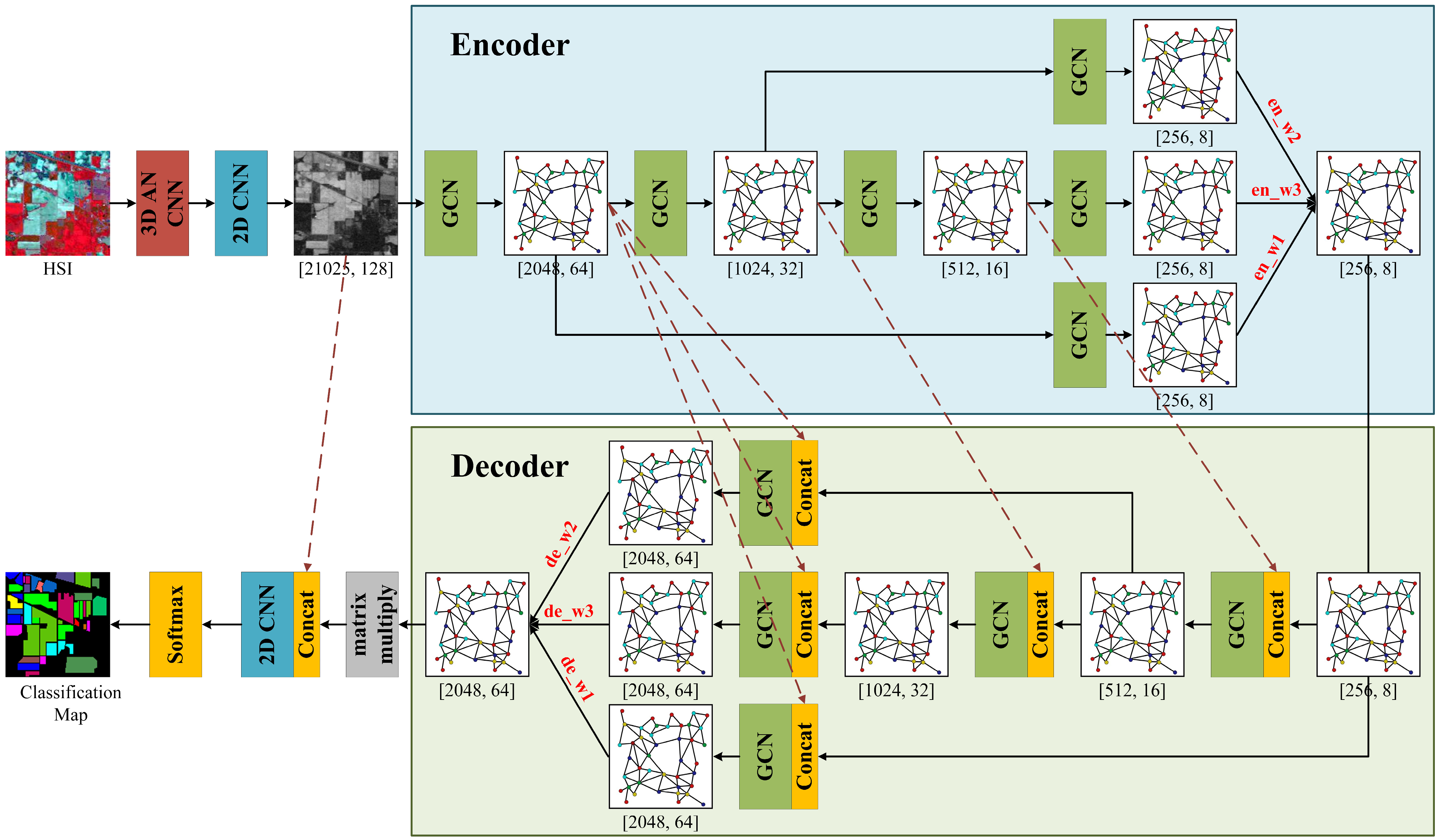
Figure 1 illustrates the framework of the proposed MFSGCN. First, the original image is segmented with different scales of superpixels, edges are created between adjacent superpixels, and each superpixel is averaged as a node of the graph. Then, the pixel-level features of the input HSIs are extracted using CNNs to alleviate the huge computational effort caused by the pixel-level graph structure. The spectral and spatial features of the image are extracted using 3D asymmetric decomposition convolution, which allows differently sized convolution kernels in the spectral and spatial dimensions, thereby enhancing network depth while reducing parameters. The spatial features at the pixel level are further extracted using the 2D CNN, and the obtained feature maps are used as the input to the graph structure. Next, the superpixel feature maps at different scales are coded and fused from fine to coarse using GCNs, and different weights are automatically assigned to the features at different scales by means of a feature search during the fusion process. The decoding process is the opposite of encoding, where features are decomposed from coarse to fine in reverse, and then the final graph structure features are obtained by summing and fusing the weights. Finally, the final graph structure features are converted into pixel-level features by matrix multiplication, and then classified by fully connected layers to obtain classification results.

Figure 1.
Framework of the multiscale feature search-based graph convolutional network (MFSGCN) for HSIC.
In the figure, 2048, 1024, 512, and 256 are empirically set numbers of superpixels in different scale graph structures. Furthermore, 64, 32, 16, and 8 represent the number of feature graphs at different scales, while 128 denotes the number of pixel-level feature maps entered at the very beginning. There, en_w1, en_w2, and en_w3 represent the weight values corresponding to the graph structure where the superpixels go from small to large and the features go from fine to coarse (i.e., the scale shifts from 2048, 1024, and 512 to 256 on) during the encoding process; de_w1, de_w2, and de_w3 represent the weight values of the graph structure with large to small superpixels and coarse to fine features during the decoding process.
2.1. Three-Dimensional Asymmetric Decomposition Convolutional Neural Networks
The 3D asymmetric decomposition convolution has a deeper structure and fewer parameters than the traditional 3D convolution with the same field of perception. For hyperspectral data with low spatial resolution and a high spectral resolution level, the size of the convolution kernels along the spatial and spectral dimensions are theoretically different, and applying the same size kernel in the spatial and spectral dimensions will result in too many parameters and affect the final classification performance, while decomposing the ordinary 3D convolution into a pseudo-3D convolution along the spatial and spectral dimensions can increase the size of the kernel without increasing the parameters of the computation. For example, a 3 × 3 × 3 sized 3D convolution kernel has 27 parameters, and increasing the kernel size to 5 along the spectral dimension will increase the number of parameters to 5 × 3 × 3 = 45, while the corresponding 3D asymmetric decomposition convolution has 1 × 3 × 3 + 5 × 1 × 1 = 14 parameters, which is less than 1/3 of the parameters of an ordinary 3D convolution. A 3D asymmetric decomposition convolutional neural network is used in this paper. The structure includes the LeakyReLU activation function, the spatial dimensional 3D decomposed convolution Conv3d (1 × 3 × 3), the spectral dimensional 3D decomposed convolution Conv3d (3 × 1 × 1), and the batch normalization function BatchNorm3d. Compared with the ReLU function, which forcibly sets all negative values to 0, LeakyReLU preserves the non-zero gradient with a small slope for negative values. This avoids the problem of the “death” of neurons in the ReLU function, i.e., the gradient disappears to zero when backpropagating, and the weights and bias parameters cannot be updated.
2.2. Multiscale Superpixel Structure Graph
Superpixels are irregular blocks of pixels composed of neighboring pixels with similar texture, color, luminance, and other features. Using a small number of superpixels instead of a large number of pixels to express the features of an image largely reduces the complexity of image post-processing. In this chapter, the simple linear iterative clustering (SLIC) segmentation algorithm is chosen to perform superpixel segmentation on the original HSIs. SLIC requires fewer manually adjustable parameters, typically using only one parameter to set the default number of pre-segmented superpixels. Compared with other superpixel segmentation methods, SLIC operates faster, produces more compact and orderly superpixels, maintains well-defined contours, and accurately captures neighborhood features [27]. In this paper, the original HSIs are constructed according to a prediction using a progressive superpixel merging technique to construct multilayer superpixel structure graphs for developing spatial topological relationships at different scales. Suppose the graph structure generated by HSI segmentation is denoted by , where each superpixel is averaged into a node v, , and edges ε, , are established between adjacent nodes, and finally a superpixel structure graph containing N nodes and M edges can be obtained. In this way, we can further construct graphs with different numbers of nodes at different levels, and these graphs can be used to reveal the spatial topology of images at different scales. By using the progressive merging relation in hierarchical superpixels, where any larger superpixel is generated by merging a set of smaller superpixels, a multilayer superpixel structure graph can be constructed.
2.3. Neural Architecture Search
NAS algorithms distinguish themselves from traditional deep learning image algorithms by automating the discovery of high-performance neural architectures instead of relying on manually designed network frameworks. NAS methods have been applied extensively across various domains including image classification [28], semantic segmentation [6], target detection [29], image denoising [30], and computer vision [31], and other fields have received extensive attention. The research on structural search of neural networks focuses on the determination of the search space and search strategy.
The search space is a collection of networks consisting of parameters such as the depth of the network structure, the type of operations, the type of connections, the size of the convolutional kernel, and the number of filters. Within the collection, various operations are combined to produce different network architectures, thus building a suitable search space to facilitate efficient finding of the best network structure. The search space is further distinguished into the macro search space and the micro search space according to the structure of spatial units. The macro search space is based on the artificially set number of network layers for network training and parameter optimization, and mostly uses a chain structure or multi-branch structure. The micro search space is designed with a cell structure as the basic spatial unit. Each cell contains several selection blocks, each representing different functions and operations. Using the cell as the basic unit of spatial stacking reduces the search cost in the process of searching and increases the diversity of the search space at the same time. Cell-based search is built by repeatedly stacking fixed structures for network construction, and such repeatedly stacked structures are called cells (Cell) or selection blocks (Block), which contain basic operations such as convolution, pooling, and skip connection. The stacking of multiple small cells to form a larger network architecture is a super search network. A common 18-layer ResNet is a stack of 18 basic residual blocks. The cell-based search strategy searches through several different supercells, in which each path has all candidate operations, and each candidate operation corresponds to a learnable weight. The supercell with the best performance is obtained as the structure of this network layer via the updated weights, and finally these network layers are stacked in order to build the final optimized network.
The goal of the search strategy is to use the most effective search algorithm to search the network structure, efficiently and accurately find the optimal combination of network structures, and optimize the parameters. Currently, the main search strategies are reinforcement learning-based strategies, evolutionary algorithm-based strategies, Bayesian optimization, and gradient-based architecture search, as follows. (1) Neural structure search based on reinforcement learning mainly guides the next learning behavior after getting feedback by communicating with the environment; for example, using RNNs to feed back the accuracy of the validation set and cyclically optimize the network. (2) Evolutionary algorithms are based on genetic coding, population initialization, cross-variance operators, and retention mechanisms in biology, and iteratively evolve the initial population until the fitness condition is met. (3) Bayesian optimization is one of the main strategies currently used for hyperparametric optimization, mainly using Gaussian processes and kernel methods to solve high-dimensional optimization problems, and the optimization process uses tree models or random forests. (4) Gradient-based methods are the most classical methods in the field of machine learning; these are faster and more efficient than the previous methods and can save training time.
2.4. MFSGCN
In view of the complex design of the network model of NAS and the long training time, we only use the mechanism of neural network search in the structure of the multiscale graph convolutional neural network, remove the complex unit structure that is repeated many times from the neural structure search network, only search the graph structure of different levels in the hyperspectral image, seek the optimal graph structure features for classification, and achieve the purpose of automatically selecting the optimal graph.
The network structure of MFSGCN is divided into two major parts: pixel-level feature extraction and superpixel-level feature extraction. Pixel-level feature extraction is performed using a 3D asymmetric CNN and a 2D CNN. The data after the 2D CNN are transformed into the input matrix of graph convolution . The superpixel feature extraction is further subdivided into the encoding process and the decoding process, where the multiscale feature search algorithm is applied to the fusion of the graph encoding and the decomposition of the graph decoding, respectively. In the graph coding process, the shallow superpixel structure graph is gradually fused into the deep superpixel structure graph. A total of four layers of superpixel structure graph are designed for feature extraction, denoted . N denotes the number of nodes in the graph, and . The matrix representing the graph structure features is denoted . In the fusion process, a pooling operation is used, and all the shallow graphs are fused into the deepest graph after the graph convolution operation. The transformation equation is:
where is the pooling function. represent the feature maps of the 2nd, 3rd, and 4th layer superpixel structure maps after the pooling operation, respectively. They have the same size as the feature maps in layer 5, which is the deepest layer. The feature map of the deepest layer is obtained by summing the feature maps of the previous layers. The optimal weights en_w1, en_w2, and en_w3 are searched for in the deepest layer of graph structure features using the NAS algorithm. When the loss and overall accuracy of the network reach the best at the same time, the weights at this time are the optimal weights, which will be saved and returned. The calculation formula of the deepest feature map is:
The decoding process of graph structure features is the opposite of the encoding process, where all deep graphs are decomposed into the shallowest ones after the graph convolution operation. The process uses the operation of inverse pooling:
where is the inverse pooling function. represent the layer 2, 3, and 4 superpixel structure maps in the decoding process, respectively. represent the feature maps with the same feature scale as the 2nd layer, i.e., the shallowest layer, after inverse pooling by , respectively. The feature maps of the shallowest layer are also obtained by summing the features of the previous layers. Mirroring the encoder, the optimal weights de_w1, de_w2, and de_w3 are searched for in the graph structure features of the shallowest layer using the NAS algorithm. The calculation formula is:
For convenience, the connection weights of GCN layers in the encoder can be defined as α, and the connection weights of GCN layers in the decoder can be defined as β. Specifically, α = {en_w1, en_w2, en_w3}; β = {de_w1, de_w2, de_w3}. By using these parameters to calculate the weighted sum during the forward propagation of the model, we can control the information flow between different layers. During the search process, these connection weights α and β are optimized using gradient descent so that the final network output minimizes a predefined loss function. After learning and optimization, the GCN layer with optimal α and β values is found to determine the final graph structure features and used in the final classification to obtain the classification result map.
To be specific, we use overall accuracy (OA) and loss to evaluate the performance of the search. In order to simplify the calculation process and improve computational efficiency, the loss computed during the network training process is based on the cross-entropy loss function. For HSI with C classes, the number of training samples for the class is assumed as (1 ≤ c ≤ C). The loss for the class is represented as:
Here, is the value of pixel n in the true label (one-hot) of the sample for the class, is the predicted probability of pixel n for the class in the network output, and is the total number of training samples. Then, can be calculated by:
where is the number of pixels whose network output matches the true label and belongs to class c, and is the total number of pixels in class c.
The search process for the multiscale graph convolutional neural network is shown in Algorithm 1.
| Algorithm 1 Multiscale Graph Convolutional Neural Network Searching | |
| Input: | The GCN layers . |
| 1: | Initialize the GCN layers and search weight parameters and for the encoder and decoder. |
| 2: | Set the search procedure parameters. |
| (1) Set the initial optimal accuracy and minimum loss to 0 and infinity. | |
| (2) Set the initial optimal GCN connection structure {α,β} to 0. | |
| (3) Set the epochs of searches to T (T = 100). | |
| 3: | for iter in range (0,T) do |
| 4: | Optimize the current GCN connection weight {α,β}; |
| 5: | Calculate the current search loss and accuracy by Equations (15) and (16) respectively; |
| 6: | Update the GCN connection weight ; |
| 7: | Compare the values of and with and : |
| If > , the and are updated, and the current weight {α,β} is saved. | |
| If = ∧ < , the is updated and the current weight {α,β} is saved. | |
| 8: | end for |
| 9: | Save the model parameters with the best accuracy . |
| Output: | Optimal GCN connection weight {α,β}. |
3. Experimental Results
In this section, we first present three experimental datasets and analyze the trends of the weight ratios of the multiscale features. After that, the results are compared with some state-of-the-art deep learning methods to fully demonstrate the advantages of the proposed algorithm. Finally, we discuss the impact of each module on the model and the computational cost of the model.
3.1. Datasets
Three common HSI datasets, i.e., Indian Pines, Pavia University, and Salinas, were considered in our experiments, as listed in Table 1. The numbers and names of each category, the number of training samples, and the total number of category samples for each of the three datasets are listed in Table 2. The false color image, ground truth map, and color code are depicted in Figure 2.

Table 1.
List of three datasets.
Table 2.
Number of training and total samples for the three datasets.
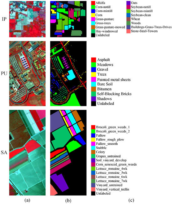
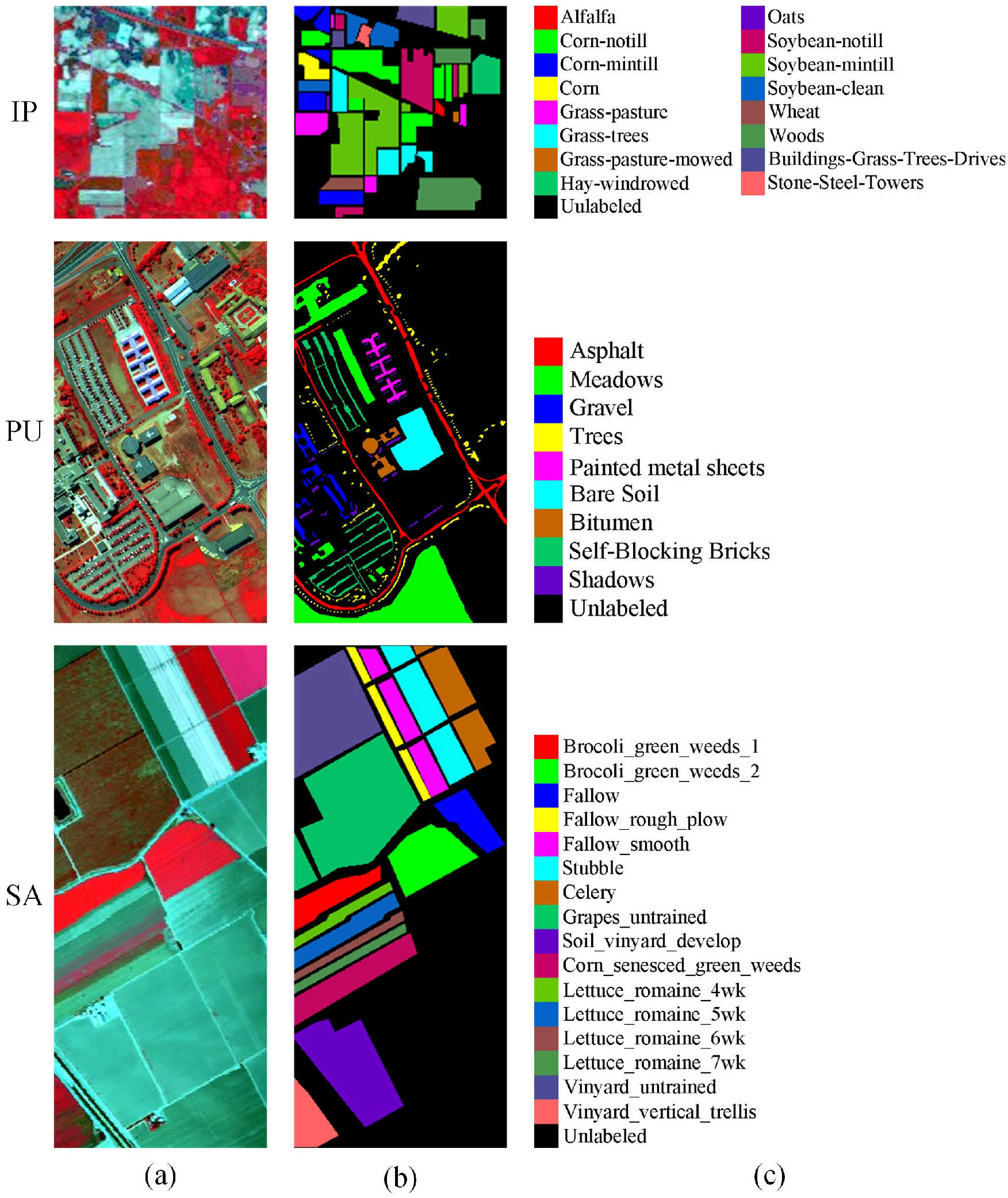
Figure 2.
Graphical illustration of Indian Pines (IP), Pavia University (PU), and Salinas (SA). (a) False-color map. (b) Ground-truth map. (c) Color code.
- Indian Pines (IP): This dataset was captured by an AVIRIS sensor in Northwestern Indiana on June 1992. It contains 145 × 145 pixels with 20 m spatial resolution, and there are 224 spectral bands in the wavelength range of 0.4–2.45 µm. After removing the bands affected by atmospheric absorption, 200 bands are used for classification. The ground truth contains 16 vegetation classes with 10,249 labeled pixels.
- Pavia University (PU): This dataset was acquired by a ROSIS sensor over Pavia University, Northern Italy, in July 2002. There are 103 spectral bands in the spectral range from 0.43 to 0.86 µm obtained by removing several noise-corrupted bands. It contains 610 × 340 pixels with a 1.3 m spatial resolution. This dataset contains nine distinguishable urban classes.
- Salinas (SA): The Salinas dataset was acquired by an AVIRIS sensor over the Salinas Valley, California, USA. It contains 512 × 217 pixels with a 3.7 m spatial resolution and 224 bands in the spectral range of 0.36–2.5 µm. Similar to the IP scene, 20 water-absorbing bands were discarded, and 204 bands were retained. In addition, it contains 16 ground-truth classes.
3.2. Experimental Settings
We evaluated the performance of the proposed model on a server with an NVIDIA GeForce RTX 3090 GPU with 24 GB RAM. The code implementation of all methods is based on Python 3.6 with the PyTorch 1.7 library. Two CNN layers are used to extract pixel-level features both after the input and before the final result output, with kernel sizes of 1 × 1 and 5 × 5, respectively. The optimizer used was Adam, with the learning rate set to 5 × 10⁻⁵ for the weight search process and 5 × 10⁻⁴ for the training process in the MFSGCN method. Several evaluation indicators, including class-specific accuracy, overall accuracy (OA), average accuracy (AA), and kappa coefficient (kappa), are used to evaluate the proposed method exactly. Three publicly available hyperspectral datasets were selected for experimental validation, namely IP, PU, and SA. About 5% of the samples were randomly selected as the training and validation sets for the IP data and the remaining data were used as the test set, while 0.5% of the samples were randomly selected as the training and validation sets for the PU and SA data and the remaining data were used as the test set. For the category with fewer samples, at least two samples were randomly selected as the training and validation sets, and the other samples were used as the test set.
The proposed MFSGCN model was compared with seven representative state-of-the-art HSIC algorithms, namely 3D CNN [11], SSRN [32], HybridSN [33], A2S2K-ResNet [34], MDGCN [15], CEGCN [2], and MSSGU [1]. The first four algorithms are deep learning methods based on CNN, and the optimal model was obtained by training 100 times in each experiment. MDGCN, CEGCN, MSSGU, and MFSGCN are GCN-based deep learning methods, which were trained 300 times per experiment to obtain the optimal model for testing. The experiments were repeated five times for each method to eliminate the bias of the randomly selected training samples, and the mean accuracy and standard deviation of each evaluation criterion were recorded. The above methods are described in detail as follows.
- 3D CNN: A method for direct extraction of spectral and spatial information using 3D convolutional operations; the network contains a 3D convolutional layer, a pooling layer, and a fully connected layer.
- SSRN: A deep CNN that uses spectral residual blocks and spatial residual blocks to extract discriminative spectral and spatial features.
- HybridSN: A hybrid CNN algorithm that combines a 3D CNN for extracting spectral and spatial features with a 2D CNN for extracting abstract spatial features.
- A2S2K-ResNet: A spectral spatial residual neural network that combines a spectral spatial attention mechanism with the ability to adaptively select the size of the kernel, and employs an efficient feature recalibration mechanism to improve classification performance.
- MDGCN: A dynamic GCN based on superpixel segmentation for HSIC.
- CEGCN: A neural network that simultaneously learns small-scale pixel-level features using a CNN and large-scale super-pixel-level features using a GCN and combines the two.
- MSSGU: A GCN that learns features at different levels and scales of superpixel structured graphs from coarse to fine, and uses CNN to extract pixel-level features and reduce computational effort.
3.3. Variation of Multiscale Feature Weight Values
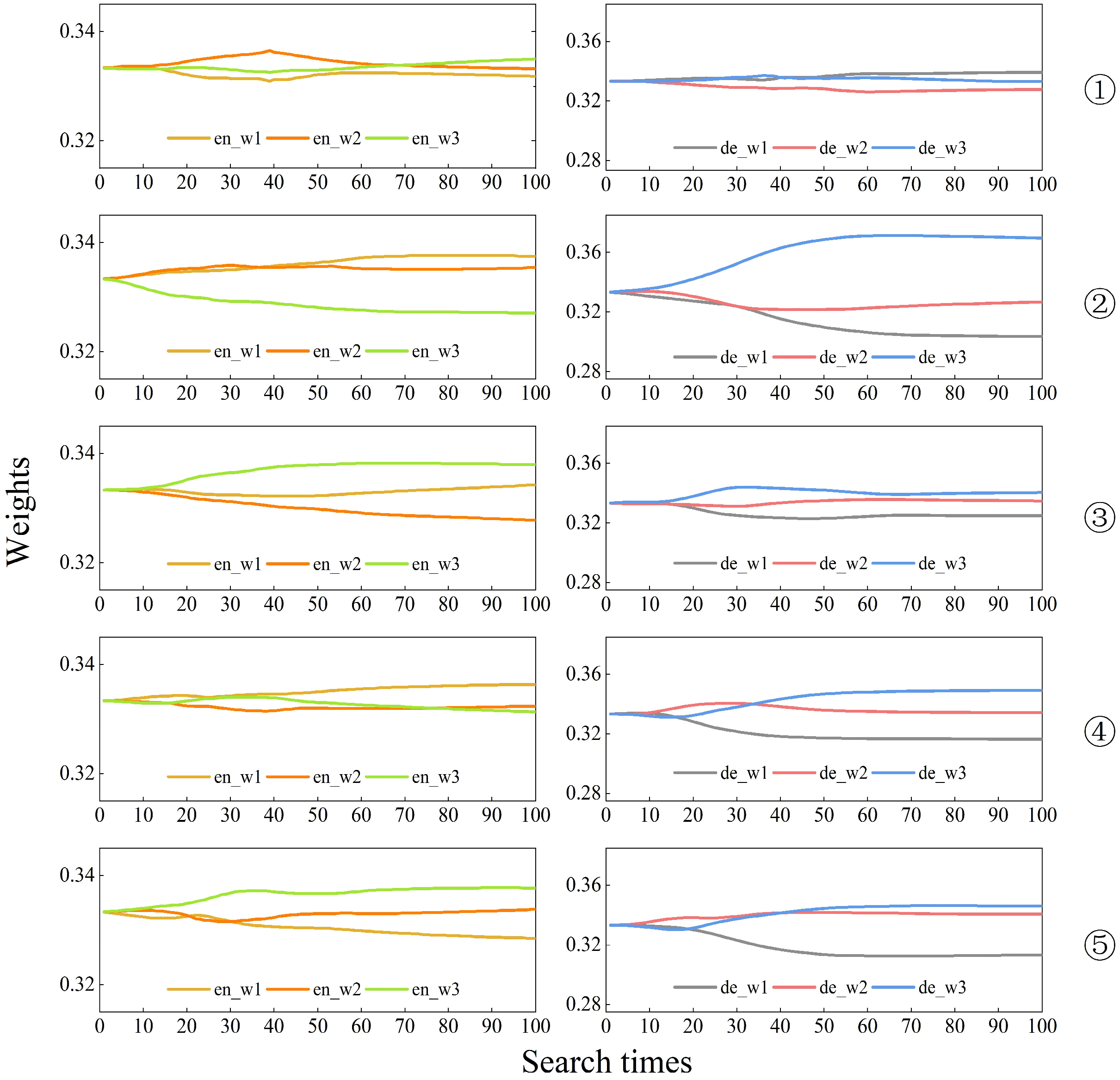
Figure 3, Figure 4 and Figure 5 show the graphs of the variation of the weight values of the multiscale features with the number of searches in the process of searching the IP, PU, and SA datasets, respectively.
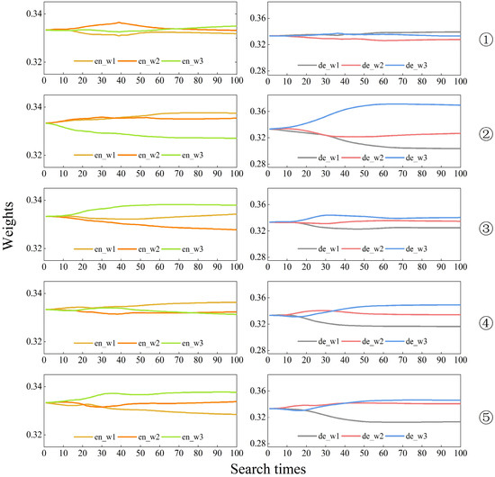
Figure 3.
Multiscale feature weights of IP dataset search process. The experiments were repeated five times for the weights of encoder and decoder, respectively.
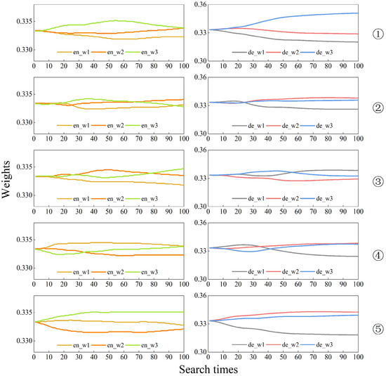
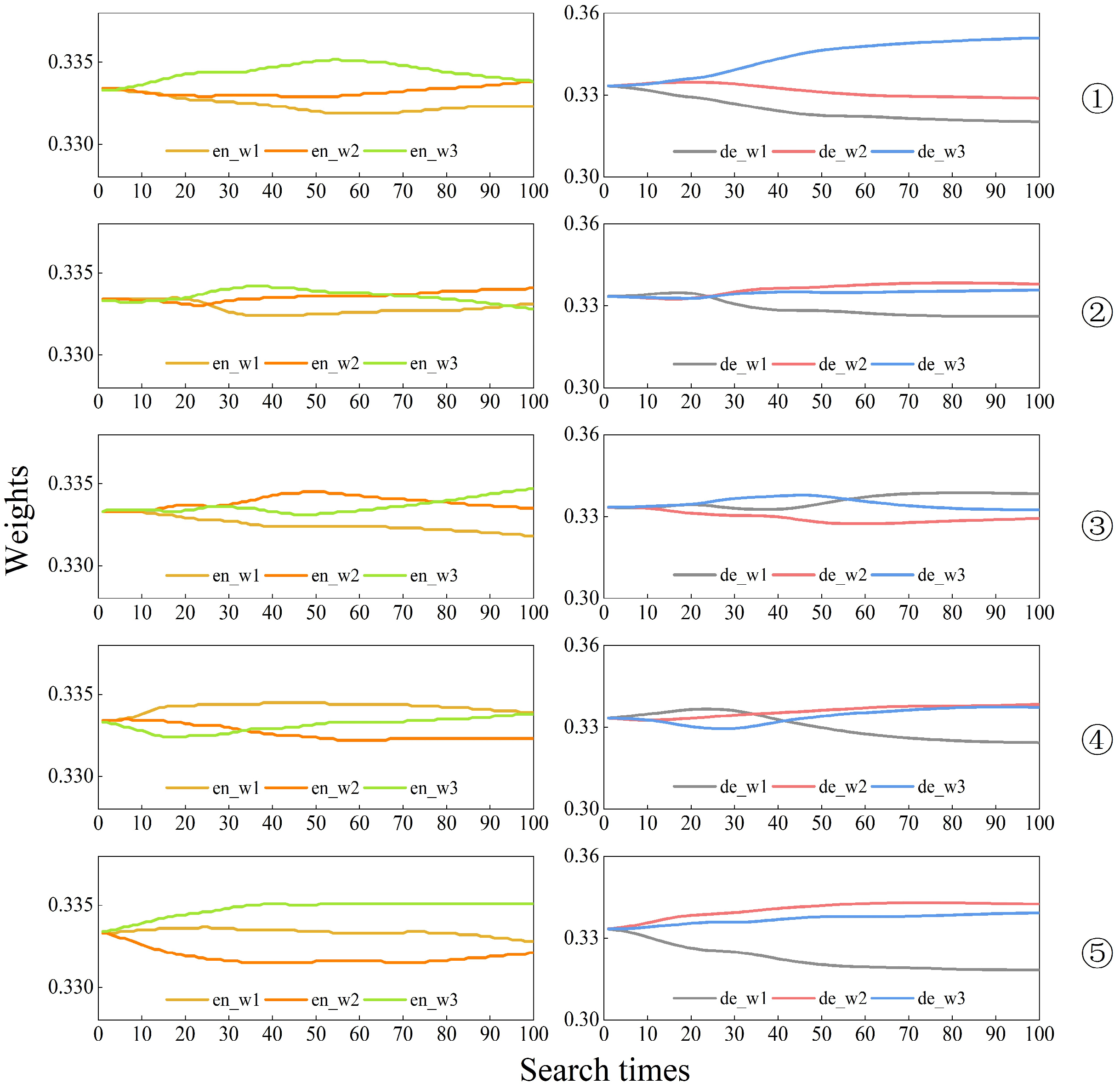
Figure 4.
Multiscale feature weights of PU dataset search process. The experiments were repeated five times for the weights of encoder and decoder, respectively.
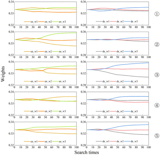
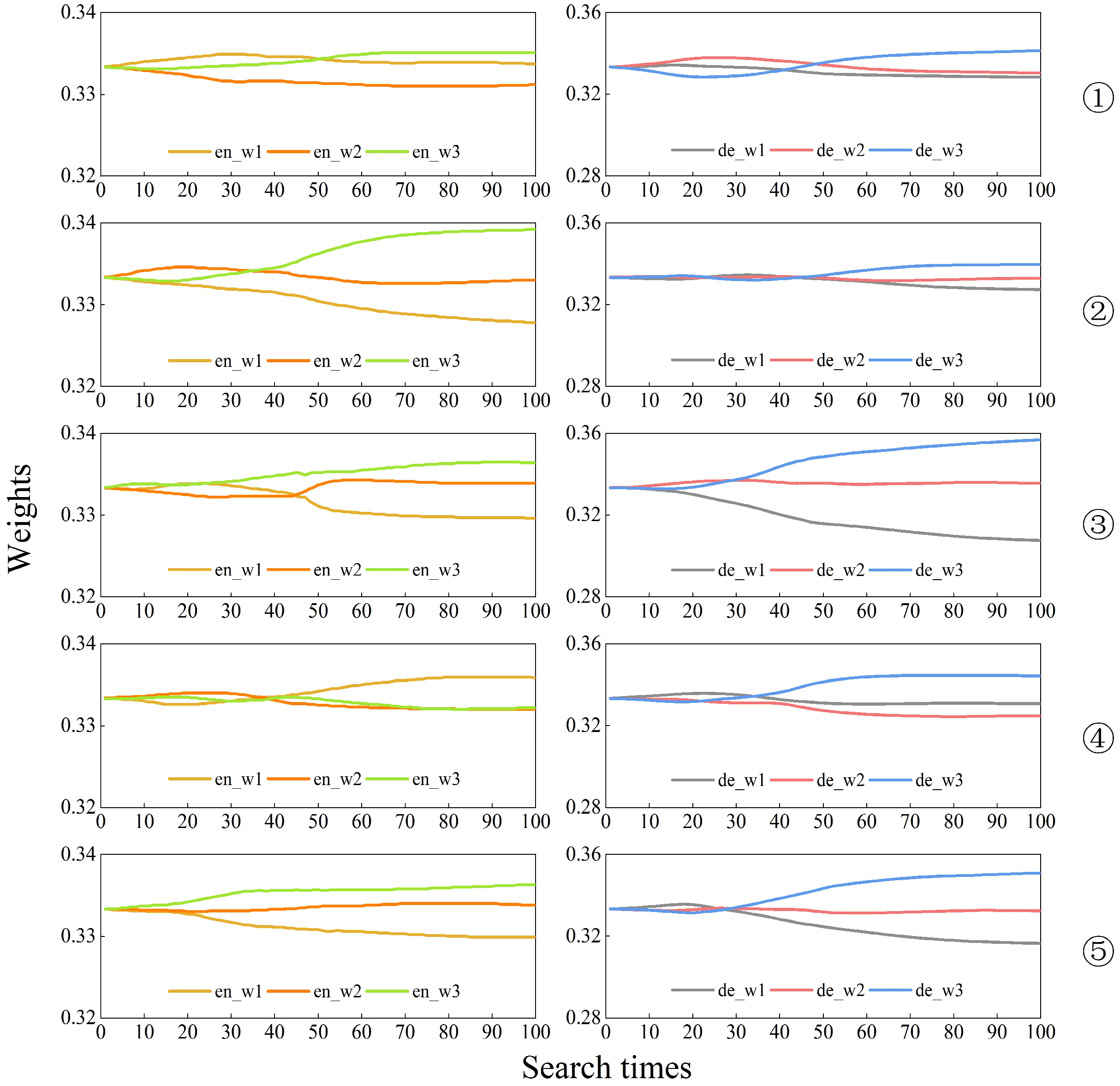
Figure 5.
Multiscale feature weights of SA dataset search process. The experiments were repeated five times for the weights of encoder and decoder, respectively.
In the figures, en_w1, en_w2, and en_w3 represent the weights of the graph structure features corresponding to the model in the process of encoding from small to large superpixel scales, i.e., from fine to coarse features, respectively. These three weights are obtained by applying the SoftMax function, ensuring that their sum is equal to 1. On the other hand, de_w1, de_w2, and de_w3 represent the weights of the feature graphs corresponding to the model in the process of decoding from large to small superpixel scales, and the weights are also generated through the SoftMax function, ensuring that their sum is equal to 1.
In the actual search process, the optimal weight combination of the encoder and decoder can produce the highest accuracy and minimal loss weights for model training in the set 100 training cycles. The experiments were repeated five times for each dataset, and it can be seen from Figure 3 and Figure 4 that the results of the weights searched for in each experiment are inconsistent. This indicates that when extracting image features using GCNs, it is not the case that the larger or smaller the scale of the superpixels, the more useful information it contains. In contrast, the multiscale feature search model we designed can focus attention on the feature layers with more information and assign higher weights to the informative feature layers, thus automating the classification process. Furthermore, the repeated experiments from the second to the fifth iteration on the IP dataset, as well as the five repeated experiments on the SA dataset, indicate that as the number of iterations increases, de_w3 tends to obtain the highest weight value. This phenomenon shows that the deepest feature maps that have undergone the process of fine to coarse feature fusion and coarse to fine feature decoding are the most informative and most representative of the attribute classes of the features.
In summary, the main function of the encoder is to learn and understand the feature representations of the input data, which can vary depending on the dataset or training. Therefore, this process may not create a consistently stable pattern of weight distribution. In the weight distribution of the decoder, the weight of the last layer often accounts for a larger proportion. After conducting a weight search for 100 epochs, the optimal weights obtained were the weights from a specific epoch where the model achieved the best loss and accuracy. The weights en_w1, en_w2, and en_w3 in the encoder module were 0.3316, 0.3378, and 0.3306 for IP data; 0.3356, 0.3338, and 0.3306 for PU data; and 0.3311, 0.3345, and 0.3345 for SA data. Furthermore, the weights de_w1, de_w2, and de_w3 in the decoder module were 0.3356, 0.3338, and 0.3306 for IP data; 0.3335, 0.3346, and 0.332 for PU data; and 0.3164, 0.3332, and 0.3504 for SA data. The model’s state and these weights at that moment were saved for future classification tasks.
3.4. Classification Results
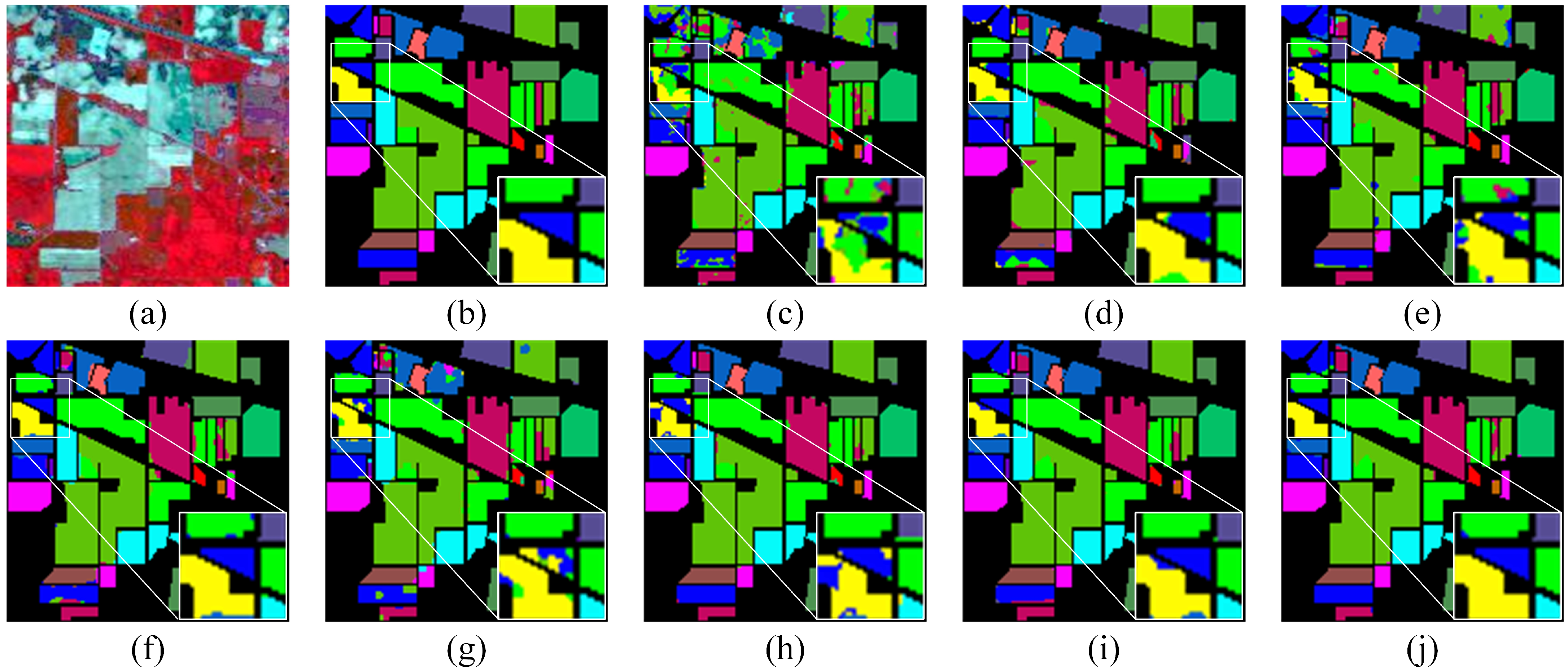
Figure 6 shows a graph of the classification results for the IP dataset and zooms in on the detailed features for more direct observation and comparison. As can be seen from the figure, the MFSGCN method proposed in this chapter visually obtains the best classification results, with almost no misclassifications, and the details show that MFSGCN outperforms the other methods in terms of classification results. In addition, the algorithms A2S2K-ResNet and MSSGU also both achieved good classification results with fewer misclassified pixel points, while the other algorithms clearly had worse classification results with more misclassification. Table 3 shows the specific classification accuracies for the IP dataset, including OA, AA, kappa, and category classification accuracy, each judged by averaging over five experiments, so the table also shows the standard deviation values. The bold text is the highest accuracy among all of the categories in the table. It is clear that MFSGCN has the highest OA, AA, and kappa of the eight methods, with MFSGCN having an OA value of 98.44%, AA of 98.64%, and kappa of 98.22%. MFSGCN also has the smallest standard deviation of all methods for the three metrics, with a standard deviation of only 0.14% for OA, indicating the highest stability of the method. In addition, 10 of the 16 categories have the highest classification accuracy, with category 12 having the most significant accuracy improvement, outperforming the MSSGU results by 4.26%. As the GCN processes the whole image directly, it focuses on the overall improvement in accuracy, outperforming other classification methods.

Figure 6.
Classification maps for the IP dataset. (a) False-color image. (b) Ground truth. (c) 3D CNN. (d) SSRN. (e) HybridSN. (f) A2S2K-ResNet. (g) MDGCN. (h) CEGCN. (i) MSSGU. (j) MFSGCN.
Table 3.
Classification results of the IP dataset (%).
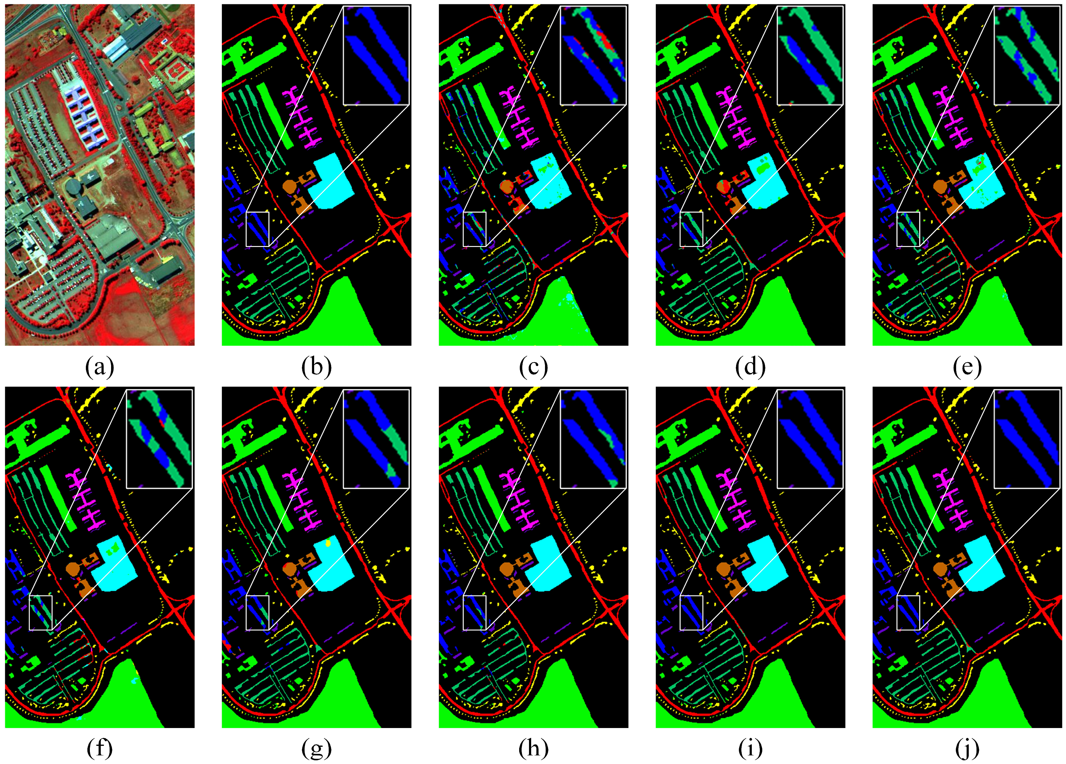
The experimental results for the PU dataset are shown in Figure 7. Comparing the classification reference map with the classification results of all methods shows that the MFSGCN algorithm has more detailed processing and more accurate classification. All the algorithms except the proposed MFSGCN method and MSSGU method showed good classification in detail, while all other methods misclassified some of the gravel (Gravel, blue) as Self-Blocking Bricks (dark green). The classification accuracy of the PU dataset is shown in Table 4, from which it can be seen that MFSGCN has the highest accuracy values, of 99.15% for OA, 99.17% for AA, and 98.87% for kappa, which were 0.56%, 0.88%, and 0.74% higher than those of MSSGU, respectively. Among the nine feature categories, seven of them are those with the highest recognition accuracy, and the lowest accuracy feature category also achieves 96.44% accuracy, proving the advantages of the proposed algorithm. In addition, the standard deviation of OA, AA, and kappa of the method in this chapter is the smallest among all the methods, which is less than 0.5%, and the standard deviation of accuracy within most of the other methods is greater than 1%. This indicates that the method has high stability and can accurately identify the target feature types.
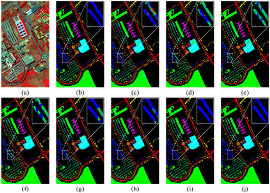
Figure 7.
Classification maps for the PU dataset. (a) False-color image. (b) Ground truth. (c) 3D CNN. (d) SSRN. (e) HybridSN. (f) A2S2K-ResNet. (g) MDGCN. (h) CEGCN. (i) MSSGU. (j) MFSGCN.
Table 4.
Classification results of the PU dataset (%).
The classification results of the SA dataset are shown in Figure 8. It can be seen that the proposed MFSGCN method showed better classification results both overall and in terms of local details, generating the most accurate and smoothest classification maps with only very few pixel points being misclassified. The other classification methods showed poorer classification results, mainly on the two main classes “Vinyard_untrained” and “Grapes_untrained” (top left part of the figure). The MFSGCN method also had the highest OA, AA, and kappa classification results, of 99.54%, 99.31%, and 99.49%, respectively, (see Table 5), which were higher than those of MSSGU by 0.49%, 0.38%, and 0.55%. The overall classification accuracy of 99.54% was obtained with 0.5% of the training samples, proving that the proposed algorithm can extract effective information from very few training samples and obtain high classification accuracy, solving the problem of difficulty in obtaining labeled samples from HSIs. In addition, among the other compared methods, the simple 3D CNN obtained the lowest OA of 92.5%; SSRN, HybridSN, and A2S2K-ResNet obtained 94.44%, 94.67%, and 95.63% classification accuracies, respectively; while the GCN-based MDGCN, CEGCN, and MSSGU classification methods obtained 97.65%, 98.88%, and 99.05% classification accuracies, respectively, outperforming the CNN-based classification methods and proving that the graph structure has certain advantages in HSIC.
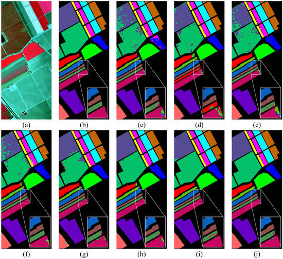
Figure 8.
Classification maps for the SA dataset. (a) False-color image. (b) Ground truth. (c) 3D CNN. (d) SSRN. (e) HybridSN. (f) A2S2K-ResNet. (g) MDGCN. (h) CEGCN. (i) MSSGU. (j) MFSGCN.
Table 5.
Classification results of the SA dataset (%).
3.5. Ablation Study
To further validate the effectiveness of the different modules in the MFSGCN network, we conducted ablation experiments while keeping the other experimental settings unchanged. The ablation study included a multiscale GCN, encoder feature search, decoder feature search, and 3D asymmetric decomposition convolution. Table 6 shows the OA classification results of the ablation experiments. As can be seen from the table, the inclusion of the feature search structure in the encoder and decoder greatly improves the accuracy compared to the underlying multiscale GCN, with the accuracy of the datasets IP, PU, and SA improving by 0.55%, 0.41%, and 0.37%, respectively, compared to the multiscale GCN, due to the multiscale feature search module extracting diagnostic spectral and spatial feature information, which improves the accuracy of feature recognition. In addition, we analyzed the role of the 3D asymmetric decomposition convolution module, and the results show that the inclusion of 3D asymmetric decomposition convolution is also important for OA enhancement, with the accuracy of the IP, PU, and SA datasets improving by 0.23%, 0.09%, and 0.24%, respectively. This shows that the inclusion of multiscale feature search patterns and 3D asymmetric decomposition convolution can obtain more effective features, which is important for the improvement of classification accuracy.
Table 6.
Analysis of the accuracy of OA for different modules of the proposed framework.
3.6. The Limitation of MFSGCN
Table 7 shows the complexity of the different methods in terms of training time, the number of trainable weight parameters, and the computational cost. Due to the search mechanisms, the proposed algorithm requires more training time than the other methods. Specifically, the training time for PU is the highest, at 166.21 s. Therefore, the model has clear limitations regarding training time. Additionally, high FLOPs and a large number of parameters are unavoidable during the process. Compared with the four traditional CNN models and three GCN models, MFSGCN adopts complex processes, including superpixel segmentation, multiscale feature fusion, gradient-based search, and an encoding–decoding module. Even so, the computational cost is still smaller than that of CEGCN, and the number of network parameters used for training is comparable to that of CEGCN. In summary, MFSGCN requires the highest cost in terms of computational time, but it is still acceptable.
Table 7.
Computational cost of the three datasets.
3.7. Analysis and Discussion
First, we explored the role of search structure in multiscale graph convolution and analyze the change in feature weights during feature search for the three datasets. The experiments showed that the goal of multiscale feature graph search is to be able to extract feature layers with more information, rather than simply determining whether the feature layer with more information is composed of larger or smaller superpixels. In other words, our search model can automatically acquire the feature layer with the most information for classification and automate the feature selection operation.
Second, the proposed MFSGCN model was compared with typical CNN and GCN-based methods, and the OA, AA, kappa, and category accuracy values of the three datasets were analyzed. MFSGCN showed the best classification results on all three datasets, IP, PU, and SA, with OA of 98.44%, 99.15%, and 99.54% for the three datasets, respectively, AA of 98.64%, 99.17%, and 99.31%, and kappa of 98.22%, 98.87%, and 99.49%, respectively. In addition, the algorithm has high stability, and the standard deviations of OA, AA, and kappa are less than 0.6% in the experimental results from the three datasets. The main advantages of the algorithm are that it can automatically select the multiple scales with the maximum amount of information for the classification task and obtain an overall classification accuracy of more than 98% using very few training samples.
Third, the role of individual structures in the model was demonstrated based on ablation experiments. The inclusion of feature search in the encoder and decoder as well as the 3D asymmetric decomposition convolution module are effective for the accuracy improvement. We also analyzed the computational cost and time consumption of the model, showing that our model does not add much computational effort.
4. Conclusions
In this paper, we propose a multiscale feature search-based graph convolutional neural network (MFSGCN) for HSIC. The method first extracts pixel-level features of HSIs using 3D asymmetric decomposition convolution and 2D convolution operations. Then, the large-scale super-pixel level features are extracted using multiscale GCNs. Concurrently, the NAS algorithm is employed to explore features across different scales of superpixel structure maps, automatically assigning varying weights to these features to enhance the discriminative power of the resulting feature maps for classification. Adequate experiments on three widely used HSI datasets show that the proposed MFSGCN model surpasses the state-of-the-art methods, achieving superior classification accuracy. The experiments show that MFSGCN effectively learns optimal features for classification, even with limited data samples. Considering that the proposed model is a supervised learning classification method, in future research, we will explore semi-supervised and unsupervised approaches, as well as novel network architectures, to further enhance the intelligence and accuracy of hyperspectral classification for broader applications.
Author Contributions
Conceptualization, K.W.; methodology, K.W. and Y.Z.; formal analysis, K.W., Y.A. and S.L.; writing—original draft preparation, K.W. and Y.Z.; writing—review and editing, K.W., Y.A. and S.L.; funding acquisition, K.W. and Y.A. All authors have read and agreed to the published version of the manuscript.
Funding
This research was funded by the National Natural Science Foundation of China, grant number U21A2013; the Foundation of State Key Laboratory of Public Big Data, grant number PBD2023-28; the State Key Laboratory of applied optics, grant number SKLAO2021001A01; the Hebei Key Laboratory of Ocean Dynamics, Resources and Environments, grant number HBHY2302; the S & T Program of Hebei, grant number 21373301D; the Open Fund of Wenzhou Future City Research Institute, grant number WL2023007; the Open Fund of State Key Laboratory of Remote Sensing Science, grant number OFSLRSS202312; the Fundamental Research Funds for the Central Universities, China University of Geosciences (Wuhan), grant number 2642022009; the Global Change and Air-Sea Interaction II under Grant, grant number GASI-01-DLYG-WIND0; the Open Fund of Key Laboratory of Space Ocean Remote Sensing and Application, MNR, grant number 202401001; the Open Fund of Key Laboratory of Regional Development and Environmental Response, grant number 2023(A)003.
Data Availability Statement
These hyperspectral data were derived from the following resources available in the public domain: [Hyperspectral Remote Sensing Scenes, and https://www.ehu.eus/ccwintco/index.php/Hyperspectral_Remote_Sensing_Scenes, accessed on 1 February 2024].
Conflicts of Interest
The authors declare no conflicts of interest.
References
- Liu, Q.; Xiao, L.; Yang, J.; Wei, Z. Multilevel Superpixel Structured Graph U-Nets for Hyperspectral Image Classification. IEEE Trans. Geosci. Remote Sens. 2022, 60, 1–15. [Google Scholar] [CrossRef]
- Liu, Q.; Xiao, L.; Yang, J.; Wei, Z. CNN-Enhanced Graph Convolutional Network With Pixel- and Superpixel-Level Feature Fusion for Hyperspectral Image Classification. IEEE Trans. Geosci. Remote Sens. 2021, 59, 8657–8671. [Google Scholar] [CrossRef]
- Lu, B.; Dao, P.D.; Liu, J.; He, Y.; Shang, J. Recent Advances of Hyperspectral Imaging Technology and Applications in Agriculture. Remote Sens. 2020, 12, 2659. [Google Scholar] [CrossRef]
- Kurz, T.H.; Buckley, S.J.; Howell, J.A. Close-Range Hyperspectral Imaging for Geological Field Studies: Workflow and Methods. Int. J. Remote Sens. 2013, 34, 1798–1822. [Google Scholar] [CrossRef]
- Jänicke, C.; Okujeni, A.; Cooper, S.; Clark, M.; Hostert, P.; van der Linden, S. Brightness Gradient-Corrected Hyperspectral Image Mosaics for Fractional Vegetation Cover Mapping in Northern California. Remote Sens. Lett. 2020, 11, 1–10. [Google Scholar] [CrossRef]
- Weng, Y.; Zhou, T.; Li, Y.; Qiu, X. NAS-Unet: Neural Architecture Search for Medical Image Segmentation. IEEE Access 2019, 7, 44247–44257. [Google Scholar] [CrossRef]
- Chen, Y.; Lin, Z.; Zhao, X.; Wang, G.; Gu, Y. Deep Learning-Based Classification of Hyperspectral Data. IEEE J. Sel. Top. Appl. Earth Obs. Remote Sens. 2014, 7, 2094–2107. [Google Scholar] [CrossRef]
- Zhou, S.; Xue, Z.; Du, P. Semisupervised Stacked Autoencoder With Cotraining for Hyperspectral Image Classification. IEEE Trans. Geosci. Remote Sens. 2019, 57, 3813–3826. [Google Scholar] [CrossRef]
- Zhong, P.; Gong, Z.; Li, S.; Schönlieb, C.-B. Learning to Diversify Deep Belief Networks for Hyperspectral Image Classification. IEEE Trans. Geosci. Remote Sens. 2017, 55, 3516–3530. [Google Scholar] [CrossRef]
- Hang, R.; Liu, Q.; Hong, D.; Ghamisi, P. Cascaded Recurrent Neural Networks for Hyperspectral Image Classification. IEEE Trans. Geosci. Remote Sens. 2019, 57, 5384–5394. [Google Scholar] [CrossRef]
- Chen, Y.; Jiang, H.; Li, C.; Jia, X.; Ghamisi, P. Deep Feature Extraction and Classification of Hyperspectral Images Based on Convolutional Neural Networks. IEEE Trans. Geosci. Remote Sens. 2016, 54, 6232–6251. [Google Scholar] [CrossRef]
- Mei, S.; Chen, X.; Zhang, Y.; Li, J.; Plaza, A. Accelerating Convolutional Neural Network-Based Hyperspectral Image Classification by Step Activation Quantization. IEEE Trans. Geosci. Remote Sens. 2022, 60, 5502012. [Google Scholar] [CrossRef]
- Zhu, L.; Chen, Y.; Ghamisi, P.; Benediktsson, J.A. Generative Adversarial Networks for Hyperspectral Image Classification. IEEE Trans. Geosci. Remote Sens. 2018, 56, 5046–5063. [Google Scholar] [CrossRef]
- Hong, D.; Gao, L.; Yao, J.; Zhang, B.; Plaza, A.; Chanussot, J. Graph Convolutional Networks for Hyperspectral Image Classification. IEEE Trans. Geosci. Remote Sens. 2021, 59, 5966–5978. [Google Scholar] [CrossRef]
- Wan, S.; Gong, C.; Zhong, P.; Du, B.; Zhang, L.; Yang, J. Multiscale Dynamic Graph Convolutional Network for Hyperspectral Image Classification. IEEE Trans. Geosci. Remote Sens. 2020, 58, 3162–3177. [Google Scholar] [CrossRef]
- Hu, H.; He, F.; Zhang, F.; Ding, Y.; Wu, X.; Zhao, J.; Yao, M. Unifying Label Propagation and Graph Sparsification for Hyperspectral Image Classification. IEEE Geosci. Remote Sens. Lett. 2022, 19, 6010305. [Google Scholar] [CrossRef]
- Zhang, H.; Zou, J.; Zhang, L. EMS-GCN: An End-to-End Mixhop Superpixel-Based Graph Convolutional Network for Hyperspectral Image Classification. IEEE Trans. Geosci. Remote Sens. 2022, 60, 5526116. [Google Scholar] [CrossRef]
- Ding, Y.; Zhao, X.; Zhang, Z.; Cai, W.; Yang, N. Multiscale Graph Sample and Aggregate Network With Context-Aware Learning for Hyperspectral Image Classification. IEEE J. Sel. Top. Appl. Earth Obs. Remote Sens. 2021, 14, 4561–4572. [Google Scholar] [CrossRef]
- Xue, Z.; Liu, Z.; Zhang, M. DSR-GCN: Differentiated-Scale Restricted Graph Convolutional Network for Few-Shot Hyperspectral Image Classification. IEEE Trans. Geosci. Remote Sens. 2023, 61, 5504918. [Google Scholar] [CrossRef]
- Yu, L.; Peng, J.; Chen, N.; Sun, W.; Du, Q. Two-Branch Deeper Graph Convolutional Network for Hyperspectral Image Classification. IEEE Trans. Geosci. Remote Sens. 2023, 61, 5506514. [Google Scholar] [CrossRef]
- Elsken, T.; Metzen, J.H.; Hutter, F. Neural Architecture Search: A Survey. J. Mach. Learn. Res. 2019, 20, 55. [Google Scholar]
- Wang, J.; Huang, R.; Guo, S.; Li, L.; Zhu, M.; Yang, S.; Jiao, L. NAS-Guided Lightweight Multiscale Attention Fusion Network for Hyperspectral Image Classification. IEEE Trans. Geosci. Remote Sens. 2021, 59, 8754–8767. [Google Scholar] [CrossRef]
- Liu, X.; Zhang, C.; Cai, Z.; Yang, J.; Zhou, Z.; Gong, X. Continuous Particle Swarm Optimization-Based Deep Learning Architecture Search for Hyperspectral Image Classification. Remote Sens. 2021, 13, 1082. [Google Scholar] [CrossRef]
- Zhang, H.; Gong, C.; Bai, Y.; Bai, Z.; Li, Y. 3-D-ANAS: 3-D Asymmetric Neural Architecture Search for Fast Hyperspectral Image Classification. IEEE Trans. Geosci. Remote Sens. 2022, 60, 5508519. [Google Scholar] [CrossRef]
- Xue, X.; Zhang, H.; Fang, B.; Bai, Z.; Li, Y. Grafting Transformer on Automatically Designed Convolutional Neural Network for Hyperspectral Image Classification. IEEE Trans. Geosci. Remote Sens. 2022, 60, 5531116. [Google Scholar] [CrossRef]
- Chen, Y.; Zhu, K.; Zhu, L.; He, X.; Ghamisi, P.; Benediktsson, J.A. Automatic Design of Convolutional Neural Network for Hyperspectral Image Classification. IEEE Trans. Geosci. Remote Sens. 2019, 57, 7048–7066. [Google Scholar] [CrossRef]
- Gong, Z.; Tong, L.; Zhou, J.; Qian, B.; Duan, L.; Xiao, C. Superpixel Spectral–Spatial Feature Fusion Graph Convolution Network for Hyperspectral Image Classification. IEEE Trans. Geosci. Remote Sens. 2022, 60, 5536216. [Google Scholar] [CrossRef]
- Zhang, Z.; Liu, S.; Zhang, Y.; Chen, W. RS-DARTS: A Convolutional Neural Architecture Search for Remote Sensing Image Scene Classification. Remote Sens. 2022, 14, 141. [Google Scholar] [CrossRef]
- Zhang, H.; Wang, L.; Sun, J.; Sun, L.; Kobashi, H.; Imamura, N. NAS-EOD: An End-to-End Neural Architecture Search Method for Efficient Object Detection. In Proceedings of the 2020 25th International Conference on Pattern Recognition (ICPR), Milan, Italy, 10–15 January 2021; pp. 1446–1451. [Google Scholar]
- Możejko, M.; Latkowski, T.; Treszczotko, Ł.; Szafraniuk, M.; Trojanowski, K. Superkernel Neural Architecture Search for Image Denoising. In Proceedings of the 2020 IEEE/CVF Conference on Computer Vision and Pattern Recognition Workshops (CVPRW), Seattle, WA, USA, 14–19 June 2020; pp. 2002–2011. [Google Scholar]
- Xie, L.; Chen, X.; Bi, K.; Wei, L.; Xu, Y.; Chen, Z.; Wang, L.; Xiao, A.; Chang, J.; Zhang, X.; et al. Weight-Sharing Neural Architecture Search: A Battle to Shrink the Optimization Gap. ACM Comput. Surv. 2021, 54, 1–37. [Google Scholar] [CrossRef]
- Zhong, Z.; Li, J.; Luo, Z.; Chapman, M. Spectral–Spatial Residual Network for Hyperspectral Image Classification: A 3-D Deep Learning Framework. IEEE Trans. Geosci. Remote Sens. 2018, 56, 847–858. [Google Scholar] [CrossRef]
- Roy, S.K.; Krishna, G.; Dubey, S.R.; Chaudhuri, B.B. HybridSN: Exploring 3-D–2-D CNN Feature Hierarchy for Hyperspectral Image Classification. IEEE Geosci. Remote Sens. Lett. 2020, 17, 277–281. [Google Scholar] [CrossRef]
- Roy, S.K.; Manna, S.; Song, T.; Bruzzone, L. Attention-Based Adaptive Spectral–Spatial Kernel ResNet for Hyperspectral Image Classification. IEEE Trans. Geosci. Remote Sens. 2021, 59, 7831–7843. [Google Scholar] [CrossRef]

Disclaimer/Publisher’s Note: The statements, opinions and data contained in all publications are solely those of the individual author(s) and contributor(s) and not of MDPI and/or the editor(s). MDPI and/or the editor(s) disclaim responsibility for any injury to people or property resulting from any ideas, methods, instructions or products referred to in the content. |
© 2024 by the authors. Licensee MDPI, Basel, Switzerland. This article is an open access article distributed under the terms and conditions of the Creative Commons Attribution (CC BY) license (https://creativecommons.org/licenses/by/4.0/).