Abstract
Cloud cover and shadows often hinder the accurate analysis of satellite images, impacting various applications, such as digital farming, land monitoring, environmental assessment, and urban planning. This paper presents a new approach to enhancing cloud-contaminated satellite images using a novel variational model for approximating the combination of the temporal and spatial components of satellite imagery. Leveraging this model, we derive two spatial-temporal methods containing an algorithm that computes the missing or contaminated data in cloudy images using the seamless Poisson blending method. In the first method, we extend the Poisson blending method to compute the spatial-temporal approximation. The pixel-wise temporal approximation is used as a guiding vector field for Poisson blending. In the second method, we use the rate of change in the temporal domain to divide the missing region into low-variation and high-variation sub-regions to better guide Poisson blending. In our second method, we provide a more general case by introducing a variation-based method that considers the temporal variation in specific regions to further refine the spatial–temporal approximation. The proposed methods have the same complexity as conventional methods, which is linear in the number of pixels in the region of interest. Our comprehensive evaluation demonstrates the effectiveness of the proposed methods through quantitative metrics, including the Root Mean Square Error (RMSE), Peak Signal-to-Noise Ratio (PSNR), and Structural Similarity Index Metric (SSIM), revealing significant improvements over existing approaches. Additionally, the evaluations offer insights into how to choose between our first and second methods for specific scenarios. This consideration takes into account the temporal and spatial resolutions, as well as the scale and extent of the missing data.
1. Introduction
Remote sensing is an important technique for gathering information about the Earth’s surface and its processes. Spectral indexing plays a crucial role in remote sensing analysis. However, missing or corrupted pixels in remote sensing data due to factors such as sensor limitations and atmospheric effects can make accurate spectral indexing and subsequent analysis difficult. Satellite imagery is a valuable source of information in various fields, including digital farming, environmental monitoring, disaster assessment, and land-use analysis. However, the presence of cloud cover and shadows can reduce the quality and usability of these images, making it difficult to extract and interpret data accurately. To overcome these challenges, we have developed a comprehensive framework that utilizes both temporal and spatial characteristics to enhance satellite images that are contaminated by clouds.
One approach to addressing the problem of missing data is to use spatial approximation since nearby locations are likely to have similar characteristics. Furthermore, we can expect a continuous variation in the temporal axis for phenomena that change over time, such as vegetation or soil moisture. This temporal aspect can be utilized to enhance the spatial approximation of missing data that may arise due to cloud and shadow masks.
Relying on temporal approximation has been valuable in time-varying remote sensing imagery for understanding dynamic processes on Earth [1,2]. When it comes to spatial approximation, a commonly used and sophisticated method in image processing is Poisson image blending [3]. This technique seamlessly blends two images (source and target) by utilizing the gradient vector field of the source image to smoothly integrate it into the target image. The method involves solving Poisson’s equation to integrate the gradient field, ensuring a smooth and natural transition between the two images [3,4,5].
Methods that combine spatial and temporal information can be used to address missing data in satellite images. However, a more flexible and robust model is needed to handle the variability in temporal and spatial resolutions and also the type and scale of the missing data. Missing data in satellite images can occur in a non-homogeneous region with high or low temporal variation. The availability of temporal imagery can also vary depending on weather conditions and geographic location.
In this paper, we present a novel variational model for the spatial–temporal approximation of time-varying satellite imagery, which is beneficial for addressing missing or masked data caused by clouds and shadows. By using this model, we have developed two novel methods that are useful for potentially different scenarios. The first method extends Poisson inpainting by using a temporal approximation as a guiding vector field for Poisson blending. For the temporal approximation, we use a pixel-wise time-series approximation technique utilizing a weighted least-squares approximation of preceding and subsequent images.
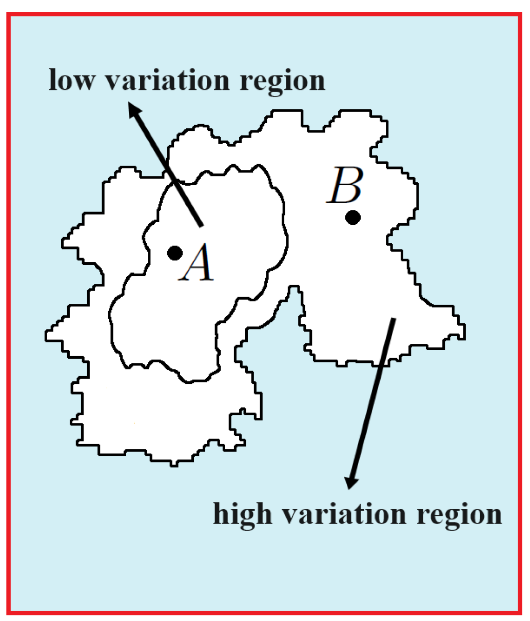
In the second method, we utilize the rate of change in the temporal approximation to divide the missing region into low-variation and high-variation sub-regions (see Figure 1). This approach aims to guide the Poisson blending technique for non-homogeneous regions with different variations. Farm fields are good examples for applying this model, as cropland in a growing season has high temporal variation, while buildings and roads have lower variation. In our method, we can change the relative weight of spatial and temporal components based on the temporal variation at each point. The temporal approximation can be weighted more for the points with less temporal variation (e.g., buildings in farm fields), while the spatial component can be weighted higher when the areas have higher temporal variations (e.g., cropland).

Figure 1.
Two points in different zones (sub-regions): A is a point in a low-variation region and B is a point in a high-variation region.
We conducted thorough testing to assess our proposed methods’ effectiveness. During this evaluation, we compared the outcomes of our new methods with those of the conventional temporal and spatial approximation techniques. Our new spatial–temporal approximations exhibit greater accuracy and versatility than the standard temporal and spatial approximation methods. For instance, our methods resulted in an average increase in accuracy of 190% and 130% compared to spatial and temporal approximations in all case studies. Importantly, these advancements were achieved while maintaining the same complexity as conventional methods (linear in the number of pixels in the region of interest).
In summary, our main contribution is a new variational model for the spatial–temporal approximation of time-varying satellite imagery, which addresses missing or masked data caused by clouds and shadows. Based on this model, we developed two novel methods that outperform conventional techniques in accuracy and versatility while maintaining the same complexity.
The structure of this paper is as follows: We begin with an overview of the existing literature and works related to our method in Section 2. In Section 3, we introduce the concept of our methods, which include a spatial–temporal approximation based on Poisson image blending and a more general spatial–temporal approximation by involving the variations in each pixel inside the desired region. The evaluation of our method and its performance is discussed in Section 4. Finally, we conclude the paper in Section 5.
2. Related Works
There are various types of methods to reconstruct a region in an image in a set of satellite images. These methods approximate the desired region using spatial and/or temporal information. First, in Section 2.1, we provide an application of such approximation methods. Then, we provide different categories of approximation methods.
2.1. Time-Varying Remote Sensing Imaging Applications
Various fields can benefit from the reconstruction of a region. One such field is vegetation monitoring. For vegetation monitoring applications, spatial–temporal reconstruction techniques play a critical role in enhancing data quality and analysis capabilities. For example, Meng et al. [6] generated Normalized Difference Vegetation Index (NDVI) data with high spatial and temporal resolutions for crop biomass estimation. This approach, enabled by spatial–temporal reconstruction, allowed for more accurate estimates of crop yield and productivity. By using spatial–temporal reconstruction to fill data gaps, Atzberger et al. [7] employed an approach named unmixing to obtain crop-specific time profiles of the NDVI. By incorporating data generated via spatial–temporal reconstruction, Yang et al. [8] investigated the influence of natural and anthropogenic factors on vegetation changes through structural equation modeling. In another paper, Jiang et al. [9] analyzed the spatial patterns of and dynamic changes in vegetation greenness from 2001 to 2020 in Tibet, China. Spatial–temporal reconstruction techniques allowed them to fill missing data gaps, leading to a more accurate and complete picture of vegetation trends over time.
There are also plenty of works for land cover mapping applications that use spatial–temporal reconstruction techniques to provide enhanced insight and accuracy. Ali et al. [10] analyzed hyper-temporal NDVI imagery by employing spatial–temporal reconstruction to effectively map land cover gradients. This approach captures the dynamic changes in land cover over time, leading to more comprehensive mapping results. Also, Faizal et al. [11] applied NDVI transformation to Sentinel-2A imagery, combined with spatial–temporal reconstruction, to accurately map mangrove conditions.
2.2. Inpainting and Interpolation
One approach to reconstructing satellite images involves inpainting, which fills in missing regions using information from the surrounding pixels. For example, Cheng et al. [12] developed a method using a multichannel nonlocal total variation model that takes advantage of spatial coherence between different spectral bands to achieve this reconstruction. As another technique, Shen et al. [13] proposed an algorithm that combines statistical priors with image data to handle striping and sensor malfunction. Furthermore, Hu et al. [14] proposed an inpainting method that utilizes structured low-rank matrix approximation. The technique reconstructs missing regions in remote sensing images, especially in areas that have repetitive patterns. Armani et al. [15] provided an inpainting algorithm based on partial differential equations (PDEs) for compressing hyperspectral images; this approach inpaints the images spatially by a Laplacian equation.
Usually, inpainting methods use the information in the surrounding pixels. However, some inpainting methods use another image to fill the unknown region by applying a fusion method. Pérez et al. [3] presented Poisson Image Editing, which seamlessly clones another image to fill the unknown region. The method uses the Poisson equation to create smooth transitions between the two images. An extended version of this method that introduces user guidance mechanisms was presented by Di Martino et al. [4]. This method allows for interactive control over the inpainting process, enabling users to steer the reconstruction toward desired outcomes. Later, Farbman et al. [16] introduced the edge-preserving decomposition method, which focuses on preserving fine details and sharp edges during inpainting. The Poisson Matting method introduced by Sun et al. [17] is another method for handling some scenarios involving object boundaries and transparency. It uses a trivariate Poisson equation to seamlessly integrate foreground objects onto new backgrounds.
One approach to managing missing data in spatial reconstruction is the use of interpolation techniques. These methods estimate missing values by looking at the values of nearby known pixels or points. Interpolation techniques use spatial and/or temporal relationships within the data to fill in the gaps and reconstruct the missing information smoothly and consistently. One such method called GP-GAN, introduced by Wu et al. [18], uses generative adversarial networks (GANs) and Gaussian processes (GPs) to produce high-resolution image blends that look realistic. This method works by learning the statistical distributions of the data, allowing it to accurately fill in missing regions. Tanaka et al. [19] proposed a modified Poisson problem as a closed-form solution for seamless image cloning. The method interpolates missing regions, ensuring smooth transitions and seamless integration with the surrounding data.
In a recent work, Hu et al. [20] proposed an automatic algorithm to remove clouds from Landsat satellite images. Their method uses built-in cloud mask data and considers factors like image similarity to find the best cloud-free images for patching. It then fills cloudy areas with clear land pixels from these reference images and blends the patched area seamlessly. Tested on a large dataset, the method shows promise for creating a cloud-free Landsat time series for land cover studies.
The main drawback of inpainting or interpolation is that using these methods results in a loss of information in the temporal dimension. In other words, these methods fill the unknown region with surrounding pixels’ information.
2.3. Time Series
Another category for the reconstruction of a region is using a time-series approximation. For example, the study in [21] investigated vegetation changes in Xinjiang from 2001 to 2020 by analyzing time-series MOD13Q1 NDVI data and MCD12Q1 vegetation-type data and focusing on the relationship between vegetation-type and NDVI changes. In another work, Zhou et al. [22] proposed a deep learning approach utilizing Long Short-Term Memory (LSTM) networks for reconstructing missing data in Landsat images. Jordi et al. in [23] introduced a method based on the Discrete Cosine Transform and Partial Least Squares (DCT-PLS) for reconstructing cloud-covered areas in satellite image time series. It leverages temporal information to predict missing data points within the series.
When we use time-series approximation methods, one significant downside is that we lose information in the spatial dimension. In other words, these methods fill in the unknown regions by using only the information from the corresponding pixels in temporally neighboring images.
2.4. Fusion and Mixing of Low-Resolution and High-Resolution Images
Several spatial–temporal reconstruction methods employ data fusion techniques, where information from multiple satellite images with diverse spatial and temporal resolutions is combined to produce a high-quality output. The data fusion method developed by Liu et al. [24] can account for variations in the relationships between low- and high-resolution data. It offers improved accuracy but can be computationally demanding. The generalized linear spectral mixing model introduced by Zhou et al. [25] is a model-driven approach that captures the spectral and temporal features of land cover types. It handles mixed pixels but needs accurate prior information. In addition, He et al. [26] proposed a method to fuse multi-source remote sensing images for abandoned land detection. This method requires careful selection and processing of diverse data sources for optimal results.
As another approach to improving spatial–temporal approximation, some studies have suggested combining two sets of satellite images with different scales, one with a low resolution and another with a high resolution. For example, Rao et al. [27] introduced an NDVI Linear Mixing Growth Model (NDVI-LMGM), an unmixing-based method for blending MODIS NDVI time-series data and Landsat TM/ETM+ images. In another work, Xue et al. [28] used the precise registration between heterogeneous remote sensing images to accommodate differences in the sensor type, resolution, and imaging conditions. Also, the proposed method in [25] provided a method for fusing hyperspectral images (HSIs) with low temporal and spatial resolutions and high-resolution multispectral images (MSIs). Meng et al. [6] proposed a Spatial and Temporal Adaptive Vegetation index Fusion Model (STAVFM) that combines the high spatial resolution of HJ-1 CCD images with the high temporal resolution of MODIS, overcoming the limitations of each data source.
To use methods that mix low-resolution and high-resolution images and utilize fusion, data from two different satellites are needed, which is problematic when one has only a set of images from one satellite. Also, some of these methods use both temporal and spatial data, and they need more attention to the consistency of the data from different sensors or satellites.
2.5. Machine Learning and Deep Learning Approach
Recently, some spatial–temporal reconstruction techniques have used machine learning methods to fill in the unknown region of one image in a set of satellite images. For instance, Shen et al. [29] provided a method to monitor complex human–nature interactions using a bi-directional strategy with the Random Forest algorithm to reveal the impact of policy dynamics on land-use conversion. Also, Chen et al. in [30] proposed a spatial–temporal neural network for remote sensing image change detection, incorporating a mechanism to model spatial–temporal relationships between co-registered images taken at different times. Another work by Chen et al. [31] introduced a learning-based spatiotemporal fusion method called Multiscale Attention-Aware Two-Stream Convolutional Neural Networks (MACNN) for producing fine-scale remote sensing images by blending two types of satellite images.
As another approach, many spatial–temporal reconstruction techniques use deep learning methods to improve their accuracy. They achieve this by utilizing deep neural networks to learn the complex relationships between spatial and temporal information within satellite images. This enables them to reconstruct regions that are missing or degraded with acceptable accuracy and detail. For example, Shao et al. [32] created a model for urban remote sensing that captures the interplay between spatial, temporal, and spectral information. The improved generative adversarial network presented by Zhu et al. [33] handles the challenge of remote sensing image super-resolution reconstruction. It uses the adversarial nature of these types of networks to produce high-resolution images from lower-resolution ones. Jiang et al. [34] proposed a deep learning method to reconstruct remote sensing images with cloud cover. Also, this approach uses deep learning to remove clouds and recover image content. Finally, transformer models were recently applied to remote sensing image change detection by Chen et al. [35], demonstrating promising results in identifying subtle changes over time. In another work, Chen et al. [36] applied a deep learning model for optical remote sensing image cloud processing. In recent research [37], Long et al. proposed a new method for removing clouds from satellite images using a bishift network (BSN) that tackles the issue of time differences between images by using two steps. First, it adjusts the images using moment matching and deep style transfer to make them more alike. Then, an improved version of Shift-Net removes the clouds.
Despite these successes, training deep learning and machine learning models requires extensive computational power and large datasets, making them unsuitable for small datasets.
2.6. Choice of Method
Since there are many applications for the reconstruction of an unknown region by spatial–temporal approximation, the choice of method depends on various factors, like the extent of missing data, image quality, computational resources, consistency among available data, and the size of the dataset. Therefore, the method introduced in this paper is going to overcome the mentioned issues in other methods with a spatial–temporal structure and a variational version thereof.
3. Methodology
Remote sensing with time-varying satellite imagery has revolutionized our ability to monitor the Earth’s surface. However, the presence of clouds and their shadows in satellite images poses a significant challenge, as they can obscure critical information about the Earth’s surface. In this section, we introduce our approach to addressing this issue and provide two spatial–temporal approximations of satellite images.
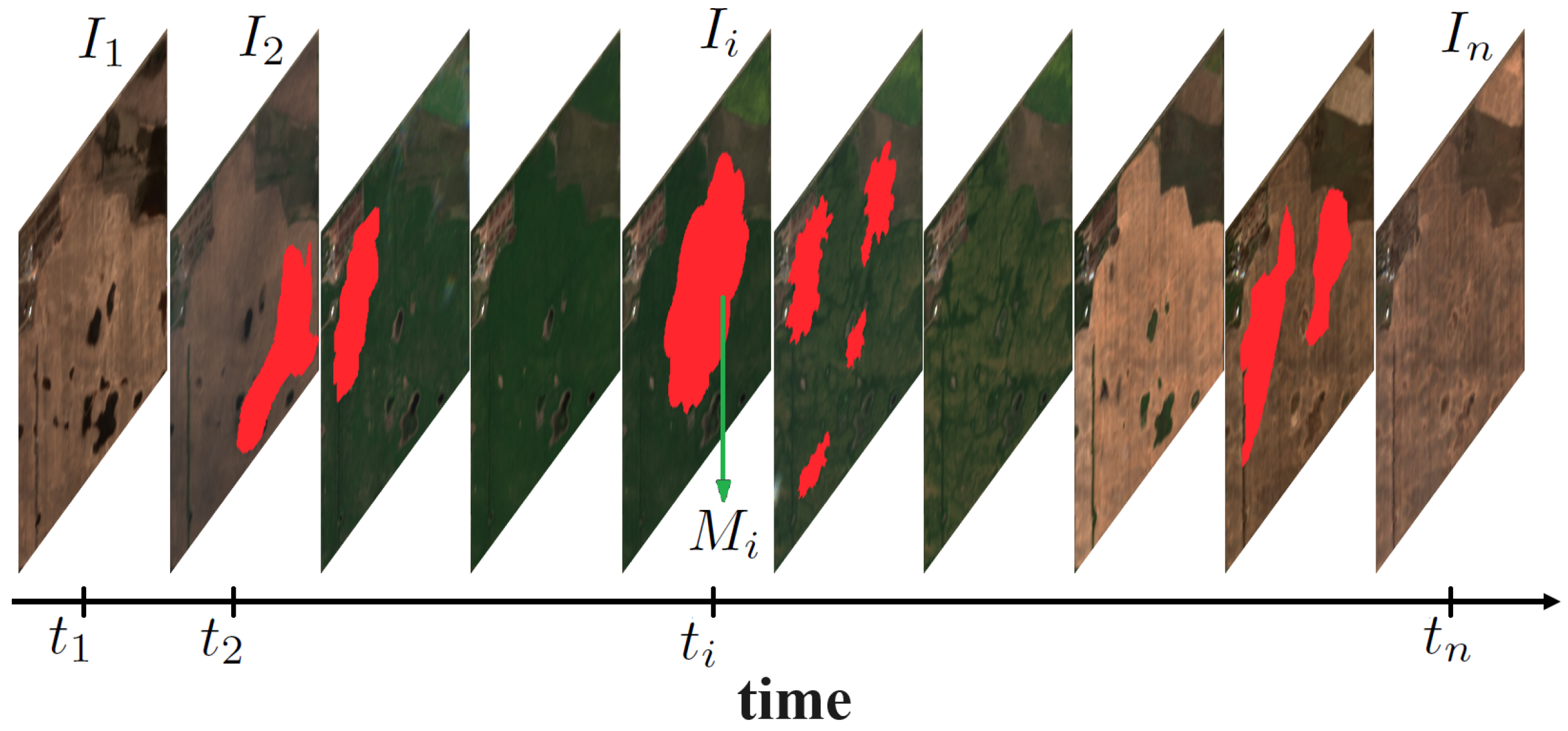
Our method begins with a set of satellite images captured in a time period, with the image set denoted by , each corresponding to a specific time . As shown in Figure 2, these images come with their respective masks resulting from cloud and shadow detection methods [38,39,40,41,42].
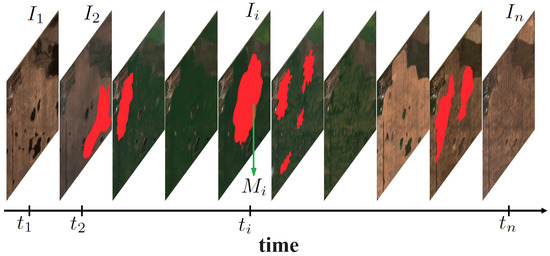
Figure 2.
A set of images with their corresponding times and masks (red regions).
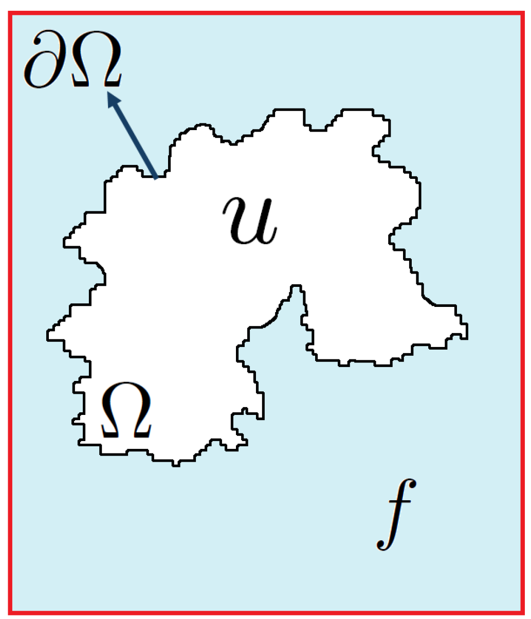
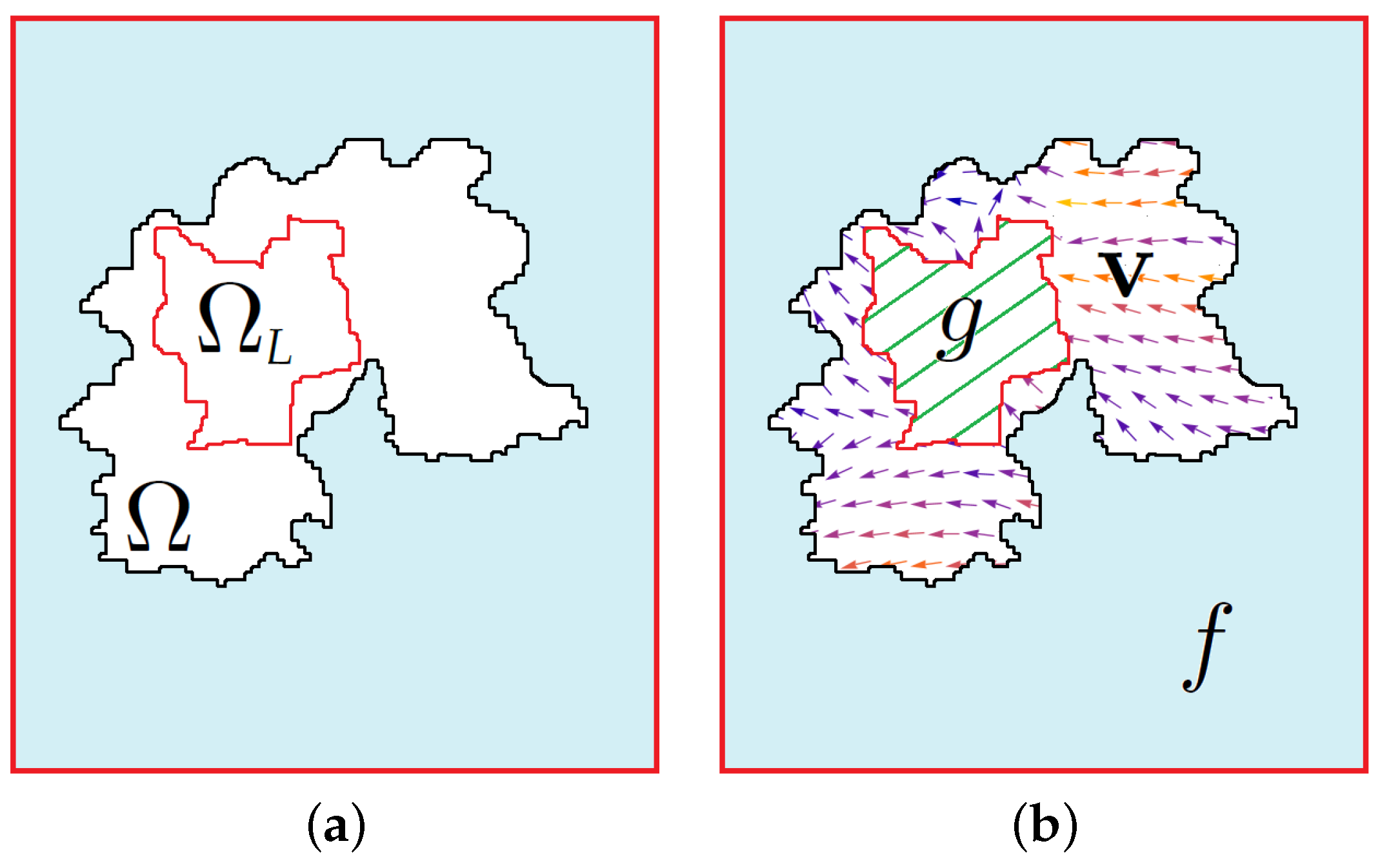
For the target image , in the target time , the pixels under are removed, and the resulting region is denoted by (see Figure 3). Our goal is to approximate and reconstruct f in . As demonstrated in Figure 3, we denote the boundary of by and the approximating function by u. Our method for constructing u relies on both temporal and spatial approximations in .
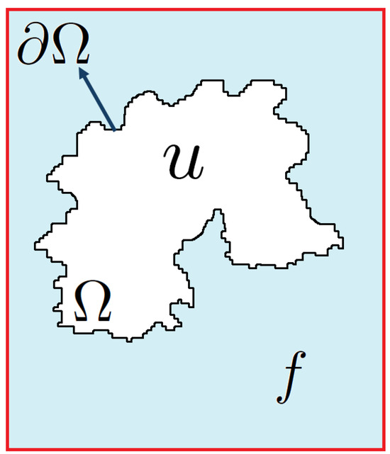
Figure 3.
The target image with a masked region and the approximating function u.
There are different methods to reconstruct an image within a specific region, depending on the available data. These methods can be categorized into three types: temporal approximation (i.e., using a time series of images), spatial approximation (i.e., using the available data in ), and finally, spatial–temporal approximation (i.e., a combination of temporal and spatial approximations). Our proposed method falls under the spatial–temporal category, utilizing both temporal and spatial approximations in the final model.
In the following, we will discuss each of these methods individually.
3.1. Temporal Approximation
One strategy to approximate the image inside is to use a set of univariate approximations for all pixels within the region as a temporal approximation.
For the temporal approximation component of our final model, we compute a pixel-wise approximation of the image, denoted by . This approximation relies on finding an approximation of the image in using some of the previous and next available images in the sequence of images.
Various techniques can be employed to estimate a time-based image using a given set of images. Some of these techniques include time-series techniques such as the simple mean, weighted mean, weighted moving average (WMA) [43], and autoregressive integrated moving average (ARIMA) [44]. Some general techniques can also be used, including nearest neighbor (NN) and k-nearest neighbor (ANN) [45], weighted nearest neighbor (WNN) [46], moving least squares (MLS) [47], local least squares (LLS) [48], inverse distance weighting (IDW) [47], and finally, regression [49], and radial basis function (RBF) methods [50].
An efficient method would be to minimize the sum of squared errors for the given time periods. Using this method, a wide range of functions can be used as an approximating function, whether they have a linear or nonlinear format based on their parameters.
Let be the set of all univariate parametric functions of parameters ,⋯, with a predefined form. In this approximation, for every fixed pixel , we seek a univariate temporal function to approximate for , and we have
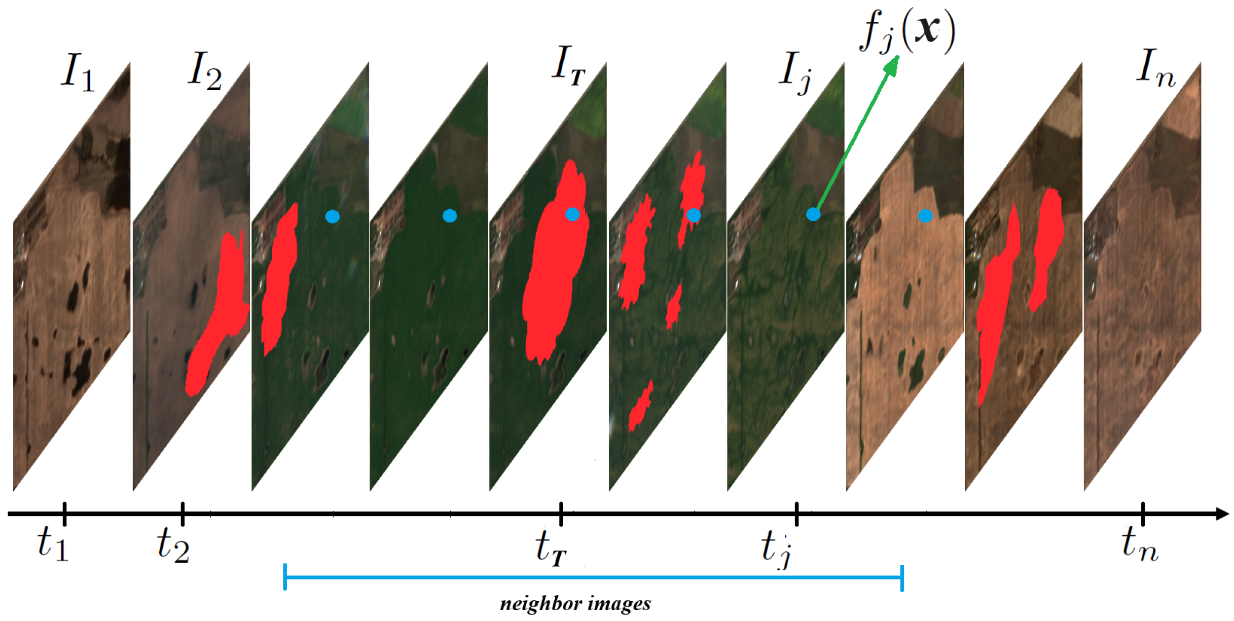
where is the set of all possible neighbor indexes to the target time with a distance of , and is the value of the pixel in image , (see Figure 4).

Figure 4.
The different values for a pixel (blue point) in temporally neighboring images.
Consider to be a linear function in its parameters (i.e., for a set of linearly independent functions ) that provides a linear least-squares problem, while a nonlinear form of results in a nonlinear least-squares problem.
In Equation (1), if we choose the neighborhood, , as the set of indexes of all images, it provides us with a global approximation, while, if we restrict it to some limited number of images around the target time , it gives us a local approximation.
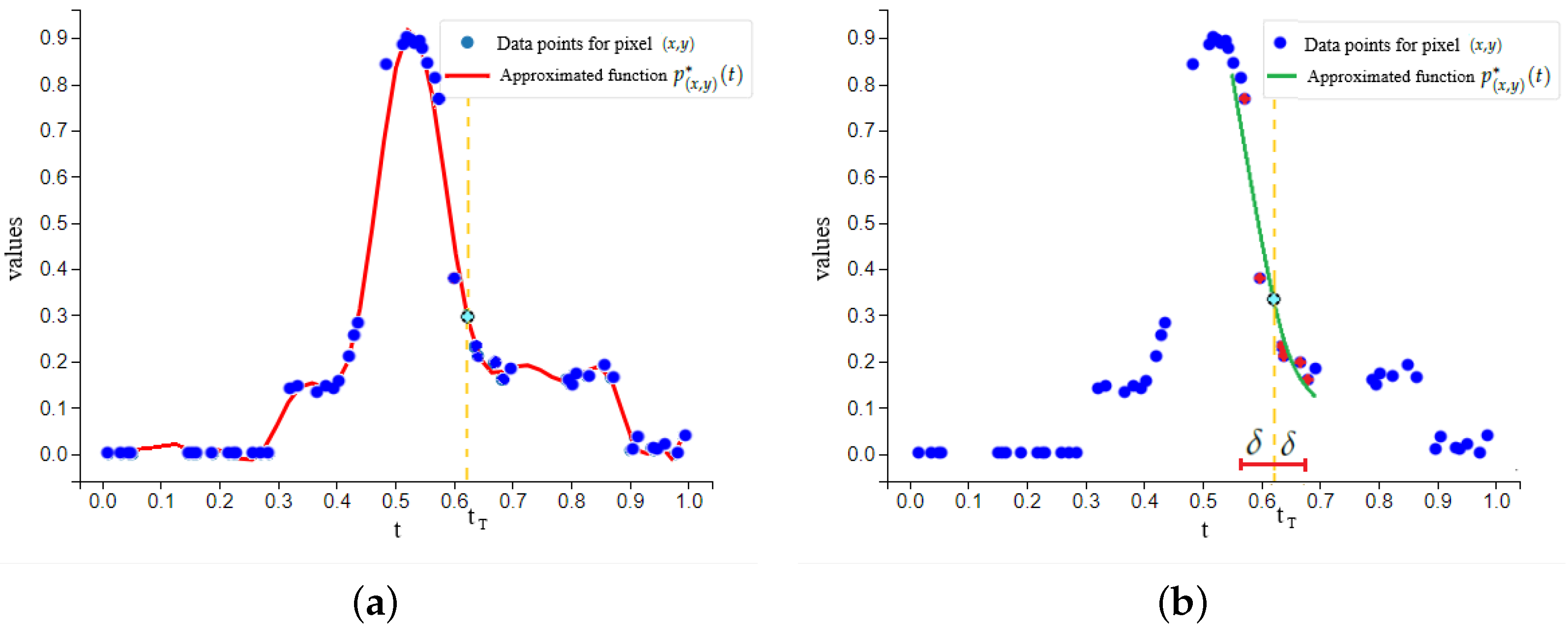
An example of such an approximation for a pixel can be seen in Figure 5. In this figure, Figure 5a shows a global approximation, and Figure 5b is a local approximation.
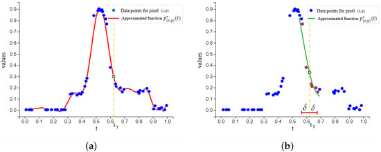
Figure 5.
Pixel-wise approximations for a pixel. (a) The approximating point (green point) is calculated based on a global approximation. (b) The approximating point (green point) is calculated based on a local approximation using nearby points (red points).
By adding a weight to each point, we can control its impact on the resulting approximating function. Therefore, we consider a weighted least-squares problem:
where values are non-negative weights such that the closer point to the target time has the larger value for the corresponding weight. Thus, the weights are the values of a decreasing function of the distance of the time t from the target time (i.e., , where h is a decreasing function). For a global approximation, all weights are non-zero, while for a local approximation, the weights are zero for points that are far away from the target time according to a given threshold value.
The function form, the target time, and the length of the time period must be determined for the temporal approximation. For example, a common choice for the function for the global approximation of the NDVI is the asymmetric double-sigmoid function [51,52,53]:
where , and d are different real parameters.
In a single growing season, the candidate function is expected to behave like a skewed bell-shaped curve (i.e., a smooth function with a single unimodal maximum). This is because the NDVI value increases before the peak time and decreases after the peak but not necessarily in a symmetric fashion. Therefore, the asymmetric double-sigmoid function is a suitable candidate for the global approximation of the NDVI time series. A comparison between different function forms for the NDVI can be found in [54].
Generally, after finding for every pixel inside , the temporal approximation g in the target time is
for every pixel (i.e., g represents the temporal image ). Therefore, g is used for a temporal approximation of the missing part of in the target image:
For the rest of the image, u is identical to f.
The temporal approximation of in represents our initial attempt to restore the image’s missing data by considering only temporal changes (see Figure 6).

Figure 6.
Filling in the missing region with the temporal approximating function g.
A temporal approximation offers the advantage of capturing temporal trends and changes within the region , making it particularly valuable not only for approximating the missing data but also for understanding the dynamics of the underlying processes and monitoring variations over time. This method is well suited for scenarios where temporal changes are the primary focus, providing insights into trends and patterns. However, its exclusive use of temporal approximation comes with notable drawbacks. It disregards spatial details, leading to a loss of resolution and the potential misrepresentation of complex spatial features in dynamic regions. Also, the accuracy of the temporal approximation heavily depends on the revisit time of satellite images (and also the possibility of completely cloudy days).
3.2. Spatial Approximation
Another approach to approximating the image inside is to fill the desired region by using a smooth approximation of the available data outside of as a spatial approximation. One such approximation uses the Laplace equation with boundary conditions [55,56]:
where is the Laplacian operator: i.e., for a 2D image, we have . The basic idea is that the image inside is reconstructed smoothly by a harmonic function based on the values on . There are different numerical methods to solve Equation (5), including the finite element method [57], the finite difference method [58], the Adomian decomposition method [59], and geometrical transformation [60]. Therefore, by solving Equation (5), the approximating function is computed for the desired region (see Figure 7).
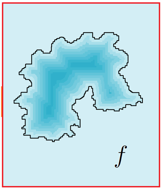
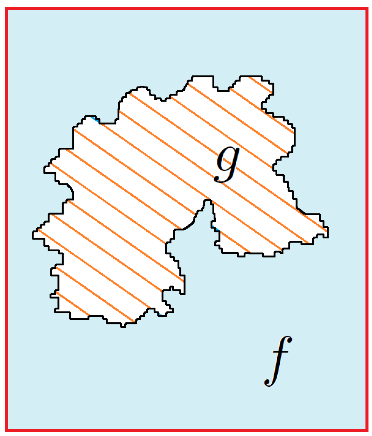
Figure 7.
Filling in the missing region by using the Laplacian equation. The region is mostly affected by its boundary values. The closer the point to the boundary, the closer the value of the approximating function to it.
This method is usually good when the image has homogeneous behavior, independent of the temporal behavior, in a spatial neighborhood of containing this region. As a result, it is not able to accurately represent the dynamic nature of non-homogeneous regions. For this kind of region, it is better to employ spatial–temporal approximations.
3.3. Spatial–Temporal Approximation
For the third approach, we combine temporal and spatial approximations to enhance the approximation further. As previously stated, a spatial approximation cannot provide an accurate representation of the ever-changing nature of some regions, and it does not account for temporal variations. Conversely, a temporal approximation overlooks spatial intricacies, resulting in possible misinterpretation of complex spatial features.
We need a method that overcomes the issues mentioned above, and it should consider both the spatial and temporal features of the problem. The challenge is to find a model that contains both spatial and temporal aspects of the time-varying phenomena. A simple weighted combination between temporal and spatial approximations cannot properly capture the interdependency between them.
One approach is to combine two images, each chosen for a specific reason, to reconstruct the image in the desired region . For example, the Poisson image blending method [3] is a very effective method for seamless image cloning. This method works by filling a specified region with content from the source image and then smoothing out the resulting image to better match the target image. Overall, it is a spatial method that is useful for creating composite images that look natural and cohesive. We extend this method for the purpose of spatial–temporal modeling.
3.4. Poisson Image Blending
Poisson image blending [3,4] is a widely used and effective technique in computer vision and image processing for seamlessly blending or transferring the content of one image to another while preserving the target image’s structure and texture (see Figure 8). The method aims to find a new image corresponding to the function u, whose gradient closely resembles a desired vector field within a specified region while adhering to a given target image outside of . This optimization process involves minimizing a specific energy functional, represented by
with the boundary condition over .
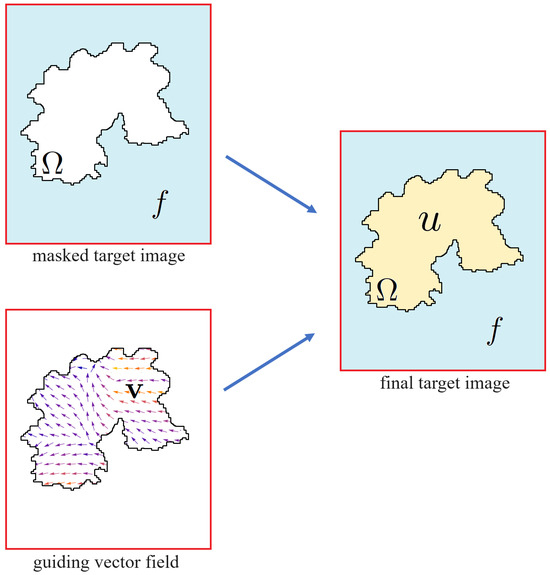
Figure 8.
Blending the guiding vector field with the target image.
In Equation (6), u represents the approximating function, and is the desired vector field, named the guiding vector field over . Also, ∇ is the gradient operator of images (i.e., for 2D images, ), and . Here, denotes the Euclidean norm.
The main reason for using the guiding vector field is that it guides the pixel value transfer from one image to another image by minimizing artifacts and ensuring smooth, coherent results by controlling the diffusion direction.
The aim of minimizing the energy functional (6) is to find an approximating function u whose gradients within the region are similar to those of the target image with the corresponding vector field . The vector field is conservative if it is the gradient of another function s. The similarity between the approximating function u and the vector field ensures a smooth blend and consistent texture. The minimization process is typically conducted using variational calculus, which leads to the derivation of the Euler–Lagrange equation that characterizes the minimizer of the functional.
The corresponding Euler–Lagrange equation for the energy functional (6) with the boundary condition is as follows:
where is the Laplacian operator, and div is the divergence operator over a vector field (i.e., for a 2D vector field, we have ). This equation can be solved by the discrete Poisson solver method presented in [3].
3.5. Spatial–Temporal Poisson Approximation
As already mentioned, the Poisson image blending method is a technique that allows us to blend two static images. Our model is based on the fact that the temporal approximation g is better used for guiding the spatial reconstruction. Therefore, we use as the guiding vector field but the available spatial values as the target image.
This means that the guiding vector field comes from the temporal approximation g, and consequently, the energy functional is defined by
with the boundary condition over .
In Equation (8), u and g represent the desired spatial–temporal and temporal approximations, respectively.
The corresponding Euler–Lagrange equation for this system is an equivalence equation with the following format:
where is the Laplacian operator.
We first find g, the temporal approximation of the target image in the region . Then, we use Equation (9). To find u, this equation requires that the Laplacian of the approximated image u match the Laplacian of the temporal approximation g within the region , preserving local variations and structures:
where f is the function of the target image , g is the initial approximation obtained as the temporal approximation of the unknown function, is the boundary of , and u is the desired spatial–temporal approximation.
So, our first algorithm aims to provide a spatial–temporal approximation for a set of satellite images. Given a set of images , corresponding masks , and a cloudy target image , Algorithm 1 results in an approximated image by using our spatial–temporal Poisson approximation method.
| Algorithm 1: Spatial–temporal Poisson approximation |
|
3.6. Variational-Based Region Restoration
When using the spatial–temporal approximation derived from Equation (8), the impact of every point within the region is considered equal. However, different points may have different scales of variation in time. For example, consider a farm field that has some roads and buildings in the field side by side with cropland. It is expected to see large changes in the NDVI of the cropland but no changes or small changes in the roads and buildings in a period of time. Hence, to better capture this inhomogeneity, we introduce a variation-based model that is a generalization of the spatial–temporal Poisson approximation method. In this model, in addition to the guiding vector field to control the variation in the approximated function, we use a guiding function s to control the value of the approximation.
The model is formulated as an energy functional, denoted by , defined over a specified region . The functional is expressed as
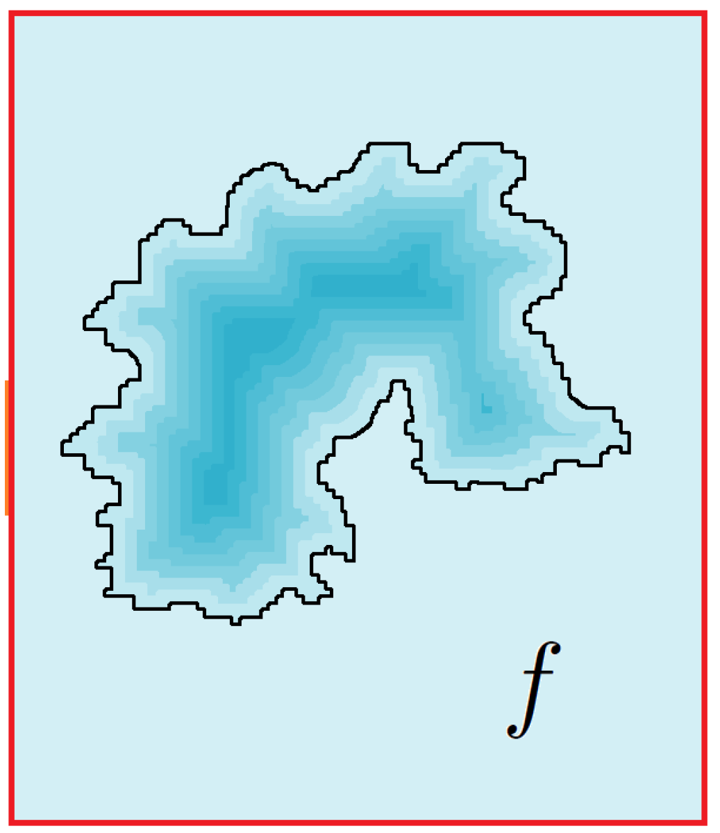
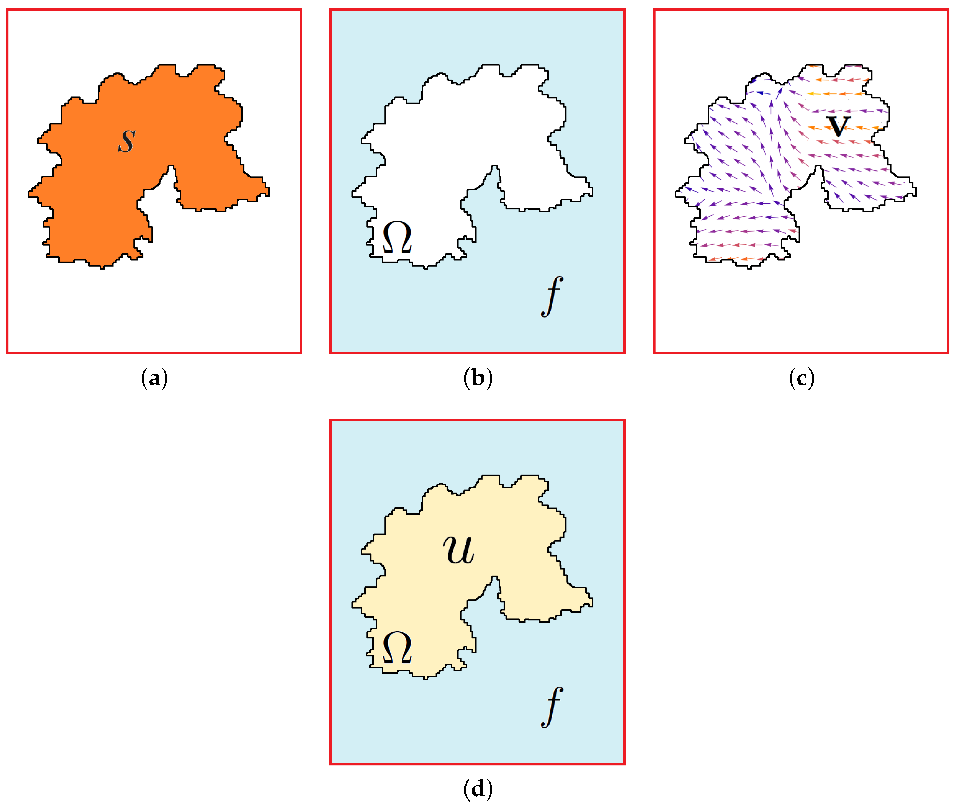
with the boundary condition over . In Equation (11), u represents the approximating image function, and ∇ is the spatial gradient operator (see Figure 9).
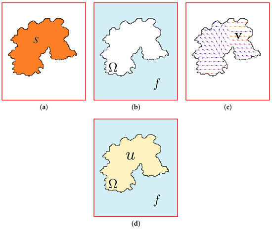
Figure 9.
The elements of the variational-based region reconstruction model. Three elements ((a) the guiding image s, (b) the target image, and (c) the guiding vector field ) are used to find the final reconstructed image (d).
In Equation (11), the term captures the guiding vector field control aspect by penalizing the difference between the gradient of the reconstructed image and the scaled version of the guiding vector field , weighted by the parameter . The term incorporates the guiding function control aspect, penalizing the difference between the approximating image function and a scaled version of the guiding function s. The method seeks to find the optimal reconstruction by minimizing this combined energy functional, effectively integrating the effect of both the guiding function s and the guiding vector field for improved region reconstruction in the target image. Also, the approximating function u is equivalent to the target function f outside of , and generally, , , and are non-negative functions over .
The Euler–Lagrange equation for the given functional is obtained by finding the stationary point of the functional for the function u. The Euler–Lagrange equation for (11) is as follows:
where , ∇, and div are the gradient operator, the divergence operator, and the Laplacian operator, respectively. Also, all matrix multiplications are element-wise multiplications (Hadamard multiplication): i.e., each element in the resulting matrix is obtained by multiplying the corresponding elements of the input matrices.
Solving Equation (12) provides an image that captures the effect of both the guiding function and the guiding vector field.
While Equation (12) is a spatial method, the guiding function s and the guiding vector field can be used to include the temporal aspects of our spatial–temporal model. Therefore, we introduce a new spatial–temporal approximation based on this method that captures both spatial and temporal features.
3.7. Variational-Based Spatial–Temporal Approximation
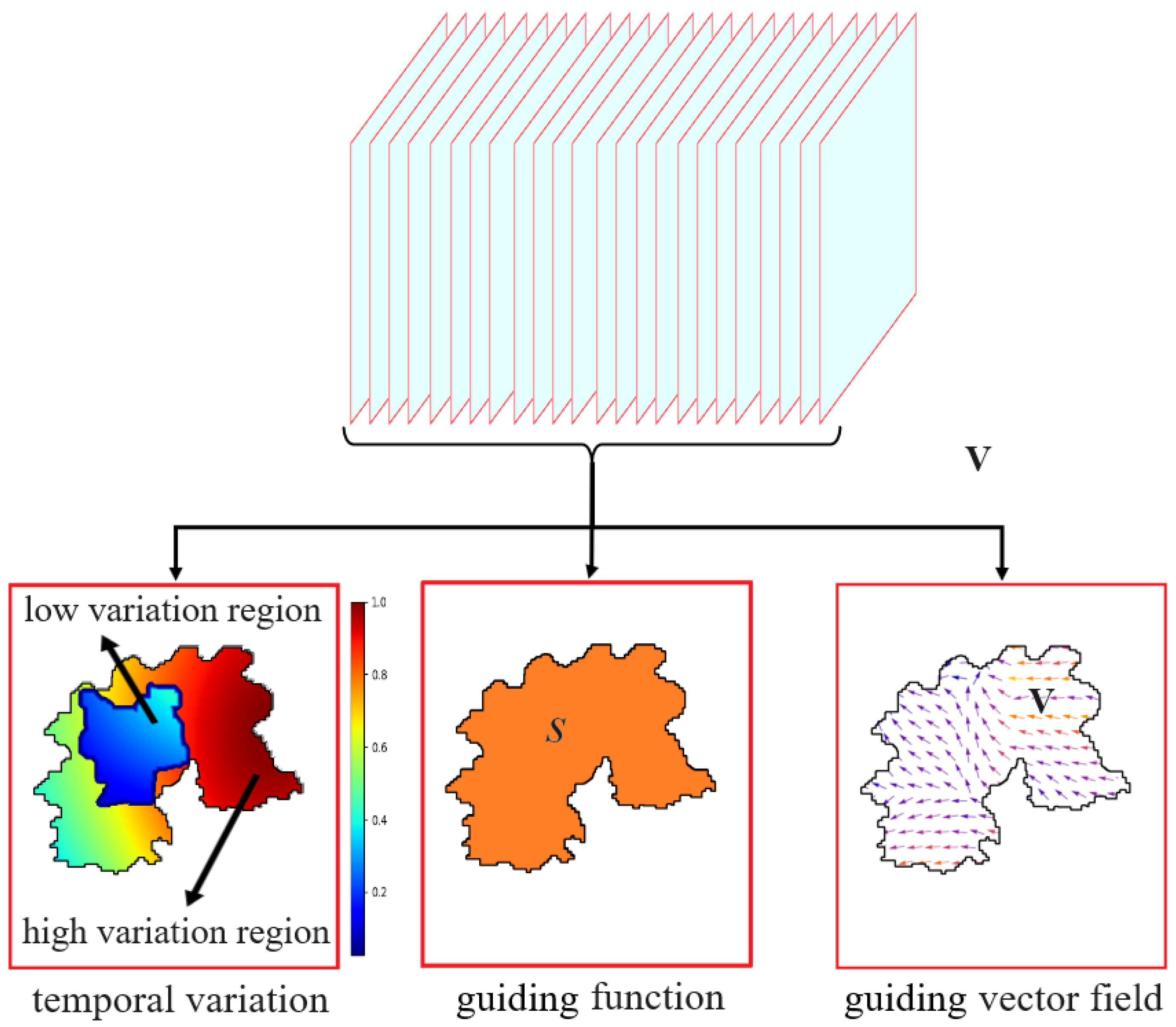
Similar to spatial–temporal Poisson approximation, we seek a new approximation that captures both the spatial and temporal aspects of the image inside the region . In the variational-based region restoration method (12), we have two parameters, s and , as the guiding function and guiding vector field, respectively, resulting in an approximation that can be controlled based on temporal variation in the image set. This generally means that the guiding function s and guiding vector field can both be computed from temporal approximations over the given time period (see Figure 10).
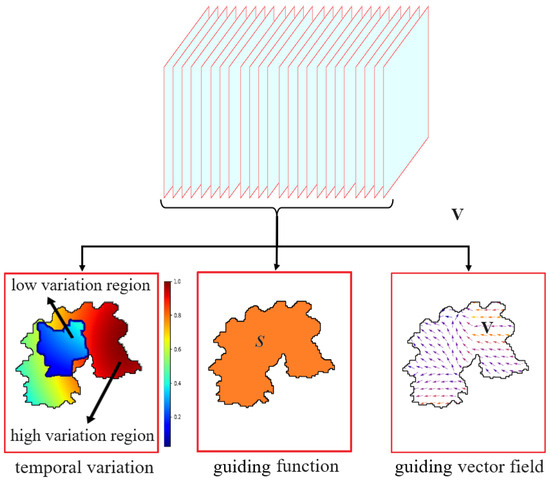
Figure 10.
The temporal variation, guiding function, and guiding vector field. The temporal variation related to all pixels in is provided in the left image. The color blend represents the value of the variation in pixels. Specifically, it is a color blend from blue (low-variation) to red (high-variation).
Thus, first, we find a temporal approximation g of the target image in . We use this initial approximation as the guiding function (i.e., ). One option for the guiding vector field is to use the gradient of the guiding function rather than finding another temporal approximation (i.e., ). Therefore, the following energy functional should be minimized over the desired region :
with the boundary condition over .
The Euler–Lagrange equation corresponding to Equation (13) is given by
where g and u are the temporal and the spatial–temporal approximating functions.
Our variational model allows for customizing the parameter functions and to better capture non-uniform variations across . These functions can be computed based on the temporal variation during the given time period. The spatial aspect and temporal aspect are directly correlated to and , respectively. When the temporal variation at is low, is a good approximation, and this can be captured by a larger and a smaller . On the other hand, if the temporal variation at is high, the approximation obtained from the guided vector field is more reliable. This can be captured by a larger and a smaller . Consider Figure 1. For point A, we have lower variation, a bigger , and a smaller . For point B, we have higher variation, a smaller , and a bigger .
There are different ways to measure the temporal variation in a specific pixel in a set of satellite images over a time period. One way is to use spectral variation, which measures the changes in the reflectance of light from a material as a function of wavelength [61]. The two main methods for the computation of the spectral variation types are statistical measures and image differencing. In the first method, statistical measures like the mean, standard deviation, minimum–maximum, and coefficient of variation are used to capture the variation. In the second approach, the variation is computed using image differencing that calculates the difference images between consecutive images or between specific time periods.
One simple and efficient spectral variation method is to use the pixel-wise coefficient of variation for the given period. For every point , the coefficient of variation is given by [62]
where v is the temporal variation image; and are the mean and standard deviation of the pixel during the given period, respectively. Note that and are also functions of time. A higher indicates a higher relative variability of point , while a lower indicates a lower relative variability.
Our variational model in Equation (14) is very general and flexible. For example, Equation (14) for and is equivalent to Equation (4), and this means using the temporal approximation g as the approximating function u on . For , , and , Equation (14) is equivalent to the Laplacian Equation (5), and , , and convert Equation (14) to our Poisson image blending Equation (10). Also, the modified Poisson problem discussed in [19] is a specific version of Equation (14) for , , and , where is a small positive number. Finally, for and , our model reduces to the total variation (TV) model [55].
3.8. Binarized-Variation-Based Spatial–Temporal Approximation
A simple but useful and novel special case of our general model is the case where the region is divided into two high-variation and low-variation regions. This method is a specific case of the variational-based spatial–temporal approximation method introduced in Section 3.7. Farmland is a good example for applying this model, as cropland in a growing season is a high-variation region, but the buildings in the farm belong to the low-variation region.
Similar to other methods, the first step involves removing the cloudy part from the target image based on the provided cloud and shadow masks. Then, we compute the temporal variation v in the images in a given period and a new mask based on the temporal variation information. This mask represents the region with low variation. To find this mask, we use a threshold . Therefore, if , belongs to the low-variation region, and if , belongs to the high-variation region. This thresholding provides us with a subset of the region, (see Figure 11), representing the low-variation region.
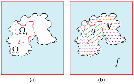
Figure 11.
The guiding elements and their corresponding regions. (a) The low-variation region. (b) The guiding components.
Considering Equation (13), the basic idea is to rely mostly on g for the low-variation region and mostly on for the high-variation region. Therefore, we consider inside and outside of the region. Additionally, we set inside and outside of the region. So, we have a convex combination of two parts, and the equation is converted to a new equation.
In this equation, we clone the temporal approximation g into the target image based on the new mask . Then, we use the following equation to find the spatial–temporal approximation u:
So, the binarized-variation-based spatial-temporal approximation method is based on Algorithm 2.
| Algorithm 2: Binarized-variation-based spatial–temporal approximation |
|
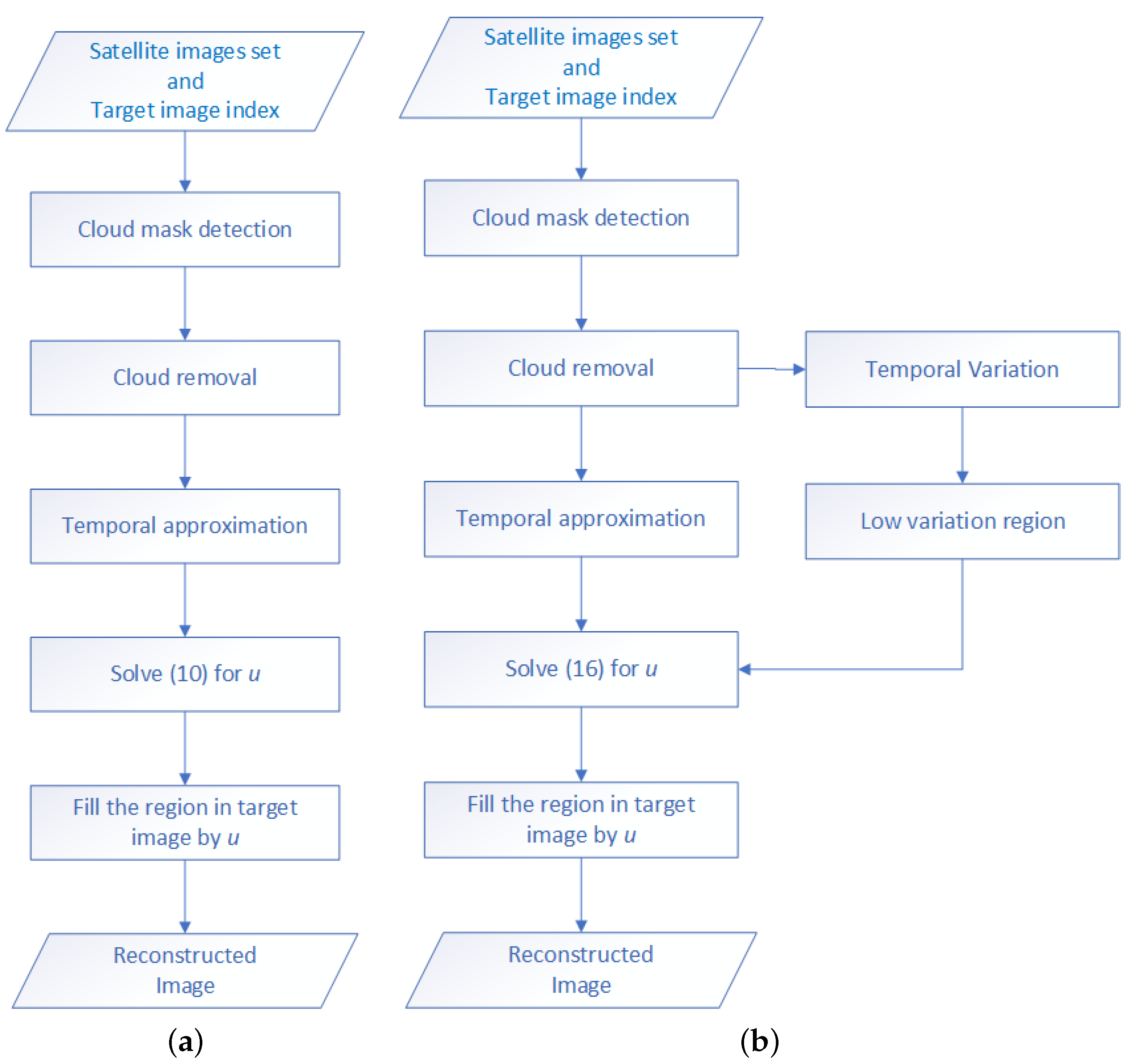
To find , we need to find a suitable threshold , so we propose a spatial analysis over the temporal variation v to find this threshold. Using this analysis, we compare the pixel’s variation with its spatial neighbors’ using statistics like the local standard deviation, the coefficient of variation, or Moran’s I [63], which is a measure that shows the degree of spatial dependence or clustering among observations. In Figure 12, flowcharts of our methods are provided.
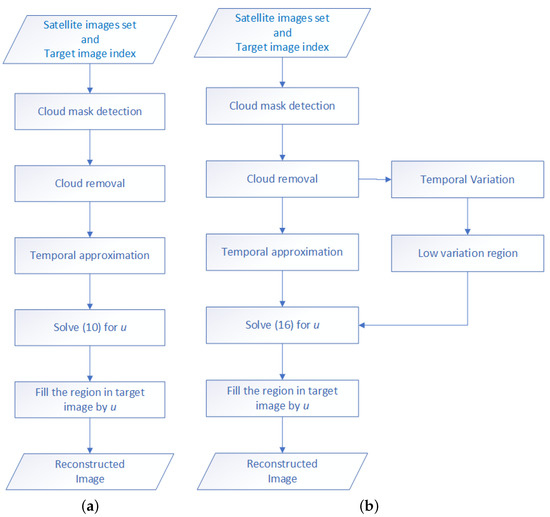
Figure 12.
Flowcharts of our proposed methods. (a) Our standard approximation method’s flowchart. (b) Our binarized-variational-based approximation method’s flowchart.
3.9. Complexity of the Methods
Since the matrix resulting from the discretization of the Laplacian operator is a 5-band matrix, we can take advantage of specialized solvers for sparse systems. These solvers offer linear complexity for solving a linear system of k equations, thereby reducing computational overhead compared to general solvers.
In the following, we compare the complexity of our two spatial–temporal methods based on Equations (10) and (16). Let k and be the numbers of interior points in and , respectively ().
Equation (10) tends to result in a larger linear system with a size of k, while Equation (16) may result in a smaller linear system with a size of . Therefore, solving the first system of equations has a complexity of , while the complexity of solving the second system of equations is . Additionally, to construct the second system of equations, we need to find the temporal variational matrix. The computation of this matrix needs operations, where m is the number of neighboring images (i.e., in Equation (1)). Therefore, the complexity of these two methods is almost the same.
4. Performance Evaluation and Experimental Evaluation
Our proposed methodology offers robust solutions for handling cloud and shadow cover in satellite images with more accurate geospatial analyses. In the subsequent sections, we present our experimental setup, results, and discussion, showcasing the practical benefits of our approach.
In this section, we assess the effectiveness of our spatial–temporal approximation methodology. This evaluation was conducted using an assorted set of time-varying satellite images. For evaluation, we selected a cloud-free image and eliminated a portion of it to emulate missing or corrupted data.
Applying our methodology, we reconstructed the missing region of the images. To gauge accuracy, we compared the approximated images with the original images utilizing three metrics: Root Mean Square Error (RMSE), Peak Signal-to-Noise Ratio (PSNR), and Structural Similarity Index Metric (SSIM). Since we tried to test the methods on different image sets, we measured not only the RMSE but also the fidelity and similarity by using the PSNR and SSIM.
The Root Mean Squared Error (RMSE) is a metric used to compare two images pixel by pixel. The RMSE is calculated by taking the square root of the average of the squared differences between corresponding pixel values. A lower value of RMSE indicates better agreement between the two images. The RMSE is particularly useful for obtaining a quantitative measure of pixel-wise differences. The formula for RMSE is given by [64]
where n is the total number of pixels in each image.
The Peak Signal-to-Noise Ratio (PSNR) is a widely used metric to measure the level of distortion in reconstructed images. It quantifies the ratio between the maximum possible power of a signal and the power of corrupting noise. Higher PSNR values indicate higher image quality. The formula for PSNR is [65]
where M is the maximum possible pixel value, and MSE is the Mean Squared Error. The MSE is calculated as the average of the squared differences between corresponding pixels in the compared images [66]:
where n is the total number of pixels.
The Structural Similarity Index (SSIM) is a metric used to measure the similarity between two images. The formula combines luminance, contrast, and structure, providing a comprehensive measure of similarity. Higher values of SSIM suggest a greater similarity, with 1 indicating a perfect match. The SSIM is calculated using the following formula [67]:
where and are the mean values of the compared images; and are the variances of the images; is the covariance between the images; and and are constants to stabilize division with a weak denominator.
By employing these comprehensive evaluation metrics, we aim to affirm the robustness and efficacy of our approach in approximating missing spectral information. This evaluation was performed on a spectral indexing measure called the Normalized Difference Vegetation Index (NDVI). Also, the methods were tested on the Normalized Difference Water Index (NDWI) and multichannel RGB images.
There are some papers that provide a temporal approximation based on a time series. Other papers provide an approximation based on a spatial approximation [2,68,69]. There are also some papers that include spatial–temporal approximations [20,37] for satellite imagery. Based on this, we approximated the desired region using temporal, spatial, and spatial–temporal methods.
The reconstructed images using temporal approximation (TA) based on Equation (4), spatial approximation (SA) based on Equation (5), spatial–temporal Poisson approximation (STPA) based on Equation (10), and binarized-variation-based spatial–temporal approximation (BVSTA) based on Equation (16) were computed.
In all examples, we used the weighted least-squares method from Equation (2) with the following weights:
where is the distance between the desired time and the j-th image time, i.e., .
- Case Study 4.1.
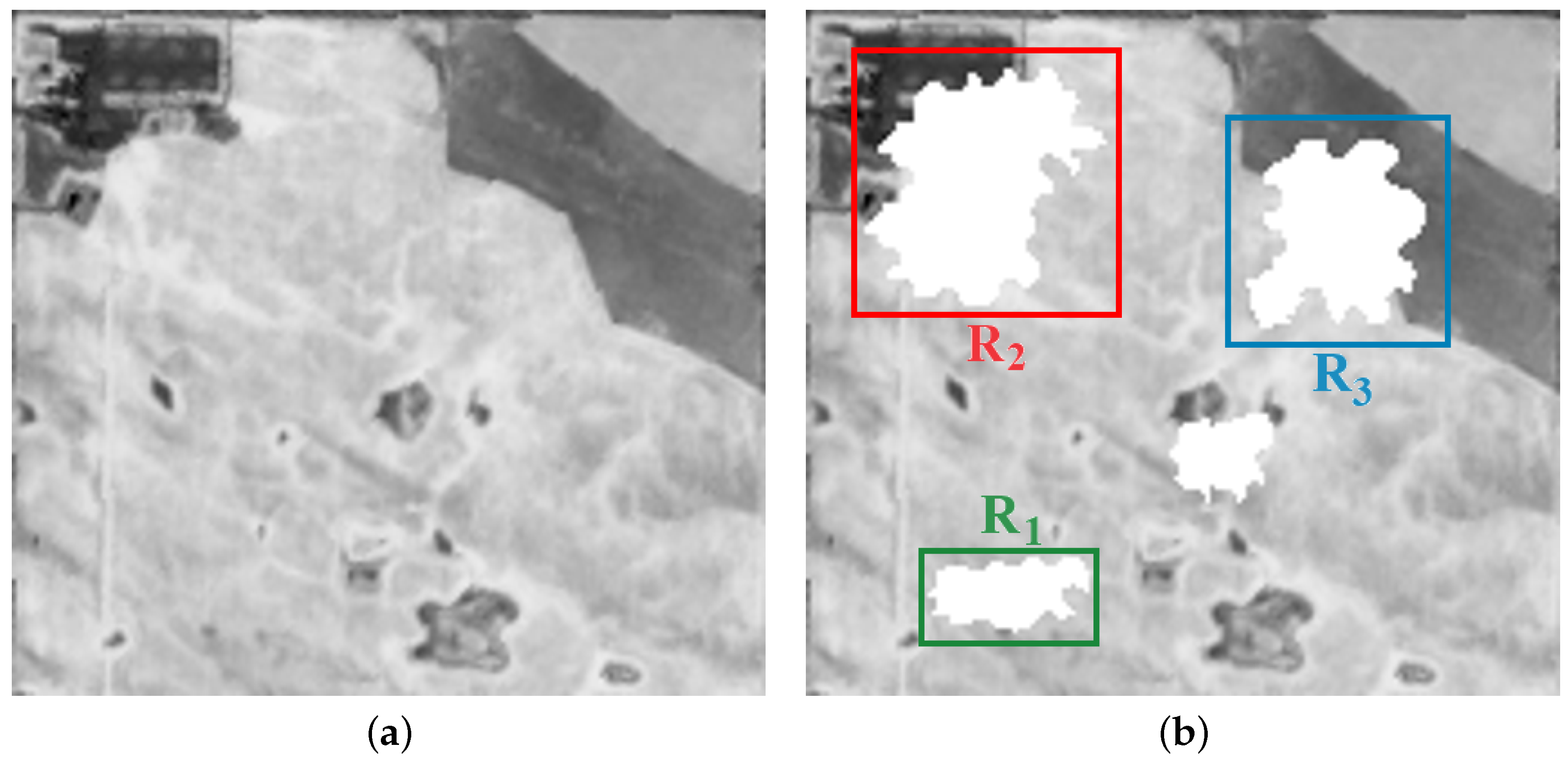
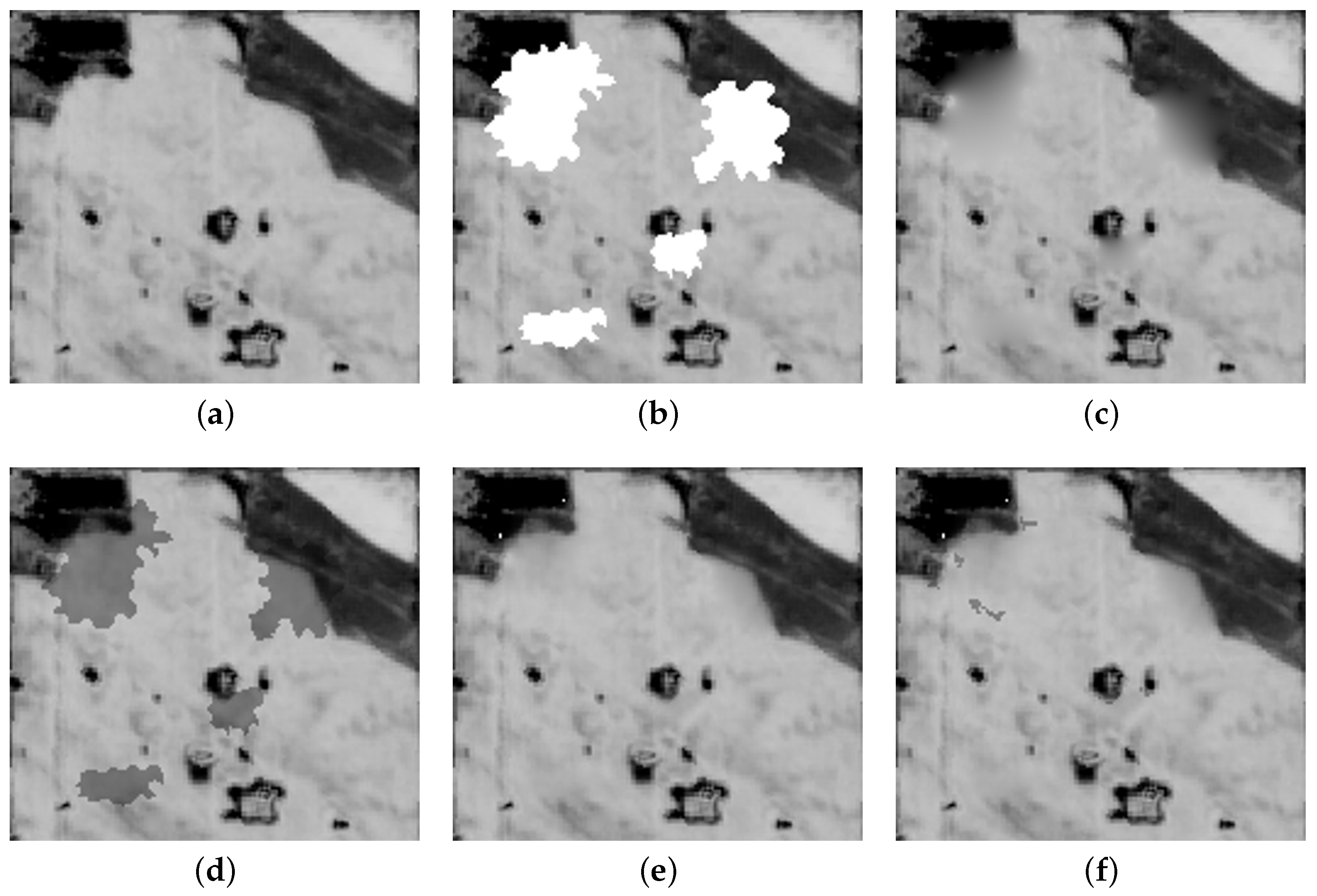
This evaluation was conducted using an assorted set of Sentinel-2 images of a farm field in Alberta, Canada, during the year 2018 with high-resolution images (10 m). There are 52 images from 2018-01-04 to 2018-12-21. For the first case study, we used the NDVI image of the farm related to the date 2018-07-21 (Figure 13a). There are some missing parts containing homogeneous crops (), cropland, buildings (), and a part of a river () (see Figure 13b).

Figure 13.
The original image and the selected regions for Case Study 4.1. (a) Original image. (b) Masked image.
- Experiment 4.1.1.
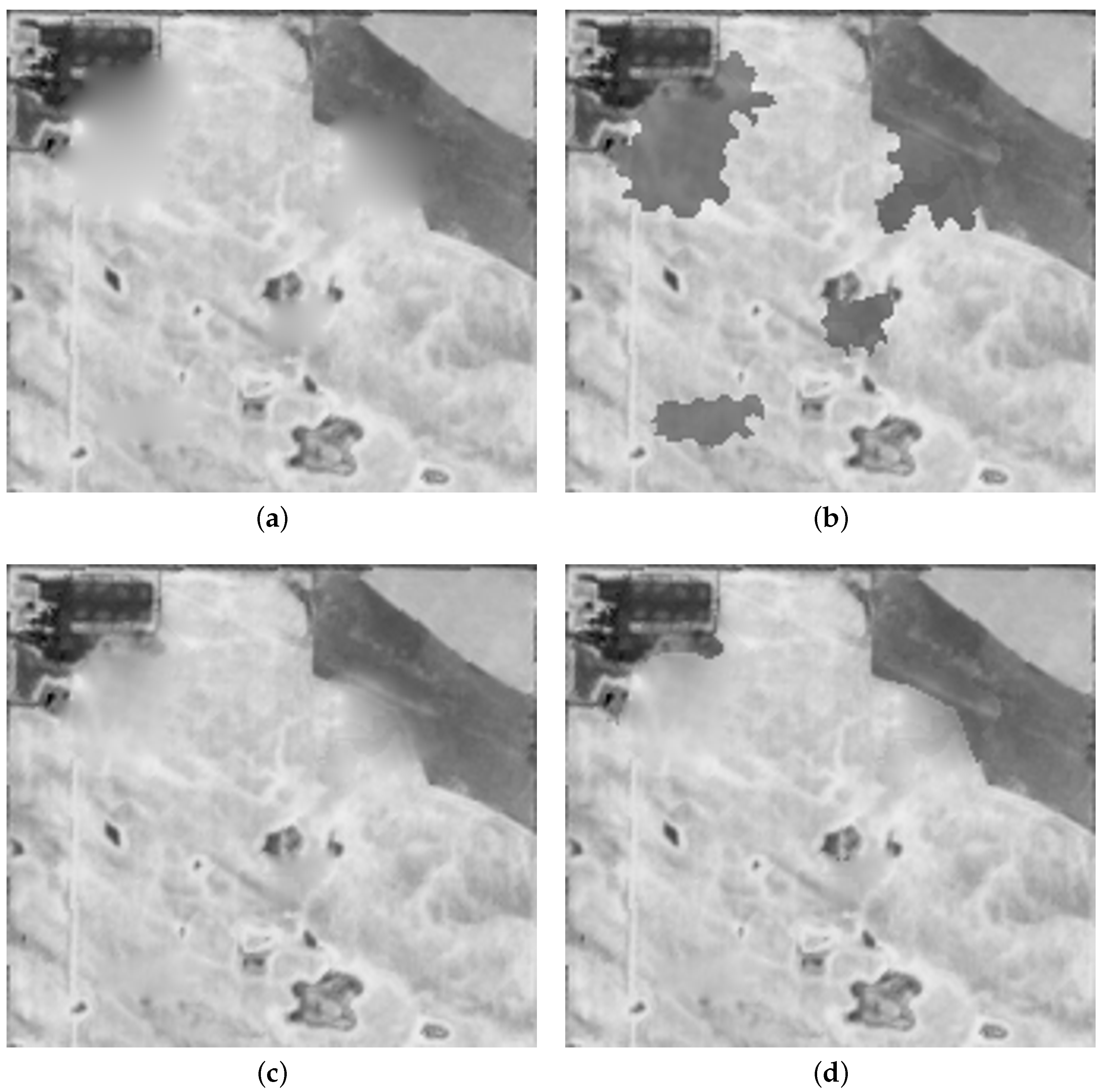
We considered the whole set of NDVI images of the farm to approximate the temporal image and applied a temporal approximation of the four closest dates to the given image. These dates are 2018-07-13, 2018-07-16, 2018-07-18, and 2018-07-26. Table 1 shows the results, and the approximated images are shown in Figure 14.

Table 1.
The evaluated metrics for Experiment 4.1.1.
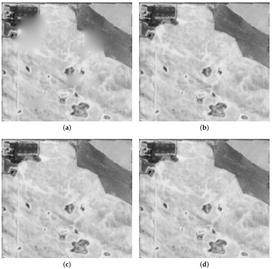
Figure 14.
Approximated NDVI images for Experiment 4.1.1. (a) Spatial approximation. (b) Temporal approximation. (c) Spatial–temporal approximation. (d) Variational spatial–temporal approximation.
The analysis highlights that STPA and BVSTA are the most efficient methods, with STPA being marginally better. Since the used dates are close enough to the desired date, TA has an acceptable performance.
- Experiment 4.1.2.
In this experiment, to approximate the temporal image, we considered the whole set of NDVI images of the farm, but we applied a temporal approximation of the 15 closest dates to the given image. Table 2 shows the results, and the approximated images are shown in Figure 15.

Table 2.
The evaluated metrics for Experiment 4.1.2.

Figure 15.
Approximated NDVI images for Experiment 4.1.2. (a) Spatial approximation. (b) Temporal approximation. (c) Spatial–temporal approximation. (d) Variational spatial–temporal approximation.
The analysis of the whole image shows that BVSTA is the most efficient method; however, STPA has an acceptable performance. The temporal approximation is less efficient since images from distant dates are included.
We tested all approximation methods over the selected local regions , , and . Table 3 shows the results for these regions.

Table 3.
The evaluated metrics for Experiment 4.1.2. over different regions.
The observation of different regions shows that since the variations for region are almost the same in the whole region, there is no difference between STPA and BVSTA. Also, since the region has an almost-homogeneous structure with low variance, the spatial approximation has an acceptable efficiency; however, the spatial–temporal approximations are better than others, and the SA has an acceptable performance. In regions and , STPA and BVSTA are both significantly more efficient than the spatial and temporal approximations.
- Case Study 4.2.
We tested our method on the water index NDWI images with the same farm field (Case Study 4.1). To approximate the temporal image, we applied a weighted least-squares temporal approximation of the 15 closest data points to the given image. Table 4 shows the results for NDWI images and the approximated images in Figure 16.

Table 4.
The evaluated metrics for Case Study 4.2.
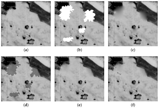
Figure 16.
Approximated NDWI images. (a) Original image. (b) Masked image. (c) Spatial approximation. (d) Temporal approximation. (e) Spatial–temporal approximation. (f) Variational spatial–temporal approximation.
The analysis shows that BVSTA is the most efficient method; however, STPA has an acceptable performance.
- Case Study 4.3.
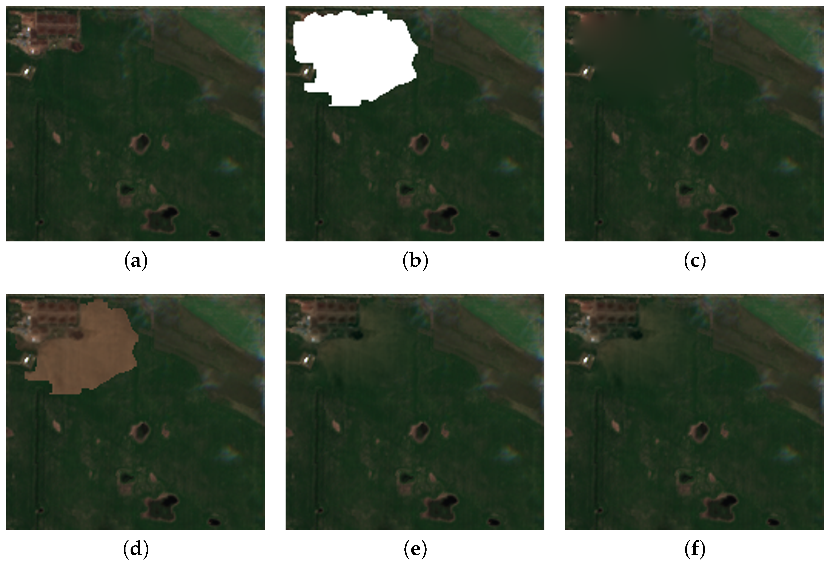
We applied our method to multichannel RGB images. We considered the image taken on 2018-07-08. Also, we applied a temporal approximation of the six closest dates to the given image to approximate the temporal image. Table 5 shows the results for RGB images and the approximated images in Figure 17. In the masked Figure 17b, the missing part contains homogeneous crops, cropland, and buildings.

Table 5.
The evaluated metrics for Case Study 4.3.
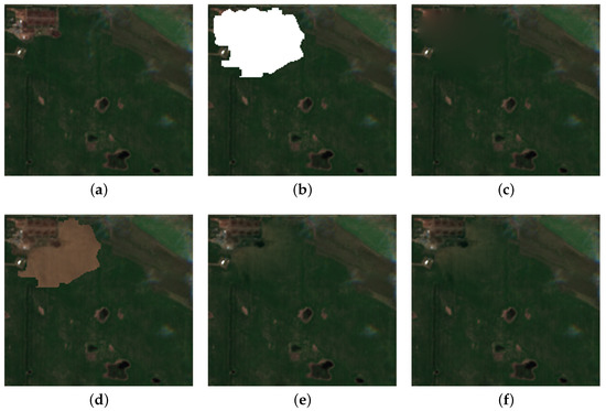
Figure 17.
Approximated RGB images. (a) Original image. (b) Masked image. (c) Spatial approximation. (d) Temporal approximation. (e) Spatial–temporal approximation. (f) Variational spatial–temporal approximation.
The analysis indicates that BVSTA is the most efficient method, while STPA still performs well.
- Case Study 4.4.
For the final case study, we evaluated a diverse collection of high-resolution RGB images captured by a Planet satellite throughout 2022. The images were taken over a farm field located in Alberta, Canada, and had a resolution of 3 m.
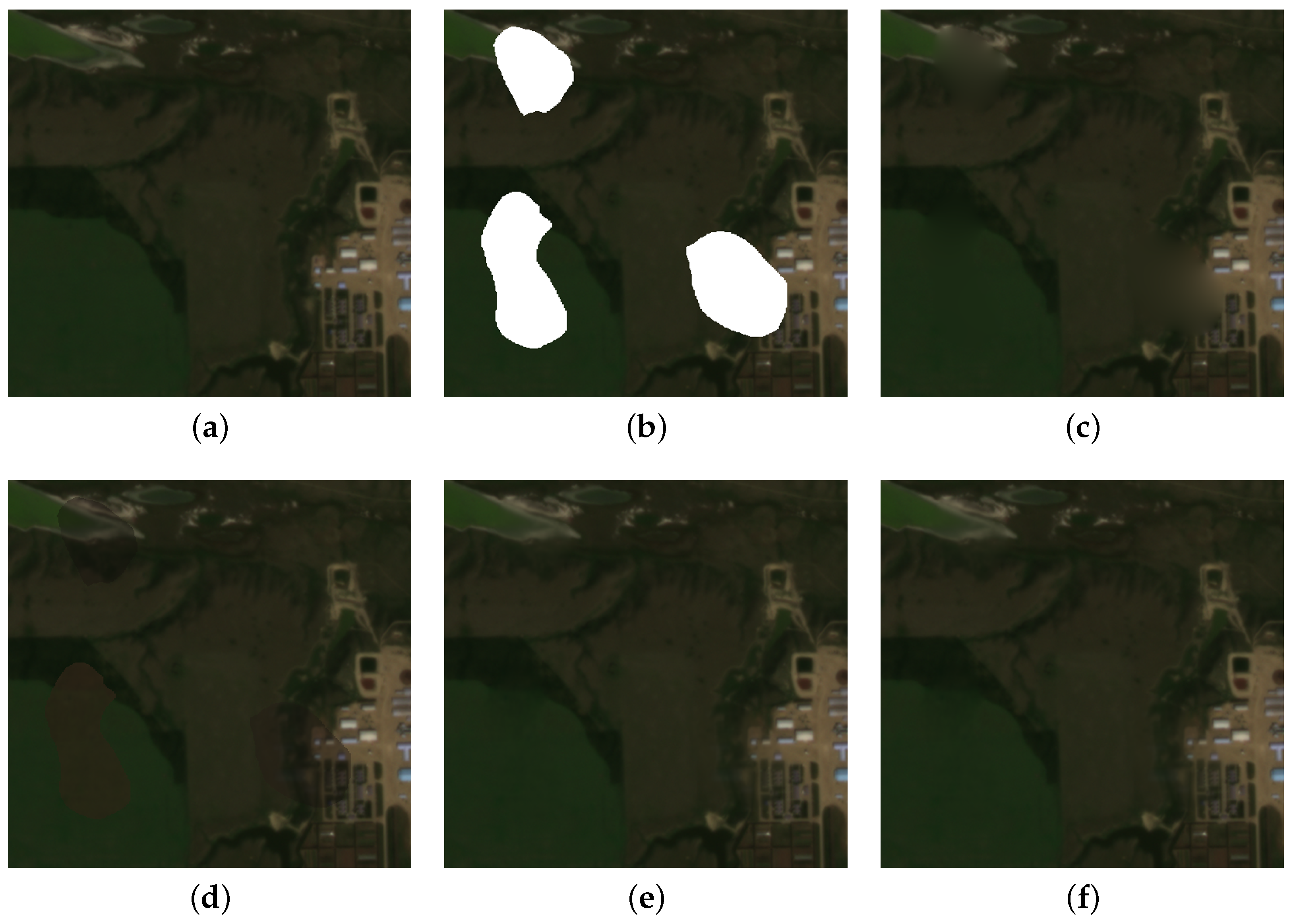
We considered the image taken on 2022-08-19. Also, we applied a temporal approximation of the 10 closest dates to the given image to approximate the temporal image. Table 6 shows the results for RGB images and the approximated images in Figure 18. The missing part in the masked Figure 18b contains homogeneous crops, cropland, and buildings.

Table 6.
The evaluated metrics for Case Study 4.4.

Figure 18.
Approximated RGB images from a Planet satellite. (a) Original image. (b) Masked image. (c) Spatial approximation. (d) Temporal approximation. (e) Spatial–temporal approximation. (f) Variational spatial–temporal approximation.
The analysis indicates that STPA and BVSTA are the most efficient methods, with STPA being slightly superior.
- Case Study 4.5.
This evaluation was conducted using an assorted set of high-resolution (10 m) Sentinel-2 images of a region in Alberta, Canada, captured during the year 2019.
- Experiment 4.5.1.
The image from 2019-07-23 is the target image. We considered the whole set of RGB images of the given region to approximate the temporal image and applied a temporal approximation of the eight closest dates to the given image. Table 7 shows the results, and the approximated images are shown in Figure 19.

Table 7.
The evaluated metrics for Experiment 4.5.1.
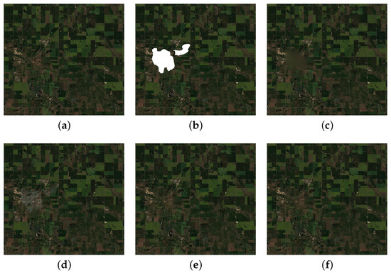
Figure 19.
Approximated RGB images captured by a Planet satellite. (a) Original image. (b) Masked image. (c) Spatial approximation. (d) Temporal approximation. (e) Spatial–temporal approximation. (f) Variational spatial–temporal approximation.
The analysis shows that STPA and BVSTA are the most efficient methods, with STPA being slightly superior. The reconstruction accuracy of both of our methods shows better performance in comparison with the proposed methods in [20] (their provided results have approximately and for croplands) and in [37] (their provided results have approximately and ).
- Experiment 4.5.2.
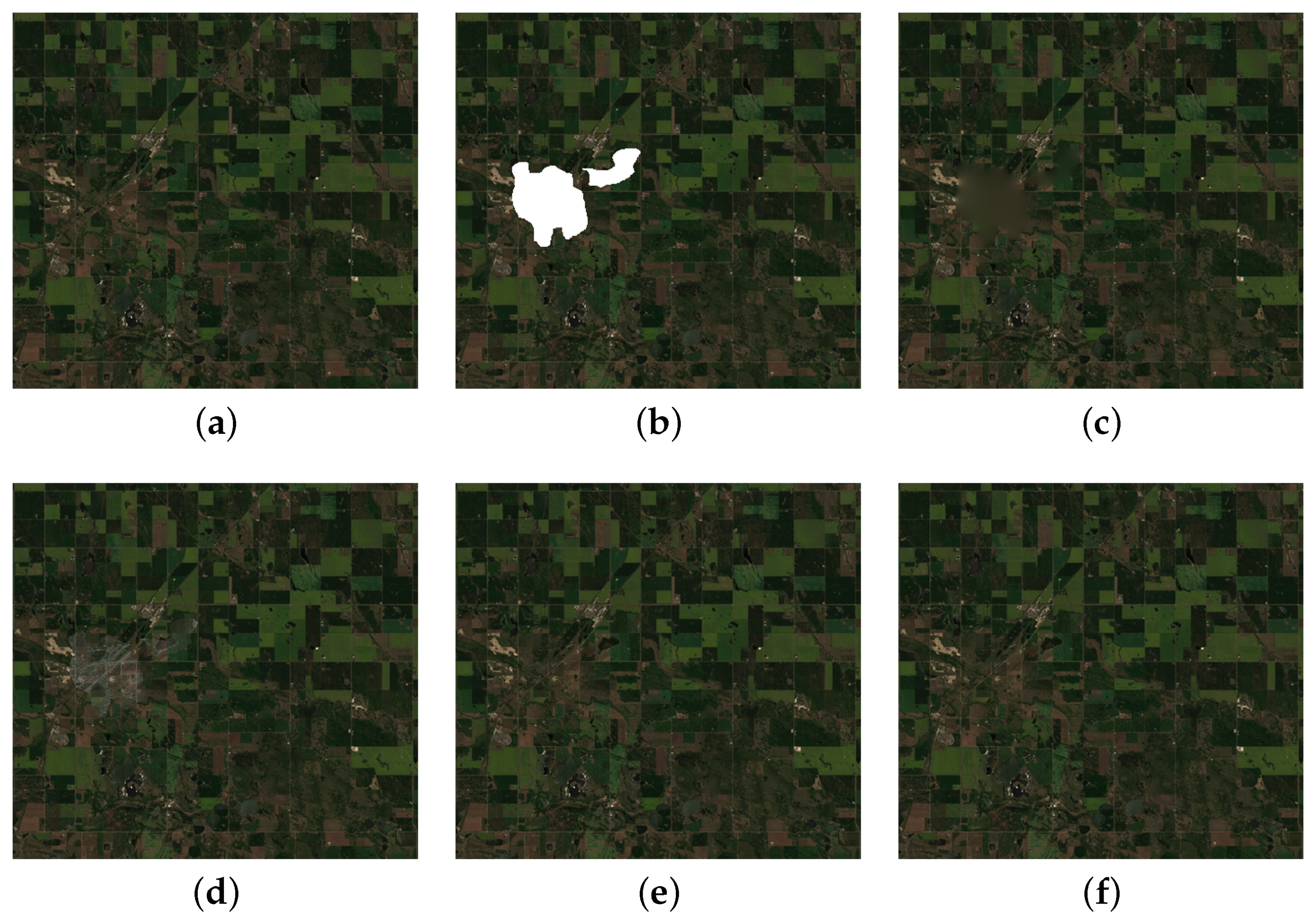
In the original image from 2019-08-02, a large area is covered by clouds and their shadows. We used a set of RGB images of this area to create an approximation of the temporal image and applied this approximation to the 20 closest dates to the given image. The images used for the approximation are displayed in Figure 20.
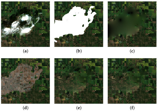
Figure 20.
Approximated RGB images captured by a Planet satellite. (a) Original image. (b) Masked image. (c) Spatial approximation. (d) Temporal approximation. (e) Spatial–temporal approximation. (f) Variational spatial–temporal approximation.
5. Conclusions and Future Directions
In this paper, we present a novel variational model for the spatial–temporal approximation of time-varying satellite imagery, which effectively addresses the issue of missing or masked data caused by clouds and shadows. We developed two innovative methods based on this model, each designed to cater to different scenarios.
The first method extends the Poisson inpainting technique by using a temporal approximation as a guiding vector field, which is achieved through a pixel-wise time-series approximation technique utilizing the weighted least-squares approximation of preceding and subsequent images.
The second method leverages the rate of change in the temporal approximation to divide the missing region into low-variation and high-variation sub-regions. This approach guides the Poisson blending technique for non-homogeneous regions with different variations. By adjusting the relative weights of spatial and temporal components based on the temporal variation at each point, our second method is particularly suitable for specific scenarios in which substantial amounts of temporal data near the target date for reconstruction are missing.
Through rigorous testing, including five different case studies, we demonstrated that our proposed methods outperform conventional temporal and spatial approximation techniques in terms of accuracy and versatility. Our methods resulted in an average increase in accuracy of 190% and 130% compared to spatial and temporal approximations in all case studies.
One drawback of our second method (BVSTA) is the algorithm’s speed. Although its complexity is linear, its constant factor is greater than that of the Poisson inpainting method.
In the future, it will be important to assess the robustness of the parameters in the general variational model by conducting a comprehensive analysis with a wider range of case studies. This may involve determining the threshold parameter when employing the second method. Additionally, there is potential for further exploration by expanding the binarized method into a more flexible and progressive model that operates with multiple sub-regions, rather than just two sub-regions (binary).
Author Contributions
Conceptualization, M.A. and F.F.S.; Methodology, M.A. and F.F.S.; Software, M.A.; Validation, M.A. and F.F.S.; Formal analysis, M.A. and F.F.S.; Writing—original draft, M.A.; Writing—review & editing, M.A. and F.F.S.; Visualization, M.A.; Supervision, F.F.S. All authors have read and agreed to the published version of the manuscript.
Funding
We wish to acknowledge the support of the Mathematics of Information Technology and Complex Systems (MITACS) and the Natural Sciences and Engineering Research Council of Canada (NSERC).
Data Availability Statement
GIS data were obtained from Sentinel Hub services, specifically the Process API: https://docs.sentinel-hub.com/api/latest/api/process/, accessed on 10 March 2023. Planet data were obtained from Planet Labs PBC, Planet Application Program Interface: In Space for Life on Earth: https://api.planet.com, accessed on 12 February 2024.
Acknowledgments
The authors are grateful to the anonymous referees for their valuable comments and suggestions, which have significantly contributed to improving the quality of this paper. We would also like to express our appreciation to Lakin Wecker for the great discussions and insights during the research project and to Christopher Mossman for diligently reviewing the English grammar of this paper. While the funding for this project did not originate from TELUS Agriculture, our collaboration with the company, specifically with Vincent Yeow Chieh Pang, greatly shaped this paper’s research.
Conflicts of Interest
The authors declare no conflicts of interest.
Abbreviations
The following abbreviations are used in this manuscript:
| NDVI | Normalized Difference Vegetation Index |
| NDWI | Normalized Difference Water Index |
| SA | Spatial approximation |
| TA | Temporal approximation |
| STPA | Spatial–temporal approximation |
| BVSTA | Binarized-Variation-Based Spatial–Temporal Approximation |
| RMSE | Root Mean Squared Error |
| PSNR | Peak Signal-to-Noise Ratio |
| MSE | Mean Squared Error |
| SSIM | Structural Similarity Index Metric |
References
- Lambin, E.F.; Linderman, M. Time series of remote sensing data for land change science. IEEE Trans. Geosci. Remote Sens. 2006, 44, 1926–1928. [Google Scholar] [CrossRef]
- Simoes, R.; Camara, G.; Queiroz, G.; Souza, F.; Andrade, P.R.; Santos, L.; Carvalho, A.; Ferreira, K. Satellite Image Time Series Analysis for Big Earth Observation Data. Remote Sens. 2021, 13, 2428. [Google Scholar] [CrossRef]
- Pérez, P.; Gangnet, M.; Blake, A. Poisson image editing. Acm Trans. Graph. 2003, 22, 313–318. [Google Scholar] [CrossRef]
- Di Martino, J.M.; Facciolo, G.; Meinhardt-Llopis, E. Poisson Image Editing. Image Process. Line 2016, 6, 300–325. [Google Scholar] [CrossRef]
- Pérez, P.; Gangnet, M.; Blake, A. Poisson Image Editing. In Seminal Graphics Papers: Pushing the Boundaries, Volume 2, 1st ed.; Association for Computing Machinery: New York, NY, USA, 2023. [Google Scholar]
- Meng, J.; Du, X.; Wu, B. Generation of high spatial and temporal resolution NDVI and its application in crop biomass 732 estimation. Int. J. Digit. Earth 2013, 6, 203–218. [Google Scholar] [CrossRef]
- Atzberger, C.; Formaggio, A.; Shimabukuro, Y.; Udelhoven, T.; Mattiuzzi, M.; Sanchez, G.; Arai, E. Obtaining crop-specific time 735 profiles of NDVI: The use of unmixing approaches for serving the continuity between SPOT-VGT and PROBA-V time series. Int. J. Remote Sens. 2014, 35, 2615–2638. [Google Scholar] [CrossRef]
- Yang, L.; Shen, F.; Zhang, L.; Cai, Y.; Yi, F.; Zhou, C. Quantifying influences of natural and anthropogenic factors on vegetation changes using structural equation modeling: A case study in Jiangsu Province, China. J. Clean. Prod. 2021, 280, 124330. [Google Scholar] [CrossRef]
- Jiang, F.; Deng, M.; Long, Y.; Sun, H. Spatial Pattern and Dynamic Change of Vegetation Greenness From 2001 to 2020 in Tibet, China. Front. Plant Sci. 2022, 13, 892625. [Google Scholar] [CrossRef] [PubMed]
- Ali, A.; de Bie, C.A.J.M.; Skidmore, A.K.; Scarrott, R.G.; Hamad, A.; Venus, V.; Lymberakis, P. Mapping land cover gradients through analysis of hyper-temporal NDVI imagery. Int. J. Appl. Earth Obs. Geoinf. 2013, 23, 301–312. [Google Scholar] [CrossRef]
- Faizal, A.; Mutmainna, N.; Amran, M.A.; Saru, A.; Amri, K.; Nessa, M.N. Application of NDVI Transformation on Sentinel 2A Imagery for mapping mangrove conditions in Makassar City. Akuatikisle Akuakultur Pesisir-Dan-Pulau-Pulau Kecil 2023, 7, 59–66. [Google Scholar] [CrossRef]
- Cheng, Q.; Shen, H.; Zhang, L.; Li, P. Inpainting for Remotely Sensed Images With a Multichannel Nonlocal Total Variation Model. IEEE Trans. Geosci. Remote Sens. 2014, 52, 175–187. [Google Scholar] [CrossRef]
- Shen, H.; Zhang, L. A MAP-Based Algorithm for Destriping and Inpainting of Remotely Sensed Images. IEEE Trans. Geosci. Remote Sens. 2009, 47, 1492–1502. [Google Scholar] [CrossRef]
- Hu, Y.; Wei, Z.; Zhao, K. Remote Sensing Images Inpainting based on Structured Low-Rank Matrix Approximation. In Proceedings of the IGARSS 2020–2020 IEEE International Geoscience and Remote Sensing Symposium, Waikoloa, HI, USA, 26 September–2 October 2020; pp. 1341–1344, ISSN 2153-7003. [Google Scholar] [CrossRef]
- Amrani, N.; Serra-Sagristà, J.; Peter, P.; Weickert, J. Diffusion-Based Inpainting for Coding Remote-Sensing Data. IEEE Geosci. Remote Sens. Lett. 2017, 14, 1203–1207. [Google Scholar] [CrossRef]
- Farbman, Z.; Fattal, R.; Lischinski, D.; Szeliski, R. Edge-preserving decompositions for multi-scale tone and detail manipulation. Acm Trans. Graph. 2008, 27, 1–10. [Google Scholar] [CrossRef]
- Sun, J.; Jia, J.; Tang, C.K.; Shum, H.Y. Poisson matting. In ACM SIGGRAPH 2004 Papers; ACM Digital Library: New York, NY, USA, 2004; Volume 23, pp. 315–321. [Google Scholar] [CrossRef]
- Wu, H.; Zheng, S.; Zhang, J.; Huang, K. GP-GAN: Towards Realistic High-Resolution Image Blending. In Proceedings of the 27th ACM International Conference on Multimedia, Nice, France, 21–25 October 2019; Association for Computing Machinery: New York, NY, USA, 2019. MM’19. pp. 2487–2495. [Google Scholar] [CrossRef]
- Tanaka, M.; Kamio, R.; Okutomi, M. Seamless image cloning by a closed form solution of a modified Poisson problem. In Proceedings of the SIGGRAPH Asia 2012 Posters, Singapore, 28 November–1 December 2012; ACM: New York, NY, USA, 2012; p. 1. [Google Scholar] [CrossRef]
- Hu, C.; Huo, L.Z.; Zhang, Z.; Tang, P. Multi-Temporal Landsat Data Automatic Cloud Removal Using Poisson Blending. IEEE Access 2020, 8, 46151–46161. [Google Scholar] [CrossRef]
- Lan, S.; Dong, Z. Incorporating Vegetation Type Transformation with NDVI Time-Series to Study the Vegetation Dynamics in Xinjiang. Sustainability 2022, 14, 582. [Google Scholar] [CrossRef]
- Zhou, Y.N.; Wang, S.; Wu, T.; Feng, L.; Wu, W.; Luo, J.; Zhang, X.; Yan, N.N. For-backward LSTM-based missing data reconstruction for time-series Landsat images. GIScience Remote Sens. 2022, 59, 410–430. [Google Scholar] [CrossRef]
- Inglada, J.; Vincent, A.; Arias, M.; Tardy, B.; Morin, D.; Rodes, I. Operational High Resolution Land Cover Map Production at the Country Scale Using Satellite Image Time Series. Remote Sens. 2017, 9, 95. [Google Scholar] [CrossRef]
- Liu, M.; Yang, W.; Zhu, X.; Chen, J.; Chen, X.; Yang, L.; Helmer, E.H. An Improved Flexible Spatiotemporal DAta Fusion (IFSDAF) method for producing high spatiotemporal resolution normalized difference vegetation index time series. Remote Sens. Environ. 2019, 2019. 227, 74–89. [Google Scholar] [CrossRef]
- Zhou, J.; Sun, W.; Meng, X.; Yang, G.; Ren, K.; Peng, J. Generalized Linear Spectral Mixing Model for Spatial–Temporal–Spectral Fusion. IEEE Trans. Geosci. Remote Sens. 2022, 60, 5533216. [Google Scholar] [CrossRef]
- He, S.; Shao, H.; Xian, W.; Zhang, S.; Zhong, J.; Qi, J. Extraction of Abandoned Land in Hilly Areas Based on the Spatio-Temporal Fusion of Multi-Source Remote Sensing Images. Multidiscip. Digit. Publ. Inst. 2021, 13, 3956. [Google Scholar] [CrossRef]
- Rao, Y.; Zhu, X.; Chen, J.; Wang, J. An Improved Method for Producing High Spatial-Resolution NDVI Time Series Datasets with Multi-Temporal MODIS NDVI Data and Landsat TM/ETM+ Images. Multidiscip. Digit. Publ. Inst. 2015, 7, 7865–7891. [Google Scholar] [CrossRef]
- Xue, L.; Sheng, Y.; Liu, Y.; Zhang, K. A reliable matching algorithm for heterogeneous remote sensing images considering the spatial distribution of matched features. Int. J. Remote Sens. 2023, 44, 824–851. [Google Scholar] [CrossRef]
- Shen, Z.; Wang, Y.; Su, H.; He, Y.; Li, S. A bi-directional strategy to detect land use function change using time-series Landsat imagery on Google Earth Engine: A case study of Huangshui River Basin in China. Sci. Remote Sens. 2022, 5, 100039. [Google Scholar] [CrossRef]
- Chen, H.; Shi, Z. A Spatial-Temporal Attention-Based Method and a New Dataset for Remote Sensing Image Change Detection. Multidiscip. Digit. Publ. Inst. 2020, 12, 1662. [Google Scholar] [CrossRef]
- Chen, Y.; Ge, Y. Spatiotemporal image fusion using multiscale attention-aware two-stream convolutional neural networks. Sci. Remote Sens. 2022, 6, 100062. [Google Scholar] [CrossRef]
- Shao, Z.; Wu, W.; Li, D. Spatio-temporal-spectral observation model for urban remote sensing. Geo-Spat. Inf. Sci. 2021, 24, 372–386. [Google Scholar] [CrossRef]
- Zhu, F.; Wang, C.; Zhu, B.; Sun, C.; Qi, C. An improved generative adversarial networks for remote sensing image super-resolution reconstruction via multi-scale residual block. Egypt. J. Remote Sens. Space Sci. 2023, 26, 151–160. [Google Scholar] [CrossRef]
- Jiang, B.; Li, X.; Chong, H.; Wu, Y.; Li, Y.; Jia, J.; Wang, S.; Wang, J.; Chen, X. A deep-learning reconstruction method for remote sensing images with large thick cloud cover. Int. J. Appl. Earth Obs. Geoinf. 2022, 115, 103079. [Google Scholar] [CrossRef]
- Chen, H.; Qi, Z.; Shi, Z. Remote Sensing Image Change Detection with Transformers. IEEE Trans. Geosci. Remote Sens. 2022, 60, 1–14. [Google Scholar] [CrossRef]
- Chen, Y.; Weng, Q.; Tang, L.; Zhang, X.; Bilal, M.; Li, Q. Thick Clouds Removing From Multitemporal Landsat Images Using Spatiotemporal Neural Networks. IEEE Trans. Geosci. Remote Sens. 2022, 60, 4400214. [Google Scholar] [CrossRef]
- Long, C.; Li, X.; Jing, Y.; Shen, H. Bishift Networks for Thick Cloud Removal with Multitemporal Remote Sensing Images. Int. J. Intell. Syst. 2023, 2023, 46151–46161. [Google Scholar] [CrossRef]
- Duan, C.; Pan, J.; Li, R. Thick Cloud Removal of Remote Sensing Images Using Temporal Smoothness and Sparsity Regularized Tensor Optimization. Multidiscip. Digit. Publ. Inst. 2020, 12, 3446. [Google Scholar] [CrossRef]
- Valero, S.; Morin, D.; Inglada, J.; Sepulcre, G.; Arias, M.; Hagolle, O.; Dedieu, G.; Bontemps, S.; Defourny, P.; Koetz, B. Production of a Dynamic Cropland Mask by Processing Remote Sensing Image Series at High Temporal and Spatial Resolutions. Multidiscip. Digit. Publ. Inst. 2016, 8, 55. [Google Scholar] [CrossRef]
- Wang, Y.; Zhang, W.; Chen, S.; Li, Z.; Zhang, B. Rapidly Single-Temporal Remote Sensing Image Cloud Removal based on Land Cover Data. In Proceedings of the IGARSS 2022—2022 IEEE International Geoscience and Remote Sensing Symposium, Kuala Lumpur, Malaysia, 17–22 July 2022; pp. 3307–3310, ISSN 2153-7003. [Google Scholar] [CrossRef]
- Ebel, P.; Xu, Y.; Schmitt, M.; Zhu, X. SEN12MS-CR-TS: A Remote Sensing Data Set for Multi-modal Multi-temporal Cloud Removal. IEEE Trans. Geosci. Remote Sens. 2022, 60, 1–14. [Google Scholar] [CrossRef]
- Layton, J.C.; Wecker, L.; Runions, A.; Samavati, F.F. Cloud Shadow Detection via Ray Casting with Probability Analysis Refinement Using Sentinel-2 Satellite Data. Multidiscip. Digit. Publ. Inst. 2023, 15, 3955. [Google Scholar] [CrossRef]
- Talordphop, K.; Sukparungsee, S.; Areepong, Y. On designing new mixed modified exponentially weighted moving average—Exponentially weighted moving average control chart. Results Eng. 2023, 18, 101152. [Google Scholar] [CrossRef]
- Wang, J.; Pei, Z.K.; Wang, Y.; Qin, Z. An investigation of income inequality through autoregressive integrated moving average and regression analysis. Healthc. Anal. 2024, 5, 100287. [Google Scholar] [CrossRef]
- Xing, Y.; Song, Q.; Cheng, G. Benefit of Interpolation in Nearest Neighbor Algorithms. SIAM J. Math. Data Sci. 2022, 4, 935–956. [Google Scholar] [CrossRef]
- Samworth, R.J. Optimal weighted nearest neighbour classifiers. Inst. Math. Stat. 2012, 40, 2733–2763. [Google Scholar] [CrossRef]
- Amirfakhrian, M.; Samavati, F. Weather daily data approximation using point adaptive ellipsoidal neighborhood in scattered data interpolation methods. Appl. Math. Comput. 2021, 392, 125717. [Google Scholar] [CrossRef]
- Bartels, R.H.; Golub, G.H.; Samavati, F.F. Some observations on local least squares. BIT Numer. Math. 2006, 46, 455–477. [Google Scholar] [CrossRef]
- Bemporad, A. Active learning for regression by inverse distance weighting. Bit Numer. Math. 2023, 626, 275–292. [Google Scholar] [CrossRef]
- Li, F.; Shang, Z.; Liu, Y.; Shen, H.; Jin, Y. Inverse distance weighting and radial basis function based surrogate model for high-dimensional expensive multi-objective optimization. Appl. Soft Comput. 2024, 152, 111194. [Google Scholar] [CrossRef]
- Soudani, K.; le Maire, G.; Dufrêne, E.; François, C.; Delpierre, N.; Ulrich, E.; Cecchini, S. Evaluation of the onset of green-up in temperate deciduous broadleaf forests derived from Moderate Resolution Imaging Spectroradiometer (MODIS) data. Remote Sens. Environ. 2008, 112, 2643–2655. [Google Scholar] [CrossRef]
- Özüm Durgun, Y.; Gobin, A.; Duveiller, G.; Tychon, B. A study on trade-offs between spatial resolution and temporal sampling density for wheat yield estimation using both thermal and calendar time. Int. J. Appl. Earth Obs. Geoinf. 2020, 86, 101988. [Google Scholar] [CrossRef]
- Zhong, L.; Gong, P.; Biging, G.S. Efficient corn and soybean mapping with temporal extendability: A multi-year experiment using Landsat imagery. Remote Sens. Environ. 2014, 140, 1–13. [Google Scholar] [CrossRef]
- Vorobiova, N.; Chernov, A. Curve fitting of MODIS NDVI time series in the task of early crops identification by satellite images. Procedia Eng. 2017, 201, 184–195. [Google Scholar] [CrossRef]
- Tan, L.; Liu, W.; Pan, Z. Color image restoration and inpainting via multi-channel total curvature. Appl. Math. Model. 2018, 61, 280–299. [Google Scholar] [CrossRef]
- Hoeltgen, L.; Kleefeld, A.; Harris, I.; Breuss, M. Theoretical foundation of the weighted laplace inpainting problem. Appl. Math. 2019, 64, 281–300. [Google Scholar] [CrossRef]
- Gockenbach, M.S. Understanding and Implementing the Finite Element Method; Other Titles in Applied Mathematics, Society for Industrial and Applied Mathematics: Philadelphia, PA, USA, 2006. [Google Scholar] [CrossRef]
- Strauss, W.A. Partial Differential Equations: An Introduction, 2nd ed.; John Wiley: Hoboken, NJ, USA, 2018. [Google Scholar]
- Al-Khaled, K. Numerical solutions of the Laplace’s equation. Appl. Math. Comput. 2005, 170, 1271–1283. [Google Scholar] [CrossRef]
- Shojaei, I.; Rahami, H.; Kaveh, A. A numerical solution for Laplace and Poisson’s equations using geometrical transformation and graph products. Appl. Math. Model. 2016, 40, 7768–7783. [Google Scholar] [CrossRef]
- Jensen, J.R. Remote Sensing: The Image of Earth; Pearson Prentice Hall: Hoboken, NJ, USA, 2007. [Google Scholar]
- van Belle, G. Statistical Rules of Thumb; Wiley Series in Probability and Statistics; Wiley: Hoboken, NJ, USA, 2011. [Google Scholar]
- Li, H.; Calder, C.A.; Cressie, N. Beyond Moran’s I: Testing for Spatial Dependence Based on the Spatial Autoregressive Model. Geogr. Anal. 2007, 39, 357–375. [Google Scholar] [CrossRef]
- Hyndman, R.J.; Athanasopoulos, G. Forecasting: Principles and Practice, 2nd ed.; OTexts: Melbourne, Australia, 2018; Chapter 3.3; Available online: https://otexts.com/fpp3 (accessed on 12 February 2024).
- Gonzalez, R.C.; Woods, R.E. Digital Image Processing, 4th ed.; Pearson: London, UK, 2018. [Google Scholar]
- Bishop, C.M. Pattern Recognition and Machine Learning; Springer: Berlin/Heidelberg, Germany, 2006. [Google Scholar]
- Wang, Z.; Bovik, A.C.; Sheikh, H.R.; Simoncelli, E.P. Image quality assessment: From error visibility to structural similarity. IEEE Trans. Image Process. 2004, 13, 600–612. [Google Scholar] [CrossRef] [PubMed]
- Lara-Alvarez, C.; Flores, J.J.; Rodriguez-Rangel, H.; Lopez-Farias, R. A literature review on satellite image time series forecasting: Methods and applications for remote sensing. WIREs Data Min. Knowl. Discov. 2024, 14, e1528. [Google Scholar] [CrossRef]
- Zhang, Z.; Tang, P.; Zhang, W.; Tang, L. Satellite Image Time Series Clustering via Time Adaptive Optimal Transport. Remote Sens. 2021, 13, 3993. [Google Scholar] [CrossRef]
Disclaimer/Publisher’s Note: The statements, opinions and data contained in all publications are solely those of the individual author(s) and contributor(s) and not of MDPI and/or the editor(s). MDPI and/or the editor(s) disclaim responsibility for any injury to people or property resulting from any ideas, methods, instructions or products referred to in the content. |
© 2024 by the authors. Licensee MDPI, Basel, Switzerland. This article is an open access article distributed under the terms and conditions of the Creative Commons Attribution (CC BY) license (https://creativecommons.org/licenses/by/4.0/).

