Article

InSAR Analysis of Post-Liquefaction Consolidation Subsidence after 2012 Emilia Earthquake Sequence (Italy)

by
Matteo Albano
1,
Anna Chiaradonna
2,
Michele Saroli
1,3,*,
Marco Moro
1,
Antonio Pepe
4 and
Giuseppe Solaro
4
1
Istituto Nazionale di Geofisica e Vulcanologia, Via di Vigna Murata 605, 00143 Rome, Italy
2
Department of Civil, Construction-Architectural and Environmental Engineering, University of L’Aquila, Piazzale Ernesto Pontieri 1, Monteluco di Roio, 67100 L’Aquila, Italy
3
Dipartimento di Ingegneria Civile e Meccanica, Università degli Studi di Cassino e del Lazio Meridionale, Via G. di Biasio 43, 03043 Cassino, Italy
4
National Research Council of Italy (CNR), Istituto per il Rilevamento Elettromagnetico dell’Ambiente, Via Diocleziano 328, 80124 Naples, Italy
*
Author to whom correspondence should be addressed.
Remote Sens. 2024, 16(13), 2364; https://doi.org/10.3390/rs16132364
Submission received: 13 May 2024 / Revised: 20 June 2024 / Accepted: 24 June 2024 / Published: 28 June 2024

Abstract

:
On 20 May 2012, an Mw 5.8 earthquake, followed by an Mw 5.6 event nine days later, struck the Emilia-Romagna region in northern Italy, causing substantial damage and loss of life. Post-mainshock, several water-related phenomena were observed, such as changes in the groundwater levels in wells, the expulsion of sand–water mixtures, and widespread liquefaction evidence such as sand boils and water leaks from cracks. We analyzed the Earth’s surface displacement during and after the Emilia 2012 seismic sequence using synthetic aperture radar images from the COSMO-SkyMed satellite constellation. This analysis revealed post-seismic ground subsidence between the Sant’Agostino and Mirabello villages. Specifically, the displacement time series showed a slight initial uplift followed by rapid subsidence over approximately four to five months. This widespread ground displacement pattern likely stemmed from the extensive liquefaction of saturated sandy layers at depth. This phenomenon typically induces immediate post-seismic subsidence. However, the observed asymptotic subsidence, reaching about 2.1 cm, suggested a time-dependent process related to post-liquefaction consolidation. To test this hypothesis, we analytically estimated the consolidation subsidence resulting from earthquake-induced excess pore pressure dissipation in the layered soil deposits. The simulated subsidence matched the observed data, further validating the significant role of excess pore pressure dissipation induced by earthquake loading in post-seismic ground subsidence.

1. Introduction

Soil liquefaction represents a prominent phenomenon triggered by seismic motion, particularly relevant in regions where loose, water-saturated sandy layers are confined within impermeable strata close to earthquake epicenters. The ground motion during earthquakes can induce excess pore pressures and temporary losses of strength in these saturated sediments, causing them to behave akin to fluids. Frequently observed in alluvial and coastal plains due to distinct subsurface stratigraphy, liquefaction events have historically caused significant damage to critical infrastructures, agricultural areas, and properties, as exemplified by notable seismic sequences such as the 1810–1811 New Madrid earthquakes [1], the 1964 Alaska and Niigata earthquakes [2,3], the events in Kobe (1995), Chi-Chi (1999), and Izmit (1999) [4,5,6], the Canterbury earthquake of 2010–2011 in New Zealand [7], the Emilia earthquake sequence of 2012 in the Po Plain, Northern Italy [8], and the 2018 Palu earthquake in Indonesia [9].
Liquefaction primarily stems from the generation of excess pore pressures in loose sand deposits subjected to cyclic loading during earthquakes. These deposits may liquefy under seismic stress, resulting in significant losses of stiffness and strength [10]. Structures built atop such deposits face considerable risk of damage from coseismic shear stresses and subsequent post-liquefaction reconsolidation, during which, excess pore pressures gradually dissipate [11,12,13]. In cases where the sand deposit allows drainage only from the base (singly draining), pore fluid flows upward, prolonging the liquefied state of sandy layers at depth and extending the pore pressure dissipation time, thus causing further delayed subsidence. The damage induced by liquefaction arises from intricate interactions among various mechanisms, with post-liquefaction reconsolidation playing a significant role in sand deformation [14,15]. Measuring the extent, amplitude, and temporal evolution of liquefaction-induced ground subsidence is, then, crucial to understanding this phenomenon [12] and contributes to the hazard assessment of liquefaction-prone areas. Unfortunately, such measurements are often difficult to perform because of the spatial and temporal variability of the observed phenomenon.
Nowadays, the Interferometric Synthetic Aperture Radar (InSAR) technique is extensively adopted to map regional- to local-scale surface deformations caused by earthquakes, volcanoes, lava flows, ground subsidence, and landslides [16,17,18,19,20], providing a synoptic and precise measurement of the deformations at the ground with unprecedented spatial coverage over both space and time.
InSAR displacement time series have been successfully applied to monitor pre- and post-earthquake ground movements of tectonic origin [21,22], but there has been limited exploration of using SAR for remotely sensing liquefaction phenomena and mapping local liquefaction-induced effects at the ground, i.e., sand boils and water leaks from cracks. Primarily, complex coherence, which measures how much a scene has changed between two acquisitions, enabled the detection of differential compaction- or liquefaction-induced failure at the scale of building blocks, along with the identification of expelled sands and water. A few case studies have exploited the InSAR technique to detect the local ground subsidence caused by sand ejecta at the surface [13,23,24,25]. However, none of these studies provided insights into the spatial and temporal evolution of post-liquefaction consolidation subsidence, which could last for a long time, depending on the geomorphological setting of the subsoil, further threatening infrastructures at the surface.
This research study utilized high-resolution X-band SAR data collected by COSMO-SkyMed satellites to detect and monitor, for the first time, post-liquefaction ground subsidence during the 2012 Emilia seismic sequence in northern Italy [26]. The study employed a combined SAR-based analysis and geological–geotechnical approach to investigate and quantify the effects of liquefaction, including ground subsidence, and demonstrate their correspondence with InSAR observations.
Analysis of the SAR data unveiled postseismic ground surface subsidence between the villages of Sant’Agostino and Mirabello (nowadays, the Terre del Reno Municipality). The observed displacement time series indicated a minor initial uplift, followed by rapid subsidence that gradually lessened over approximately three to six months. This widespread ground displacement pattern was closely associated with the extensive liquefaction and post-liquefaction consolidation of deep sandy layers, spreading all over the study area.

2. The Case Study

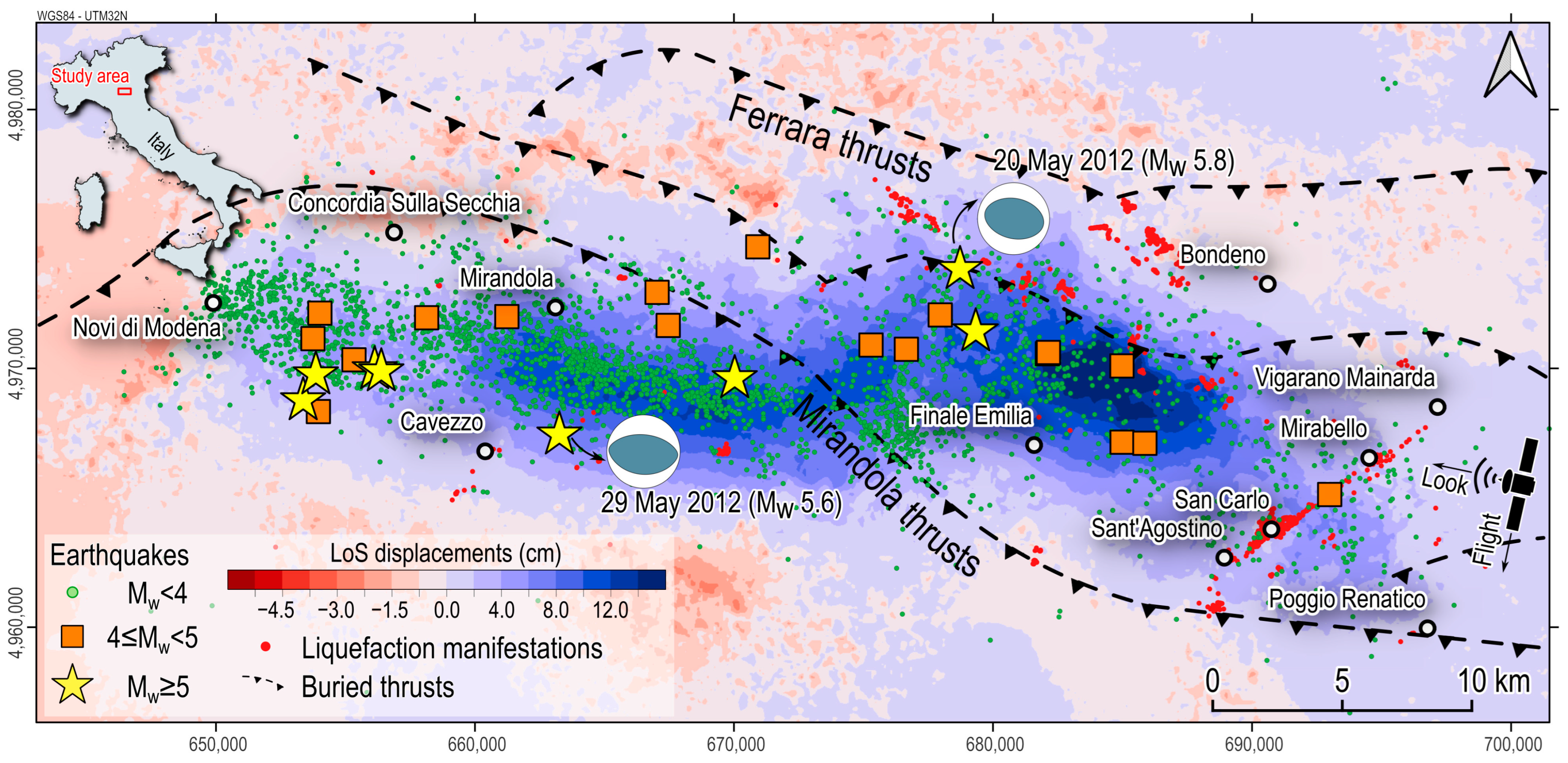
2.1. The Seismic Sequence

On 20 May 2012, the Emilia-Romagna region in northern Italy was struck by an Mw 5.8 earthquake (Figure 1), resulting in devastating damage and loss of life. In the following days, thousands of aftershocks were enucleated, six with a magnitude greater than 5, with the most significant aftershock, measuring Mw 5.6, occurring on 29 May [27] (Figure 1). The seismic activity activated two segments of the Ferrara-Romagna thrust system, namely the Ferrara thrusts and the Mirandola thrusts (Figure 1).
The rupture initially propagated eastward and downdip on the Ferrara thrust system. Then, it moved westward on the adjacent Mirandola thrust, leading to the Mw 5.6 aftershock [26,27]. The moment tensor solutions for the stronger events displayed a reverse focal mechanism [28]. More than 70% of the earthquakes occurred within three months after the first shock, while the events with a magnitude greater than five happened in the first 15 days.
A whole picture of the regional ground displacement pattern is provided first by two Radarsat-2 (RSAT-2) SAR images, acquired on 30 April and 17 June 2012, respectively, and spanning both the 20 and 29 May main events [29,30]. The unwrapped interferogram (Figure 1) shows that the ground moved toward the satellite Line of Sight (LoS) (positive values in (Figure 1) over an area encompassing the seismic activity in the hanging wall of the main shocks. A significant component of this motion involved uplift across the Ferrara and Mirandola thrust faults, peaking at approximately 16 cm close to the Finale Emilia town [26,29].
Figure 1. Sketch of the area affected by the 2012 Emilia earthquake sequence. The thrusts of Ferrara and Mirandola depict the tectonic framework (from Cheloni et al. [26]). The color map shows the unwrapped co-seismic displacements along the Line of Sight of the descending track of the RSAT-2 satellite mission encompassing the 20 and 29 May events (30 April–17 June 2012; side-looking angle 30°; negative and positive values identify movements away and towards the satellite sensor, respectively; modified from Tizzani et al. [29] and Albano et al. [30]). The location of liquefaction phenomena is provided by Emergeo Working Group [31]. The dashed purple line identifies the partial boundary of the COSMO-SkyMed (CSK) SAR frame, located over the Sant’Agostino, San Carlo, and Mirabello villages. Seismicity is available from the INGV database (https://terremoti.ingv.it/, accessed on 8 February 2024).
Remotesensing 16 02364 g001
The study area corresponds to the buried frontal portion of the compressive ramp and flat structures of the Apennines [32]. The earthquake sequence occurred over an alluvial plain representing the surface expression of the foredeep basin of the Apennine chain, where a combination of fast subsidence and substantial sediment input generated very thick Plio-Pleistocene successions made of alternating layers of coarse-grained and fine-grained deposits [33].
In this context, many phenomena occurred after the mainshock. Wells near the epicentral area experienced a sudden increase in water level [34], testifying to a sustained regional perturbation of the deep and shallow aquifers because of tectonic dislocation [30,35,36]. Periodic sampling of the liquid and gaseous phases in surficial aquifers also indicated a rise in deep-seated fluids along faults and fractures, which altered the geochemical composition of fluids belonging to shallower aquifers [37].
Additionally, over 700 liquefaction phenomena were observed, particularly in the area encompassed by the San Carlo and Sant’Agostino villages [31,38] (red dots in Figure 1 and Figure 2a,b). Sand boils, water leaks from cracks at the ground surface, gravitational lateral spreading, and a widespread pattern of ground subsidence were reported, often distributed along elongated strips, corresponding to fluvial buried sandy bodies of the Holocene age [39]. The formation of a coalescent system of flat extensional fractures with small vertical throws along preferential alignments accompanied these phenomena. These fractures caused significant vertical offsets and the outcropping of fine sand from fractures, forming extensive heaps.

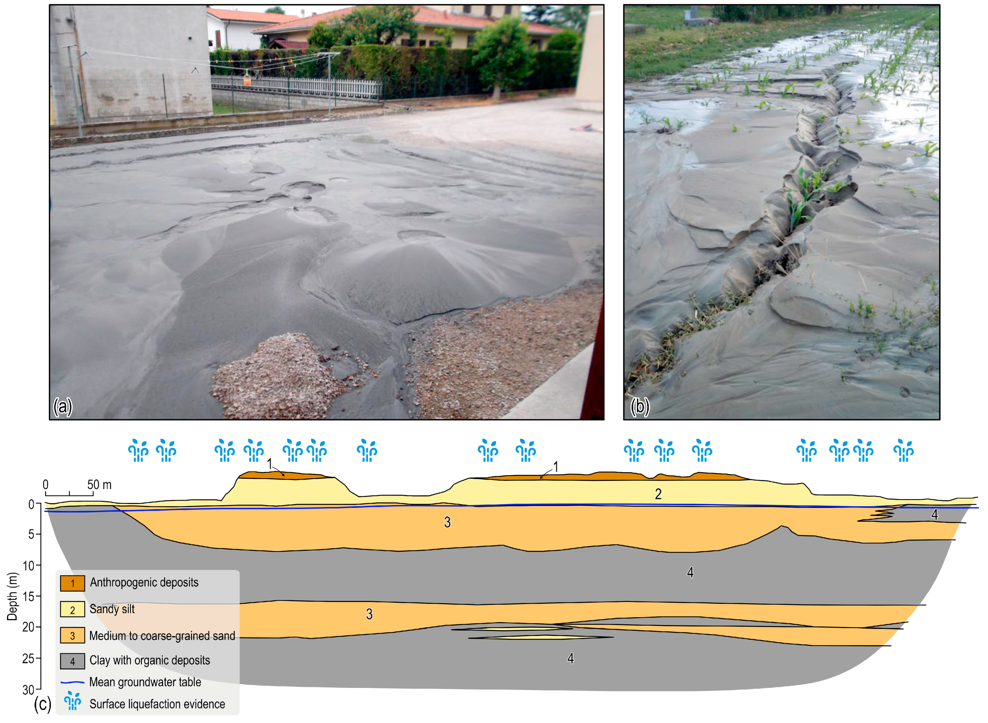
2.2. Lithological Setting of the Area

Several authors have synthesized the subsoil characterizing the Sant’Agostino, San Carlo, and Mirabello areas [8,40,41,42]. The typical stratigraphy, as reported in Figure 2c, consists, from top to bottom, of shallow sandy and clayey silts (about 4 m in thickness each); intermediate sands from an 8 to 2 m depth; intermediate clays (5 to 10 m thick); deep sands (3 m to 8 m thick); and deep clays down to a 30 m depth. The groundwater table is approximately 1–2 m below the ground surface.
Figure 2. Liquefaction manifestations at the surface during the 2012 Emilia seismic sequence (modified from [31]). (a) Widespread liquefactions with series of sand-blows (Lat: 44.79317N Lon: 11.29129E). (b) Detail of aligned multiple sand blows in San Carlo (Lat: 44.80301N Lon: 11.40865E). (c) Representative 2D lithological cross-section of the subsoil of the Sant’Agostino, San Carlo, and Mirabello areas in the first 30 m depth, with the indication of the main lithologies, the location of the groundwater table, and the indication of surface liquefaction evidence after the 2012 Emilia seismic sequence (modified from Tentori et al. [41]).
Remotesensing 16 02364 g002
Calculation of the safety factor (FS) against liquefaction, based on the results of the Cone Penetration Tests, revealed that sandy layers up to a 20 m depth liquefied during the seismic sequence (i.e., FS < 1) [8]. Substantial contribution to the widespread liquefaction manifestations observed in the field was attributed to the shallower sandy to silty layers, often distributed along elongated strips, corresponding to fluvial buried sandy bodies of the Holocene age [39]. Indeed, the distribution of liquefaction is related to the recent local geomorphological evolution of the area, dominated by a complex network of braided paleo-drainages and abandoned meanders [8]. The geometry of such fluvial paleochannels contributed to confining the liquefaction sites along narrow ribbons crossing the plain. However, several liquefaction manifestations were also recognized in areas mainly dominated by fine-grained and muddy deposits at the surface. In those areas, several studies identified the presence of extended sandy layers at depth confined on top and at the bottom by low-permeability clayey layers.

3. Data and Methods

Considering the nature and extent of liquefaction manifestations, we conducted a comprehensive study on the displacement of the Earth’s surface during and after the Emilia 2012 seismic sequence, utilizing a dataset of synthetic aperture radar (SAR) images over the San Carlo, Sant’Agostino, and Mirabello villages (Figure 1), with these being the inhabited centers affected largely by liquefaction. We then collected all the available geological, geotechnical, and seismological information over the study area. All these data served as the basis for estimating the post-liquefaction ground subsidence using analytical techniques, which were used to compare with those derived via the InSAR.

3.1. SAR Data and Processing

We analyzed the ground displacements caused by the 2012 earthquake seismic sequence. To this aim, we considered the same set of synthetic aperture radar (SAR) data exploited in Albano et al. [30], consisting of a collection of 18 SAR images taken along the descending orbit of the COSMO-SkyMed (CSK) constellation satellites at a side-looking angle of approximately 32° (the SAR data footprint corresponds to the dashed purple line in Figure 1). This SAR dataset covers the period from 19 May 2012 to 10 May 2013, enabling us to assess the co-seismic and the post-seismic displacement fields for one year. The first post-seismic SAR image was obtained on 23 May 2012, thus capturing the co-seismic and post-seismic displacements of the earliest three days after the May 20 mainshock.
A total of 55 interferograms were generated from the available SAR data (Figure S1) using the well-known small baseline subset (SBAS) algorithm [43]. It is worth remarking that the investigated area is mostly located rurally, where multi-temporal InSAR methods based on the small baseline-oriented paradigm have demonstrated their superiority with respect to large-baseline approaches (e.g., the PS method [44]) in detecting and monitoring the evolution of ground displacements associated with coherent distributed targets (DTs) on the ground. Moreover, as further clarified in the following, the observed ground displacements, at least in the Sant’Agostino–Mirabello area, can be assumed to be mostly vertical. Thus, SAR data gathered from one single track (i.e., the used descending orbits data) are sufficient to recover the vertical components of the ground deformation, making the processing of both ascending and descending orbits less relevant for the purpose of the presented analyses.
The application of SBAS yielded a comprehensive spatial map showcasing the average displacement velocity within the surveyed area and the displacement time series for each detected coherent DT in the scene. The InSAR interferograms were flattened using the one-arcsec (30 m of spatial sampling) Shuttle Radar Topography Mission (SRTM) digital elevation model (DEM) of the area. To mitigate the decorrelation noise of the generated interferograms, a complex multi-look (ML) operation [45] was performed considering 10 looks in both the azimuth and range directions, accompanied by the Goldstein noise-filtering operation [46] on each interferogram. Subsequently, the interferograms were unwrapped using the 2D (space) plus 2D (time) phase unwrapping method proposed by Pepe and Lanari [47] and further inverted using the SBAS strategy. The SBAS processing chain and its relevant codes were designed and developed at the CNR-IREA lab [37]. Over the years, these codes have been updated and massively applied to investigate several ground displacement phenomena (e.g., see [18,48,49,50]). The processing chain includes steps for the identification and correction of orbital and residual topography artifacts (e.g., see [51]), the filtering of time-inconsistent phase decorrelation noise affecting generated multi-look interferograms [52], and the correction of atmospheric phase screen (APS) artifacts [44]. In particular, the APS was estimated and removed for each analyzed SAR pixel, relying on the assumption that it exhibited a relevant spatial correlation but a limited temporal correlation [44]. Interested readers can find additional details on SBAS processing in Pepe and Calo [53] and Manunta et al. [54]. As a result, the SBAS processing returned 97,902 DT measurement points over an area of approximately 1270 km2 (density of roughly 80 DT/km2).
The spatial resolution of the DT points was further enhanced by exploiting the spatial correlation among the obtained displacements with Kriging interpolation techniques [55]. The latter includes a variety of least-squares methods that provide predictions with the minimum variance of the investigated variable [56,57,58].
First, we performed a preliminary exploratory spatial analysis of the DT displacements to recognize possible correlations, trends, and outliers. Then, we estimated the experimental variogram to identify the presence of possible anisotropies in the data. Finally, we fitted the experimental variogram with a Spherical plus nugget model defined by Equation (1) [56]:
γ h = c 0 + c 3 h 2 r 1 2 h r 3 0 < h r c 0 + c h > r 0 h = 0 ,
where h is the lag distance, r is the range, c0 is the nugget, and c0 + c is the sill. The complete analysis was performed using the geostatistical package Gstat [59], and experimental data were interpolated with ordinary kriging, together with the associated variance (or standard deviation).
InSAR measures the radar Line-of-Sight (LoS)-projected component of the surface displacements, a combination of horizontal and vertical ground movements. To retrieve the vertical component, we assumed that almost all the observed LoS displacements were only due to vertical ground movements, at least in the Sant’Agostino–Mirabello area. Hence, we neglected the horizontal component, and we calculated the vertical displacement at each DT according to Equation (2):
d v = d L o S cos θ ,
where dv is the vertical displacement, dLoS is the displacement measured along the satellite LoS, and θ is the incidence angle of the satellite.

3.2. Available Geotechnical Data and Assessment of the Post-Liquefaction Consolidation Subsidence

We calculated the post-liquefaction consolidation subsidence thanks to an extensive database of field and laboratory investigations collected by Varone et al. [60] over the study area. The database comprises over 1800 geotechnical, geophysical, and hydrogeological investigations from several studies (Figure S2a) (see Varone et al. [60] and references herein). In particular, we exploited the available cone penetration tests (CPT, CPTE, and CPTU in Varone et al. [60]) to provide a first-order estimation of the post-liquefaction consolidation subsidence in the study area.
Volume changes because of the dissipation of earthquake-induced excess pore water pressures cause the post-cyclic consolidation of loose soil deposits. In free-field conditions, if the stratigraphy can be assumed to be horizontally layered, it is reasonable to assume that little or no lateral displacements occur after the earthquake, such that the volumetric strain will be equal or close to the vertical strain. Therefore, in the following, it will be assumed that, in free-field conditions, the dissipation of excess pore pressure induces a post-cyclic consolidation subsidence that can be computed as follows:
w = i n u i E o e d , i Δ z i   ,
where Δui is the excess pore water pressure generated by the seismic event in the ith layer of the n layers in which the soil profile is divided. E o e d , i   is the constrained or oedometric modulus of the generic layer i, and Δzi is its thickness.
The required parameters in Equation (3) for each saturated soil deposit were estimated based on simplified considerations and approaches. We first defined the soil behavior type from the available cone penetration test (CPT, CPTU, and CPTE) according to the non-normalized Soil Behavior Type Index (ISBT) defined by Robertson [61] as:
I S B T = 3.47 log q c p a 2 + log f s q c · 100 2 0.5 ,
where qc and fs are the cone tip resistance and sleeve friction, respectively, while pa is the atmospheric pressure.
We then classified as sand-like soils those with I S B T < 2.6 , while clay-like soils as those with I S B T > 2.6 .

3.2.1. Sandy-Like Soils ( I S B T < 2.6 )

For the sandy-like soils, the sand layers in Figure 2 can be recognized as the deposits that fully liquefied during the earthquake [8,40,42]. Consequently, for the definition of liquefaction, the generated excess pore water pressure (∆u) is equal to the initial effective vertical stress in the layer:
u = σ z ,
where σ z is the initial vertical effective stress at a specified depth, calculated according to Terzaghi’s principle [62] as:
σ z = σ z u = γ · z γ w · z = γ γ w   z ,
where σz is the total vertical stress, z is the depth, γ w is the unit weight of water, and γ is the saturated unit weight of soil, given by the following equation [63]:
γ γ w = 0.27 · log f s q c · 100 + 0.36 · log q c p a + 1.236 .
We estimated the constrained modulus (Eoed) to use in Equation (3) according to the approach proposed by Chiaradonna et al. [12], where it is proportional to the cone tip resistance qc of the liquefiable layer as:
E o e d = 3.6 · q c .

3.2.2. Clay-Like Soils ( I S B T > 2.6 )

The consolidation subsidence in the cohesive upper and intermediate clays in Figure 2 is still calculated using Equation (3).
The constrained modulus E o e d in Equation (3) is estimated according to the small strain shear modulus G0 and the Poisson ratio (ν = 0.3 in Sinatra and Foti [40]) according to the elasticity theory, where the G0 for each layer is derived from the shear wave velocity Vs as [63]:
G 0 = γ g · V s 2 = γ g   · ( 51.6 · log f s + 18.5 ) 2   ,
where γ is the soil unit weight defined in Equation (7), g is the gravity force, and fs is the sleeve friction.
The excess pore water pressure (∆u) in Equation (3) is calculated with a simplified relationship for cohesive soils proposed by Matsui et al. [64] and suggested by AGI (Italian Geotechnical Association) guidelines [65]:
u σ z = β log γ c , m a x γ v ,
where σ z is the initial vertical effective stress defined in Equation (6), β is a coefficient equal to 0.45, γc,max is the maximum attained shear strain during the shaking, and γ v is the volumetric threshold strain of the soil [65]. The latter commonly derives from cyclic laboratory tests. Still, in the absence of data, it can be estimated as a function of the Over Consolidation Ratio (OCR) and two coefficients, A and B, which are functions of the plasticity index of the soils ([65], p. 373), according to:
γ v =   A ( OCR 1 ) + B .
For the considered clay-like soils, it is reasonable to assume OCR = 1. For a plasticity index of approximately 20% [40], a value of γ v = 0.06% is obtained as being representative of clay-like soils ([65], p. 373).
The maximum shear strain ( γ c , m a x ) in Equation (10) should be rigorously defined through a seismic response analysis, but in the absence of this, we used the following relationship [65]:
γ c , m a x = τ m a x G .
The maximum shear stress τ m a x in Equation (12) is empirically defined as:
τ m a x = a m a x g σ v 1 0.015 z ,
where a m a x is the peak ground acceleration (PGA) at the site, assumed as the median value of the PGAs calculated from Papathanassiou et al. [42] (i.e., a m a x = 0.59 g in Figure S2b), σ v in Equation (13) is the vertical total stress, and z is the depth from the ground level [65].
The shear modulus G in Equation (12) experimentally depends on the shear strain, as in Figure S2c. Therefore, we fitted the experimental data in Figure S2c with Equation (14) [66]:
G G 0 = 1 1 + γ γ r   ,
where G0 is the shear modulus at small deformations defined by Equation (9) and γ r is a reference shear strain used to fit the experimental data and assumed as equal to 0.085%.
The γ c , m a x value for each layer is then calculated by substituting Equation (14) into Equation (12) and solving for γ c , m a x .

4. Results

Here, we show the results that best reproduce the measured co-seismic and post-seismic displacements over the study area with SAR data, expressed as displacement maps and time series at coherent points. Such displacements are then compared with those estimated from the available geotechnical surveys and opportunely analyzed from a statistical point of view.

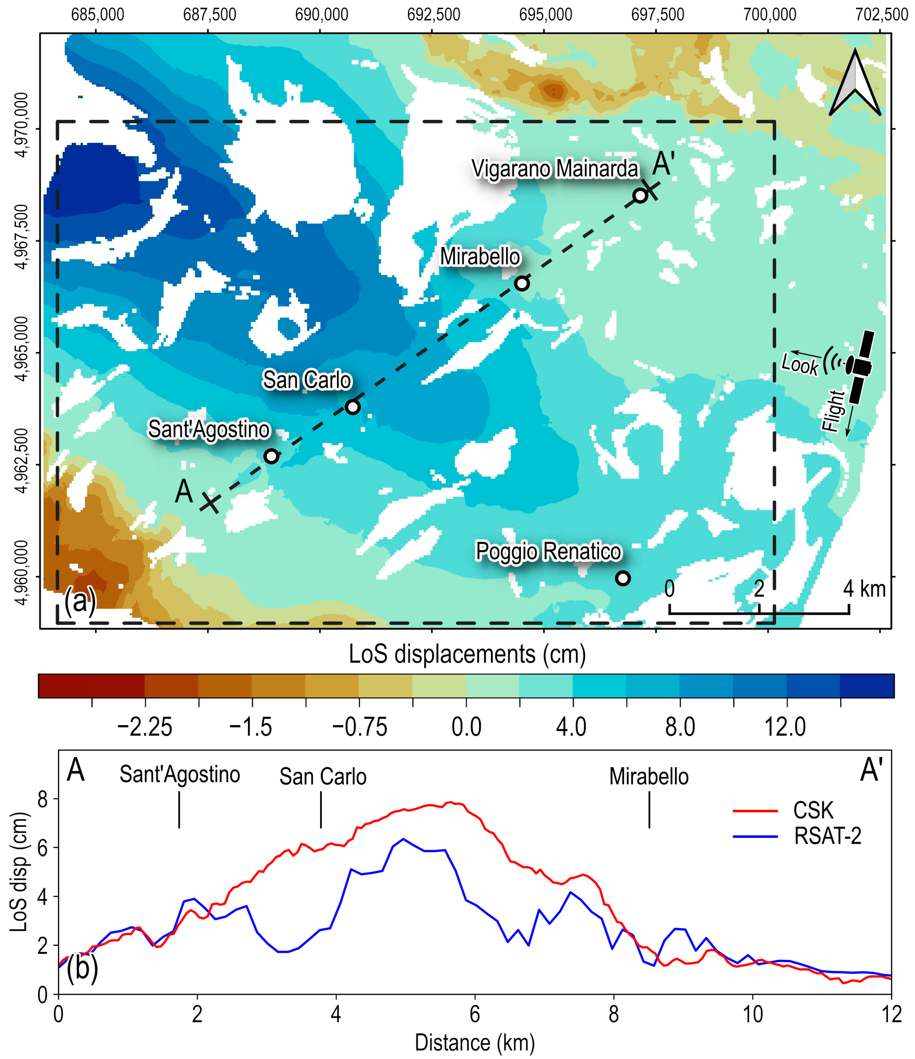
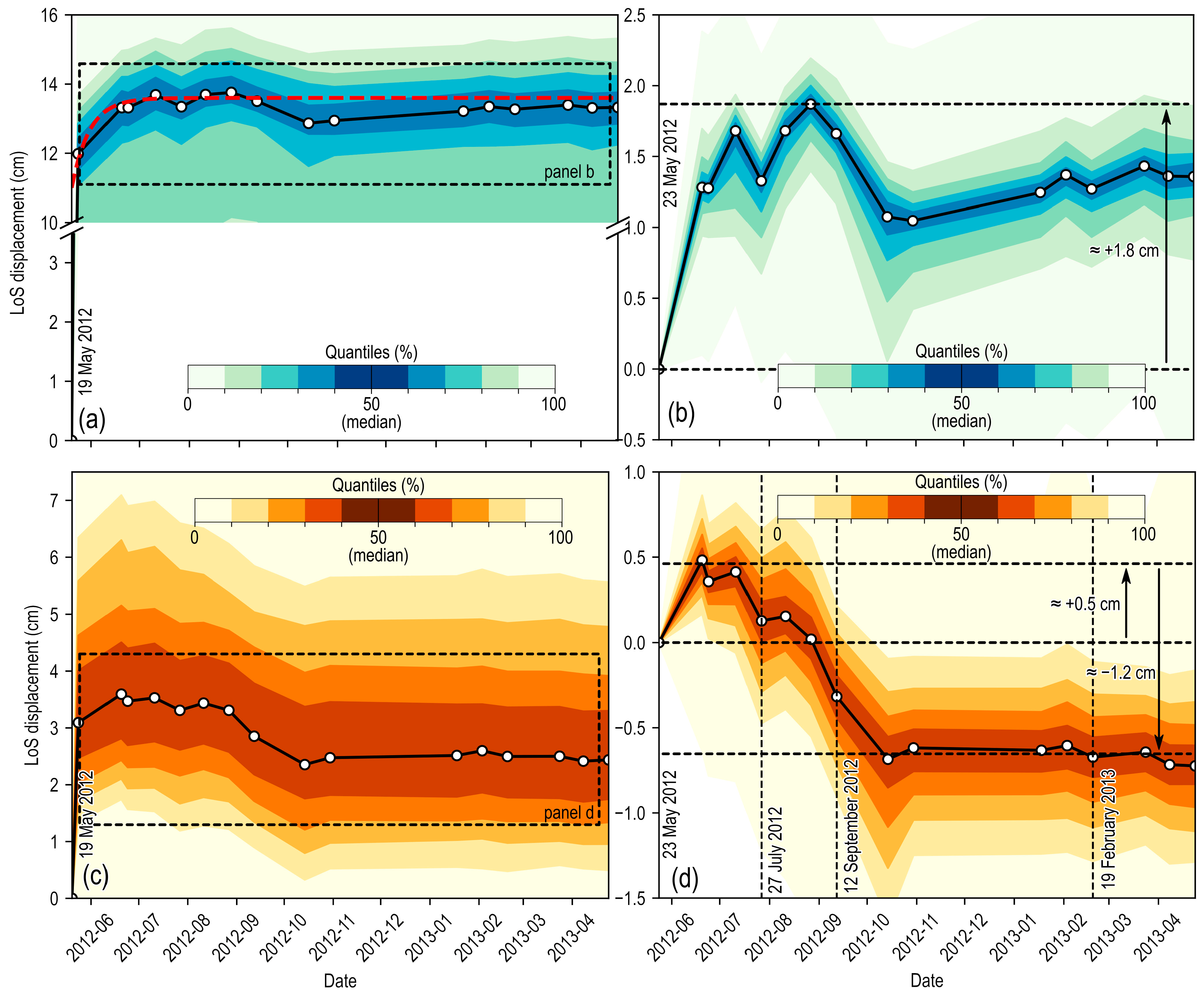
4.1. InSAR-Derived Ground Displacements

The InSAR-derived LoS displacement map of the SAR data acquired on 19–23 May 2012 (Figure 3a) encompasses the coseismic (i.e., almost instantaneous) ground displacements caused by the 20 May 2012 event and the first three days of postseismic ground displacements (from 20 to 23 May). The map highlights ground movements directed mainly toward the satellite sensor (positive values in Figure 3a). Such movements result from the coseismic slip of the Ferrara thrust during the May 20 event, which caused predominant ground uplift because of the reverse focal mechanism [26]. Although the obtained displacement lobe partially images the extent of the deformed area, it reasonably matches the coseismic displacement pattern obtained from the RSAT-2 SAR images in Figure 1 [29,30]. The latter are acquired along the same orbit and with a similar side-looking angle of the CSK SAR data, thus allowing a direct comparison of the ground displacements, as shown in Figure 3b.
In particular, some discrepancies between the CSK and RSAT-2 displacements occurred by looking at the LoS displacement profile over the A–A’ cross-section in Figure 3b. The CSK data showed larger LoS displacements concerning the RSAT-2 data between the Sant’Agostino, San Carlo, and Mirabello villages. Considering that the RSAT-2 displacements incorporated both the coseismic displacements and approximately 29 days of postseismic displacements, we argue that the observed displacement deficit could be ascribable to local ground subsidence that occurred between 23 May and 17 June 2012, which corresponds to the second SAR image acquisitions of the CSK and RSAT-2 data, respectively.
After the 20 May 2012 mainshock, the cumulative LoS displacements from the CSK data on 27 July 2012 (Figure 4a), 12 September 2012 (Figure 4b), and 19 February 2013 (Figure 4c) encompass the entire post-seismic phase starting from 23 May and show that the investigated area underwent a complex deformation pattern.
In the northwestern sector (dotted area in Figure 4a–c), the main lobe of positive LoS displacements represents ground movements toward the satellite sensor.
Otherwise, the area between the S. Agostino and Mirabello villages shows negative LoS displacements, indicating ground movements away from the satellite sensor and amplitudes progressively increasing (in absolute terms) over time (Figure 4a–c). The movements are uneven, with some areas showing an initial displacement increase, followed by a progressive reduction, and some others showing a continuous displacement decline, as observed along the A–A’ cross-section in Figure 4d, crossing the Sant’Agostino, San Carlo, and Mirabello villages (see the trace of the cross-section in Figure 4a–c).
The area’s displacement trends are clear when looking at the time series of DTs (Figure 5). The DTs in the epicentral area to the northwest (the dotted area in Figure 4a–c) show an initial fast increase because of the coseismic fault slip, reaching median LoS displacements of approximately +12 cm and maximum values up to +17 cm (Figure 5a). A further increase in LoS displacements occurs in the postseismic phase, with median values of approximately +1.8 cm (Figure 5b) and maximum values up to +3.5 cm. The latter accumulates from approximately one to two months after the 20 May 2012 event.
This area is near the zone that experienced the maximum coseismic uplift (see Figure 3a), thus suggesting that the observed postseismic displacements have a tectonic origin. Analytical and numerical models from the literature confirm this hypothesis, as the observed post-seismic ground movements are given by fault afterslip and crustal poroelastic stress changes after the mainshock [26,30,36].
The DTs falling in the gridded area over the Sant’Agostino, San Carlo, and Mirabello villages in Figure 4a–c show a complex displacement trend (Figure 5c). The area is first affected by coseismic uplift, but with a lower amplitude than the epicentral area. Then, starting from 23 May 2012 (i.e., the first available SAR image after the 20 May event), we observed a further LoS displacement increase up to median values of +0.5 cm on 20 June 2012 (Figure 5d), followed by a progressive displacement decline until stabilizing at median values of approximately −0.7 cm (maximum values up to −2 cm) at approximately 4–5 months from the 20 May event, while the total median displacement decline, considering the early increase, was approximately −1.2 cm.

4.2. Identification and Estimation of Displacement Sources

The observed postseismic displacement patterns indicate the presence of at least two deformation sources acting in the area, producing ground displacements over time but with different amplitudes and opposite signings. We postulate that the first deformation source is related to the same postseismic tectonic processes affecting the epicentral area to the northwest (i.e., afterslip and poroelastic stress changes), with the Sant’Agostino–Mirabello area also being affected by non-negligible coseismic ground displacements.
Otherwise, widespread liquefaction evidence was observed after the main shock (red circles in Figure 4a–c). Such evidence, which often manifests at the surface with sand boils and water leaks from cracks, indicates the presence of liquefied layers at depth. These layers are also responsible for diffuse ground subsidence, not only during the earthquake shaking, but also in the following days to months because of the slow dissipation of excess pore pressure generated in the deeper layers by the earthquake [12].
Liquefaction-induced ground displacements accumulate not only in places where liquefaction effects manifest on the ground, but also in places where the liquefaction phenomena are not recognized, as this depends on the area’s alluvial stratigraphic architecture [41,67]. Therefore, we assume that the second deformation source could be related to widespread post-liquefaction ground subsidence.
According to the above assumptions, we hypothesize that almost all the observed LoS displacements result from vertical ground movements. Thus, we converted the LoS displacement time series in Figure 5d into equivalent vertical movements according to Equation (2). Then, we assumed that both the postseismic tectonic uplift and the liquefaction-induced consolidation trends follow an exponential decay, as shown in Equation (15):
d = d 0 ± a 1 e t b   ,
where d0 is a fixed displacement term, t is the time, and the a and b terms control the amplitude and shape of the exponential function, respectively. The ± symbol at the second member of Equation (15) is intended to simulate the exponential postseismic uplift (plus symbol) and the postseismic subsidence (minus symbol), respectively.
The algebraic sum of the tectonic and post-liquefaction ground movements should provide the observed median ground displacements retrieved by InSAR and represented in Figure 5c,d with a black line. Therefore, we calibrated the Equation (15) coefficients for tectonic uplift and post-liquefaction subsidence to best reproduce such displacements.
The performed procedure provides the curves in Figure 6, where the green curve represents the theoretical coseismic and postseismic uplift of tectonic origin (U in Figure 6), the blue curve represents the ground subsidence (S in Figure 6), and the yellow curve is the sum of both the green and blue curves (U + S in Figure 6). The latter reasonably mimics the observed vertical displacements (dashed black line in Figure 6), with a mean absolute error (MAE) of approximately 0.38 cm. Figure 6 also reports the coefficients of Equation (15) for both tectonic uplift and post-liquefaction subsidence. For the post-seismic tectonic uplift, the coefficient b (=11 days) in Equation (15) was calibrated by fitting the post-seismic ground uplift observed in the epicentral area, as shown in Figure 5a.
An asymptotic median consolidation subsidence of roughly −2.1 cm is representative of the investigated area, with a consolidation time of approximately 100–150 days.

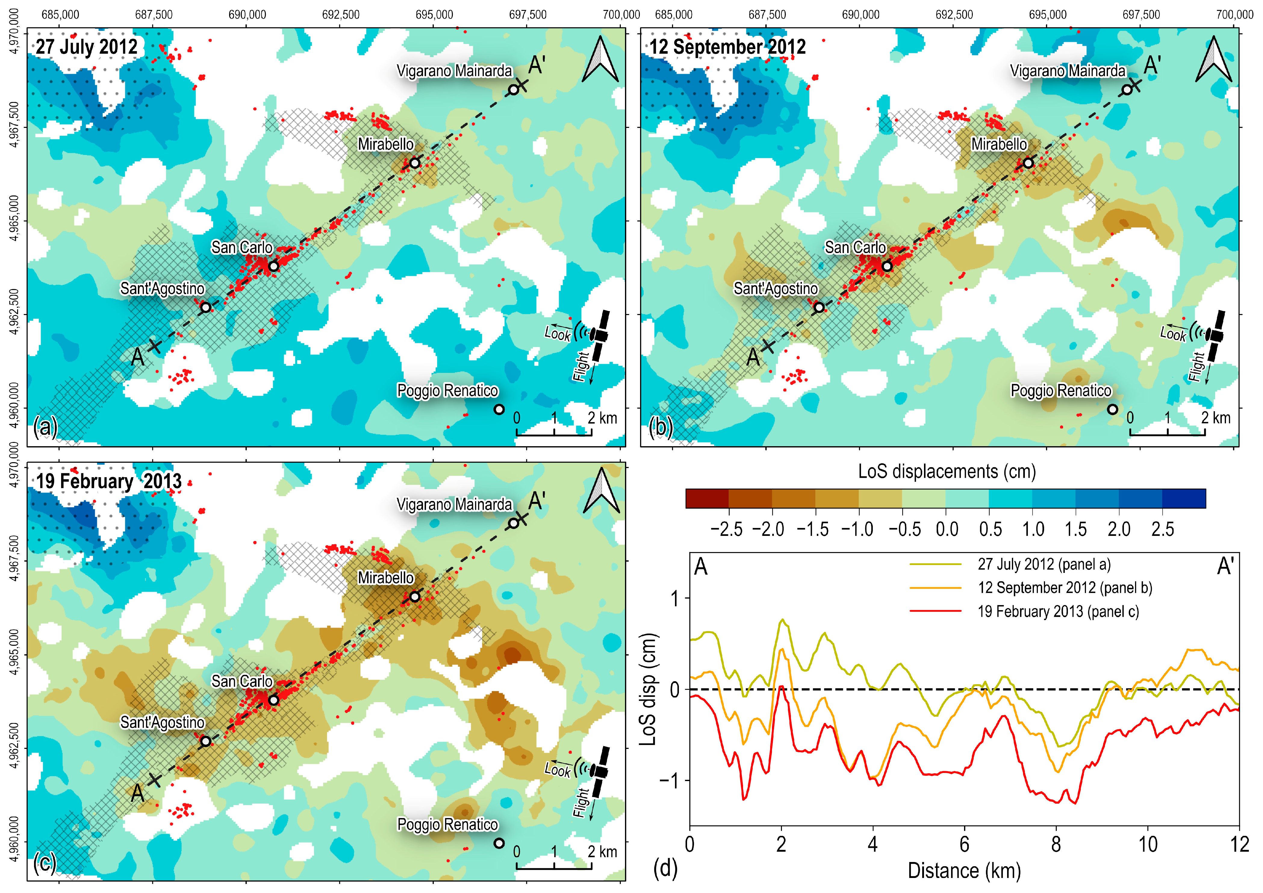
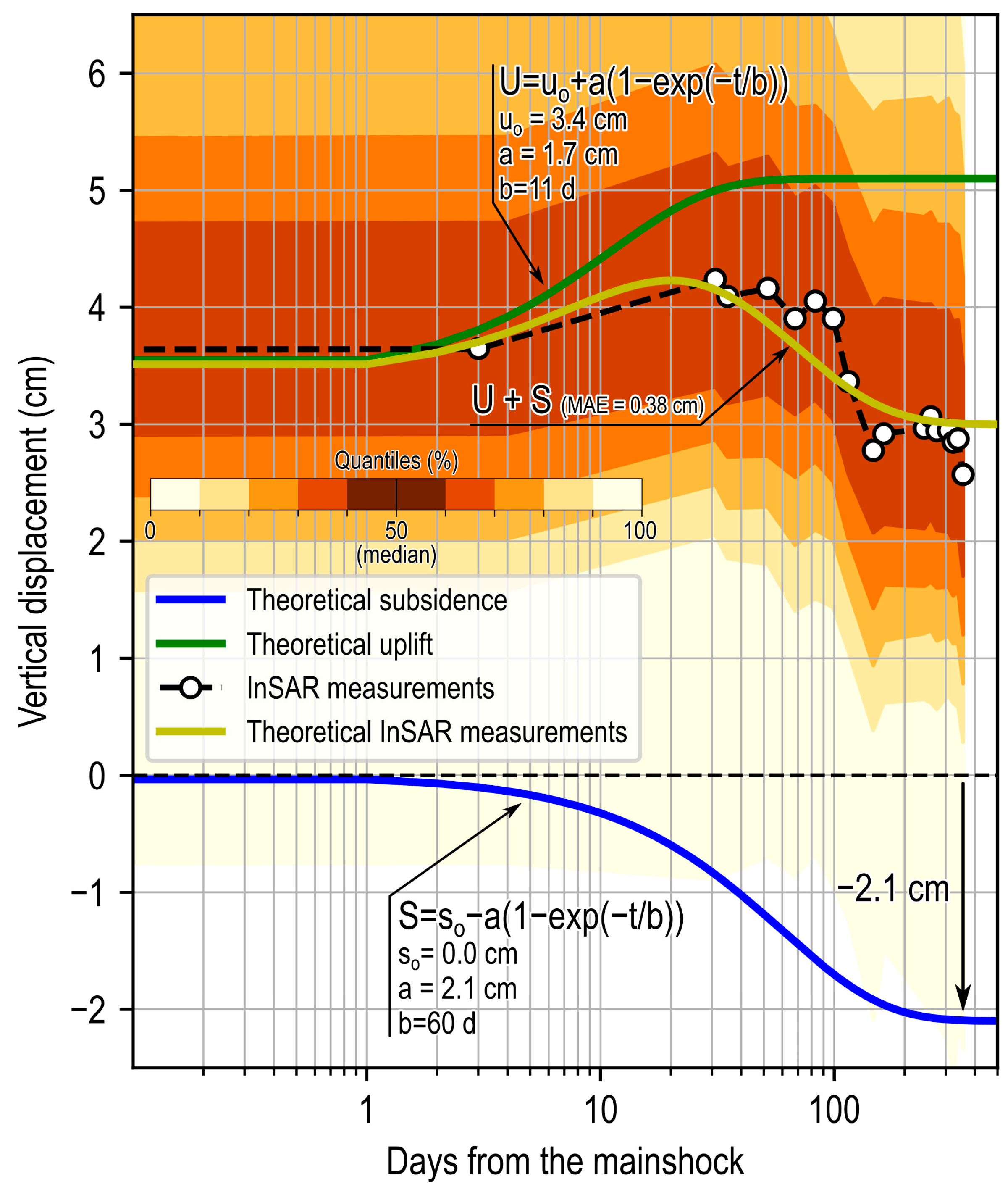
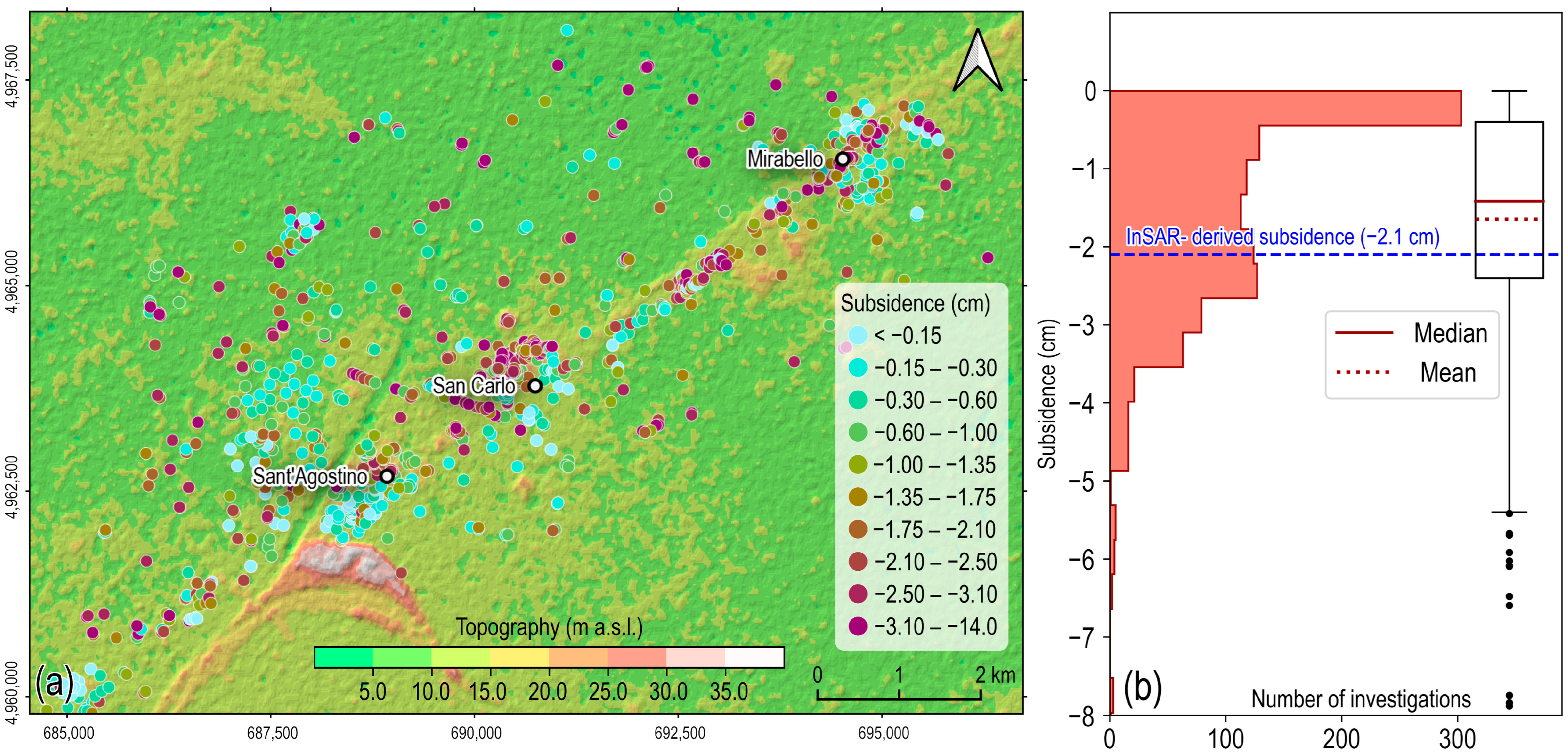
4.3. Estimation of the Post-Liquefaction Consolidation Subsidence

The phenomenon behind the observed post-seismic subsidence was investigated by calculating the post-liquefaction consolidation subsidence according to the procedure described in Section 3.2, implemented in Python code, and applied to all the available cone penetration tests over the study area.
The results revealed a significant spatially heterogeneous distribution of post-liquefaction consolidation subsidence (Figure 7a). This distribution, with larger values often located in proximity to liquefaction evidence at the ground, but also in areas where liquefaction evidence at the ground was not observed, is a key finding. From a spatial point of view, the computed punctual values differ from the InSAR-derived ground subsidence, as shown in Figure 7a. However, some similarities arise when looking at the statistical distribution of the calculated values.
The histogram of the calculated post-liquefaction consolidation subsidence (Figure 7b) is positively skewed. Many of the available cone penetration tests provide vertical movements lower than −0.5 cm. However, most surveys identify subsidence values between −0.4 cm and −2.3 cm, corresponding to the first and third quartile of the distribution of the computed values, respectively, with a mean value of −1.65 cm, slightly larger than its median value (−1.42 cm). This subsidence interval also includes the asymptotic median post-liquefaction subsidence value estimated from the analysis of InSAR data, as shown in Figure 6 (i.e., −2.1 cm as in Figure 6). Such a result highlights that the observed ground displacements are compatible with the estimated consolidation subsidence and provides further evidence about the cause of the observed displacements, which can be attributable to post-liquefaction consolidation.

5. Discussion

The analysis of SAR data over the San Carlo–Mirabello area during the 2012 Emilia seismic sequence identified local ground movements. We argued that such displacements originated from at least two different sources: (i) a regional tectonic source, associated with postseismic fault afterslip and poroelastic stress changes [26,30], and (ii) a shallow ground consolidation source, associated with the post-liquefaction progressive dissipation of excess pore water pressure developed in the saturated sandy layers during earthquake shaking.
The assumed simple exponential decay for both phenomena (Figure 6) allowed us to discriminate between the two contributions to the observed ground displacements, thus providing a simple estimation of a median consolidation subsidence curve, with a maximum subsidence of approximately −2.1 cm and a decay of roughly 4 to 5 months. The ground sinking followed a non-linear and exponential decay trend, which is typical of consolidation processes. It mainly occurred near the area that manifested the effect of liquefaction at the surface and had minimal impact on areas farther away.
Calculating the consolidation subsidence from the available geotechnical database with simple analytical formulations provided a statistical distribution of post-liquefaction ground subsidence, as shown in Figure 7b. The median subsidence estimated from InSAR data (≈−2.1 cm) fell within the first and third percentile of the computed subsidence distribution, slightly larger than the computed median and mean consolidation values. This result supports the hypothesis that the observed subsidence could be attributed to post-liquefaction consolidation subsidence.

5.1. Other Potential Factors Producing Ground Subsidence

Other factors besides post-liquefaction consolidation could cause ground subsidence, such as seasonal changes in aquifers and natural ground subsidence. We ruled out any impact of changes in the groundwater table on the observed ground sinking by looking at the depth of groundwater levels from multiple wells near the study area, as depicted in Figure S3a (data available from: https://www.arpae.it/it/temi-ambientali/acqua/dati-acque/acque-sotterranee, accessed on 3 June 2024). Even if the sampling rate was not perfect, we did not see clear signs of prolonged groundwater depletion in the first 200 m depth from 2010 to 2015 (Figure S3b). Therefore, we can infer that the observed ground subsidence was not linked to changes in the groundwater table.
Regarding natural ground subsidence, InSAR displacement time series data from the ENVISAT satellite constellation, covering the period 2003–2010 and available from the Italian Ministry of the Environment, Earth and Sea [68], show the potential ground subsidence in the area before the earthquake sequence (Figure S4). The area experienced linear displacement rates of approximately −2 mm per year along ascending (Figure S4a) and descending (Figure S4b) orbits, with maximum values reaching −3–−4 mm per year at a few locations. Vertical and east–west horizontal displacement rates (Figure S4c and d, respectively) obtained by combining the ascending and descending orbits [69] showed similar amplitudes and did not reveal any significant pattern over the investigated area. Therefore, these displacement rates are compatible with the natural consolidation subsidence, as in Carminati and Di Donato [70], and are considered negligible in the context of the observed ground subsidence during the 2012 earthquake sequence.

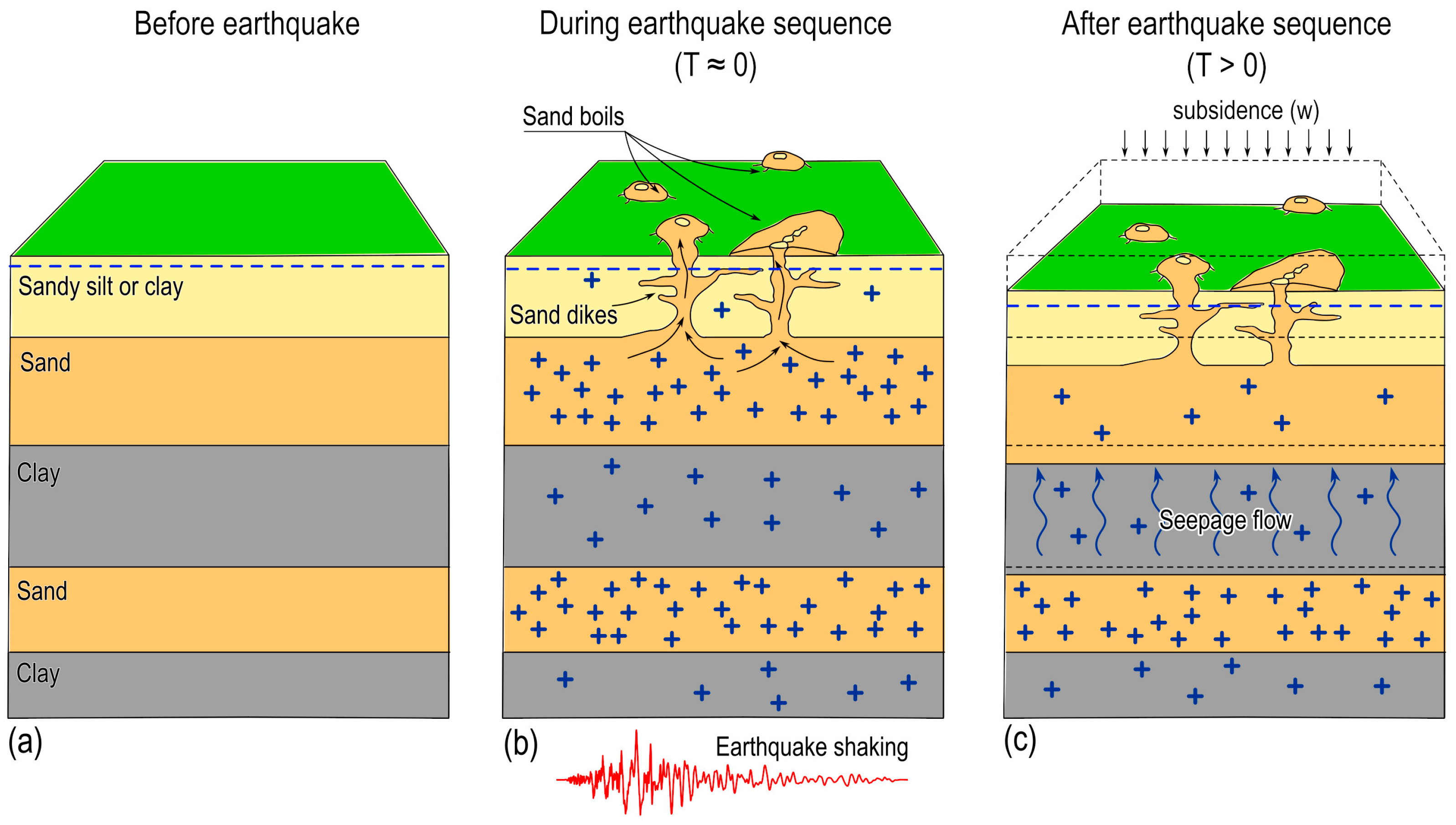
5.2. Conceptual Scheme of the Observed Phenomenon

Considering our results, we proposed a simple explicatory scheme, as shown in Figure 8, to support our conclusions about the observed displacements and further discuss the time delay in the consolidation process.
Based on the typical geotechnical cross-section shown in Figure 2, we represented the stratigraphic column of the first 30 m of the study area in Figure 8a. The seismic shaking during the earthquake sequence led to excess pore pressure (depicted by the blue plus symbols in Figure 8b), which caused liquefaction of the saturated sandy layers. Our working assumption is that the arrangement of the main architectural elements of the alluvial succession below the groundwater table depth determines whether liquefaction may occur in the field.
The liquefaction of the shallower sandy layers, especially those located within or below the braided paleo-drainages and abandoned meanders, had widespread effects on the ground, such as sand boils and water leaks from cracks. This was also accompanied by nearly instantaneous local subsidence (Figure 8b) [13,31]. Excess pore pressures caused an upward flow of a sufficient volume and speed to lift soil particles and carry them to the ground surface. As a result, the pore water typically found or created cracks or holes through which it could flow to the surface. Indeed, the distribution of liquefaction effects seemed aligned with channel–levee complexes and is associated with prominent geomorphological features or lateral spreading effects in the study area [8,31].
The absence of sand ejecta in other areas does not mean that sandy layers at depth did not liquefy. According to Kramer et al. [67], if the top of the liquefied layer is too deep, sand boils will not form, even if liquefaction below the crust does occur, because the upper, non-liquefiable layer is too thick. Therefore, we expect that liquefaction occurred also in the deep sand layer, as shown in Figure 8b [8]. For these layers, which are confined between thick clay deposits [41,42], the pore water pressure dissipation is not as fast as the shallower layers, but is governed by the in-series seepage flow across both sandy and clay-like layers. The speed of in-series groundwater flow and pore pressure dissipation is governed mainly by the layer with the lowest permeability, which, in this case, is represented by the clay-like layer, characterized by low permeabilities of the order of k = 2–3 × 10⁻⁹ cm/s [40]. Such behavior could explain the approximately 4- to 5-month timespan required to achieve asymptotic subsidence.
Consequently, a slow consolidation process developed, with a progressive displacement accumulation over time (Figure 8c). Other strong aftershocks during the seismic sequence could have also enhanced excess pore pressures [40], even producing new liquefaction effects at the ground (e.g., sand ejecta) and re-liquefaction at some sites [38], thus extending the pore pressure dissipation time.
The observed ground displacements from the InSAR analysis confirm the proposed scheme, since the observed ground subsidence manifested independently at the location of liquefaction-related manifestations at the ground (Figure 4). Moreover, the amplitude of the observed displacements was compatible with the computed consolidation values, thus providing further confirmation about the origin of the post-liquefaction consolidation of the observed ground movements.

5.3. Uncertainties and Further Developments

It is worth analyzing the uncertainties related to the obtained results. In particular, the InSAR-derived theoretical consolidation curve, as shown in Figure 6, was obtained by averaging the InSAR observations over the study area and assuming some simplified behavior for the involved phenomena. The calculation of the estimated statistical distribution of consolidation subsidence was also affected by several uncertainties, as it was based on a simplified analytical approach. Finally, the dissipation time of excess pore pressure was strictly dependent on the assumed boundary conditions, which were related to the geomorphological setting of the subsoil of the study area. The main limitation in the boundary conditions adopted in this study was the hypothesis of one-dimensional consolidation. Indeed, the drainage path followed by the water was tridimensional and particularly deviated from the vertical assumption when elements working as “vent valves” were present, e.g., wells. Better results should be obtained in estimating consolidation values over time with more sophisticated methods, such as numerical analysis, which better models the development of liquefaction and dissipation of excess pore pressure, potentially yielding more accurate displacement estimates [12,40]. However, there is a tradeoff between the complexity of the analysis and the effort needed to acquire input parameters. According to the spatial extent and complexity of the study area, the adopted approach provided a reasonable estimate of post-liquefaction subsidence, and it was adequate to explain the observed phenomenon at a regional scale. More detailed numerical analyses can be performed, but at a larger scale than that adopted in this study, since they require detailed knowledge of the subsoil’s geometrical and lithological features.

6. Conclusions

In this work, the analysis of the InSAR displacement time series during the Emilia 2012 seismic sequence allowed, for the first time, to observe the evolution over time of post-liquefaction consolidation subsidence over the San Carlo, Sant’Agostino, and Mirabello villages, which have been affected by widespread liquefaction evidence at the ground. We argued that the observed subsidence is associated with the slow pore pressure dissipation of a deep and almost spatially continuous sandy layer, which liquefied during the seismic sequence and whose consolidation is mainly governed by seepage flow across clayey upper layers to the top. Such a hypothesis is corroborated by the fact that the observed subsidence localizes in areas with liquefaction evidence at the ground and also spreads over areas where direct evidence of deep liquefaction has not been identified, as it is related to the consolidation of deeper and spatially continuous sandy strata. The observed ground displacements from the InSAR analysis confirm the proposed scheme, since the observed ground subsidence manifested independently at the location of liquefaction-related manifestations at the ground. Moreover, the amplitude of the observed displacements is compatible with the computed consolidation values, thus providing further confirmation about the origin of the post-liquefaction consolidation of the observed ground movements.

Supplementary Materials

The following supporting information can be downloaded at: https://www.mdpi.com/article/10.3390/rs16132364/s1, Figure S1. Spatial and temporal baseline distribution of the CSK data set. The data set begins 1 day before the 20 May 2012 main shock and includes ≈150 days of postseismic deformation. The lines between the different acquisitions define the interferometric pairs used for construction of the SBAS time series. Figure S2: (a) Spatial distribution of the available geotechnical investigations over the study area (from Varone et al. [60]). (b) Boxplot of the computed maximum PGA over the study area (from Papathanassiou et al. [42]). (c) Experimental shear modulus reduction curves from resonant column tests (from Sinatra and Foti [40]), together with the theoretical curve defined according to Equation (14) [66]. Figure S3. (a) Location of the available groundwater wells in the study area, classified according to their maximum depth (data available from: https://www.arpae.it/it/temi-ambientali/acqua/dati-acque/acque-sotterranee, accessed on 3 June 2024). (b) Measured groundwater depth from the ground at water wells in panel (a). Figure S4. Mean InSAR displacement rate maps in the period 2003–2010 from ENVISAT SAR data, computed along the (a) ascending and (b) descending satellite orbit acquisitions. Panels c and d show the vertical and the east-west horizontal components of the displacement rate, obtained by combining the ascending (a) and descending (b) displacement rates.

Author Contributions

Conceptualization, M.A. and A.C.; data curation, A.P. and G.S.; formal analysis, M.A., A.P. and G.S.; investigation, M.S. and M.M.; methodology, M.A. and A.C.; software, M.A., A.P. and G.S.; validation, A.C., M.S. and M.M.; visualization, M.A.; writing—original draft, M.A.; writing—review and editing, A.C., M.S., M.M., A.P. and G.S. All authors have read and agreed to the published version of the manuscript.

Funding

This research received no external funding.

Data Availability Statement

The raw data supporting the conclusions of this article will be made available by the authors upon request.

Acknowledgments

We thank the Italian Space Agency for providing the CSK SAR data. Scientific color maps [71] are used in this study to prevent visual distortion of the data and exclusion of readers with color-vision deficiencies. The Geology and Geotechnologies Laboratory (INGV, https://www.ingv.it/monitoraggio-e-infrastrutture/laboratori/laboratorio-geologia-e-geotecnologia) provided the ENVISAT PS DInSAR dataset in the framework of an agreement with the Ministry of the Environment, Earth and Sea (http://www.pcn.minambiente.it)—Italian National Geoportal, owner of the data.

Conflicts of Interest

The authors declare no conflicts of interest.

References

  1. Obermeier, S.F. The New Madrid Earthquakes: An Engineering-Geologic Interpretation of Relict Liquefaction Features; Professional Paper; United States Government Printing Office: Washington, DC, USA, 1989. [Google Scholar]
  2. Seed, H.B. The Fourth Terzaghi Lecture: Landslides during Earthquakes Due to Liquefaction. J. Soil Mech. Found. Div. 1968, 94, 1053–1122. [Google Scholar] [CrossRef]
  3. Seed, H.B.; Idriss, I.M. Analysis of Soil Liquefaction: Niigata Earthquake. J. Soil Mech. Found. Div. 1967, 93, 83–108. [Google Scholar] [CrossRef]
  4. Sonmez, B.; Ulusay, R.; Sonmez, H. A Study on the Identification of Liquefaction-Induced Failures on Ground Surface Based on the Data from the 1999 Kocaeli and Chi-Chi Earthquakes. Eng. Geol. 2008, 97, 112–125. [Google Scholar] [CrossRef]
  5. Wang, C.; Dreger, D.S.; Wang, C.; Mayeri, D.; Berryman, J.G. Field Relations among Coseismic Ground Motion, Water Level Change and Liquefaction for the 1999 Chi-Chi (Mw = 7.5) Earthquake, Taiwan. Geophys. Res. Lett. 2003, 30, 2003GL017601. [Google Scholar] [CrossRef]
  6. Elgamal, A.-W.; Zeghal, M.; Parra, E. Liquefaction of Reclaimed Island in Kobe, Japan. J. Geotech. Engrg. 1996, 122, 39–49. [Google Scholar] [CrossRef]
  7. Quigley, M.C.; Bastin, S.; Bradley, B.A. Recurrent Liquefaction in Christchurch, New Zealand, during the Canterbury Earthquake Sequence. Geology 2013, 41, 419–422. [Google Scholar] [CrossRef]
  8. Minarelli, L.; Amoroso, S.; Civico, R.; De Martini, P.M.; Lugli, S.; Martelli, L.; Molisso, F.; Rollins, K.M.; Salocchi, A.; Stefani, M.; et al. Liquefied Sites of the 2012 Emilia Earthquake: A Comprehensive Database of the Geological and Geotechnical Features (Quaternary Alluvial Po Plain, Italy). Bull Earthq. Eng 2022, 20, 3659–3697. [Google Scholar] [CrossRef]
  9. Jalil, A.; Fathani, T.F.; Satyarno, I.; Wilopo, W. Liquefaction in Palu: The Cause of Massive Mudflows. Geoenviron. Disasters 2021, 8, 21. [Google Scholar] [CrossRef]
  10. Kramer, S.L. Geotechnical Earthquake Engineering; Prentice-Hall international series in civil engineering and engineering mechanics; Prentice Hall: Upper Saddle River, NJ, USA, 1996; ISBN 978-0-13-374943-4. [Google Scholar]
  11. Zeybek, A.; Madabhushi, G.S.P. Assessment of Soil Parameters during Post-Liquefaction Reconsolidation of Loose Sand. Soil Dyn. Earthq. Eng. 2023, 164, 107611. [Google Scholar] [CrossRef]
  12. Chiaradonna, A.; d’Onofrio, A.; Bilotta, E. Assessment of Post-Liquefaction Consolidation Settlement. Bull. Earthq. Eng. 2019, 17, 5825–5848. [Google Scholar] [CrossRef]
  13. Chini, M.; Albano, M.; Saroli, M.; Pulvirenti, L.; Moro, M.; Bignami, C.; Falcucci, E.; Gori, S.; Modoni, G.; Pierdicca, N.; et al. Coseismic Liquefaction Phenomenon Analysis by COSMO-SkyMed: 2012 Emilia (Italy) Earthquake. Int. J. Appl. Earth Obs. Geoinf. 2015, 39, 65–78. [Google Scholar] [CrossRef]
  14. Dashti, S.; Bray, J.D.; Pestana, J.M.; Riemer, M.; Wilson, D. Mechanisms of Seismically Induced Settlement of Buildings with Shallow Foundations on Liquefiable Soil. J. Geotech. Geoenviron. Eng. 2010, 136, 151–164. [Google Scholar] [CrossRef]
  15. Adamidis, O.; Madabhushi, S.P.G. Deformation Mechanisms under Shallow Foundations on Liquefiable Layers of Varying Thickness. Géotechnique 2017, 68, 602–613. [Google Scholar] [CrossRef]
  16. Albano, M.; Saroli, M.; Beccaro, L.; Moro, M.; Doumaz, F.; Discenza, M.E.; Del Rio, L.; Rompato, M. Multi-Source Data Analysis to Assess the Past and Present Kinematics of the Pisciotta Deep-Seated Gravitational Slope Deformation (Southern Italy). Remote Sens. Environ. 2023, 296, 113751. [Google Scholar] [CrossRef]
  17. Li, S.; Xu, W.; Li, Z. Review of the SBAS InSAR Time-Series Algorithms, Applications, and Challenges. Geod. Geodyn. 2022, 13, 114–126. [Google Scholar] [CrossRef]
  18. Lundgren, P.; Casu, F.; Manzo, M.; Pepe, A.; Berardino, P.; Sansosti, E.; Lanari, R. Gravity and Magma Induced Spreading of Mount Etna Volcano Revealed by Satellite Radar Interferometry. Geophys. Res. Lett. 2004, 31, 2003GL018736. [Google Scholar] [CrossRef]
  19. Beccaro, L.; Albano, M.; Tolomei, C.; Spinetti, C.; Pezzo, G.; Palano, M.; Chiarabba, C. Insights into Post-Emplacement Lava FLow Dynamics at Mt. Etna Volcano from 2016 to 2021 by Synthetic Aperture Radar and Multispectral Satellite Data. Front. Earth Sci. 2023, 11, 14. [Google Scholar] [CrossRef]
  20. Stramondo, S.; Trasatti, E.; Albano, M.; Moro, M.; Chini, M.; Bignami, C.; Polcari, M.; Saroli, M. Uncovering Deformation Processes from Surface Displacements. J. Geodyn. 2016, 102, 58–82. [Google Scholar] [CrossRef]
  21. Pousse-Beltran, L.; Socquet, A.; Benedetti, L.; Doin, M.; Rizza, M.; D’Agostino, N. Localized Afterslip at Geometrical Complexities Revealed by InSAR After the 2016 Central Italy Seismic Sequence. JGR Solid Earth 2020, 125, e2019JB019065. [Google Scholar] [CrossRef]
  22. Moro, M.; Saroli, M.; Stramondo, S.; Bignami, C.; Albano, M.; Falcucci, E.; Gori, S.; Doglioni, C.; Polcari, M.; Tallini, M.; et al. New Insights into Earthquake Precursors from InSAR. Sci. Rep. 2017, 7, 12035. [Google Scholar] [CrossRef]
  23. Cando-Jácome, M.; Martínez-Graña, A.; Chunga, K.; Ortíz-Hernández, E. Satellite Radar Interferometry for Assessing Coseismic Liquefaction in Portoviejo City, Induced by the Mw 7.8 2016 Pedernales, Ecuador Earthquake. Environ. Earth Sci. 2020, 79, 467. [Google Scholar] [CrossRef]
  24. Barnhart, W.D.; Yeck, W.L.; McNamara, D.E. Induced Earthquake and Liquefaction Hazards in Oklahoma, USA: Constraints from InSAR. Remote Sens. Environ. 2018, 218, 1–12. [Google Scholar] [CrossRef]
  25. Fujiwara, S.; Nakano, T.; Morishita, Y.; Kobayashi, T.; Yarai, H.; Une, H.; Hayashi, K. Detection and Interpretation of Local. Surface Deformation from the 2018 Hokkaido Eastern Iburi Earthquake Using ALOS-2 SAR Data. Earth Planets Space 2019, 71, 64. [Google Scholar] [CrossRef]
  26. Cheloni, D.; Giuliani, R.; D’Agostino, N.; Mattone, M.; Bonano, M.; Fornaro, G.; Lanari, R.; Reale, D.; Atzori, S. New Insights into Fault Activation and Stress Transfer between en Echelon Thrusts: The 2012 Emilia, Northern Italy, Earthquake Sequence. JGR Solid Earth 2016, 121, 4742–4766. [Google Scholar] [CrossRef]
  27. Govoni, A.; Marchetti, A.; De Gori, P.; Di Bona, M.; Lucente, F.P.; Improta, L.; Chiarabba, C.; Nardi, A.; Margheriti, L.; Agostinetti, N.P.; et al. The 2012 Emilia Seismic Sequence (Northern Italy): Imaging the Thrust Fault System by Accurate Aftershock Location. Tectonophysics 2014, 622, 44–55. [Google Scholar] [CrossRef]
  28. Scognamiglio, L.; Margheriti, L.; Mele, F.M.; Tinti, E.; Bono, A.; De Gori, P.; Lauciani, V.; Lucente, F.P.; Mandiello, A.G.; Marcocci, C.; et al. The 2012 Pianura Padana Emiliana Seimic Sequence: Locations, Moment Tensors and Magnitudes. Ann. Geophys. 2012, 55, 5. [Google Scholar] [CrossRef]
  29. Tizzani, P.; Castaldo, R.; Solaro, G.; Pepe, S.; Bonano, M.; Casu, F.; Manunta, M.; Manzo, M.; Pepe, A.; Samsonov, S.; et al. New Insights into the 2012 Emilia (Italy) Seismic Sequence through Advanced Numerical Modeling of Ground Deformation InSAR Measurements. Geophys. Res. Lett. 2013, 40, 1971–1977. [Google Scholar] [CrossRef]
  30. Albano, M.; Barba, S.; Solaro, G.; Pepe, A.; Bignami, C.; Moro, M.; Saroli, M.; Stramondo, S. Aftershocks, Groundwater Changes and Postseismic Ground Displacements Related to Pore Pressure Gradients: Insights from the 2012 Emilia-Romagna Earthquake: The 2012 Emilia-Romagna Earthquake. J. Geophys. Res. Solid Earth 2017, 122, 5622–5638. [Google Scholar] [CrossRef]
  31. Emergeo Working Group Liquefaction Phenomena Associated with the Emilia Earthquake Sequence of May–June 2012 (Northern Italy). Nat. Hazards Earth Syst. Sci. 2013, 13, 935–947. [CrossRef]
  32. Martelli, L.; Nardi, G.; Cavuoto, G.; Conforti, A.; Ferraro, L.; D’Argenio, B. Note Illustrative Della Carta Geologica d’Italia Alla Scala 1:50.000; Foglio 519 Capo Palinuro; Istituto Superiore per la Protezione e la Ricerca Ambientale: Regione Campania, Italy, 2016. [Google Scholar]
  33. Ghielmi, M.; Minervini, M.; Nini, C.; Rogledi, S.; Rossi, M.; Vignolo, A. Sedimentary and Tectonic Evolution in the Eastern Po-Plain and Northern Adriatic Sea Area from Messinian to Middle Pleistocene (Italy). Rend. Fis. Acc. Lincei 2010, 21, 131–166. [Google Scholar] [CrossRef]
  34. Marcaccio, M.; Martinelli, G. Effects on the Groundwater Levels of the May–June 2012 Emilia Seismic Sequence. Ann. Geophys. 2012, 55, 38. [Google Scholar] [CrossRef]
  35. Nespoli, M.; Todesco, M.; Serpelloni, E.; Belardinelli, M.E.; Bonafede, M.; Marcaccio, M.; Rinaldi, A.P.; Anderlini, L.; Gualandi, A. Modeling Earthquake Effects on Groundwater Levels: Evidences from the 2012 Emilia Earthquake (Italy). Geofluids 2016, 16, 452–463. [Google Scholar] [CrossRef]
  36. Nespoli, M.; Belardinelli, M.E.; Gualandi, A.; Serpelloni, E.; Bonafede, M. Poroelasticity and Fluid Flow Modeling for the 2012 Emilia-Romagna Earthquakes: Hints from GPS and InSAR Data. Geofluids 2018, 2018, 15. [Google Scholar] [CrossRef]
  37. Cinti, D.; Sciarra, A.; Cantucci, B.; Galli, G.; Pizzino, L.; Procesi, M.; Poncia, P.P. Hydrogeochemical Investigation of Shallow Aquifers before and after the 2012 Emilia Seismic Sequence (Northern Italy). Appl. Geochem. 2023, 151, 105624. [Google Scholar] [CrossRef]
  38. Di Manna, P.; Guerrieri, L.; Piccardi, L.; Vittori, E.; Castaldini, D.; Berlusconi, A.; Bonadeo, L.; Comerci, V.; Ferrario, F.; Gambillara, R.; et al. Ground Effects Induced by the 2012 Seismic Sequence in Emilia: Implications for Seismic Hazard Assessment in the Po Plain. Ann. Geophys. 2012, 55, 23. [Google Scholar] [CrossRef]
  39. Civico, R.; Brunori, C.A.; De Martini, P.M.; Pucci, S.; Cinti, F.R.; Pantosti, D. Liquefaction Susceptibility Assessment in Fluvial Plains Using Airborne Lidar: The Case of the 2012 Emilia Earthquake Sequence Area (Italy). Nat. Hazards Earth Syst. Sci. 2015, 15, 2473–2483. [Google Scholar] [CrossRef]
  40. Sinatra, L.; Foti, S. The Role of Aftershocks in the Liquefaction Phenomena Caused by the Emilia 2012 Seismic Sequence. Soil Dyn. Earthq. Eng. 2015, 75, 234–245. [Google Scholar] [CrossRef]
  41. Tentori, D.; Mancini, M.; Varone, C.; Spacagna, R.; Baris, A.; Milli, S.; Gaudiosi, I.; Simionato, M.; Stigliano, F.; Modoni, G.; et al. The Influence of Alluvial Stratigraphic Architecture on Liquefaction Phenomena: A Case Study from the Terre Del Reno Subsoil (Southern Po Plain, Italy). Sediment. Geol. 2022, 440, 106258. [Google Scholar] [CrossRef]
  42. Papathanassiou, G.; Mantovani, A.; Tarabusi, G.; Rapti, D.; Caputo, R. Assessment of Liquefaction Potential for Two Liquefaction Prone Areas Considering the May 20, 2012 Emilia (Italy) Earthquake. Eng. Geol. 2015, 189, 1–16. [Google Scholar] [CrossRef]
  43. Berardino, P.; Fornaro, G.; Lanari, R.; Sansosti, E. A New Algorithm for Surface Deformation Monitoring Based on Small Baseline Differential SAR Interferograms. IEEE Trans. Geosci. Remote Sens. 2002, 40, 2375–2383. [Google Scholar] [CrossRef]
  44. Ferretti, A.; Prati, C.; Rocca, F. Permanent Scatterers in SAR Interferometry. IEEE Trans. Geosci. Remote Sens. 2001, 39, 8–20. [Google Scholar] [CrossRef]
  45. Rosen, P.A.; Hensley, S.; Joughin, I.R.; Li, F.K.; Madsen, S.N.; Rodriguez, E.; Goldstein, R.M. Synthetic Aperture Radar Interferometry. Proc. IEEE 2000, 88, 333–382. [Google Scholar] [CrossRef]
  46. Goldstein, R.M.; Werner, C.L. Radar Interferogram Filtering for Geophysical Applications. Geophys. Res. Lett. 1998, 25, 4035–4038. [Google Scholar] [CrossRef]
  47. Pepe, A.; Lanari, R. On the Extension of the Minimum Cost Flow Algorithm for Phase Unwrapping of Multitemporal Differential SAR Interferograms. IEEE Trans. Geosci. Remote Sens. 2006, 44, 2374–2383. [Google Scholar] [CrossRef]
  48. Casu, F.; Manzo, M.; Lanari, R. A Quantitative Assessment of the SBAS Algorithm Performance for Surface Deformation Retrieval from DInSAR Data. Remote Sens. Environ. 2006, 102, 195–210. [Google Scholar] [CrossRef]
  49. Tizzani, P.; Berardino, P.; Casu, F.; Euillades, P.; Manzo, M.; Ricciardi, G.; Zeni, G.; Lanari, R. Surface Deformation of Long Valley Caldera and Mono Basin, California, Investigated with the SBAS-InSAR Approach. Remote Sens. Environ. 2007, 108, 277–289. [Google Scholar] [CrossRef]
  50. Cheloni, D.; De Novellis, V.; Albano, M.; Antonioli, A.; Anzidei, M.; Atzori, S.; Avallone, A.; Bignami, C.; Bonano, M.; Calcaterra, S.; et al. Geodetic Model of the 2016 Central Italy Earthquake Sequence Inferred from InSAR and GPS Data: Modeling 2016 Central Italy Earthquakes. Geophys. Res. Lett. 2017, 44, 6778–6787. [Google Scholar] [CrossRef]
  51. Manzo, M.; Fialko, Y.; Casu, F.; Pepe, A.; Lanari, R. A Quantitative Assessment of DInSAR Measurements of Interseismic Deformation: The Southern San Andreas Fault Case Study. Pure Appl. Geophys. 2012, 169, 1463–1482. [Google Scholar] [CrossRef]
  52. Pepe, A.; Yang, Y.; Manzo, M.; Lanari, R. Improved EMCF-SBAS Processing Chain Based on Advanced Techniques for the Noise-Filtering and Selection of Small Baseline Multi-Look DInSAR Interferograms. IEEE Trans. Geosci. Remote Sens. 2015, 53, 4394–4417. [Google Scholar] [CrossRef]
  53. Pepe, A.; Calò, F. A Review of Interferometric Synthetic Aperture RADAR (InSAR) Multi-Track Approaches for the Retrieval of Earth’s Surface Displacements. Appl. Sci. 2017, 7, 1264. [Google Scholar] [CrossRef]
  54. Manunta, M.; De Luca, C.; Zinno, I.; Casu, F.; Manzo, M.; Bonano, M.; Fusco, A.; Pepe, A.; Onorato, G.; Berardino, P.; et al. The Parallel SBAS Approach for Sentinel-1 Interferometric Wide Swath Deformation Time-Series Generation: Algorithm Description and Products Quality Assessment. IEEE Trans. Geosci. Remote Sens. 2019, 57, 6259–6281. [Google Scholar] [CrossRef]
  55. Krige, D.G. A Statistical Approach to Some Basic Mine Valuation Problems on the Witwatersrand. J. Chem. Metall. Min. Sociaty S. Afr. 1951, 52, 119–139. [Google Scholar]
  56. Oliver, M.A.; Webster, R. A Tutorial Guide to Geostatistics: Computing and Modelling Variograms and Kriging. CATENA 2014, 113, 56–69. [Google Scholar] [CrossRef]
  57. Saroli, M.; Albano, M.; Modoni, G.; Moro, M.; Milana, G.; Spacagna, R.-L.; Falcucci, E.; Gori, S.; Scarascia Mugnozza, G. Insights into Bedrock Paleomorphology and Linear Dynamic Soil Properties of the Cassino Intermontane Basin (Central Italy). Eng. Geol. 2020, 264, 105333. [Google Scholar] [CrossRef]
  58. Spadi, M.; Tallini, M.; Albano, M.; Cosentino, D.; Nocentini, M.; Saroli, M. New Insights on Bedrock Morphology and Local Seismic Amplification of the Castelnuovo Village (L’Aquila Basin, Central Italy). Eng. Geol. 2022, 297, 106506. [Google Scholar] [CrossRef]
  59. Pebesma, E.J. Multivariable Geostatistics in S: The Gstat Package. Comput. Geosci. 2004, 30, 683–691. [Google Scholar] [CrossRef]
  60. Varone, C.; Carbone, G.; Baris, A.; Caciolli, M.C.; Fabozzi, S.; Fortunato, C.; Gaudiosi, I.; Giallini, S.; Mancini, M.; Paolella, L.; et al. PERL: A Dataset of Geotechnical, Geophysical, and Hydrogeological Parameters for Earthquake-Induced Hazards Assessment in Terre Del Reno (Emilia-Romagna, Italy). Nat. Hazards Earth Syst. Sci. 2023, 23, 1371–1382. [Google Scholar] [CrossRef]
  61. Robertson, P.K. Soil Behaviour Type from the CPT: An Update. In Proceedings of the 2nd International Symposium on Cone Penetration Testing, Huntington Beach, CA, USA, 9–11 May 2010; Volume 2, pp. 575–583. [Google Scholar]
  62. Terzaghi, K. Theoretical Soil Mechanics; John Wiley & Sons, Inc.: Hoboken, NJ, USA, 1943; ISBN 978-0-470-17276-6. [Google Scholar]
  63. Robertson, P.K.; Cabal, K. Guide to Cone Penetration Testing, 7th ed.; Gregg Drilling LLC: Benicia, CA, USA, 2022. [Google Scholar]
  64. Matsui, T.; Ohara, H.; Ito, T. Cyclic Stress-Strain History and Shear Characteristics of Clay. J. Geotech. Engrg. Div. 1980, 106, 1101–1120. [Google Scholar] [CrossRef]
  65. Linee Guida dell’Associazione Geotecnica Italiana. AGI Aspetti Geotecnici Della Progettazione in Zona Sismica; Linee Guida dell’Associazione Geotecnica Italiana: Rome, Italy, 2005. [Google Scholar]
  66. Hardin, B.O.; Drnevich, V.P. Shear Modulus and Damping in Soils: Design Equations and Curves. J. Soil Mech. Found. Div. 1972, 98, 667–692. [Google Scholar] [CrossRef]
  67. Kramer, S.L.; Sideras, S.S.; Greenfield, M.W. The Timing of Liquefaction and Its Utility in Liquefaction Hazard Evaluation. Soil. Dyn. Earthq. Eng. 2016, 91, 133–146. [Google Scholar] [CrossRef]
  68. Brunori, C.A.; Murgia, F. Spatiotemporal Evolution of Ground Subsidence and Extensional Basin Bedrock Organization: An Application of Multitemporal Multi-Satellite SAR Interferometry. Geosciences 2023, 13, 105. [Google Scholar] [CrossRef]
  69. Dalla Via, G.; Crosetto, M.; Crippa, B. Resolving Vertical and East-West Horizontal Motion from Differential Interferometric Synthetic Aperture Radar: The L’Aquila Earthquake. J. Geophys. Res. Solid Earth 2012, 117, 14. [Google Scholar] [CrossRef]
  70. Carminati, E.; Di Donato, G. Separating Natural and Anthropogenic Vertical Movements in Fast Subsiding Areas: The Po Plain (N. Italy) Case. Geophys. Res. Lett. 1999, 26, 2291–2294. [Google Scholar] [CrossRef]
  71. Crameri, F.; Shephard, G.E.; Heron, P.J. The Misuse of Colour in Science Communication. Nat. Commun. 2020, 11, 5444. [Google Scholar] [CrossRef] [PubMed]
Figure 3. (a) Kriging interpolation map of the co-seismic LoS ground displacements associated with the May 20 event (images acquired on 19–23 May 2012). The dashed black rectangle indicates the area in Figure 4. The map is blanked over regions where the predicted standard deviation is larger than the third quantile of its distribution (approximately 1 cm). (b) Co-seismic LoS displacement profiles from CSK and RSAT-2 SAR data along the A–A’ cross-section, crossing the Sant’Agostino, San Carlo, and Mirabello villages in panel (a).
Remotesensing 16 02364 g003
Figure 4. Kriging interpolation maps of the cumulated LoS ground displacements, starting from 23 May 2012, at (a) 27 July 2012, (b) 12 September 2012, and (c) 19 February 2013, over the Sant’Agostino, San Carlo, and Mirabello villages. Maps are blanked over areas where the prediction variance is larger than the third quantile of the variance distribution (0.12 cm, 0.14 cm, and 0.17 cm, respectively). The red dots identify the location of the observed liquefaction phenomena, while the gridded area identifies zones affected by widespread liquefaction phenomena [31]. (d) Post-seismic LoS ground displacement profiles along the A–A’ cross-section in panels (ac).
Remotesensing 16 02364 g004
Figure 5. LoS DT displacement time series from CSK SAR data. (a) Co-seismic and post-seismic LoS displacement time-series for all the DTs falling in the dotted area in panels (ac) of Figure 4. The dashed red line indicates the theoretical exponential uplift according to Equation (15). (d0 = 11, cm, a = 2.6 cm, b = 11d) (b) Detail of the postseismic displacement time series (the dashed black rectangle in panel (a)) scaled from 23 May 2012. (c) Coseismic and postseismic LoS displacement time series for all the DTs falling in the dashed area in panels (ac) of Figure 4. (d) Detail of the postseismic displacement time series (the dashed black rectangle in panel (c)) scaled from 23 May 2012. In all the panels, the black curve defines the median trend of all DTs. The deviation from the median trend is represented by shades of blue (panels (a,b)) and orange (panels (c,d)) colored bands defining the quantiles calculated every 10%. The black vertical dashed lines in panel (d) identify the timing of panels (ac) in Figure 4.
Remotesensing 16 02364 g005
Figure 6. Estimation of theoretical vertical tectonic uplift (green curve—U) and theoretical post-liquefaction consolidation subsidence (blue curve—S), whose algebraic sum provides the best-fit curve (yellow curve—U + S) to the observed InSAR-derived ground subsidence (dashed black curve) over the study area. The deviation from the observed InSAR median trend is represented by shades of orange-colored bands defining the quantiles calculated every 10%.
Remotesensing 16 02364 g006
Figure 7. (a) Spatial distribution of the computed post-liquefaction vertical consolidation subsidence (colored circles). (b) Statistical distribution and boxplot of the computed post-liquefaction consolidation subsidence at available cone penetration tests over the study area. The dashed blue line identifies the asymptotic consolidation subsidence (approximately −2.1 cm) determined from the analysis of InSAR data in Figure 6.
Remotesensing 16 02364 g007
Figure 8. Conceptual scheme of the liquefaction effects and post-liquefaction subsidence developed in the study area. (a) Typical stratigraphic column of the investigated area before the earthquake sequence as in Figure 2. (b) Effect of the earthquake shaking, with increased pore pressures (the blue ‘plus’ symbols) and the formation of sand boils at the surface, with water leaks from cracks. (c) Post-seismic upward seepage flow and excess pore pressure dissipation after the earthquake sequence, with an accumulation of ground subsidence.
Remotesensing 16 02364 g008
Disclaimer/Publisher’s Note: The statements, opinions and data contained in all publications are solely those of the individual author(s) and contributor(s) and not of MDPI and/or the editor(s). MDPI and/or the editor(s) disclaim responsibility for any injury to people or property resulting from any ideas, methods, instructions or products referred to in the content.

