
Identifying the Coupling Coordination Relationship between Urbanization and Ecosystem Services Supply–Demand and Its Driving Forces: Case Study in Shaanxi Province, China


Abstract
1. Introduction
2. Data and Methods
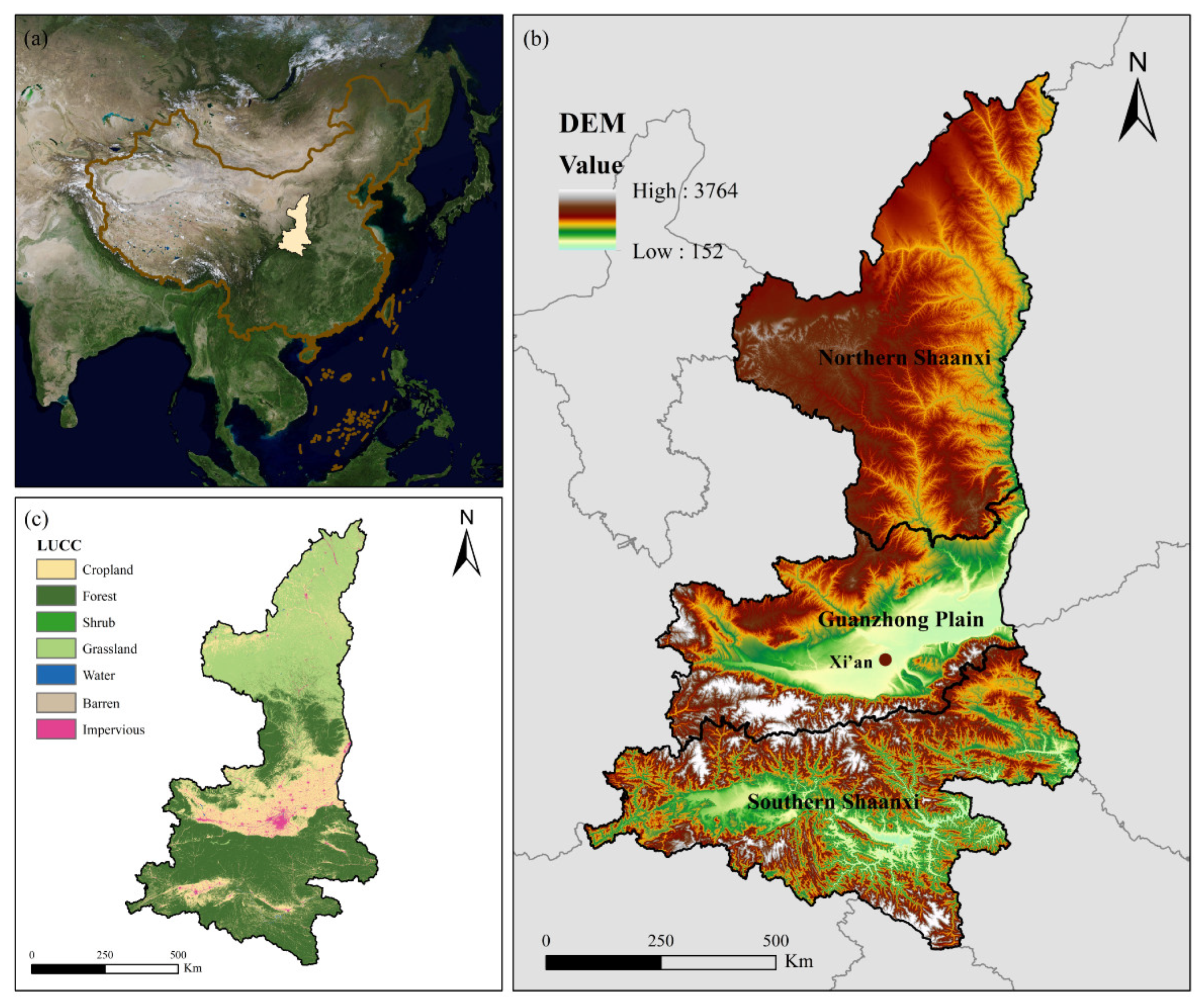
2.1. Study Area
2.2. Data Sources
2.3. Quantification of Ecosystem Services Supply and Demand
2.3.1. Supply of Ecosystem Services
- (1)
- Carbon Sequestration
- (2)
- Soil Conservation
- (3)
- Water Yield
- (4)
- Habitat quality
2.3.2. Demand of Ecosystem Services
- (1)
- Carbon Sequestration
- (2)
- Soil Conservation
- (3)
- Water Yield
- (4)
- Habitat quality
2.4. Comprehensive Urbanization Level
2.5. Calculation of Ecosystem Services Supply–Demand Ratio
2.6. Analysis of Temporal and Spatial Changes
2.7. Coupling Coordination Relationship Assessment
2.8. Random Forests
2.9. Geographically Weighted Regression (GWR) Model
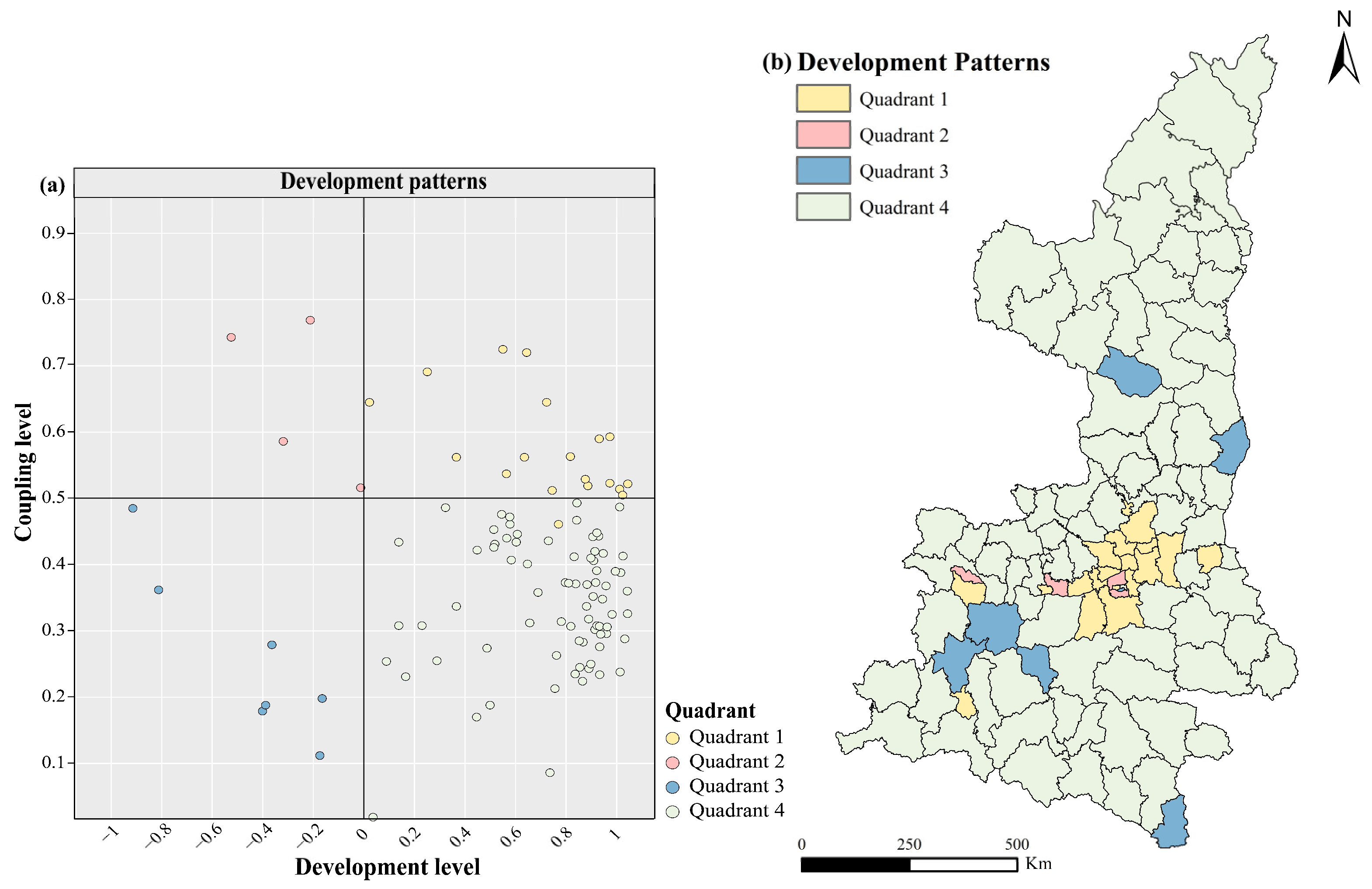
2.10. Quadrant Space Zoning
3. Results
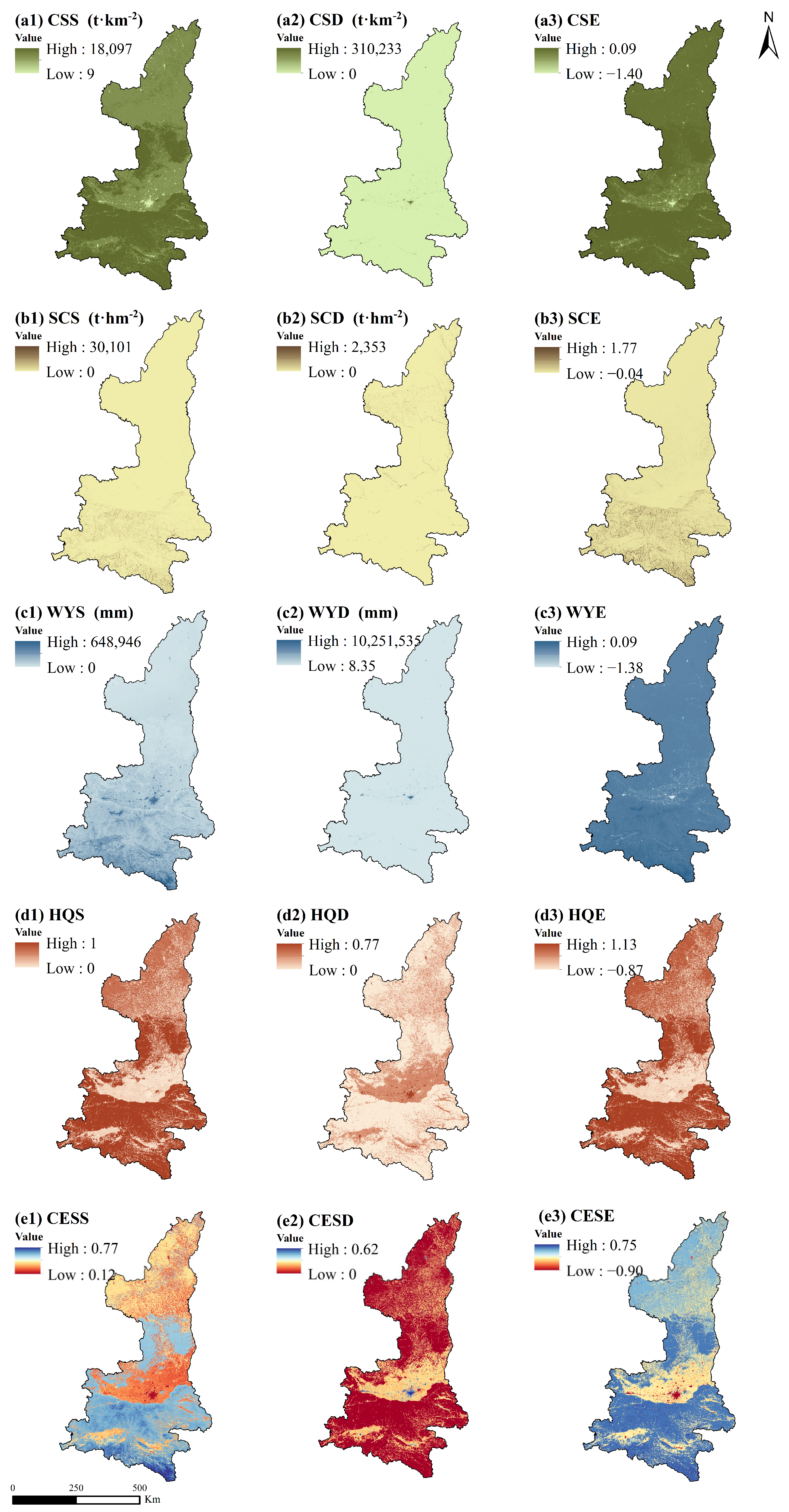
3.1. Changes in Supply and Demand for ES
3.2. Characteristics of Comprehensive Urbanization Levels
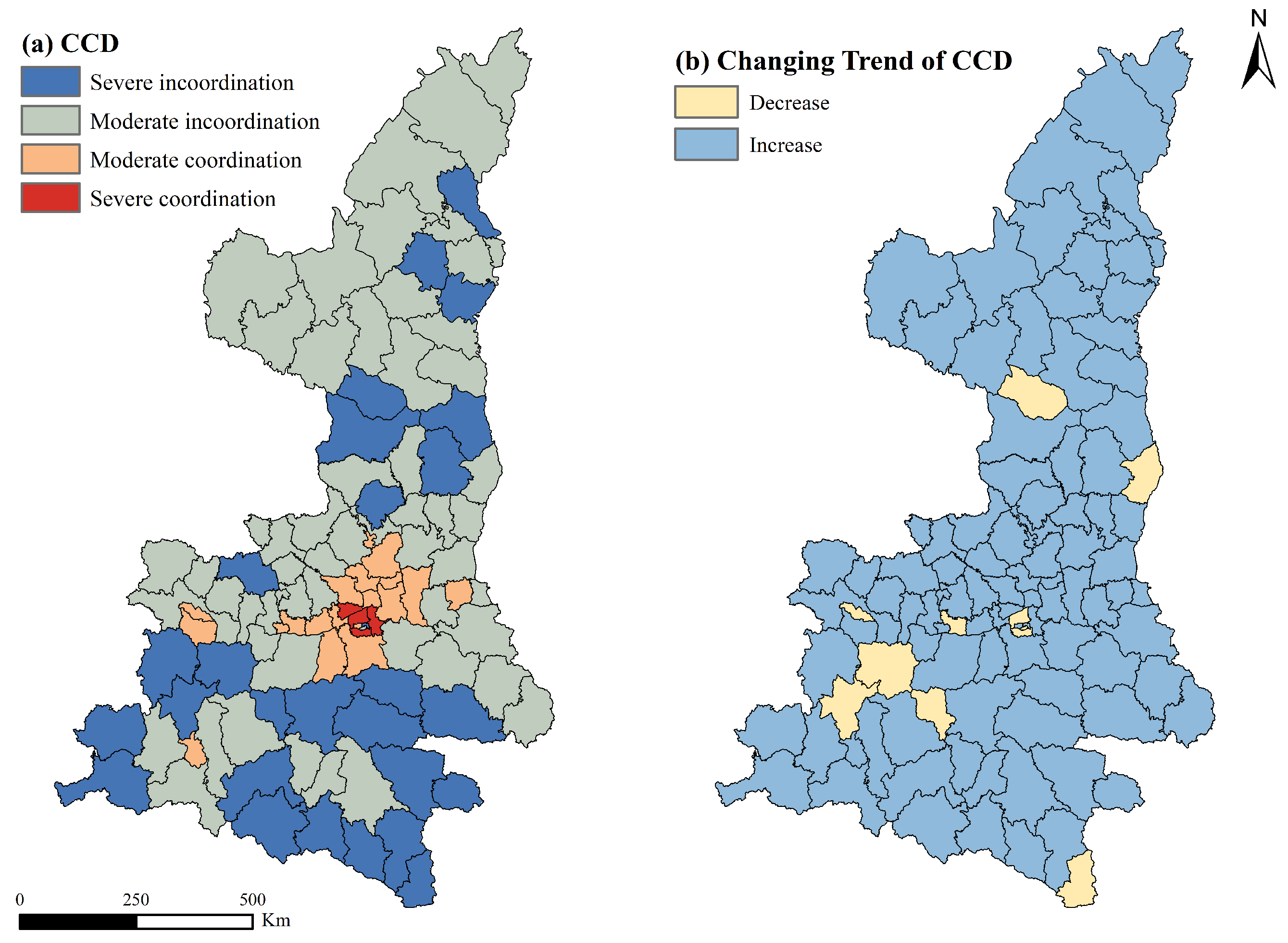
3.3. Level of Coupling Coordination and Development Trend
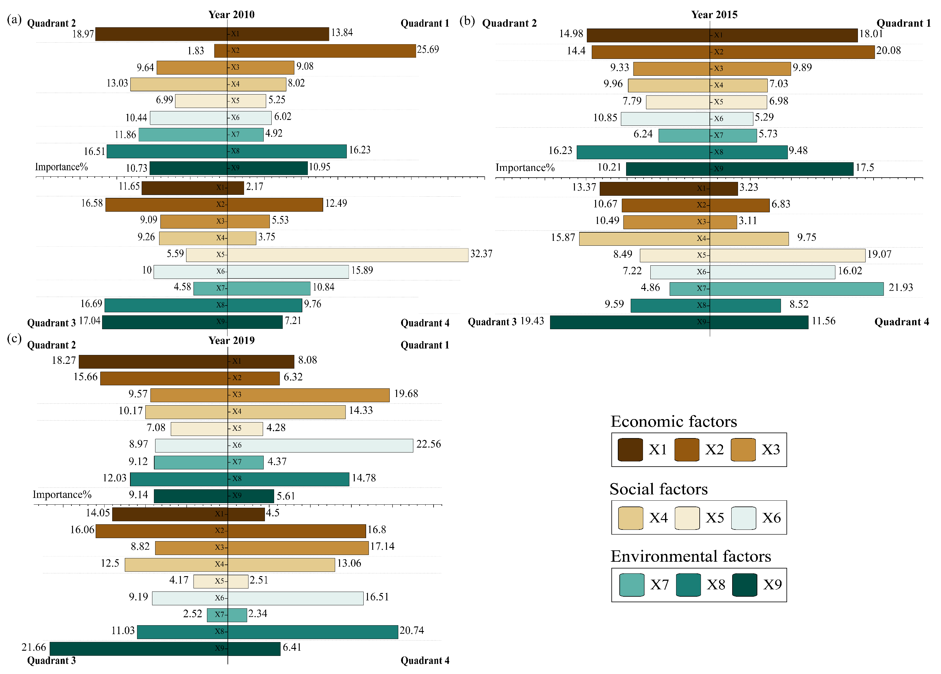
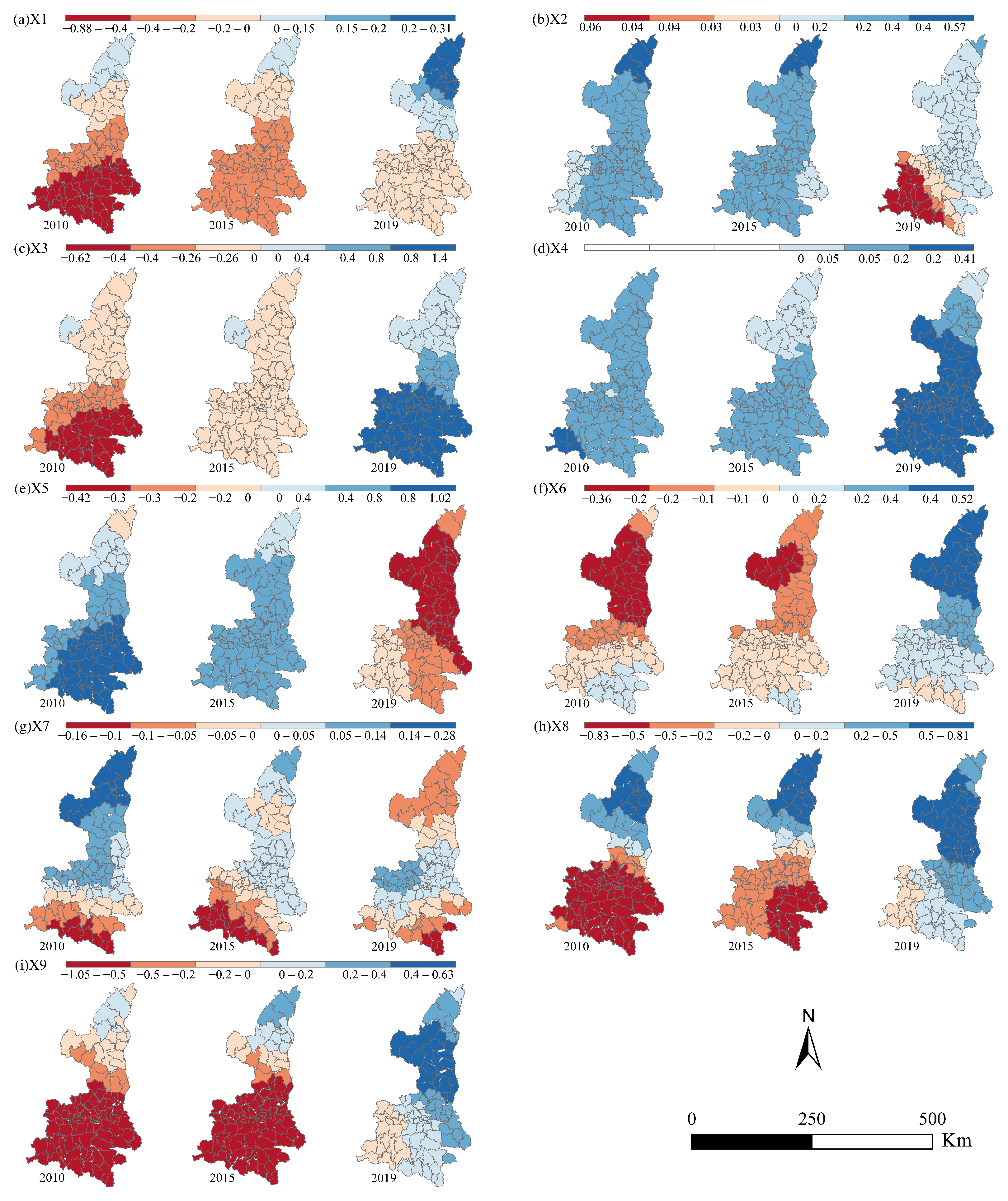
3.4. Driving Forces of the Coupling Coordination Relationship
4. Discussion
4.1. Changes in ESSDR
4.2. Driving Forces of CCD
4.3. Limitations and Prospect
5. Conclusions
Supplementary Materials
Author Contributions
Funding
Data Availability Statement
Conflicts of Interest
References
- Costanza, R.; d’Arge, R.; de Groot, R.; Farber, S.; Grasso, M.; Hannon, B.; Limburg, K.; Naeem, S.; O’Neill, R.V.; Paruelo, J.; et al. The value of the world’s ecosystem services and natural capital. Nature 1997, 387, 253–260. [Google Scholar] [CrossRef]
- Gao-Di, X.; Yu, X.; Chun-Xia, L. Institute of Geographic Sciences and Natural Resources Research, Chinese Academy of Sciences, Beijing 100101, China study on ecosystem services: Progress, limitation and basic paradigm. Chin. J. Plant Ecol. 2006, 30, 191–199. [Google Scholar] [CrossRef]
- Villamagna, A.M.; Angermeier, P.L.; Bennett, E.M. Capacity, Pressure, Demand, and Flow: A Conceptual Framework for Analyzing Ecosystem Service Provision and Delivery. Ecol. Complex. 2013, 15, 114–121. [Google Scholar] [CrossRef]
- Wei, H.; Fan, W.; Wang, X.; Lu, N.; Dong, X.; Zhao, Y.; Ya, X.; Zhao, Y. Integrating Supply and Social Demand in Ecosystem Services Assessment: A Review. Ecosyst. Serv. 2017, 25, 15–27. [Google Scholar] [CrossRef]
- Maes, J.; Crossman, N.D.; Burkhard, B. Mapping Ecosystem Services. In Routledge Handbook of Ecosystem Services; Routledge: London, UK, 2016. [Google Scholar]
- Schirpke, U.; Candiago, S.; Egarter Vigl, L.; Jäger, H.; Labadini, A.; Marsoner, T.; Meisch, C.; Tasser, E.; Tappeiner, U. Integrating Supply, Flow and Demand to Enhance the Understanding of Interactions among Multiple Ecosystem Services. Sci. Total Environ. 2019, 651, 928–941. [Google Scholar] [CrossRef]
- Li, J.; Jiang, H.; Bai, Y.; Alatalo, J.M.; Li, X.; Jiang, H.; Liu, G.; Xu, J. Indicators for Spatial–Temporal Comparisons of Ecosystem Service Status between Regions: A Case Study of the Taihu River Basin, China. Ecol. Indic. 2016, 60, 1008–1016. [Google Scholar] [CrossRef]
- Sun, X.; Tang, H.; Yang, P.; Hu, G.; Liu, Z.; Wu, J. Spatiotemporal Patterns and Drivers of Ecosystem Service Supply and Demand across the Conterminous United States: A Multiscale Analysis. Sci. Total Environ. 2020, 703, 135005. [Google Scholar] [CrossRef] [PubMed]
- Chen, D.; Li, J.; Yang, X.; Zhou, Z.; Pan, Y.; Li, M. Quantifying Water Provision Service Supply, Demand and Spatial Flow for Land Use Optimization: A Case Study in the YanHe Watershed. Ecosyst. Serv. 2020, 43, 101117. [Google Scholar] [CrossRef]
- Wei, H.; Liu, H.; Xu, Z.; Ren, J.; Lu, N.; Fan, W.; Zhang, P.; Dong, X. Linking Ecosystem Services Supply, Social Demand and Human Well-Being in a Typical Mountain–Oasis–Desert Area, Xinjiang, China. Ecosyst. Serv. 2018, 31, 44–57. [Google Scholar] [CrossRef]
- Wolff, S.; Schulp, C.J.E.; Kastner, T.; Verburg, P.H. Quantifying Spatial Variation in Ecosystem Services Demand: A Global Mapping Approach. Ecol. Econ. 2017, 136, 14–29. [Google Scholar] [CrossRef]
- Ghasemi, M.; González-García, A.; Charrahy, Z.; Serrao-Neumann, S. Utilizing Supply-Demand Bundles in Nature-Based Recreation Offers Insights into Specific Strategies for Sustainable Tourism Management. Sci. Total Environ. 2024, 922, 171185. [Google Scholar] [CrossRef] [PubMed]
- Liu, Q.; Liu, H.; Xu, G.; Lu, B.; Wang, X.; Li, J. Spatial Gradients of Supply and Demand of Ecosystem Services within Cities. Ecol. Indic. 2023, 157, 111263. [Google Scholar] [CrossRef]
- Leemans, R.; De Groot, R.S. Ecosystems and Human Well-Being: Synthesis; Millennium Ecosystem Assessment (Program), Ed.; Island Press: Washington, DC, USA, 2005; ISBN 978-1-59726-040-4. [Google Scholar]
- Arunrat, N.; Sereenonchai, S.; Wang, C. Carbon Footprint and Predicting the Impact of Climate Change on Carbon Sequestration Ecosystem Services of Organic Rice Farming and Conventional Rice Farming: A Case Study in Phichit Province, Thailand. J. Environ. Manag. 2021, 289, 112458. [Google Scholar] [CrossRef] [PubMed]
- Bai, Y.; Wong, C.P.; Jiang, B.; Hughes, A.C.; Wang, M.; Wang, Q. Developing China’s Ecological Redline Policy Using Ecosystem Services Assessments for Land Use Planning. Nat. Commun. 2018, 9, 3034. [Google Scholar] [CrossRef] [PubMed]
- Baró, F.; Palomo, I.; Zulian, G.; Vizcaino, P.; Haase, D.; Gómez-Baggethun, E. Mapping Ecosystem Service Capacity, Flow and Demand for Landscape and Urban Planning: A Case Study in the Barcelona Metropolitan Region. Land Use Policy 2016, 57, 405–417. [Google Scholar] [CrossRef]
- Huang, L.; Wang, J.; Fang, Y.; Zhai, T.; Cheng, H. An Integrated Approach towards Spatial Identification of Restored and Conserved Priority Areas of Ecological Network for Implementation Planning in Metropolitan Region. Sustain. Cities Soc. 2021, 69, 102865. [Google Scholar] [CrossRef]
- Chen, G.; Li, X.; Liu, X.; Chen, Y.; Liang, X.; Leng, J.; Xu, X.; Liao, W.; Qiu, Y.; Wu, Q.; et al. Global Projections of Future Urban Land Expansion under Shared Socioeconomic Pathways. Nat. Commun. 2020, 11, 537. [Google Scholar] [CrossRef] [PubMed]
- Liu, L.; Wu, J. Ecosystem Services-Human Wellbeing Relationships Vary with Spatial Scales and Indicators: The Case of China. Resour. Conserv. Recycl. 2021, 172, 105662. [Google Scholar] [CrossRef]
- Pan, Z.; Wang, J. Spatially Heterogeneity Response of Ecosystem Services Supply and Demand to Urbanization in China. Ecol. Eng. 2021, 169, 106303. [Google Scholar] [CrossRef]
- Zhang, Z.; Peng, J.; Xu, Z.; Wang, X.; Meersmans, J. Ecosystem Services Supply and Demand Response to Urbanization: A Case Study of the Pearl River Delta, China. Ecosyst. Serv. 2021, 49, 101274. [Google Scholar] [CrossRef]
- González-García, A.; Palomo, I.; González, J.A.; López, C.A.; Montes, C. Quantifying Spatial Supply-Demand Mismatches in Ecosystem Services Provides Insights for Land-Use Planning. Land Use Policy 2020, 94, 104493. [Google Scholar] [CrossRef]
- Shi, Y.; Shi, D.; Zhou, L.; Fang, R. Identification of Ecosystem Services Supply and Demand Areas and Simulation of Ecosystem Service Flows in Shanghai. Ecol. Indic. 2020, 115, 106418. [Google Scholar] [CrossRef]
- Cumming, G.S.; Buerkert, A.; Hoffmann, E.M.; Schlecht, E.; Von Cramon-Taubadel, S.; Tscharntke, T. Implications of Agricultural Transitions and Urbanization for Ecosystem Services. Nature 2014, 515, 50–57. [Google Scholar] [CrossRef] [PubMed]
- Peng, J.; Wang, X.; Liu, Y.; Zhao, Y.; Xu, Z.; Zhao, M.; Qiu, S.; Wu, J. Urbanization Impact on the Supply-Demand Budget of Ecosystem Services: Decoupling Analysis. Ecosyst. Serv. 2020, 44, 101139. [Google Scholar] [CrossRef]
- Yang, Z.; Hu, J.; Wang, Z.; Chen, S. A New Model Based on Coupling Coordination Analysis Incorporates the Development Rate for Urbanization and Ecosystem Services Assessment: A Case of the Yangtze River Delta. Ecol. Indic. 2024, 159, 111596. [Google Scholar] [CrossRef]
- Kadhim, N.; Ismael, N.T.; Kadhim, N.M. Urban Landscape Fragmentation as an Indicator of Urban Expansion Using Sentinel-2 Imageries. Civ. Eng. J. 2022, 8, 1799–1814. [Google Scholar] [CrossRef]
- Kumar, D.; Soni, A.; Kumar, M. Retrieval of Land Surface Temperature from Landsat-8 Thermal Infrared Sensor Data. J. Hum. Earth Future 2022, 3, 159–168. [Google Scholar] [CrossRef]
- Wei, H.; Xue, D.; Huang, J.; Liu, M.; Li, L. Identification of Coupling Relationship between Ecosystem Services and Urbanization for Supporting Ecological Management: A Case Study on Areas along the Yellow River of Henan Province. Remote Sens. 2022, 14, 2277. [Google Scholar] [CrossRef]
- Ding, T.; Chen, J.; Fang, Z.; Chen, J. Assessment of Coordinative Relationship between Comprehensive Ecosystem Service and Urbanization: A Case Study of Yangtze River Delta Urban Agglomerations, China. Ecol. Indic. 2021, 133, 108454. [Google Scholar] [CrossRef]
- Zhao, H.; Li, C.; Gao, M. Investigation of the Relationship between Supply and Demand of Ecosystem Services and the Influencing Factors in Resource-Based Cities in China. Sustainability 2023, 15, 7397. [Google Scholar] [CrossRef]
- Song, Y.; Wang, J.; Ge, Y.; Xu, C. An Optimal Parameters-Based Geographical Detector Model Enhances Geographic Characteristics of Explanatory Variables for Spatial Heterogeneity Analysis: Cases with Different Types of Spatial Data. GIScience Remote Sens. 2020, 57, 593–610. [Google Scholar] [CrossRef]
- Hou, W.; Hu, T.; Yang, L.; Liu, X.; Zheng, X.; Pan, H.; Zhang, X.; Xiao, S.; Deng, S. Matching Ecosystem Services Supply and Demand in China’s Urban Agglomerations for Multiple-Scale Management. J. Clean. Prod. 2023, 420, 138351. [Google Scholar] [CrossRef]
- Negev, M.; Sagie, H.; Orenstein, D.E.; Zemah Shamir, S.; Hassan, Y.; Amasha, H.; Raviv, O.; Fares, N.; Lotan, A.; Peled, Y.; et al. Using the Ecosystem Services Framework for Defining Diverse Human-Nature Relationships in a Multi-Ethnic Biosphere Reserve. Ecosyst. Serv. 2019, 39, 100989. [Google Scholar] [CrossRef]
- Khosravi Mashizi, A.; Sharafatmandrad, M. Investigating Tradeoffs between Supply, Use and Demand of Ecosystem Services and Their Effective Drivers for Sustainable Environmental Management. J. Environ. Manag. 2021, 289, 112534. [Google Scholar] [CrossRef] [PubMed]
- Li, J.; Xie, B.; Dong, H.; Zhou, K.; Zhang, X. The Impact of Urbanization on Ecosystem Services: Both Time and Space Are Important to Identify Driving Forces. J. Environ. Manag. 2023, 347, 119161. [Google Scholar] [CrossRef] [PubMed]
- Zhu, C.; Zhang, X.; Zhou, M.; He, S.; Gan, M.; Yang, L.; Wang, K. Impacts of Urbanization and Landscape Pattern on Habitat Quality Using OLS and GWR Models in Hangzhou, China. Ecol. Indic. 2020, 117, 106654. [Google Scholar] [CrossRef]
- Hu, J.; Zhang, J.; Li, Y. Exploring the Spatial and Temporal Driving Mechanisms of Landscape Patterns on Habitat Quality in a City Undergoing Rapid Urbanization Based on GTWR and MGWR: The Case of Nanjing, China. Ecol. Indic. 2022, 143, 109333. [Google Scholar] [CrossRef]
- Ma, S.; Wang, L.; Wang, H.; Zhang, X.; Jiang, J. Spatial Heterogeneity of Ecosystem Services in Response to Landscape Patterns under the Grain for Green Program: A Case-study in Kaihua County, China. Land Degrad. Dev. 2022, 33, 1901–1916. [Google Scholar] [CrossRef]
- Wang, L.-J.; Gong, J.-W.; Ma, S.; Wu, S.; Zhang, X.; Jiang, J. Ecosystem Service Supply–Demand and Socioecological Drivers at Different Spatial Scales in Zhejiang Province, China. Ecol. Indic. 2022, 140, 109058. [Google Scholar] [CrossRef]
- Wu, J.; Guo, X.; Zhu, Q.; Guo, J.; Han, Y.; Zhong, L.; Liu, S. Threshold Effects and Supply-Demand Ratios Should Be Considered in the Mechanisms Driving Ecosystem Services. Ecol. Indic. 2022, 142, 109281. [Google Scholar] [CrossRef]
- Chen, J.; Gao, M.; Cheng, S.; Cheng, G.S. Global 1 km × 1 km gridded revised real gross domestic product and electricity consumption during 1992–2019 based on calibrated nighttime light data. Sci Data 2022, 9, 202. [Google Scholar] [CrossRef] [PubMed]
- Bacani, V.M.; Machado Da Silva, B.H.; Ayumi De Souza Amede Sato, A.; Souza Sampaio, B.D.; Rodrigues Da Cunha, E.; Pereira Vick, E.; Ribeiro De Oliveira, V.F.; Decco, H.F. Carbon Storage and Sequestration in a Eucalyptus Productive Zone in the Brazilian Cerrado, Using the Ca-Markov/Random Forest and InVEST Models. J. Clean. Prod. 2024, 444, 141291. [Google Scholar] [CrossRef]
- Wang, Y.; Li, M.; Jin, G. Exploring the Optimization of Spatial Patterns for Carbon Sequestration Services Based on Multi-Scenario Land Use/Cover Changes in the Changchun-Jilin-Tumen Region, China. J. Clean. Prod. 2024, 438, 140788. [Google Scholar] [CrossRef]
- Phinzi, K.; Ngetar, N.S. The Assessment of Water-Borne Erosion at Catchment Level Using GIS-Based RUSLE and Remote Sensing: A Review. Int. Soil Water Conserv. Res. 2019, 7, 27–46. [Google Scholar] [CrossRef]
- Liu, M.; Dong, X.; Zhang, Y.; Wang, X.; Wei, H.; Zhang, P.; Zhang, Y. Spatiotemporal Changes in Future Water Yield and the Driving Factors under the Carbon Neutrality Target in Qinghai. Ecol. Indic. 2024, 158, 111310. [Google Scholar] [CrossRef]
- Qiu, H.; Zhang, J.; Han, H.; Cheng, X.; Kang, F. Study on the Impact of Vegetation Change on Ecosystem Services in the Loess Plateau, China. Ecol. Indic. 2023, 154, 110812. [Google Scholar] [CrossRef]
- Hillard, E.M.; Nielsen, C.K.; Groninger, J.W. Swamp Rabbits as Indicators of Wildlife Habitat Quality in Bottomland Hardwood Forest Ecosystems. Ecol. Indic. 2017, 79, 47–53. [Google Scholar] [CrossRef]
- Zhang, X.; Wan, W.; Fan, H.; Dong, X.; Lv, T. Temporal and Spatial Responses of Landscape Patterns to Habitat Quality Changes in the Poyang Lake Region, China. J. Nat. Conserv. 2024, 77, 126546. [Google Scholar] [CrossRef]
- Tian, Y.; Zhou, D.; Jiang, G. Conflict or Coordination? Multiscale Assessment of the Spatio-Temporal Coupling Relationship between Urbanization and Ecosystem Services: The Case of the Jingjinji Region, China. Ecol. Indic. 2020, 117, 106543. [Google Scholar] [CrossRef]
- Wei, W.; Nan, S.; Xie, B.; Liu, C.; Zhou, J.; Liu, C. The Spatial-Temporal Changes of Supply-Demand of Ecosystem Services and Ecological Compensation: A Case Study of Hexi Corridor, Northwest China. Ecol. Eng. 2023, 187, 106861. [Google Scholar] [CrossRef]
- Xiang, H.; Zhang, J.; Mao, D.; Wang, Z.; Qiu, Z.; Yan, H. Identifying Spatial Similarities and Mismatches between Supply and Demand of Ecosystem Services for Sustainable Northeast China. Ecol. Indic. 2022, 134, 108501. [Google Scholar] [CrossRef]
- Li, W.; Wang, Y.; Xie, S.; Cheng, X. Coupling Coordination Analysis and Spatiotemporal Heterogeneity between Urbanization and Ecosystem Health in Chongqing Municipality, China. Sci. Total Environ. 2021, 791, 148311. [Google Scholar] [CrossRef] [PubMed]
- Zhao, J.; Xiao, Y.; Sun, S.; Sang, W.; Axmacher, J.C. Does China’s Increasing Coupling of ‘Urban Population’ and ‘Urban Area’ Growth Indicators Reflect a Growing Social and Economic Sustainability? J. Environ. Manag. 2022, 301, 113932. [Google Scholar] [CrossRef] [PubMed]
- Shearman, T.M.; Varner, J.M.; Hood, S.M.; Cansler, C.A.; Hiers, J.K. Modelling Post-Fire Tree Mortality: Can Random Forest Improve Discrimination of Imbalanced Data? Ecol. Model. 2019, 414, 108855. [Google Scholar] [CrossRef]
- Xue, C.; Xue, L.; Chen, J.; Tarolli, P.; Chen, X.; Zhang, H.; Qian, J.; Zhou, Y.; Liu, X. Understanding Driving Mechanisms behind the Supply-Demand Pattern of Ecosystem Services for Land-Use Administration: Insights from a Spatially Explicit Analysis. J. Clean. Prod. 2023, 427, 139239. [Google Scholar] [CrossRef]
- Yang, M.; Gao, X.; Zhao, X.; Wu, P. Scale Effect and Spatially Explicit Drivers of Interactions between Ecosystem Services—A Case Study from the Loess Plateau. Sci. Total Environ. 2021, 785, 147389. [Google Scholar] [CrossRef]
- McMillen, D.P. Geographically Weighted Regression: The Analysis of Spatially Varying Relationships. Am. J. Agric. Econ. 2004, 86, 554–556. [Google Scholar] [CrossRef]
- Baró, F.; Gómez-Baggethun, E.; Haase, D. Ecosystem Service Bundles along the Urban-Rural Gradient: Insights for Landscape Planning and Management. Ecosyst. Serv. 2017, 24, 147–159. [Google Scholar] [CrossRef]
- Raudsepp-Hearne, C.; Peterson, G.D.; Bennett, E.M. Ecosystem Service Bundles for Analyzing Tradeoffs in Diverse Landscapes. Proc. Natl. Acad. Sci. USA 2010, 107, 5242–5247. [Google Scholar] [CrossRef]
- Bryan, B.A.; Ye, Y.; Zhang, J.; Connor, J.D. Land-Use Change Impacts on Ecosystem Services Value: Incorporating the Scarcity Effects of Supply and Demand Dynamics. Ecosyst. Serv. 2018, 32, 144–157. [Google Scholar] [CrossRef]
- Deng, C.; Liu, J.; Liu, Y.; Li, Z.; Nie, X.; Hu, X.; Wang, L.; Zhang, Y.; Zhang, G.; Zhu, D.; et al. Spatiotemporal Dislocation of Urbanization and Ecological Construction Increased the Ecosystem Service Supply and Demand Imbalance. J. Environ. Manag. 2021, 288, 112478. [Google Scholar] [CrossRef] [PubMed]
- Ren, Q.; Liu, D.; Liu, Y. Spatio-Temporal Variation of Ecosystem Services and the Response to Urbanization: Evidence Based on Shandong Province of China. Ecol. Indic. 2023, 151, 110333. [Google Scholar] [CrossRef]
- Xu, Q.; Dong, Y.; Yang, R.; Zhang, H.; Wang, C.; Du, Z. Temporal and Spatial Differences in Carbon Emissions in the Pearl River Delta Based on Multi-Resolution Emission Inventory Modeling. J. Clean. Prod. 2019, 214, 615–622. [Google Scholar] [CrossRef]
- Wan, M.; Han, Y.; Song, Y.; Hashimoto, S. Estimating and Projecting the Effects of Urbanization on the Forest Habitat Quality in a Highly Urbanized Area. Urban For. Urban Green. 2024, 94, 128270. [Google Scholar] [CrossRef]
- Han, H.; Guo, L.; Zhang, J.; Zhang, K.; Cui, N. Spatiotemporal Analysis of the Coordination of Economic Development, Resource Utilization, and Environmental Quality in the Beijing-Tianjin-Hebei Urban Agglomeration. Ecol. Indic. 2021, 127, 107724. [Google Scholar] [CrossRef]
- Zhang, X.; Liu, Y.; Wang, Y.; Yuan, X. Interactive Relationship and Zoning Management between County Urbanization and Ecosystem Services in the Loess Plateau. Ecol. Indic. 2023, 156, 111021. [Google Scholar] [CrossRef]
- Yurui, L.; Xuanchang, Z.; Zhi, C.; Zhengjia, L.; Zhi, L.; Yansui, L. Towards the Progress of Ecological Restoration and Economic Development in China’s Loess Plateau and Strategy for More Sustainable Development. Sci. Total Environ. 2021, 756, 143676. [Google Scholar] [CrossRef] [PubMed]
- Yan, J.; Liu, D.; Yao, S.; Li, J. An Empirical Study on the Impact of Industrial Structure Change on Environmental Level in China. Int. J. Econ. Energy Environ. 2023, 8, 82. [Google Scholar] [CrossRef]
- Yin, J.; Wang, S.; Gong, L. The Effects of Factor Market Distortion and Technical Innovation on China’s Electricity Consumption. J. Clean. Prod. 2018, 188, 195–202. [Google Scholar] [CrossRef]
- Bai, Y.; Liu, W.; Yang, W.; Zuo, W.; Song, H. Urbanization, Industrial Structure Upgrading, and Lottery Consumption Based on the Sustainable Development of the Emerging Markets: Evidence from China. SAGE Open 2023, 13, 21582440231182323. [Google Scholar] [CrossRef]
- Zhong, Y.; Wei, Y.D. Economic Transition, Urban Hierarchy, and Service Industry Growth in China. Tijdschr.Voor Econ. Soc. Geogr. 2018, 109, 189–209. [Google Scholar] [CrossRef]
- Henderson, J.V.; Wang, H.G. Aspects of the Rural-Urban Transformation of Countries. J. Econ. Geogr. 2005, 5, 23–42. [Google Scholar] [CrossRef]
- Shi, L. Changes of Industrial Structure and Economic Growth in Coastal Regions of China: A Threshold Panel Model Based Study. J. Coast. Res. 2020, 107, 278. [Google Scholar] [CrossRef]
- Jung, C.G.; Xu, X.; Niu, S.; Liang, J.; Chen, X.; Shi, Z.; Jiang, L.; Luo, Y. Experimental Warming Amplified Opposite Impacts of Drought vs. Wet Extremes on Ecosystem Carbon Cycle in a Tallgrass Prairie. Agric. For. Meteorol. 2019, 276–277, 107635. [Google Scholar] [CrossRef]
- Underwood, E.C.; Hollander, A.D.; Safford, H.D.; Kim, J.B.; Srivastava, L.; Drapek, R.J. The Impacts of Climate Change on Ecosystem Services in Southern California. Ecosyst. Serv. 2019, 39, 101008. [Google Scholar] [CrossRef]
- Zhang, J.; Zhang, P.; Wang, R.; Liu, Y.; Lu, S. Identifying the Coupling Coordination Relationship between Urbanization and Forest Ecological Security and Its Impact Mechanism: Case Study of the Yangtze River Economic Belt, China. J. Environ. Manag. 2023, 342, 118327. [Google Scholar] [CrossRef]


| Coupling Coordination Degree | Classification |
|---|---|
| 0 ≤ CCD ≤ 0.3 | Severe incoordination |
| 0.3 < CCD ≤ 0.5 | Moderate incoordination |
| 0.5 < CCD ≤ 0.7 | Moderate coordination |
| 0.7 < CCD ≤ 1.0 | Severe coordination |
| Year | X1 | X2 | X3 | X4 | X5 | X6 | X7 | X8 | X9 | |
|---|---|---|---|---|---|---|---|---|---|---|
| 2010 | 13.84 | 25.69 | 9.08 | 8.02 | 5.25 | 6.02 | 4.92 | 16.23 | 10.95 | |
| Quadrant 1 | 2015 | 18.01 | 20.08 | 9.89 | 7.03 | 6.98 | 5.29 | 5.73 | 9.48 | 17.5 |
| 2019 | 8.08 | 6.32 | 19.68 | 14.33 | 4.28 | 22.56 | 4.37 | 14.78 | 5.61 | |
| 2010 | 18.97 | 1.83 | 9.64 | 13.03 | 6.99 | 10.44 | 11.86 | 16.51 | 10.73 | |
| Quadrant 2 | 2015 | 14.98 | 14.4 | 9.33 | 9.96 | 7.79 | 10.85 | 6.24 | 16.23 | 10.21 |
| 2019 | 18.27 | 15.66 | 9.57 | 10.17 | 7.08 | 8.97 | 9.12 | 12.03 | 9.14 | |
| 2010 | 11.65 | 16.58 | 9.09 | 9.26 | 5.59 | 10 | 4.58 | 16.69 | 17.04 | |
| Quadrant 3 | 2015 | 13.37 | 10.67 | 10.49 | 15.87 | 8.49 | 7.22 | 4.86 | 9.59 | 19.43 |
| 2019 | 14.05 | 16.06 | 8.82 | 12.5 | 4.17 | 9.19 | 2.52 | 11.03 | 21.66 | |
| 2010 | 2.17 | 12.49 | 5.53 | 3.75 | 32.37 | 15.89 | 10.84 | 9.76 | 7.21 | |
| Quadrant 4 | 2015 | 3.23 | 6.83 | 3.11 | 9.75 | 19.07 | 16.02 | 21.93 | 8.52 | 11.56 |
| 2019 | 4.5 | 16.8 | 17.14 | 13.06 | 2.51 | 16.51 | 2.34 | 20.74 | 6.41 |
Disclaimer/Publisher’s Note: The statements, opinions and data contained in all publications are solely those of the individual author(s) and contributor(s) and not of MDPI and/or the editor(s). MDPI and/or the editor(s) disclaim responsibility for any injury to people or property resulting from any ideas, methods, instructions or products referred to in the content. |
© 2024 by the authors. Licensee MDPI, Basel, Switzerland. This article is an open access article distributed under the terms and conditions of the Creative Commons Attribution (CC BY) license (https://creativecommons.org/licenses/by/4.0/).
Share and Cite
Liu, J.; Wang, H.; Hui, L.; Tang, B.; Zhang, L.; Jiao, L. Identifying the Coupling Coordination Relationship between Urbanization and Ecosystem Services Supply–Demand and Its Driving Forces: Case Study in Shaanxi Province, China. Remote Sens. 2024, 16, 2383. https://doi.org/10.3390/rs16132383
Liu J, Wang H, Hui L, Tang B, Zhang L, Jiao L. Identifying the Coupling Coordination Relationship between Urbanization and Ecosystem Services Supply–Demand and Its Driving Forces: Case Study in Shaanxi Province, China. Remote Sensing. 2024; 16(13):2383. https://doi.org/10.3390/rs16132383
Chicago/Turabian StyleLiu, Jiamin, Hao Wang, Le Hui, Butian Tang, Liwei Zhang, and Lei Jiao. 2024. "Identifying the Coupling Coordination Relationship between Urbanization and Ecosystem Services Supply–Demand and Its Driving Forces: Case Study in Shaanxi Province, China" Remote Sensing 16, no. 13: 2383. https://doi.org/10.3390/rs16132383
APA StyleLiu, J., Wang, H., Hui, L., Tang, B., Zhang, L., & Jiao, L. (2024). Identifying the Coupling Coordination Relationship between Urbanization and Ecosystem Services Supply–Demand and Its Driving Forces: Case Study in Shaanxi Province, China. Remote Sensing, 16(13), 2383. https://doi.org/10.3390/rs16132383