


Generation of High Temporal Resolution Fractional Forest Cover Data and Its Application in Accurate Time Detection of Forest Loss
 , ,
, ,  and
and
Abstract
:1. Introduction
2. Materials and Methods
2.1. Data and Workflow
2.1.1. Vegetation Index Data
2.1.2. Relevant Fractional Forest Cover Data
2.1.3. Land Cover Data
2.1.4. Forest Cover Change Data
2.2. Long-Term Dynamic Fractional Forest Cover Mapping Based on GLASS FVC and MODIS VCF
2.2.1. Decomposition of GLASS FVC
2.2.2. Extraction of High Temporal Resolution FFC
2.3. Mapping of Long-Term Forest Loss Based on CCDC
2.4. Performance Validation Methods
2.4.1. Validation of GLASS FFC Product
2.4.2. Validation of the Forest Loss Identification
3. Results
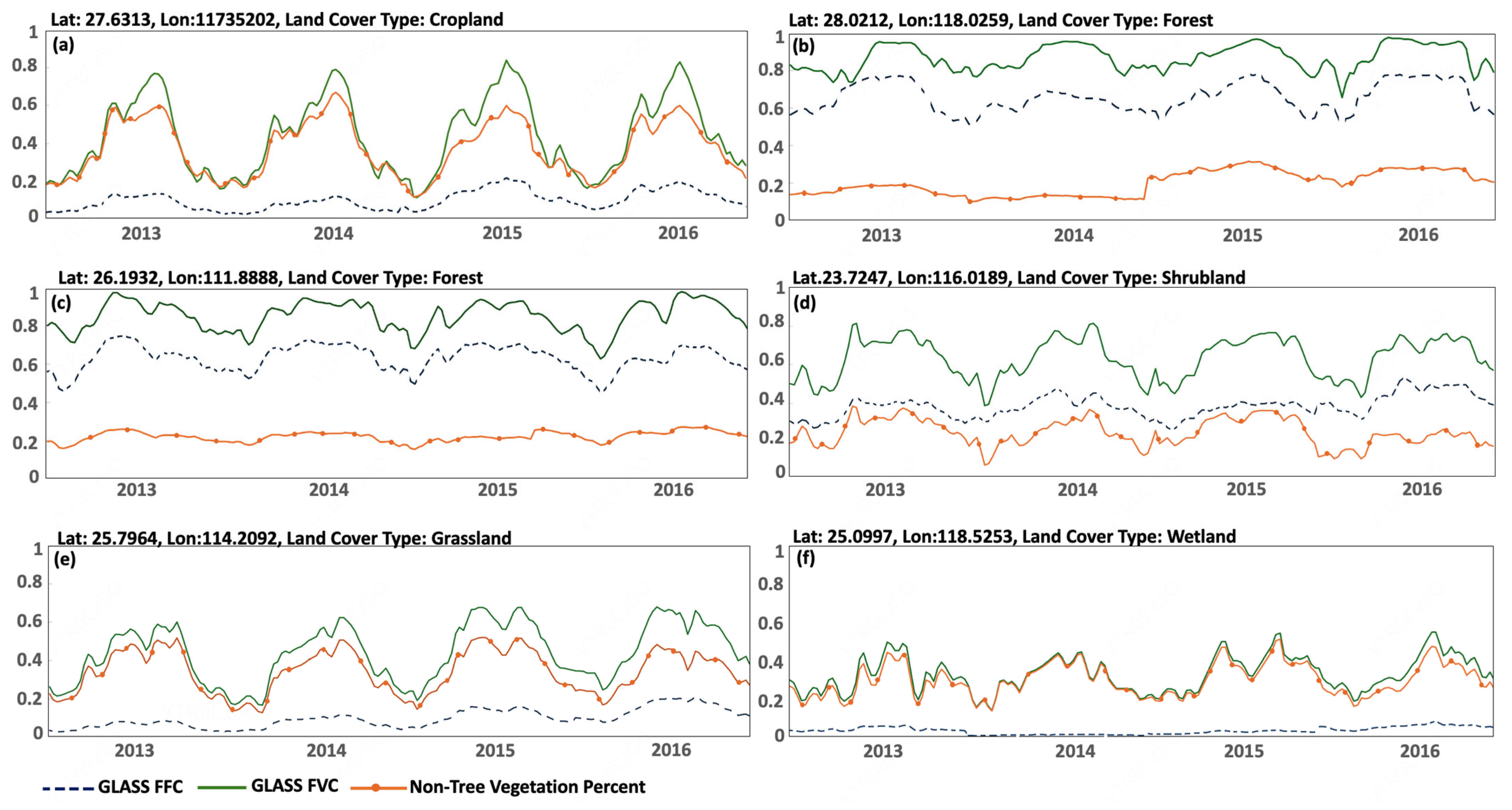
3.1. Spatial Patterns and Time Series of GLASS FFC
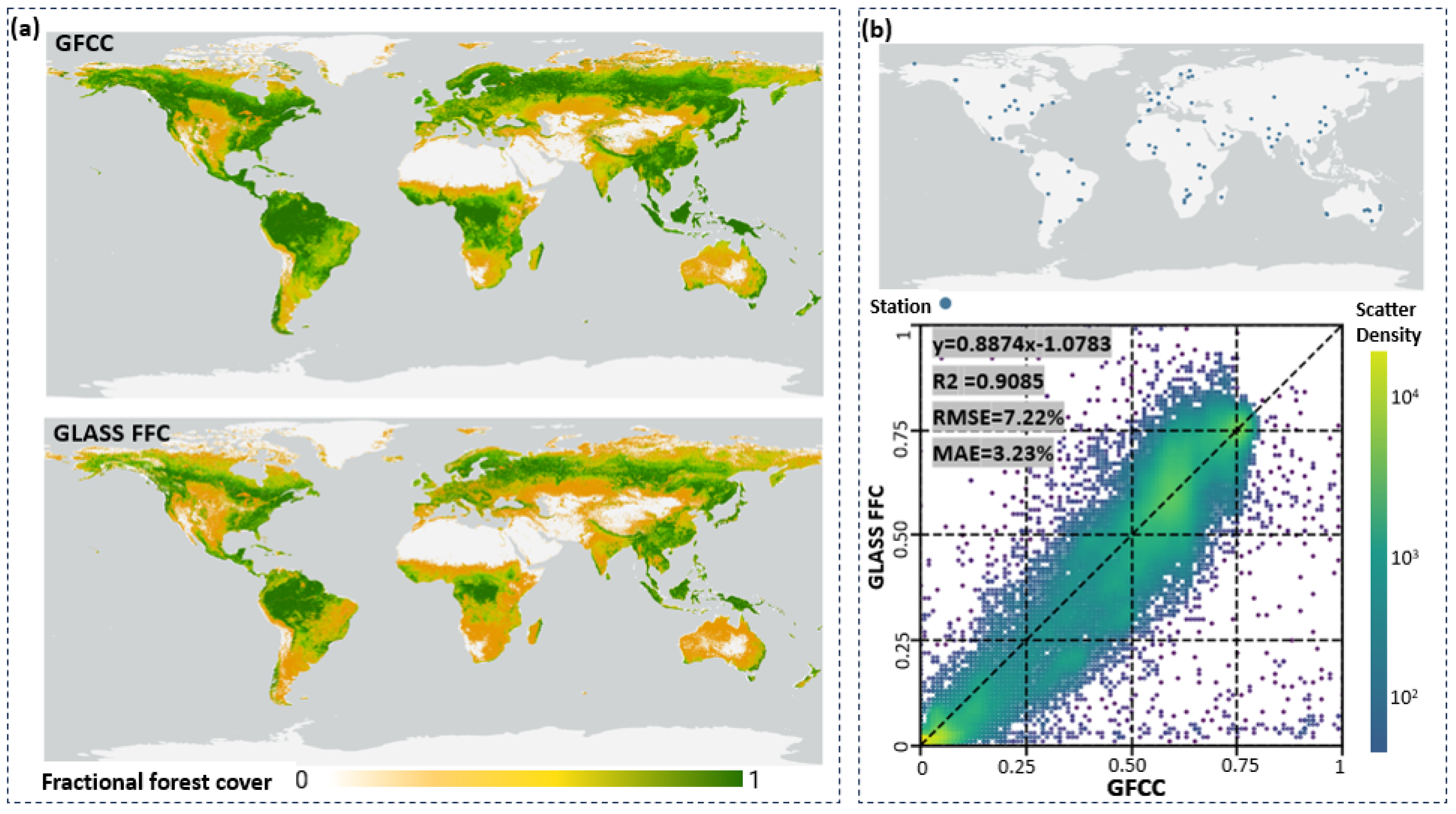
3.2. Accuracy Evaluation and Product Comparison of GLASS FFC
3.3. Forest Loss Identification Based on GLASS FFC and CCDC
3.3.1. Post-Processing of the CCDC
3.3.2. Accuracy Assessment of Forest Loss Detection Results
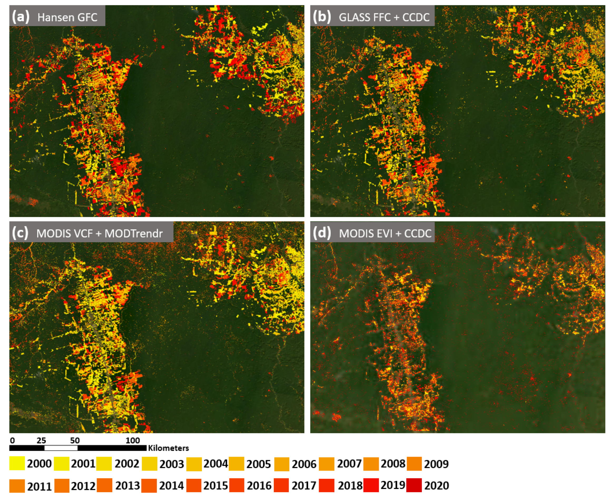
3.3.3. Comparison with Other Vegetation Datasets
4. Discussion
4.1. Characteristics of GLASS FFC Data
4.2. Application Potential and Prospects
4.3. Limitations and Future Work
5. Conclusions
Author Contributions
Funding
Data Availability Statement
Acknowledgments
Conflicts of Interest
References
- Palmer, L. How Trees and Forests Reduce Risks from Climate Change. Nat. Clim. Chang. 2021, 11, 374–377. [Google Scholar] [CrossRef]
- Anderegg, W.R.L.; Trugman, A.T.; Badgley, G.; Anderson, C.M.; Bartuska, A.; Ciais, P.; Cullenward, D.; Field, C.B.; Freeman, J.; Goetz, S.J.; et al. Climate-Driven Risks to the Climate Mitigation Potential of Forests. Science 2020, 368, eaaz7005. [Google Scholar] [CrossRef] [PubMed]
- Cook-Patton, S.C.; Leavitt, S.M.; Gibbs, D.; Harris, N.L.; Lister, K.; Anderson-Teixeira, K.J.; Briggs, R.D.; Chazdon, R.L.; Crowther, T.W.; Ellis, P.W.; et al. Mapping Carbon Accumulation Potential from Global Natural Forest Regrowth. Nature 2020, 585, 545–550. [Google Scholar] [CrossRef] [PubMed]
- Sommerfeld, A.; Senf, C.; Buma, B.; D’Amato, A.W.; Després, T.; Díaz-Hormazábal, I.; Fraver, S.; Frelich, L.E.; Gutiérrez, Á.G.; Hart, S.J.; et al. Patterns and Drivers of Recent Disturbances across the Temperate Forest Biome. Nat. Commun. 2018, 9, 4355. [Google Scholar] [CrossRef] [PubMed]
- Li, Y.; Wu, Z.; Xu, X.; Fan, H.; Tong, X.; Liu, J. Forest Disturbances and the Attribution Derived from Yearly Landsat Time Series over 1990–2020 in the Hengduan Mountains Region of Southwest China. For. Ecosyst. 2021, 8, 73. [Google Scholar] [CrossRef]
- Hansen, M.C.; DeFries, R.S.; Townshend, J.R.G.; Carroll, M.; Dimiceli, C.; Sohlberg, R.A. Global Percent Tree Cover at a Spatial Resolution of 500 Meters: First Results of the MODIS Vegetation Continuous Fields Algorithm. Earth Interact. 2003, 7, 1–15. [Google Scholar] [CrossRef]
- Jia, K.; Liang, S.; Wei, X.; Li, Q.; Du, X.; Jiang, B.; Yao, Y.; Zhao, X.; Li, Y. Fractional Forest Cover Changes in Northeast China from 1982 to 2011 and Its Relationship with Climatic Variations. IEEE J. Sel. Top. Appl. Earth Obs. Remote Sens. 2015, 8, 775–783. [Google Scholar] [CrossRef]
- Liu, X.; Liang, S.; Li, B.; Ma, H.; He, T. Mapping 30 m Fractional Forest Cover over China’s Three-North Region from Landsat-8 Data Using Ensemble Machine Learning Methods. Remote Sens. 2021, 13, 2592. [Google Scholar] [CrossRef]
- Pradhan, P.; Costa, L.; Rybski, D.; Lucht, W.; Kropp, J.P. A Systematic Study of Sustainable Development Goal (SDG) Interactions. Earth’s Future 2017, 5, 1169–1179. [Google Scholar] [CrossRef]
- DiMiceli, C.; Townshend, J.; Carroll, M.; Sohlberg, R. Evolution of the Representation of Global Vegetation by Vegetation Continuous Fields. Remote Sens. Environ. 2021, 254, 112271. [Google Scholar] [CrossRef]
- Hansen, M.; DiMiceli, C.; Sohlberg, R. User Guide for the MEaSURES Vegetation Continuous Fields Product, Version 1; University of Maryland: College Park, MD, USA, 2017. [Google Scholar]
- Sexton, J.O.; Song, X.-P.; Feng, M.; Noojipady, P.; Anand, A.; Huang, C.; Kim, D.-H.; Collins, K.M.; Channan, S.; DiMiceli, C.; et al. Global, 30-m Resolution Continuous Fields of Tree Cover: Landsat-Based Rescaling of MODIS Vegetation Continuous Fields with Lidar-Based Estimates of Error. Int. J. Digit. Earth 2013, 6, 427–448. [Google Scholar] [CrossRef]
- Shimada, M.; Isoguchi, O.; Motooka, T.; Shiraishi, T.; Mukaida, A.; Okumura, H.; Otaki, T.; Itoh, T. Generation of 10 m Resolution PALSAR and JERS-SAR Mosaic and Forest/Non-Forest Maps for Forest Carbon Tracking. In Proceedings of the 2011 IEEE International Geoscience and Remote Sensing Symposium, Vancouver, BC, Canada, 24–29 July 2011; Available online: https://ieeexplore.ieee.org/abstract/document/6049978 (accessed on 21 April 2024).
- Hansen, M.C.; Potapov, P.V.; Moore, R.; Hancher, M.; Turubanova, S.A.; Tyukavina, A.; Thau, D.; Stehman, S.V.; Goetz, S.J.; Loveland, T.R.; et al. High-Resolution Global Maps of 21st-Century Forest Cover Change. Science 2013, 342, 850–853. [Google Scholar] [CrossRef] [PubMed]
- Hansen, M.C.; Egorov, A.; Roy, D.P.; Potapov, P.; Ju, J.; Turubanova, S.; Kommareddy, I.; Loveland, T.R. Continuous Fields of Land Cover for the Conterminous United States Using Landsat Data: First Results from the Web-Enabled Landsat Data (WELD) Project. Remote Sens. Lett. 2011, 2, 279–288. [Google Scholar] [CrossRef]
- Liu, X.; Liang, S.; Ma, H.; Li, B.; Zhang, Y.; Li, Y.; He, T.; Zhang, G.; Xu, J.; Xiong, C.; et al. Landsat-Observed Changes in Forest Cover and Attribution Analysis over Northern China from 1996–2020. GIScience Remote Sens. 2024, 61, 2300214. [Google Scholar] [CrossRef]
- Yan, Y.; Piao, S.; Hammond, W.M.; Chen, A.; Hong, S.; Xu, H.; Munson, S.M.; Myneni, R.B.; Allen, C.D. Climate-Induced Tree-Mortality Pulses Are Obscured by Broad-Scale and Long-Term Greening. Nat. Ecol. Evol. 2024, 8, 912–923. [Google Scholar] [CrossRef]
- Shimizu, K.; Ota, T.; Mizoue, N. Accuracy Assessments of Local and Global Forest Change Data to Estimate Annual Disturbances in Temperate Forests. Remote Sens. 2020, 12, 2438. [Google Scholar] [CrossRef]
- Galiatsatos, N.; Donoghue, D.N.; Watt, P.; Bholanath, P.; Pickering, J.; Hansen, M.C.; Mahmood, A.R. An Assessment of Global Forest Change Datasets for National Forest Monitoring and Reporting. Remote Sens. 2020, 12, 1790. [Google Scholar] [CrossRef]
- Frantz, D.; Röder, A.; Udelhoven, T.; Schmidt, M. Forest Disturbance Mapping Using Dense Synthetic Landsat/MODIS Time-Series and Permutation-Based Disturbance Index Detection. Remote Sens. 2016, 8, 277. [Google Scholar] [CrossRef]
- Tang, X.; Bullock, E.L.; Olofsson, P.; Woodcock, C.E. Can VIIRS Continue the Legacy of MODIS for near Real-Time Monitoring of Tropical Forest Disturbance? Remote Sens. Environ. 2020, 249, 112024. [Google Scholar] [CrossRef]
- Tang, X.; Bullock, E.L.; Olofsson, P.; Estel, S.; Woodcock, C.E. Near Real-Time Monitoring of Tropical Forest Disturbance: New Algorithms and Assessment Framework. Remote Sens. Environ. 2019, 224, 202–218. [Google Scholar] [CrossRef]
- Ferrara, C.; Marchi, M.; Fabbio, G.; Fares, S.; Bertini, G.; Piovosi, M.; Salvati, L. Exploring Nonlinear Intra-Annual Growth Dynamics in Fagus sylvatica L. Trees at the Italian ICP-Forests Level II Network. Forests 2019, 10, 584. [Google Scholar] [CrossRef]
- Martínez-Sancho, E.; Gutiérrez, E.; Valeriano, C.; Ribas, M.; Popkova, M.I.; Shishov, V.V.; Dorado-Liñán, I. Intra- and Inter-Annual Growth Patterns of a Mixed Pine-Oak Forest under Mediterranean Climate. Forests 2021, 12, 1746. [Google Scholar] [CrossRef]
- Stanimirova, R.; Tarrio, K.; Turlej, K.; McAvoy, K.; Stonebrook, S.; Hu, K.-T.; Arévalo, P.; Bullock, E.L.; Zhang, Y.; Woodcock, C.E.; et al. A Global Land Cover Training Dataset from 1984 to 2020. Sci. Data 2023, 10, 879. [Google Scholar] [CrossRef] [PubMed]
- Halperin, J.; LeMay, V.; Coops, N.; Verchot, L.; Marshall, P.; Lochhead, K. Canopy cover estimation in miombo woodlands of Zambia: Comparison of Landsat 8 OLI versus RapidEye imagery using parametric, nonparametric, and semiparametric methods. Remote. Sens. Environ. 2016, 179, 170–182. [Google Scholar] [CrossRef]
- Jia, T.; Li, Y.; Shi, W.; Zhu, L. Deriving a Forest Cover Map in Kyrgyzstan Using a Hybrid Fusion Strategy. Remote. Sens. 2019, 11, 2325. [Google Scholar] [CrossRef]
- De Jong, R.; de Bruin, S.; de Wit, A.; Schaepman, M.E.; Dent, D.L. Analysis of Monotonic Greening and Browning Trends from Global NDVI Time-Series. Remote Sens. Environ. 2011, 115, 692–702. [Google Scholar] [CrossRef]
- Kokubu, Y.; Hara, S.; Tani, A. Mapping Seasonal Tree Canopy Cover and Leaf Area Using Worldview-2/3 Satellite Imagery: A Megacity-Scale Case Study in Tokyo Urban Area. Remote Sens. 2020, 12, 1505. [Google Scholar] [CrossRef]
- Tucker, C.J. Red and Photographic Infrared Linear Combinations for Monitoring Vegetation. Remote Sens. Environ. 1979, 8, 127–150. [Google Scholar] [CrossRef]
- Liu, L.; Zhang, X.; Gao, Y.; Chen, X.; Shuai, X.; Mi, J. Finer-Resolution Mapping of Global Land Cover: Recent Developments, Consistency Analysis, and Prospects. J. Remote Sens. 2021, 2021, 5289697. [Google Scholar] [CrossRef]
- Yang, L.; Jia, K.; Liang, S.; Liu, J.; Wang, X. Comparison of Four Machine Learning Methods for Generating the GLASS Fractional Vegetation Cover Product from MODIS Data. Remote Sens. 2016, 8, 682. [Google Scholar] [CrossRef]
- Jia, K.; Liang, S.; Liu, S.; Li, Y.; Xiao, Z.; Yao, Y.; Jiang, B.; Zhao, X.; Wang, X.; Xu, S.; et al. Global Land Surface Fractional Vegetation Cover Estimation Using General Regression Neural Networks from MODIS Surface Reflectance. IEEE Trans. Geosci. Remote Sens. 2015, 53, 4787–4796. [Google Scholar] [CrossRef]
- North, P.R. Estimation of fAPAR, LAI, and Vegetation Fractional Cover from ATSR-2 Imagery. Remote Sens. Environ. 2002, 80, 114–121. [Google Scholar] [CrossRef]
- Jia, K.; Yang, L.; Liang, S.; Xiao, Z.; Zhao, X.; Yao, Y.; Zhang, X.; Jiang, B.; Liu, D. Long-Term Global Land Surface Satellite (GLASS) Fractional Vegetation Cover Product Derived from MODIS and AVHRR Data. IEEE J. Sel. Top. Appl. Earth Obs. Remote Sens. 2018, 12, 508–518. [Google Scholar] [CrossRef]
- Jia, K.; Liang, S.; Wei, X.; Yao, Y.; Yang, L.; Zhang, X.; Liu, D. Validation of Global LAnd Surface Satellite (GLASS) Fractional Vegetation Cover Product from MODIS Data in an Agricultural Region. Remote Sens. Lett. 2018, 9, 847–856. [Google Scholar] [CrossRef]
- Xiong, C.; Ma, H.; Liang, S.; He, T.; Zhang, Y.; Zhang, G.; Xu, J. Improved Global 250 m 8-Day NDVI and EVI Products from 2000–2021 Using the LSTM Model. Sci. Data 2023, 10, 800. [Google Scholar] [CrossRef]
- Song, X.-P.; Huang, C.; Sexton, J.O.; Channan, S.; Townshend, J.R. Annual Detection of Forest Cover Loss Using Time Series Satellite Measurements of Percent Tree Cover. Remote Sens. 2014, 6, 8878–8903. [Google Scholar] [CrossRef]
- Tang, H.; Armston, J.; Dubayah, R. Algorithm Theoretical Basis Document (ATBD) for GEDI L2B Footprint Canopy Cover and Vertical Profile Metrics; Goddard Space Flight Center: Greenbelt, MD, USA, 2019. [Google Scholar]
- Hoffrén, R.; Lamelas, M.T.; de la Riva, J.; Domingo, D.; Montealegre, A.L.; García-Martín, A.; Revilla, S. Assessing GEDI-NASA System for Forest Fuels Classification Using Machine Learning Techniques. Int. J. Appl. Earth Obs. Geoinf. 2023, 116, 103175. [Google Scholar] [CrossRef]
- Tang, H.; Song, X.-P.; Zhao, F.A.; Strahler, A.H.; Schaaf, C.L.; Goetz, S.; Huang, C.; Hansen, M.C.; Dubayah, R. Definition and Measurement of Tree Cover: A Comparative Analysis of Field-, Lidar-and Landsat-Based Tree Cover Estimations in the Sierra National Forests, USA. Agric. For. Meteorol. 2019, 268, 258–268. [Google Scholar] [CrossRef]
- Fayad, I.; Baghdadi, N.; Lahssini, K. An Assessment of the GEDI Lasers’ Capabilities in Detecting Canopy Tops and Their Penetration in a Densely Vegetated, Tropical Area. Remote Sens. 2022, 14, 2969. [Google Scholar] [CrossRef]
- Adam, M.; Urbazaev, M.; Dubois, C.; Schmullius, C. Accuracy Assessment of GEDI Terrain Elevation and Canopy Height Estimates in European Temperate Forests: Influence of Environmental and Acquisition Parameters. Remote Sens. 2020, 12, 3948. [Google Scholar] [CrossRef]
- Marselis, S.M.; Keil, P.; Chase, J.M.; Dubayah, R. The Use of GEDI Canopy Structure for Explaining Variation in Tree Species Richness in Natural Forests. Environ. Res. Lett. 2022, 17, 045003. [Google Scholar] [CrossRef]
- Tang, H.; Armston, J.; Hancock, S.; Marselis, S.; Goetz, S.; Dubayah, R. Characterizing Global Forest Canopy Cover Distribution Using Spaceborne Lidar. Remote Sens. Environ. 2019, 231, 111262. [Google Scholar] [CrossRef]
- Chen, J.; Chen, J.; Liao, A.; Cao, X.; Chen, L.; Chen, X.; He, C.; Han, G.; Peng, S.; Lu, M.; et al. Global Land Cover Mapping at 30 m Resolution: A POK-Based Operational Approach. ISPRS J. Photogramm. Remote Sens. 2015, 103, 7–27. [Google Scholar] [CrossRef]
- McDowell, N.G.; Allen, C.D.; Anderson-Teixeira, K.; Aukema, B.H.; Bond-Lamberty, B.; Chini, L.; Clark, J.S.; Dietze, M.; Grossiord, C.; Hanbury-Brown, A.; et al. Pervasive Shifts in Forest Dynamics in a Changing World. Science 2020, 368, eaaz9463. [Google Scholar] [CrossRef] [PubMed]
- Bastin, J.-F.; Finegold, Y.; Garcia, C.; Mollicone, D.; Rezende, M.; Routh, D.; Zohner, C.M.; Crowther, T.W. The Global Tree Restoration Potential. Science 2019, 365, 76–79. [Google Scholar] [CrossRef] [PubMed]
- Feng, Y.; Ziegler, A.D.; Elsen, P.R.; Liu, Y.; He, X.; Spracklen, D.V.; Holden, J.; Jiang, X.; Zheng, C.; Zeng, Z. Upward Expansion and Acceleration of Forest Clearance in the Mountains of Southeast Asia. Nat. Sustain. 2021, 4, 892–899. [Google Scholar] [CrossRef]
- Wang, H.; Cai, L.; Wen, X.; Fan, D.; Wang, Y. Land Cover Change and Multiple Remotely Sensed Datasets Consistency in China. Ecosyst. Health Sustain. 2022, 8, 2040385. [Google Scholar] [CrossRef]
- Andreacci, F.; Marenzi, R.C. Accounting for Twenty-First-Century Annual Forest Loss in the Atlantic Forest of Brazil Using High-Resolution Global Maps. Int. J. Remote Sens. 2020, 41, 4408–4420. [Google Scholar] [CrossRef]
- Cunningham, D.; Cunningham, P.; Fagan, M.E. Identifying Biases in Global Tree Cover Products: A Case Study in Costa Rica. Forests 2019, 10, 853. [Google Scholar] [CrossRef]
- Zhu, Z.; Woodcock, C.E. Continuous Change Detection and Classification of Land Cover Using All Available Landsat Data. Remote Sens. Environ. 2014, 144, 152–171. [Google Scholar] [CrossRef]
- Pasquarella, V.J.; Arévalo, P.; Bratley, K.H.; Bullock, E.L.; Gorelick, N.; Yang, Z.; Kennedy, R.E. Demystifying LandTrendr and CCDC Temporal Segmentation. Int. J. Appl. Earth Obs. Geoinf. 2022, 110, 102806. [Google Scholar] [CrossRef]
- Chen, S.; Woodcock, C.E.; Bullock, E.L.; Arévalo, P.; Torchinava, P.; Peng, S.; Olofsson, P. Monitoring Temperate Forest Degradation on Google Earth Engine Using Landsat Time Series Analysis. Remote Sens. Environ. 2021, 265, 112648. [Google Scholar] [CrossRef]
- Shimizu, K.; Ota, T.; Mizoue, N.; Yoshida, S. A Comprehensive Evaluation of Disturbance Agent Classification Approaches: Strengths of Ensemble Classification, Multiple Indices, Spatio-Temporal Variables, and Direct Prediction. ISPRS J. Photogramm. Remote Sens. 2019, 158, 99–112. [Google Scholar] [CrossRef]
- Arévalo, P.; Bullock, E.L.; Woodcock, C.E.; Olofsson, P. A Suite of Tools for Continuous Land Change Monitoring in Google Earth Engine. Front. Clim. 2020, 2, 576740. [Google Scholar] [CrossRef]
- Shimabukuro, Y.E.; Santos, J.; Formaggio, A.; Duarte, V.; Rudorff, B.; Achard, F.; Hansen, M. The Brazilian Amazon monitoring program: PRODES and DETER projects. Glob. For. Monit. Earth Obs. 2016, 2012, 153–169. [Google Scholar]
- Garrigues, S.; Lacaze, R.; Baret, F.J.T.M.; Morisette, J.T.; Weiss, M.; Nickeson, J.E.; Fernandeset, R. Validation and intercomparison of global Leaf Area Index products derived from remote sensing data. J. Geophys. Res. Biogeosci. 2008, 113, G2. [Google Scholar] [CrossRef]
- Sulla-Menashe, D.; Kennedy, R.E.; Yang, Z.; Braaten, J.; Krankina, O.N.; Friedl, M.A. Detecting Forest Disturbance in the Pacific Northwest from MODIS Time Series Using Temporal Segmentation. Remote Sens. Environ. 2014, 151, 114–123. [Google Scholar] [CrossRef]
- Li, M.; Huang, C.; Zhu, Z.; Shi, H.; Lu, H.; Peng, S. Assessing Rates of Forest Change and Fragmentation in Alabama, USA, Using the Vegetation Change Tracker Model. For. Ecol. Manag. 2009, 257, 1480–1488. [Google Scholar] [CrossRef]
- Rahman, A.F.; Sims, D.A.; Cordova, V.D.; El-Masri, B.Z. Potential of MODIS EVI and Surface Temperature for Directly Estimating Per-Pixel Ecosystem C Fluxes. Geophys. Res. Lett. 2005, 32, L19404. [Google Scholar] [CrossRef]
- Marshall, A.R.; Waite, C.E.; Pfeifer, M.; Banin, L.F.; Rakotonarivo, S.; Chomba, S.; Herbohn, J.; Gilmour, D.A.; Brown, M.; Chazdon, R.L. Fifteen Essential Science Advances Needed for Effective Restoration of the World’s Forest Landscapes. Philos. Trans. R. Soc. Lond. B Biol. Sci. 2022, 378, 20210065. [Google Scholar] [CrossRef]
- Liu, Y.; Ziegler, A.D.; Wu, J.; Liang, S.; Wang, D.; Xu, R.; Duangnamon, D.; Li, H.; Zeng, Z. Effectiveness of Protected Areas in Preventing Forest Loss in a Tropical Mountain Region. Ecol. Indic. 2022, 136, 108697. [Google Scholar] [CrossRef]
- Altman, J.; Fibich, P.; Trotsiuk, V.; Altmanova, N. Global Pattern of Forest Disturbances and Its Shift under Climate Change. Sci. Total Environ. 2024, 915, 170117. [Google Scholar] [CrossRef] [PubMed]
- Pickering, J.; Stehman, S.V.; Tyukavina, A.; Potapov, P.; Watt, P.; Jantz, S.M.; Bholanath, P.; Hansen, M.C. Quantifying the Trade-off between Cost and Precision in Estimating Area of Forest Loss and Degradation Using Probability Sampling in Guyana. Remote Sens. Environ. 2019, 221, 122–135. [Google Scholar] [CrossRef]
- Yuan, Y.; Lin, L. Self-Supervised Pretraining of Transformers for Satellite Image Time Series Classification. IEEE J. Sel. Top. Appl. Earth Obs. Remote Sens. 2021, 14, 474–487. [Google Scholar] [CrossRef]
- Yuan, Y.; Lin, L.; Huo, L.-Z.; Kong, Y.-L.; Zhou, Z.-G.; Wu, B.; Jia, Y. Using An Attention-Based LSTM Encoder–Decoder Network for Near Real-Time Disturbance Detection. IEEE J. Sel. Top. Appl. Earth Obs. Remote Sens. 2020, 13, 1819–1832. [Google Scholar] [CrossRef]
- Hasan, M.E.; Nath, B.; Sarker, A.H.M.R.; Wang, Z.; Zhang, L.; Yang, X.; Nobi, M.N.; Røskaft, E.; Chivers, D.J.; Suza, M. Applying Multi-Temporal Landsat Satellite Data and Markov-Cellular Automata to Predict Forest Cover Change and Forest Degradation of Sundarban Reserve Forest, Bangladesh. Forests 2020, 11, 1016. [Google Scholar] [CrossRef]
- Vieilledent, G.; Grinand, C.; Rakotomalala, F.A.; Ranaivosoa, R.; Rakotoarijaona, J.-R.; Allnutt, T.F.; Achard, F. Combining Global Tree Cover Loss Data with Historical National Forest Cover Maps to Look at Six Decades of Deforestation and Forest Fragmentation in Madagascar. Biol. Conserv. 2018, 222, 189–197. [Google Scholar] [CrossRef]
- Aziz, G.; Minallah, N.; Saeed, A.; Frnda, J.; Khan, W. Remote Sensing Based Forest Cover Classification Using Machine Learning. Sci. Rep. 2024, 14, 69. [Google Scholar] [CrossRef] [PubMed]
- Tariq, A.; Jiango, Y.; Li, Q.; Gao, J.; Lu, L.; Soufan, W.; Almutairi, K.F.; Habib-ur-Rahman, M. Modelling, Mapping and Monitoring of Forest Cover Changes, Using Support Vector Machine, Kernel Logistic Regression and Naive Bayes Tree Models with Optical Remote Sensing Data. Heliyon 2023, 9, e13212. [Google Scholar] [CrossRef]
- Kennedy, R.E.; Yang, Z.; Cohen, W.B.; Pfaff, E.; Braaten, J.; Nelson, P. Spatial and Temporal Patterns of Forest Disturbance and Regrowth within the Area of the Northwest Forest Plan. Remote Sens. Environ. 2012, 122, 117–133. [Google Scholar] [CrossRef]


| Study Area | Sample Size | Step Size | Optimal Threshold | Overall Accuracy at Optimal Threshold |
|---|---|---|---|---|
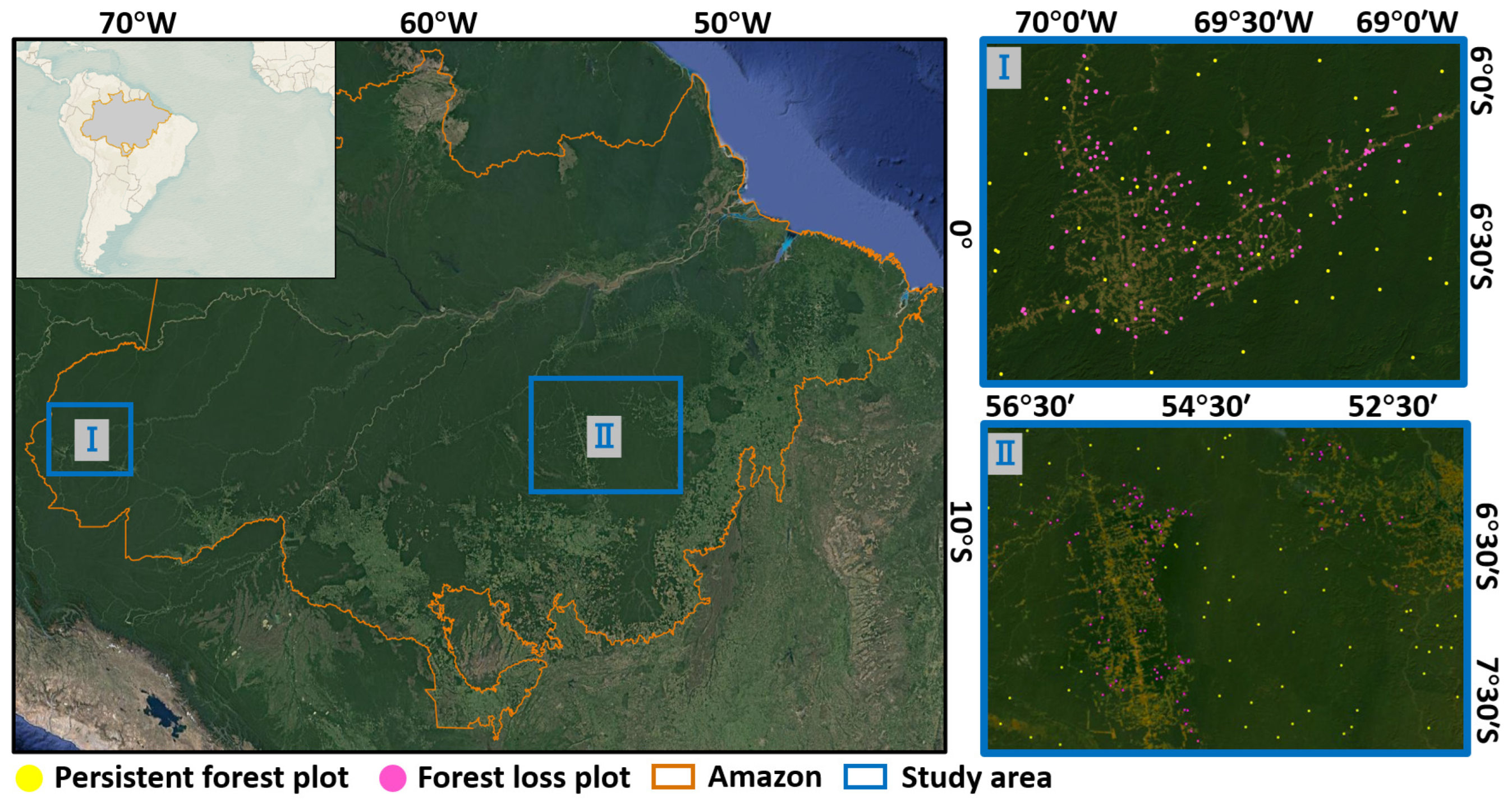
| Study area I in Amazon | 134 | 0.05 | −0.25 | 93.68% |
| Study area II in Amazon | 171 | 0.05 | −0.26 | 80.12% |
| Forest Loss | Persistent Forest | Total | ||
|---|---|---|---|---|
| Study area I in Amazon | PRODES | 43 | 37 | 80 |
| GEVI | 51 | 23 | 74 | |
| Study area II in Amazon | PRODES | 94 | 31 | 125 |
| GEVI | 58 | 19 | 77 | |
| Total | 246 | 110 | 356 | |
| Forest Loss | Persistent Forest | Producer’s Accuracy | User’s Accuracy | Overall Accuracy | Kappa | ||
|---|---|---|---|---|---|---|---|
| Study area I in Amazon | Forest loss in correct year | 137 | 13 | 91.33% | 90.13% | 86.00% | 0.78 |
| Persistent forest | 15 | 35 | 70.00% | 72.92% | |||
| Study area II in Amazon | Forest loss in correct year | 84 | 8 | 91.30% | 89.36% | 88.31% | 0.76 |
| Persistent forest | 10 | 52 | 83.87% | 86.67% |
| Loss in Correct Year | Persistent Forest | Producer’s Accuracy | User’s Accuracy | Overall Accuracy | Kappa | ||
|---|---|---|---|---|---|---|---|
| GLASS FFC CCDC | Forest loss in correct year | 84 | 8 | 91.30% | 89.36% | 88.31% | 0.76 |
| Persistent forest | 10 | 52 | 83.87% | 86.67% | |||
| MODIS VCF MODTrendr | Forest loss in correct year | 57 | 11 | 83.82% | 56.98% | 68.83% | 0.39 |
| Persistent forest | 37 | 49 | 60.64% | 81.67% | |||
| MODIS EVI CCDC | Forest loss in correct year | 34 | 6 | 85.00% | 36.17% | 57.14% | 0.25 |
| Persistent forest | 60 | 54 | 51.92% | 90.00% |
Disclaimer/Publisher’s Note: The statements, opinions and data contained in all publications are solely those of the individual author(s) and contributor(s) and not of MDPI and/or the editor(s). MDPI and/or the editor(s) disclaim responsibility for any injury to people or property resulting from any ideas, methods, instructions or products referred to in the content. |
© 2024 by the authors. Licensee MDPI, Basel, Switzerland. This article is an open access article distributed under the terms and conditions of the Creative Commons Attribution (CC BY) license (https://creativecommons.org/licenses/by/4.0/).
Share and Cite
Shi, W.; Zhao, X.; Yang, H.; Si, L.; Wang, Q.; Zhao, S.; Guo, Y. Generation of High Temporal Resolution Fractional Forest Cover Data and Its Application in Accurate Time Detection of Forest Loss. Remote Sens. 2024, 16, 2387. https://doi.org/10.3390/rs16132387
Shi W, Zhao X, Yang H, Si L, Wang Q, Zhao S, Guo Y. Generation of High Temporal Resolution Fractional Forest Cover Data and Its Application in Accurate Time Detection of Forest Loss. Remote Sensing. 2024; 16(13):2387. https://doi.org/10.3390/rs16132387
Chicago/Turabian StyleShi, Wenxi, Xiang Zhao, Hua Yang, Longping Si, Qian Wang, Siqing Zhao, and Yinkun Guo. 2024. "Generation of High Temporal Resolution Fractional Forest Cover Data and Its Application in Accurate Time Detection of Forest Loss" Remote Sensing 16, no. 13: 2387. https://doi.org/10.3390/rs16132387