Article

Developing a Semi-Automated Near-Coastal, Water Quality-Retrieval Process from Global Multi-Spectral Data: South-Eastern Australia

1
School of Civil Engineering, The University of Queensland, Brisbane, QLD 4072, Australia
2
School of the Environment, The University of Queensland, Brisbane, QLD 4072, Australia
*
Author to whom correspondence should be addressed.
Remote Sens. 2024, 16(13), 2389; https://doi.org/10.3390/rs16132389
Submission received: 7 April 2024 / Revised: 25 June 2024 / Accepted: 26 June 2024 / Published: 28 June 2024

Abstract

:
The estimation of water quality properties through satellite remote sensing relies on (1) the optical characteristics of the water body, (2) the resolutions (spatial, spectral, radiometric and temporal) of the sensor and (3) algorithm(s) applied. More than 80% of global water bodies fall under Case I (open ocean) waters, dominated by scattering and absorption associated with phytoplankton in the water column. Globally, previous studies show significant correlations between satellite-based retrieval methods and field measurements of absorbing and scattering constituents, while limited research from Australian coastal water bodies appears. This study presents a methodology to extract chlorophyll a properties from surface waters from near-coastal environments, within 2 km of coastline, in Tasmania, south-eastern Australia. We use general purpose, global, long-time series, multi-spectral satellite data, as opposed to ocean colour-specific sensor data. This approach may offer globally applicable tools for combining global satellite image archives with in situ field sensors for water quality monitoring. To enable applications from local to global scales, a cloud-based geospatial analysis workflow was developed and tested on several sites. This work represents the initial stage in developing a semi-automated near-coastal water-quality workflow using easily accessed, fully corrected global multi-spectral datasets alongside large-scale computation and delivery capabilities. Our results indicated a strong correlation between the in situ chlorophyll concentration data and blue-green band ratios from the multi-spectral sensor. In line with published research, environment-specific empirical models exhibited the highest correlations between in situ and satellite measurements, underscoring the importance of tailoring models to specific coastal waters. Our findings may provide the basis for developing this workflow for other sites in Australia. We acknowledge the use of general purpose multi-spectral data such as the Sentinel-2 and Landsat Series, their corrections and algorithms may not be as accurate and precise as ocean colour satellites. The data we are using are more readily accessible and also have true global coverage with global historic archives and regular, global collection will continue at least 10 years in the future. Regardless of sensor specifications, the retrieval method relies on localised algorithm calibration and validation using in situ measurements, which demonstrates close-to-realistic outputs. We hope this approach enables future applications to also consider these globally accessible and regularly updated datasets that are suited to coastal environments.

1. Introduction and Background

Monitoring coastal water quality presents significant challenges due to the dynamic nature of coastal water bodies influenced by factors such as wind, waves, currents and tides, which can change over short time scales, e.g., hours. Water quality, in this context, refers to the optical properties of water, determined by the concentration of suspended and dissolved organic and inorganic materials. Properties of organic and inorganic materials can be measured through remote sensing techniques, estimating parameters such as phytoplankton concentration, total suspended solids (TSS) and yellow substances including coloured dissolved organic matter (CDOM) [1,2,3,4,5,6]. Globally, in remote sensing applications water bodies are classified into two categories: Case I and Case II waters [7]. Case I waters are characterised by suspended organic material originating from phytoplankton biomass, and primarily occurring in open oceans and some coastal waters. As the concentration of chlorophyll increases, these waters show a prominent absorption peak at approximately 440 nm and a shift in the reflectance peak from the blue region (in clear waters) towards the green region at around 570 nm, due to increased pigment concentration [8]. On the other hand, Case II waters encompass types of water bodies dominated by high concentrations of inorganic particles and CDOM, typically found in terrestrial and estuarine water bodies, lakes, streams and rivers (Figure 1). Coastal and estuarine water bodies, which are the focus of this work, have a highly spatially and temporally dynamic mix of Case I and II waters. Remote sensing observations are influenced by the combination of these components, as suspended and dissolved materials absorb, scatter and transmit sunlight differently. The impacts of these on absorption and scattering processes are able to be measured from optical remote sensing (Figure 1), where coastal water bodies will primarily occupy the space in the lower portion of the ternary diagram.
Collecting in situ data on water quality parameters, in the form of concentrations of suspended or dissolved organic and inorganic constituents, often entails the use of complex instrumentation and requires skilled personnel. Examples of these techniques include direct water sampling and subsequent laboratory spectro-photometry and other analyses of sampled materials, as well as the deployment of optical instruments to measure spectral absorption, scattering and transmission [10]. Deploying these methods and analysing results can be logistically challenging and time-consuming. In some cases, these approaches may be impractical for achieving repeated, appropriately detailed spatial coverage of extensive areas at scales suitable for managing in-water operations, such as aquaculture. Satellite and airborne remote sensing, using appropriate data and processing algorithms, potentially offer solutions to measure, map and monitor biophysical properties of water bodies over a range of spatial and temporal scales, ranging from local sites ( 10 4 sq.m) to global, and at fine levels of spatial detail (e.g., 5 m–10 m image pixel). General purpose, multi-spectral satellite image data, such as from the Sentinel-2 [11,12] and Landsat 8–9 [13,14] satellites and now higher spatial resolution small-satellite constellations such as Planet’s Super Doves [15], offer potential for measurement and mapping of water quality parameters. Although the spectral band positions and radiometric sensitivity of these data are not optimal for measuring absorption and scattering properties in water bodies, their pixel sizes (5–30 m), global coverage and acquisition frequency (daily to every 16 days), make them highly suitable for near-coastal environments measurements.
We acknowledge there are critical trade-offs in remote sensing of water quality in highly spatially and temporally dynamic coastal environments. The main aim of this paper is to demonstrate what is possible as a starting point for building regional, continental and global systems from these data. It is worth noting that current approaches produce accurate remote sensing estimates of terrestrial and atmospheric bio-physical processes began with similar imperfect datasets. This underlines the importance of persevering in advancing our capabilities rather than discarding them prematurely.

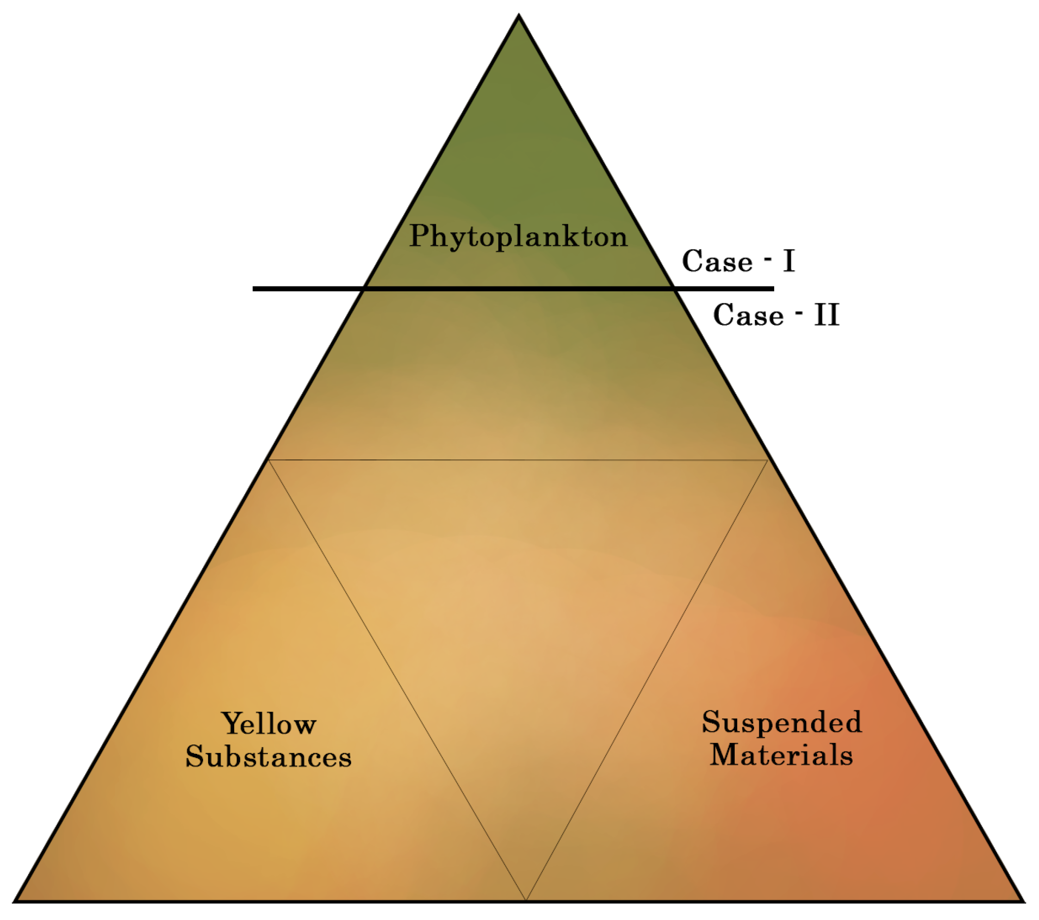
1.1. Water Quality-Estimation Approaches from Satellite Multi-Spectral Data

Phytoplankton composition, abundance and biomass in any given water body are key indicators of water quality. Chlorophyll a/b are the primary photosynthetic pigments in phytoplankton. Measurements of reflected sunlight from the surface of water bodies by airborne and satellite systems are used to estimate chlorophyll a/b concentrations and the amount of phytoplankton [16]. The concentration of chlorophyll a serves as a fundamental indicator of overall water quality, whether it pertains to aquaculture or the general health of aquatic ecosystems. Researchers have adopted various methods to quantify water quality parameters in diverse environmental settings. Empirical and semi-analytical models have been developed to enable the precise mapping of surface water chlorophyll concentration [17]. These models enhance our understanding of water quality dynamics and facilitating effective monitoring practices [1,3,18,19,20,21,22,23,24,25]. There have been recent advances in our abilities to access fine spatial scale (<10 m pixels), which are fully corrected for geometric, radiometric, atmospheric and surface reflectance factors. These high-quality and consistent satellite image data are available at global scales, yet retain local scale detail. Coupled with improved data-storage and -processing capabilities, these developments facilitate the creation and dissemination of new environmental-monitoring capabilities ranging from continental to global scales [26,27]. Mapping and monitoring of coastal water quality parameters like chlorophyll a/b is one of these capabilities that can be developed. This is despite the lack of ideal satellite data for global, daily to weekly coastal and estuarine applications [3,7,12,18,20,28,29,30,31,32,33,34,35,36,37,38,39]. This work is the first step in building an approach using publicly accessible, global coverage, frequently acquired, multi-spectral data to estimate and monitor a commonly used water quality metric, chlorophyll a.
Traditionally, the calculation of chlorophyll a (Chl-a) concentration in open ocean waters, classified as Case I waters, relies on the blue and green portion of the electromagnetic spectrum [7,8,32]. However, in turbid coastal waters, these bands are not suitable for accurately quantifying Chl-a concentration due to the overlapping absorption by CDOM. In inland water bodies characterised by high turbidity, e.g., suspended sediment load (Case II waters), a prominent absorption peak is observed around 685–700 nm [2,4,40,41], resulting from the combined effect of fluorescence and phytoplankton pigments. Conversely, in frequently clear, but usually mixed coastal and estuarine waters where most aquaculture operations are conducted, the absorption peak is relatively small, and the overall chlorophyll concentration is typically below 3 mg/m3 or equivalent to 3 μg/L [42]. Leveraging the principles of bio-optical theory, band combinations and algebraic manipulation can be employed to estimate bio-physical properties using a range of empirical or more deterministic approaches. It is crucial to identify the appropriate band combinations, as the absorption peak in the water column varies based on its inherent optical properties (IOPs). In shallow coastal near-shore areas (depth < 20 m), where waters can range from clear to turbid, additional bio-optically active constituents are often present. Even when these constituents are not present, in optically shallow waters, bottom reflectance including seagrass, a potential confounding source of Chl-a pigment signal, contributes significantly to the satellite-measured signals [3,7]. Hence, it is imperative to characterise and understand the environment to be mapped as much as possible before developing an appropriate satellite-based water quality mapping application. Continuous in situ monitoring of water quality parameters using widely available in-water sensors can offer accurate and temporally dense streams of near real-time information at specific points, aiding in the detection of any potential threats to aquaculture, such as harmful algae blooms [2,3,36,42,43,44]. However, it is essential to acknowledge that these in-water sensors require specialised personnel and techniques for installation, maintenance and data interpretation. They are susceptible to issues such as biofouling and environmental or technical damage, requiring periodic calibrations and expensive upkeep.
In contrast, satellite-based methods may present a more cost-effective long-term solution, if lower measurement accuracy and less temporally dense data are suitable for the application. Satellite monitoring enables capture of larger regions compared to single location in situ sensors. By understanding the optical properties over the areas to be mapped and monitored, selecting appropriate data and employing suitable mapping techniques, we can specify an appropriate capability to measure and monitor relevant water quality parameters, detect anomalies and mitigate potential risks to aquaculture operations. Timely and accurate assessment of water conditions is vital for ensuring the health and sustainability of aquatic environments and supporting the growth of aquaculture industries. A primary reason for pursuing the work presented herein is the ability to access regularly updated and corrected, global coverage satellite data streams in a processing and delivery environment that allows the development of a preliminary water quality monitoring approach. The data may not be ideal, but the infrastructure and processing capabilities can compensate to some extent.
The process commonly used to estimate water quality parameters in each satellite image pixel at wavelength ( λ ) is as follows, it relies on the surface remote-sensing reflectance value R( λ ) and the IOPs of the water bodies and can be expressed as:
R ( λ ) = f · b b ( λ ) a ( λ ) + b b ( λ )
where bb( λ ) is the back-scattering coefficient, a( λ ) denotes the total absorption coefficient and the coefficient factor f is primarily dependent on the angle of the incident light. The absorption coefficient can be further broken down into the composition of four factors including CDOM, non-algae particles (NAP), phytoplankton concentration aph( λ ) and pure water aw( λ ) [29,35,42].
a ( λ ) = a CDOM ( λ ) + a ph ( λ ) + a NAP ( λ ) + a w ( λ )
Understanding the retrieval process is crucial, as the behaviour of light varies depending on the inherent optical properties of the water. Previously, both blue-green and red-NIR band combinations have been utilised for Chl-a estimation. While the blue-green model accurately estimated chlorophyll concentration in some coastal waters, it tended to overestimate values in near-shore areas with highly turbid and CDOM-dominated waters [16]. Similarly, the red-NIR band approach failed in open water scenarios, as it did not receive sufficient signal reflected back to the sensors. Therefore, re-parameterisation becomes necessary, taking into account the characteristics of the specific water column [7,45]. Generally, the reflectance peak becomes more pronounced due to the presence of the fluorescence component of phytoplankton reflectance, aligning with the local minimum of the absorption coefficient resulting from the intersection of phytoplankton and water absorption spectra [5,40,42]. In open oceanic waters where phytoplankton dominates, the magnitude of 700 nm peak is relatively smaller. These distinctions underscore the necessity of adapting retrieval models and parameterisation techniques to specific water conditions. By considering the unique optical properties and variations within different water types, we can enhance the accuracy and reliability of chlorophyll extraction methods. This enables us to derive more precise information about the chlorophyll concentration and its distribution, contributing to a better understanding of water quality dynamics and ecosystem health.
Several versions of a global, ocean colour, polynomial algorithm (OC2, OC3 and OC4) have been developed by [38]. The algorithm, represented by (Equation (3)), is available on NASA’s ocean colour website (https://oceancolor.gsfc.nasa.gov/ (accessed on 4 April 2023)). It is specifically designed to estimate chlorophyll concentration in water bodies using sensors capable of capturing information within the wavelength range of 443 nm, 489 nm and 510 nm to approximately 555 nm of the electromagnetic spectrum, in cases where the chlorophyll concentration exceeds 0.2 mg/m3. Originally, the blue-green ratio method was developed for MODIS and SeaWiFS sensors for the retrieval process of chlorophyll a [46,47,48,49]. These algorithms are primarily tailored for Case I waters, where CDOM levels are relatively low. However, in CDOM-dominated waters, such algorithms may require additional processing steps or identifying the correct band ratios to account for the influence of CDOM on the remote sensing signal [50]. One approach could involve integrating multiple spectral bands to minimise the effect of CDOM and improve the accuracy of chlorophyll a estimates in such environments, particularly when in situ data is not available or when direct links between the two datasets cannot be established. This can be achieved by testing and establishing the band correlations through in situ data [51]. In this context of model development, it is essential to consider homogeneous pixels, particularly when the optical properties are highly sensitive to the reflected light. Minor changes in reflectance spectra can lead to under- or over-estimation of the overall chlorophyll concentration.
log 10 Chl-a = a 0 + i = 0 4 a i · log 10 R λ 1 R λ 2 i
Chl- a Hu = R λ 2 R λ 1 + λ 2 λ 1 λ 3 λ 1 · ( R λ 3 R λ 1 )
where the λ 1 is the maximum reflectance value between 443 nm and 520 nm, the λ 2 is located around 547 nm to 561 nm and λ 3 is positioned around 670 nm of the spectrum. For mapping open ocean water with relatively low chlorophyll concentration, multiple sensor-specific coefficients ( a 0 a 4 ) have been developed using in situ data collected through NASA’s bio-optical Marine Algorithm Dataset (NOMAD) [52,53]. Several researchers have used these measurements as a basis to adjust their chlorophyll-estimation methods and improve the accuracy of estimates. The last NOMAD data update was in July 2008, caution should be exercised in selecting and applying these data in any model, as the cessation of NOMAD updates in 2008 may indicate a temporal gap in coverage, impacting the representation of changes in water dynamics. Given the dynamic nature of water bodies, it is crucial to continue monitoring beyond 2008 to capture significant changes and maintain reliability of chlorophyll-estimation models [54]. Another option to develop locally specific chlorophyll-estimation models is to use regularly updated in situ data collection within the area being monitored. As an example, in global ocean monitoring studies, fourth-order polynomial OCx algorithms have provided accurate results [19,46]. Additionally, Hu et al. [55] developed the colour index algorithm (Equation (4)) specifically for areas where Chl-a concentration is less than 0.15 mg/m3.
This study develops a site-specific model for quantifying surface chlorophyll a concentrations in Tasmanian waters, a mid-latitude, temperate coastal region of the southern ocean, located between 40° and 45° south. The objective of this model development is to provide a proof of concept for satellite-based time-series measurements of chlorophyll a concentrations to inform development and management of specific aquaculture operations in the area. This requires the use of satellite multi-spectral data, which possess the following: (1) appropriate bands; (2) suitable spatial resolution to capture near-shore areas without introducing mixed pixels with land; and (3) are collected periodically to monitor changes in these environments. While Chl-a is a key component for modelling primary productivity in aquatic ecosystems, CDOM presents a significant challenge in Tasmania coastal waters due to its dominance in light absorption [50,56]. This dominance can interfere with chlorophyll detection, especially after heavy rainfall. CDOM and chlorophyll can exhibit overlapping spectral signatures, particularly in the blue-green wavelength range commonly used for chlorophyll detection [57]. Due to this overlap, it can be challenging to isolate the signal from chlorophyll when measuring it in the presence of CDOM. This is especially true in coastal waters where CDOM concentrations can be high due to terrestrial inputs from rivers and runoff. We acknowledge our approach may not meet the required data standards for scientific ocean colour work, but present it as a proof of concept that can be modified and scaled to new data as it becomes available. This is how the global vegetation structure and process modelling communities started, and scaled-up terrestrial ecosystem models for estimating a range of physiological parameters, leading to estimates of primary production [58].

1.2. Aims

The primary aim of this work is to develop, apply and validate a method to estimate chlorophyll a concentration from a global multi-spectral satellite archive and ongoing collection that has suitable spatial and temporal scales to work in coastal and estuarine areas. In this study, NASA’s USGS Landsat 8 level-2 analysis-ready data (ARD) that are orthorectified, radiometrically and atmospherically corrected [26,59], were employed to extract water quality information from several temperate coastal estuarine aquaculture sites in Tasmania, Australia. Individual bands were further adjusted with scaling factors and offsets according to the metadata. To establish and assess the relationships between field-measured water parameters and reflectance as measured in each pixel of the Landsat archive, satellite data were obtained from Google Earth Engine (GEE) and in situ data from 57 different survey locations along the east coast of Tasmania, collected in September 2022.
To achieve our aims, an approach was developed and tested using the GEE global satellite data-storage and -processing capability, and its Landsat archive, along with in situ data for calibration and validation. We acknowledge that data from the Landsat 8 sensors are not specifically designed for ocean colour measurements. However, they offer ongoing multi-decadal global coverage at spatial and temporal scales suited to coastal monitoring. Satellite estimates of chlorophyll a concentration are then matched and compared to locally captured in situ data, providing a limited assessment of the accuracy of our methods.

2. Data and Methodology

In this study, NASA’s USGS Landsat 8 level-2 analysis-ready data (ARD) were employed to extract water quality information from several temperate coastal estuarine aquaculture sites in Tasmania, Australia. To establish and assess the relationships between field-measured water quality parameters and reflectance as measured in each pixel of the Landsat archive, satellite imagery was obtained from GEE and in situ data from 57 different survey locations along the east coast of Tasmania were collected in September 2022 (Figure 2). The process used to estimate and map chlorophyll a and then validate the estimates is outlined in Figure 3.

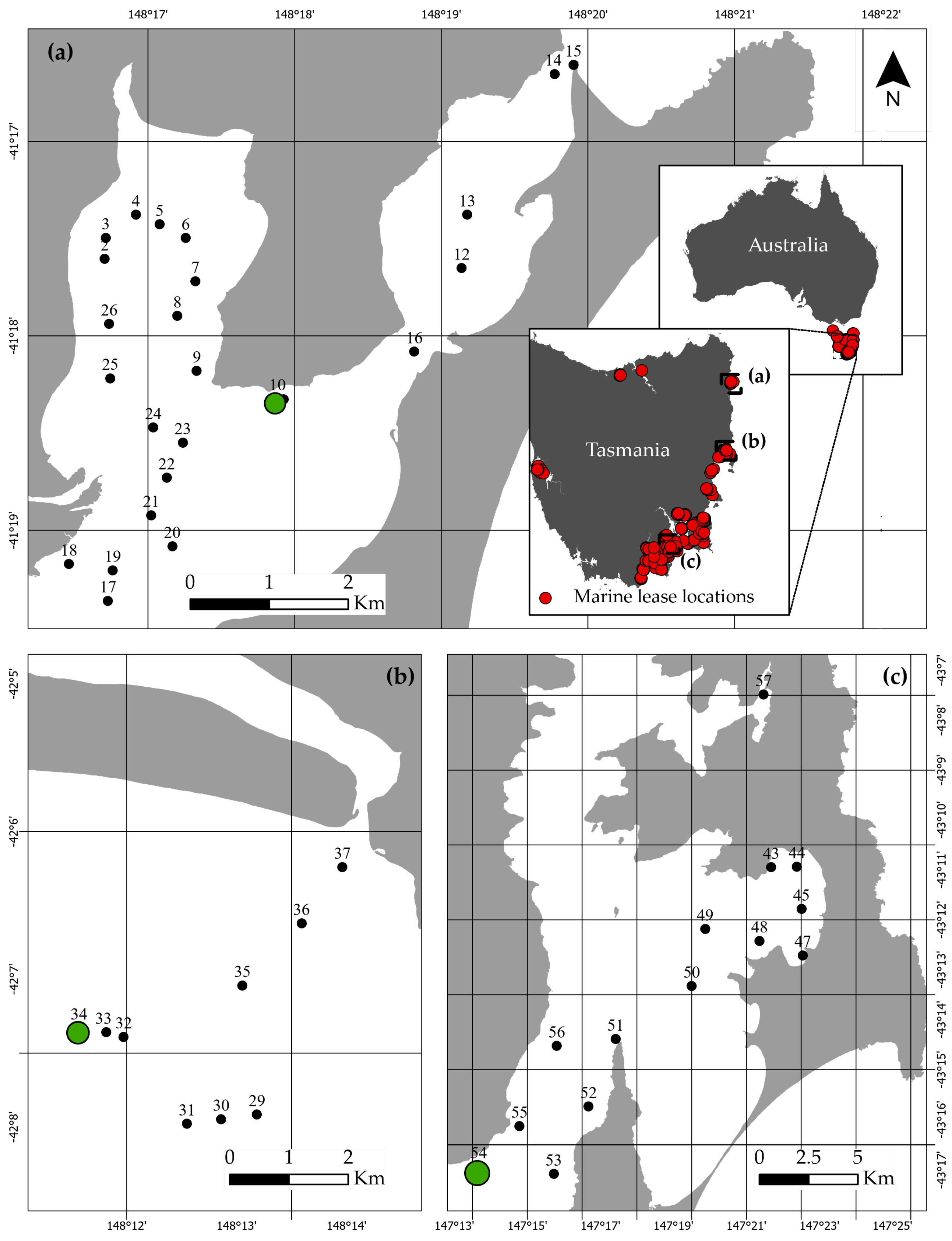
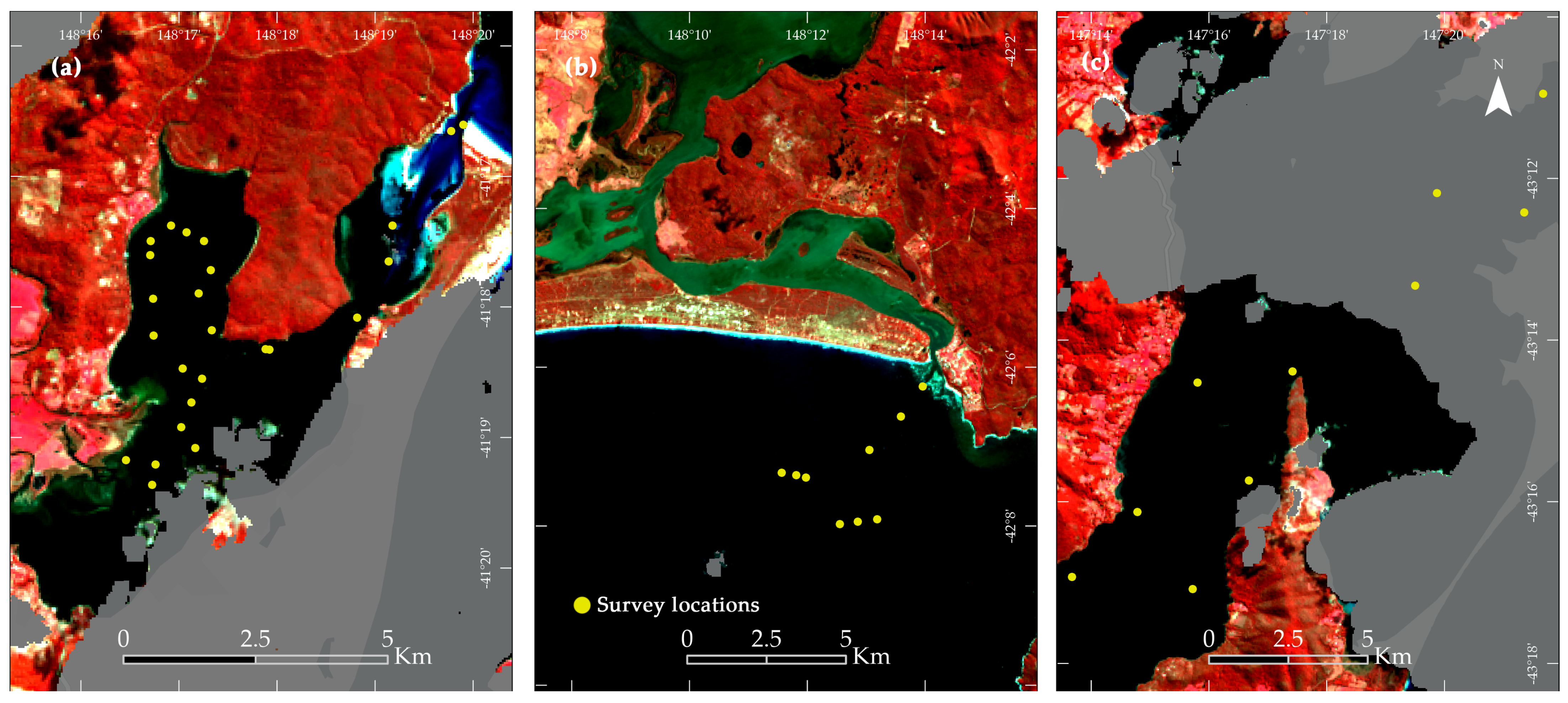
2.1. Field Data Collection

Tasmania is one of the largest producers of salmonids (salmon and trout) in Australia, supplying over 90% of the country’s Atlantic salmon, with a market value exceeding AUD 1 billion [61]. In addition, Tasmania cultivates a substantial quantity of Pacific Oysters, Angasi Oysters and other shellfish. According to 2022 statistics, Tasmania is home to approximately 44 local farmers who collectively produce oysters valued at around AUD 39 million [62]. The demand for seafood, both in the domestic and international markets, has witnessed a substantial increase in recent decades. It is predicted that aquaculture operations will account for more than half of the global fish production for human consumption in the future [63]. Effective monitoring is essential to enable the management of these sensitive and critical environments to ensure sustainable farming practices and minimal environmental damage can be maintained.
In Tasmanian waters alone, there are over 200 aquaculture leases [60], highlighting the significant scale and importance of the industry. This project focuses on three locations along the east coast: St. Helens (STH), Great Oyster Bay (GOB) and Bruny Island (BNI) (Figure 2). These locations were carefully chosen as representative sites for the study. Bruny Island hosts a variety of aquaculture operations, encompassing salmon, trout and shellfish farming. In contrast, STH and GOB are primarily focused on shellfish farming activities. The numbered locations depicted in Figure 2 indicate where samples were collected, enabling a comprehensive assessment of surface chlorophyll a concentrations in these specific areas.
In October 2021, at the Bruny Island site near lease 116 (Figure 2c: location 48), a Xylem Exo 2, a multi-parameter water quality sonde (More information available at https://www.xylem-analytics.com.au/productsdetail.php?YSI-EXO2-Multiparameter-Sonde-8 (accessed on 8 September 2021)), along with a DB600 real-time buoy (More information available at https://www.xylem-analytics.com.au/productsdetail.php?DB600-Real-Time-Data-Buoy-368 (accessed on 8 September 2021)) were deployed. The sonde was positioned at a depth of 0.6 m below the sea surface and collected samples at 10-minute intervals. This sensor suite enables the measurement of various water quality parameters including chlorophyll a concentration (mg/m3) using fluorescence, as well as turbidity, salinity and water temperature. To prevent biofouling, a wiper on the sensor is activated every 15 min. The buoy’s solar power capabilities ensure continuous and uninterrupted data collection. The collected data can be easily accessed through the eagle.io platform or integrated into the extraction model for comparison with satellite data. Regular sensor cleaning procedures are implemented to prevent biofouling, and calibration procedures are conducted to maintain the precision of the measurements. To capture water properties at different depths in the other two sites, STH and GOB, a handheld sonde was used to collect samples at each designated location (refer to Figure 2) at different depths. Subsequently, the data were retrieved from the instrument for further analysis.

2.2. Satellite and Field Data to Estimate Chlorophyll a Concentration

The two most critical sources of information needed for aquaculture facilities, to enable them to determine short-term (day-week) and longer-term (months) water quality management, are temperature and water quality parameters, which include the measurement of organic and other suspended or dissolved materials in the water. Ideally, these data encompass both surface and sub-surface points, allowing for estimation through various sensing methods such as in situ, drone, airborne and satellite sensors, which measure how sunlight interacts with suspended and dissolved constituents in the water. Extensive empirical and deterministic methods have been developed to extract the optical properties of the near-surface waters (Figure 3). By utilising empirical models (Equation (3)), globally accessible higher spatial resolution multi-spectral data, and in situ data for our three study sites, this work demonstrates a method for mapping near-shore water quality parameters for potential use in monitoring aquaculture operations.
In this study, Landsat 8 (L8) imagery with a spatial resolution of 30 m was employed to extract surface water properties due to its suitable pixel size, repeat frequency, global coverage and a full archive from Landsat 1–9, dating back to 1972. Although not tailored for ocean colour observations, L8 has limitations in radiometric calibration, accurate atmospheric correction and potentially lower signal-to-noise ratio or gain for coastal and marine environments. Nonetheless, its inclusion of relatively narrow bands in appropriate spectral regions makes it suitable for ocean colour applications [64,65]. As noted in earlier sections, we are using L8 because it is collected at spatial and temporal resolutions suited to coastal nearshore waters, and its spectral bands are sufficient but not optimal for coastal water quality. Other sensors specifically developed for ocean colour monitoring, such as MODIS, Sentinel-3, VIIRS and SeaWiFS, with spatial resolutions of 1000 m, 300 m, 750 m and 1100 m, respectively, were deemed unsuitable for this study due to their limited spatial resolution for resolving coastal water bodies where aquaculture operations are taking place. Given that most aquaculture operations occur near the shore, typically within a range of 50 m to 1 km, the use of sensors with higher spatial resolution becomes crucial. The presence of overlapping or mixed pixels with land in near-shore areas can also lead to inaccuracies in the estimation of surface chlorophyll concentration. Therefore, L8, with its moderate spatial resolution, provided a suitable compromise between data availability and the ability to capture detailed information in the near-shore regions of interest.

2.3. Extract Data from Satellite Images at Field Study Sites to Link with In Situ Data

To enable the development and validation of empirical models to estimate chlorophyll a concentration in the next section, a process was established to extract L8 surface reflectance to match with field measurements at each site. This process required matching spatial scales of field and satellite sampling and time periods of sampling as close as possible. The process of extracting L8 pixel reflectance at each sample site was as follows:
One of the primary criteria for selecting optimal sampling locations was the presence of existing aquaculture sites. Additionally, we strategically chose areas that would minimise mixed pixel information, a consideration crucial for the satellite sensor’s spatial resolution. As a result, locations were identified at a minimum distance of 30 m from the land or coast, a threshold aligned with the spatial resolution of Landsat 8. The careful selection of locations extended beyond geographical proximity, with a deliberate consideration of various bottom depths to ensure a representative sampling across the aquatic environment. While directly removing the effects of CDOM absorption in complex water systems remains a challenge, identifying robust band ratios with high correlation to true chlorophyll a concentrations can help minimise this confounding factor. We investigated various band-ratio algorithms using in situ chlorophyll a data to identify optimal combinations for establishing correlations between actual and satellite-derived Chl-a values. This approach enhances the reliability and applicability of the field measurements in capturing surface Chl-a dynamics in the chosen study areas.
It is crucial to note a distinct time gap between the actual survey date and the image capture date. As illustrated in Table 1, there is an approximate time gap of 2–3 days between the survey and the image capture. Additionally, some survey points were not captured by image pixels due to cloud coverage. Hence, establishing a direct match for each survey point to the corresponding image pixels from the same date remains challenging. Table 1 provides an overview of the survey dates, image acquisition dates and image details for each of the satellite images utilised in the development of the site-specific chlorophyll extraction model. Figure 4 presents a false-colour composite map illustrating the cloud-free areas overlaid with the field survey locations. The grey areas indicate where surface properties are masked due to the presence of clouds and shadows caused by the clouds. The end result is a series of field measurements and corresponding L8 pixel values in a table to build and evaluate models.
The handheld Exo 2 multi-parameter sensor was crucial for data collection at each survey site, capturing chlorophyll a values at specific surface locations and through the water column. Measurements in micrograms per liter (µg/L) were averaged across the top 1 m for comparison with satellite multi-spectral data. In contrast, satellite sensors capture pixels with 30 m × 30 m surface areas in surface reflectance values, offering an extensive yet somewhat averaged representation in mg/m3. While the reflectance values themselves are unit-less, the algorithms are calibrated using in situ measurements of chl-a concentrations, which are typically expressed in units of milligrams per cubic meter (mg/m3). This correlation underscores the satellite’s capability to capture information not just on the surface but, depending on the water column clarity, also extends to different depths based on how far each wavelength can penetrate. However, it is crucial to recognise specific nuances in the measurement process. Disturbances caused by the movement of the boat, and changes in water flow and other environmental factors, can introduce discrepancies in the actual surface chlorophyll values, as continuous movement can disrupt the water column and affect the distribution of chlorophyll a concentrations. These factors should be highlighted because they pose challenges in interpreting satellite-derived data, significantly impacting the precision of the measurements. This underscores the necessity for careful validation against in situ measurements taken by the handheld sensor.
Traditionally, the feature extraction process has involved manual downloading of satellite multi-spectral data to a local server, resulting in a series of manual image-processing tasks for each scene to extract surface information. This method requires significant storage capacity on local devices and is prone to human errors due to the repetitive nature of the tasks. In this project, an automated approach using a cloud platform has been developed to streamline the entire process. Google Earth Engine is utilised as a cloud computing platform, which leverages multi-petabyte global satellite image archives and geospatial datasets at various scales for spatial analysis [59,66,67]. Atmospherically and surface reflectance-corrected scenes representing Landsat 8 pixels at 30 m resolution are used to ensure the inclusion of homogeneous water pixels for further processing. These corrections are performed using the Land Surface Reflectance Code (LaSRC), which is applied to all Collection 2 Surface Reflectance (SR) products (Landsat 8 SR products are created with the Land Surface Reflectance Code (LaSRC). All Collection 2 SR products are created with a single-channel algorithm jointly created by the Rochester Institute of Technology (RIT) and the National Aeronautics and Space Administration (NASA) Jet Propulsion Laboratory (JPL) [68]). It should be noted that the effectiveness of atmospheric corrections designed for terrestrial environments, characterised by relatively higher brightness levels, may not be directly transferable to marine settings, where reflectance is considerably lower. However, such corrections facilitate the implementation of proof-of-concept demonstrations, as exemplified in this study. A total of 39 out of 57 survey location pixels were extracted for each individual surveyed location from the available Landsat 8 scenes, each with a spatial resolution of 30 m × 30 m. Survey locations were carefully selected to align with the sensor’s spatial resolution, ensuring that only homogeneous water pixels around the designated points were included for further image processing. Additionally, pixels containing clouds or shadows were excluded from the analysis to maintain data quality. Homogeneous pixels are essential for accurate extraction of surface information, as they facilitate more reliable assessments of water quality parameters and minimise potential errors in the analysis. In this study, samples were collected at various locations with different benthic depths, and at multiple depths at each locations, extending until reaching the benthic floor, as outlined in Appendix D, Table A1, to gain insight into the interaction between light and Tasmanian coastal waters. It should be noted that mapping Bruny Island proves to be challenging due to the high cloud coverage in the area. In the future, the utilisation of commercial satellites with high-resolution imagery and high temporal coverage can enable the capture of more cloud-free images.

2.4. Develop Models to Estimate Chlorophyll a Concentration from L8 Satellite Reflectance and Field Measurements

The initial step in our methodology involved using the blue-green empirical model to extract surface chlorophyll concentrations at three locations in Tasmanian waters. To assess the model’s performance, data from all surveyed sites were aggregated and input into the equation for evaluation. However, the results revealed sub-optimal correlations between in situ measurements and the satellite multi-spectral imagery. The sub-optimal correlations between datasets primarily stem from localised parameters, such as water turbidity, temperature, dissolved organic matter concentration and benthic characteristics, which significantly influence water column dynamics [69], as evidenced by numerous studies demonstrating correlations between these parameters and changes in water quality, ecological shifts and biological productivity [54,70]. These factors vary based on several environmental factors, including geographical locations and surroundings. These factors contribute to the observed discrepancies in chlorophyll concentration estimates. Consolidating data from all three sites (STH, GOB and BNI) revealed no correlation between the in situ and satellite data, indicating that significantly different bio-optically properties apply at each location.
Recognising the unique spectral signatures at each location, due to differences in the optical properties of each water body influenced by their position, size, oceanic-terrestrial inputs, we employed an individual location-wise empirical modelling approach. This individual location-wise approach revealed more meaningful and distinct correlations compared to the aggregate dataset. To enhance the model’s precision for surface chlorophyll extraction, we applied NASA’s OCx model, using a fourth-order polynomial model to scale the empirical model outputs and align them with the in situ data. This involved establishing location-specific regression coefficients.
The next phase involved applying individual regression coefficients to the refined model, and these site-specific coefficients were then integrated into the GEE algorithm. This integration facilitated the extraction of surface chlorophyll concentrations for each survey location, allowing for a detailed analysis of correlations and Root Mean Square Error (RMSE), while also evaluating the correlation between the extracted surface chlorophyll concentrations and in situ measurements. This approach aimed to enhance the model’s adaptability and provide a comprehensive understanding of surface chlorophyll dynamics at a local level.

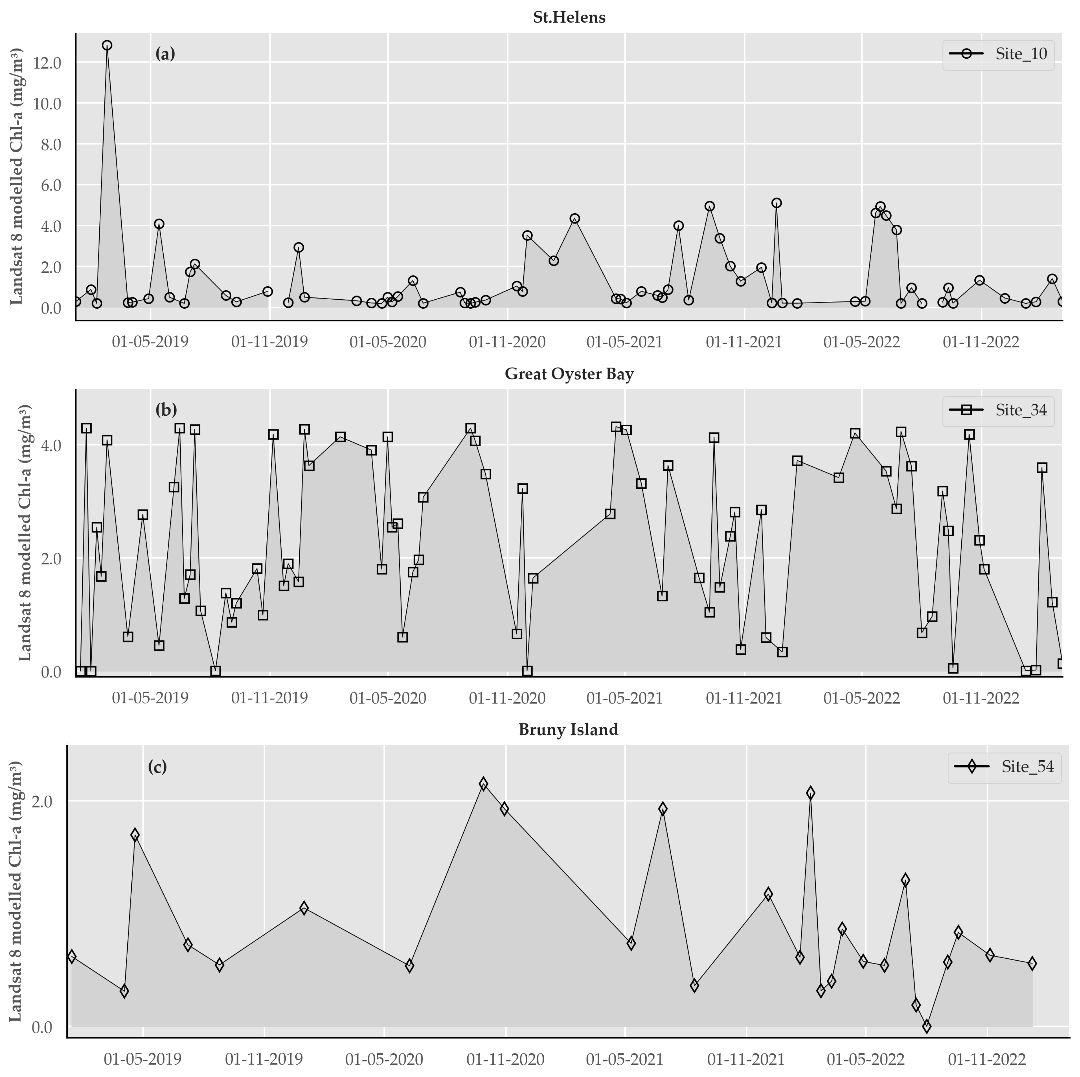
2.5. Produce Time-Series of Output Chlorophyll a Maps at Each Study Site

To demonstrate the effectiveness of the automated image-processing approach, a comprehensive time-series analysis was conducted for each of the 57 surveyed locations. A total of 389 individual scenes (STH—130, GOB—140 and BNI—119 scenes) spanning from 1 January 2019, to March 2023, were chosen and directly processed from the GEE server. The emphasis on at-surface reflectance values from satellite image data holds paramount importance for retrieving accurate estimates of absorption, scattering, transmission and related biophysical properties. For each of the three study sites over the 2019 to 2023 time period, individual scenes were masked based on cloud coverage, and data were carefully screened to ensure surface reflectance correction, exclude pixels containing clouds or cloud shadows and include only homogeneous pixels with water features. The outcome of this screening yielded specific satellite image datasets for each study site, STH—1344 pixels, GOB—643 pixels and BNI—171 pixels in total, distributed across the field survey locations, with each pixel representing a 30 m × 30 m area of the water surface. The workflow, operating directly on the Google server independent of the local server, facilitated the extraction of surface chlorophyll information based on optical properties. Site-specific parameters were integrated into the GEE model for automated extraction in each study area. This integration resulted in chlorophyll concentration maps ranging from 0 to 10 mg/m3, providing comprehensive insights into the spatio-temporal dynamics of surface chlorophyll across the study sites.

2.6. Validate Estimated Chlorophyll Levels against Field Data Not Used in Model Development

In the validation phase of our methodology, we assessed the performance of the site-specific model derived from field samples collected in September 2022. To achieve this, we utilised the stationary solar-powered buoy situated at Bruny Island, equipped with an in situ sensor, measuring chlorophyll a concentrations, to validate the time series and the model’s efficacy. The buoy has been regularly collecting information since October 2021, providing dataset suited for evaluation. It is crucial to acknowledge that establishing the model based on the time-series of a single point throughout the year may be insufficient. This limitation becomes evident when considering the extensive dataset captured through the stationary in situ sensor; despite its breadth, this single point dataset cannot adequately calibrate the model for the entire study region. The spatial correlation differs from temporal correlation due to the dynamic nature of the water column, which varies distinctly across different locations, necessitating a model that captures variations in data collected at diverse locations. To address this, the model was fitted with data variations from different locations and subsequently validated against a single location, leveraging the available dataset. Notably, one of the primary challenges encountered in this project revolves around the lack of historical datasets in the targeted regions. This emphasises the critical need for robust validation methods in time-series analysis and temporal correlations.
To test the reliability and applicability of our model, a second buoy with an identical sensor was strategically installed at a 4 m depth in Great Oyster Bay, at coordinates (148.210, −42.131), in May 2023. Table 2 displays the deployment dates and locations for both BNI and GOB in situ stationary buoys. This additional buoy augments our validation efforts by introducing a new location with its unique environmental dynamics.
In both the Bruny Island and Great Oyster Bay cases, we executed the model on the GEE server, employing individual site-specific parameters as outlined in our methodology (see Figure 3). This process enabled the extraction of cloud-free pixels with associated surface chlorophyll values. Subsequently, we compared these extracted values against the buoy data, which represented a single location with 30 m × 30 m Landsat pixels at each site for the same time match-up as the satellite overpass. The co-variance between these two datasets was then assessed, establishing correlations and RMSE metrics. This validation approach evaluated the model’s performance against the available buoy data and also assessed its generalizability and robustness across different geographical locations and environmental conditions. The comparison of model outputs with in situ buoy measurements serves as a critical step in ensuring the accuracy and reliability of our remote sensing methodology for mapping water surface chlorophyll concentrations.

3. Results

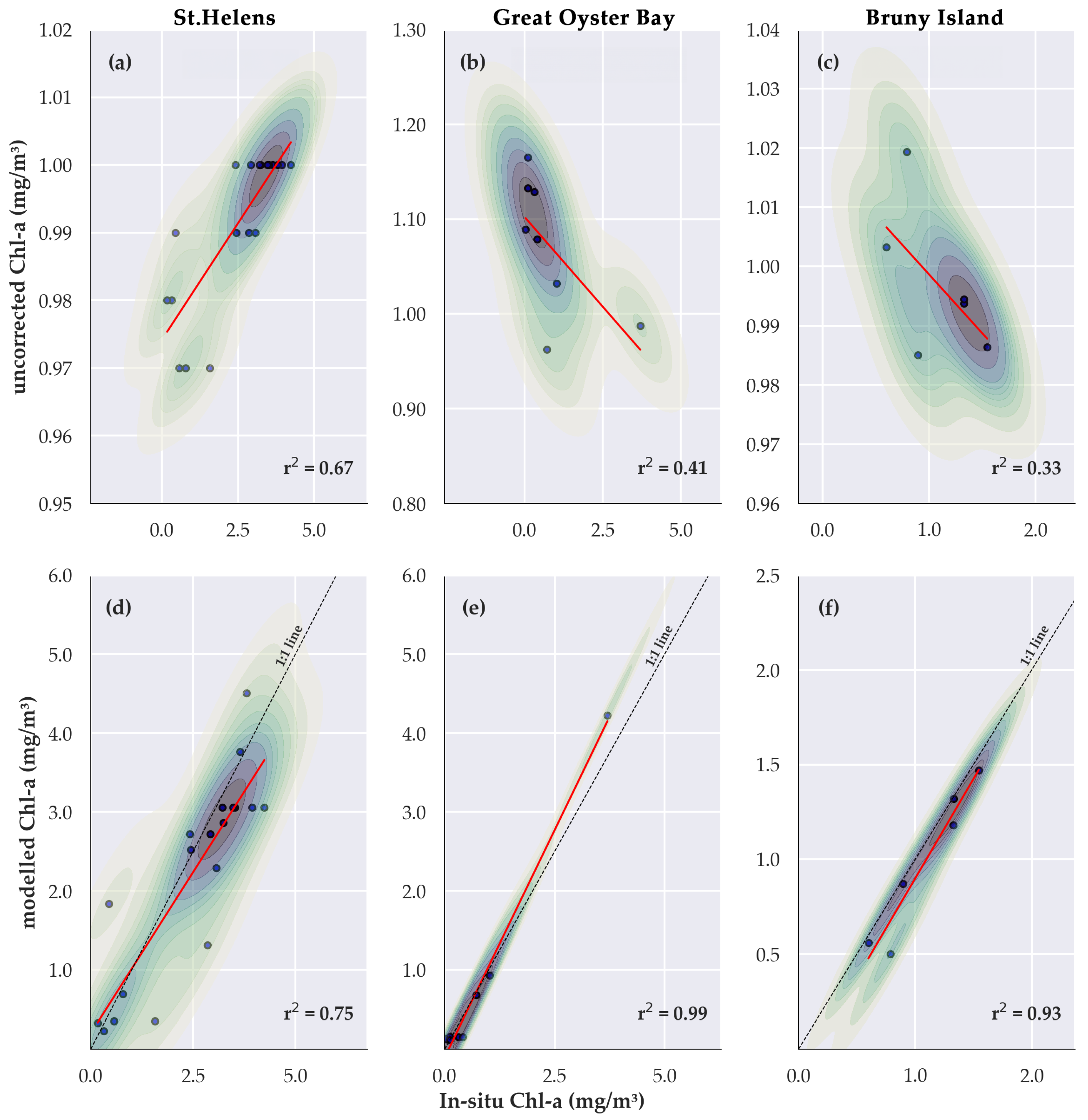
3.1. Linking Satellite and Field Data to Estimate Chlorophyll a Concentration

The model parameters were derived using the Blue-Green ratio and plotted against the field samples collected at surveyed locations, which encompass a range of bottom depths, from shallow waters to depths exceeding 20 m (Table 3). Findings obtained from Landsat 8 were compared against the in situ measurements, considering sites across varying benthic depths. Areas with a bottom depth shallower than 2 m were excluded to minimise potential spectral interference from benthic properties. Initial analysis revealed a correlation between modelled and observed chlorophyll data. Table 3 shows the base and derived correlations using the fourth-order polynomial equation, where the parameters a 0 a 4 of Equation (3) are derived from an automated process. The combined dataset for all regions exhibited a weaker correlation compared to the factors specific to individual sites. However, the site-specific model showed a stronger correlation between modelled and in situ data. Particularly, GOB (b) and BNI (c) sites displayed very strong correlations of 0.99 and 0.93, respectively, with RMSE of 0.22 and 0.14 between the samples. STH (a) site also exhibited a strong correlation of 0.75 (RMSE = 0.74 mg/m3) between satellite-derived and in situ datasets, as shown in Figure 5. The red line on the scatter plot represents a linear least squares fit, illustrating the overall relationship between the variables. The background contour plots show data point density, visualising the distribution and indicating areas with higher frequencies of occurrence. The denser the contours, the more data points are clustered in that region, highlighting the overall trend and variability within the dataset. It is important to highlight that St. Helens site (STH) is surrounded by land on almost all sides and has a complex water column around the bay, due to effects of surrounding topography and terrestrial inputs. This results in more variable water quality compared to open coastal waters.
Optically shallow sites are affected by bottom reflectance, which can extend to depths of up to 20 m in certain environments [71,72]. In some instances, depths shallower than 2 m are significantly affected by this. To mitigate the impact of bottom influence, we established a threshold to exclude areas where the bottom influence was visible. Despite the bottom influence in our three study areas exceeding beyond 2 m, depending on water clarity, we opted to apply a 2 m threshold in this analysis and excluded sites that did not meet this criterion. This threshold was adapted from a previous study conducted in coastal waters around Hainan Island, China [6]. Further analysis of the bottom threshold is warranted in future research, particularly tailored to specific environmental contexts.
Site-specific model parameters were applied to map chlorophyll a concentration across all three study sites through the automated model. This process allowed for a detailed spatial representation of chlorophyll a distribution, providing insights into the variations and trends across the surveyed areas shown in Figure 6. The incorporation of site-specific parameters ensured the accuracy and relevance of the generated chlorophyll a concentration map, enhancing the applicability of the model to capture the specific characteristics of each site. This semi-automated mapping approach may contribute to a more efficient and standardised assessment of chlorophyll a levels. This approach allows water quality dynamics in the surveyed regions to be estimated from easily accessible, higher spatial resolution satellite data suited to these coastal embayments. In most inshore aquaculture sites, the Chl-a concentration ranges between 0.2 and 2.0 mg/m3. Open water areas generally exhibit a concentration of around 0.2 mg/m3. The concentration increases near the river mouths and close to the land masses due to multiple terrestrial inputs such as sediments, nutrients and other chemicals.
Out of the 57 sample points, 33 were selected for analysis. These points were chosen to ensure they were free from pixels flagged by the quality information provided in the satellite metadata for the respective sites and dates. In our data screening algorithm, we implemented cloud, cirrus and cloud shadow masking using the QA_PIXEL catalogue to mitigate potential artefacts. However, some visible artefacts, particularly in Bruny Island (Figure 6c), persist. These anomalies may arise from factors such as incorrect metadata, limitations in shadow detection and sensor noise issues, which warrant further investigation to enhance the accuracy of our estimates. These factors play a crucial role and can impact the accuracy and reliability of the mapping process. Therefore, their presence and potential impact should be considered when designing mapping processes and interpreting the results. The initial testing of the model did not yield a strong correlation between field data and sensor-derived data in deeper waters. Applying a minimum water depth threshold of 2 m depth across all three study sites improved the model’s performance. Retrieving chlorophyll from coastal shallow waters with low concentration will continue to be challenging due to bottom effects. Further investigations might be required to optimise our methods for various water depths, particularly in shallower areas where bottom effects are more pronounced and in deeper waters (>30 m) to confirm the consistency of our approach and improve overall model reliability [6].
It is evident that a generalised model coefficient applicable to all regions may not be suitable for water quality monitoring from satellite data for aquaculture operations. Thus, the development of a location-based model is crucial, as it incorporates local in situ data to accurately extract surface water features and provide reliable results. Furthermore, it is essential to recognise that, while all three study areas remain predominantly clear waters, these regions may exhibit significant absorption of light due to the presence of CDOM and Chl-a. Consequently, the model coefficients developed for these environments may not be directly applicable to areas such as those near river mouths, which are characterised by elevated levels of CDOM and sediment concentrations.

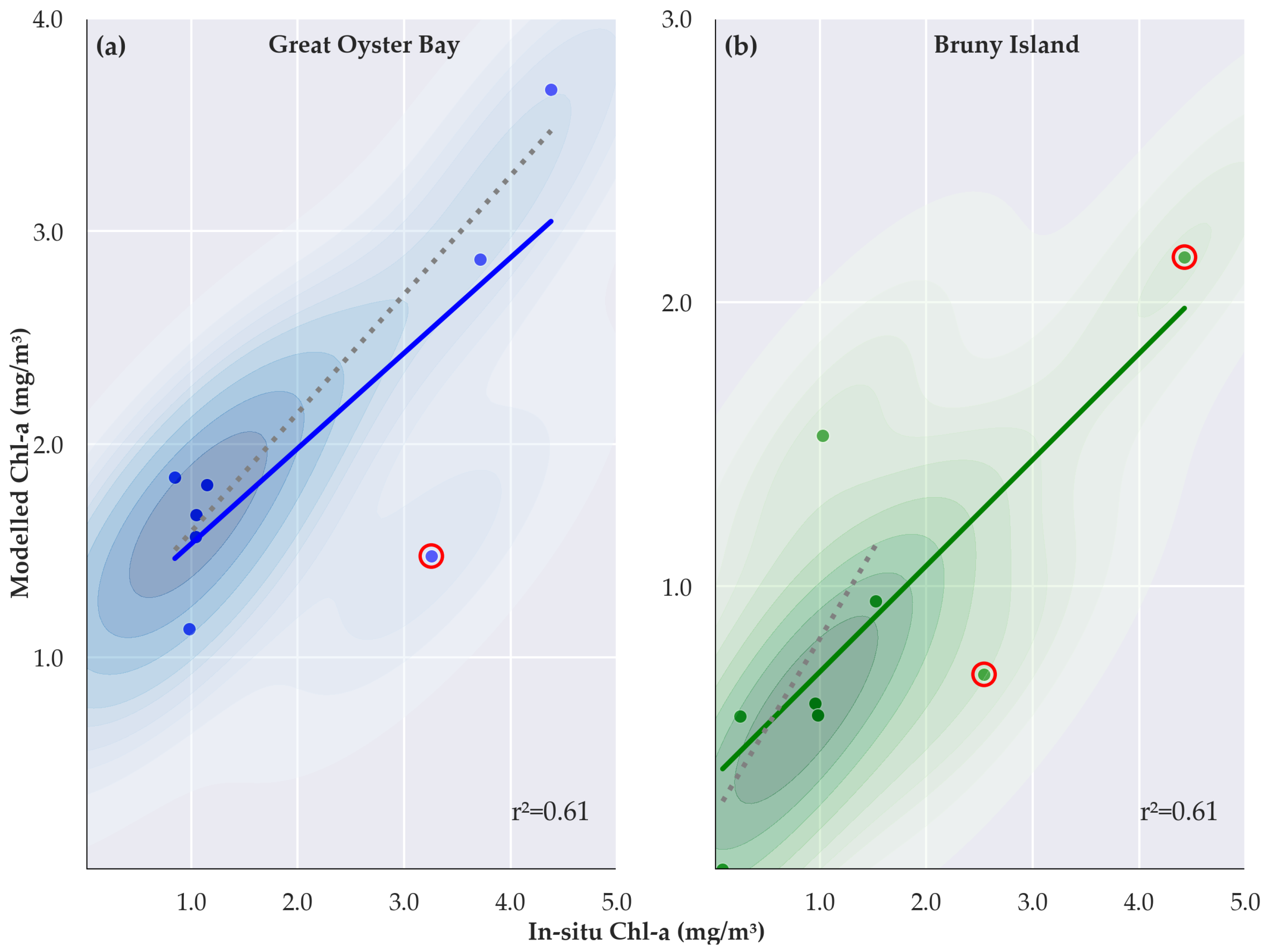
3.2. Validation of Estimate Chlorophyll a Concentration

The scatter plots in Figure 5 represent the correlation between the two-band model using Landsat 8 images and the corresponding in situ data. Figure 5a–c show the co-variation between in situ data and the initially derived Chl-a concentration resulting from the Blue-Green band ratio of Landsat 8 for the same location. The extracted chlorophyll values were significantly underestimated compared to the in situ values. To estimate site-based chlorophyll concentration, the site-specific modelled coefficients were then incorporated into the model. In Figure 5d–f, the y-axis values are the results for site-specific parameters using the fourth-order polynomial model, resulting in Chl-a concentrations closely aligned with range and distribution of the in situ measurements specific to each location. The STH sites had a large range of Chl-a values due to its complex embayment and impact of terrestrial sources, while GOB and BNI exhibited the more typical lower Chl-a concentration of coastal sites.
To further substantiate our validation efforts, Figure 7 illustrates a comparison plot of satellite-derived data with in situ observations at specific locations throughout the study period. As highlighted in Table 3, the sensor, located in GOB (Figure 7a), was only installed in May 2023, whereas the sensor in BNI (Figure 7b) has been operational since October 2021. For the purposes of this comparison, only cloud-free satellite observations were selected to ensure accurate temporal analysis within the designated period. This alignment underscores the challenge posed by the sporadic availability of cloud-free satellite images, emphasising one of the challenges inherent in using satellite remote sensing data for environmental monitoring in cloud-prone areas. A stringent criterion for cloud cover exclusion was uniformly applied to both the recently installed sensor in GOB and the longer-operational sensor in BNI. This criterion aimed to ensure a consistent and comparable dataset for subsequent analysis, emphasising the need to navigate limitations posed by cloud cover and shadows in satellite imagery. The equal count of cloud-free satellite pixels for both in situ sensors further highlights the challenges associated with obtaining high-quality, uncontaminated data for accurate assessments of surface chlorophyll concentrations.
The Chl-a-estimation model, tailored for site-specific applications and excluding areas with depths less than 2 m, was applied to each of the three study sites, as depicted in Figure 6. Through the time-series validation, both GOB and BNI exhibited notable positive co-variances, registering correlation coefficients of 0.615 and 0.614 respectively, as illustrated in Figure 7. These results underscored the model’s adeptness in capturing local nuances, thereby highlighting its capability and robustness in estimating surface chlorophyll concentrations through Landsat 8 data. The corresponding RMSE values in mg/m3 were measured at 0.22 and 1.09 for the aforementioned sites. In both plots, the grey dotted lines represent the regression line, excluding the outliers highlighted by red circles in Figure 7. These outliers predominantly correspond to instances where in situ Chl-a measurements were elevated compared to the lower estimations from the Landsat satellite data. A possible explanation for both of these is the difference in spatial sampling unit between the in situ sensor and the satellite sensor. The in situ sensor is positioned at a specific depth (4 m below the sea surface) for a singular point location, whereas the satellite multi-spectral sensor, obtains a signal from a 30 m × 30 m surface measurement. The significantly higher in situ measurement at each site may be present in the satellite data but has been averaged out due to satellite sensor pixel size and other sampling controls.
This disparity in sampling resolutions between in situ measurements and satellite retrievals highlights a significant limitation in the remote sensing estimation process. Our approach demonstrates where both in situ and satellite measurements reflect elevated Chl-a levels. However, it is crucial to identify situations where satellite and in situ measurements do not match, showing transitions from low to high or high to low Chl-a levels. This discrepancy indicates potential anomaly or error in either the in situ sensor readings or the satellite-based estimation method. Addressing this issue requires collecting additional data to verify the model parameters. One effective method is collecting transect data, capturing sub-pixel variations and establishing stronger statistically significant correlations between in situ measurements at a sub-pixel level and satellite measurements at a single pixel level. This proactive approach ensures a more precise and adaptive strategy for safeguarding water quality within aquaculture settings. Recognising and addressing these Chl-a anomalies is essential, not only for immediate interventions but also for maintaining the long-term health and resilience of aquatic ecosystems critical to aquaculture activities.

4. Discussion

This section interprets spatial-temporal variations observed in our chlorophyll a estimations, within and between our designated study sites. Our findings also emphasise needs for enhanced accessibility to ocean colour data and water quality calibration and validation datasets. The model we formulated and implemented across three Tasmanian coastal areas, utilising the blue-green reflectance ratio derived from Landsat 8 imagery linked to in situ samples, produced accurate estimations of Chl-a concentration. Specifically, these estimations encompassed a coastal embayment, namely St Helens, as well as two expansive open-coast locations, Great Oyster Bay and Bruny Island, where the tidal range reaches almost 3.5 m [73]. The model yielded more precise Chl-a estimates in regions characterised by open waters, with reduced levels of suspended and dissolved organic and inorganic particulates [13]. Figure 8 presents the time-series data for Chl-a values derived from Landsat 8 archive using the blue-green model, calibrated with individual in situ derived model coefficients. The data cover an extensive three-year period and were collected at near bi-weekly intervals. Each unique symbol corresponds to a specific Chl-a measurement extracted from a designated survey location, as elaborated upon in Figure 2.
The Chl-a estimates across our three field sites, STH, GOB and BNI, revealed distinct spatial and temporal patterns at each location throughout the study period. These variations arise from a confluence of site-specific factors, including localised environmental processes, and bathymetric complexities. STH, characterised by its complex water column properties, presented a significant disparity in Chl-a concentrations mostly influenced by the complex currents and nutrient dynamics. Notably, the Landsat 8-based two-band algorithm exhibits limitations in representing such complex aquatic systems [74], and collecting more in situ data over an extended period is necessary to enhance the model’s reliability. Accurately retrieving water quality information from complex water bodies poses challenges, primarily due to their unique optical properties. Moreover, these challenges vary significantly across different aquatic environments, suggesting that a uniform model applied across diverse water bodies may not consistently produce accurate results [16,75]. In contrast, GOB and BNI exhibited a different trend, often characterised by lower Chl-a concentrations compared to STH, where chlorophyll level is comparatively higher. The differences in coastal dynamics and bathymetric characteristics for each site likely play a significant role in shaping these Chl-a patterns. Our analyses underscores the need for integrating site-specific factors in models. This approach allows the complex relationships between geographic, hydrodynamic and bathymetric components that collectively define the distinctiveness of each coastal area and its landscape to be included.
Examining the temporal variations in Chl-a estimates across our study locations, St. Helens, Great Oyster Bay and Bruny Island, revealed distinctive patterns in Chl-a concentrations over the study duration. STH exhibited peaks in Chl-a levels during the winter months of July and August, potentially due to increased runoff from the George River and associated bio-optical substances like CDOM. In contrast, lower concentrations were observed in January and February. This indicates that our method is effective in detecting these seasonal variations and influences. BNI, on the other hand, displayed a reversed temporal trend, with peak Chl-a concentrations observed during the summer season and relatively lower levels in the spring. These temporal shifts highlight the influence of seasonal dynamics on Chl-a concentration and suggest potential complex interactions among environmental variables influencing these patterns that warrant further investigation. The selection of Landsat-based, two-band algorithm, was chosen for its simplicity and straightforward approach with few challenges in complex water systems. This underscores the need for a prolonged data-collection phase to enhance the model’s reliability. The study’s time-series analysis commenced in January 2019; however, this starting point can be adjusted based on specific user requirements and data availability.
Through the collaborative efforts of NASA and USGS, Landsat multi-spectral scanners offer data archives dating back to the early 1970s. The established automated framework serves as a basis for leveraging other publicly accessible or commercial satellite data. By adjusting parameters tailored to individual sensors, we can extract pertinent optical properties, recognising that water quality metrics may differ based on sensor capabilities [16]. It is also worth noting that the southern region of the Tasmanian island has consistent year-around cloud cover, reduced numbers of suitable satellite datasets. While Chl-a concentrations at BNI remained relatively low between 0 and 2 mg/m3 from 2019 and 2022, integrating commercial sensors with improved repetition rates is crucial for consistent environmental monitoring and addressing any data inconsistencies.
Placing our validation outcomes in a broader international context, our approach aligns with similar studies overseas [19,28,46,65,75]. Emphasising the strengths and constraints of our approach across the limited range of sites studied is essential for considering its extension to other areas. Comparative analyses with global studies will further contribute to refining our approach for coastal ocean colour applications, ensuring a balance between scientific understanding and practical applicability. This study underscores the need for continued exploration and refinement of remote sensing methodologies to effectively monitor and manage the complexities of coastal water dynamics across varied environments.
An essential consideration for the discussion and future work in this field concerns the availability of appropriate calibration and validation data. The Australian Ocean Data Network (AODN: https://portal.aodn.org.au/ (accessed on 22 November 2022)) collection portal stands out as a comprehensive repository for nationwide marine and climate science data spanning from 2008 onwards (Figure A1). The Integrated Marine Observing System (IMOS) of Australia employs a multitude of sensors nationwide, collecting vital data on various water column parameters, encompassing chlorophyll, temperature, salinity, dissolved oxygen and turbidity. Given its extensive coverage spatially and temporally, IMOS-AODN is an invaluable resource for calibration and validation procedures. While the AODN maintains an extensive network of in situ sensors for relevant parameters, there is a notable scarcity of surface-level sensors [76]. This limitation restricts their utility in validating satellite-based models. As established by [77], passive sensors are limited in their ability to capture features beyond 20 m below the sea surface. In addition to the IMOS dataset, the NOMAD dataset offers limited insights, with its most recent data dating back to 2008. It is also important to note that the NOMAD dataset lacks data for Australian coastal waters (Appendix A, Figure A2). The GLORIA (Global reflectance community dataset for imaging and optical sensing of aquatic environments) provides hyperspectral data at each 1 nm interval between 350 and 900 nm wavelengths (Appendix B, Figure A3) [78]. With its high spectral resolution, the quantification of cyanobacteria in surface water becomes more precise [79]. However, the GLORIA dataset lacks information specifically for coastal waters in the Australian environment. Table 4 provides a synopsis of various national and global datasets pertinent to the Chlorophyll a profile. While these datasets offer valuable insights, they often come with constraints, such as the absence of localised data or surface-level measurements that align directly with satellite sensor capabilities. In addition, We did not utilise NASA SeaWiFS Bio-optical Archive and Storage System (SeaBASS) data for our study due to our focus on Landsat imagery and its associated datasets. NASA SeaBASS https://www.earthdata.nasa.gov/learn/articles/seabass-in-situ-aquatic-data (accessed on 22 November 2022), an archive containing optical and oceanographic data, provides valuable resources for satellite sensor validation and algorithm development. However, our research scope was specifically tailored to Landsat-based analysis of water quality parameters. Although the SeaWiFS imagery itself is not suitable for our study due to its coarse spatial resolution (1100 m), the in situ data within the SeaBASS collection remains valuable for comparison with Landsat imagery. The existing in situ datasets, while useful, are often sparse, offshore, or historical. Therefore, validating our proposed method, which leverages high-resolution satellites with cloud infrastructure, will require more contemporary and relevant in situ data collection specifically targeted to our study areas.
Given aquaculture’s susceptibility to local environmental variations, it is imperative to validate using localised parameters. Thus, an intensified surface-level data-collection effort in the region, spanning an extended time frame, is essential to maintain model’s resilience and accuracy. The Landsat archive, coupled with the recent launch of Landsat 9, presents an extensive dataset suitable for training predictive models aimed at extracting surface chlorophyll levels. In regions characterised by heightened variability and elevated suspended sediment levels, including the red and NIR bands is essential [35,42,80]. The 851–879 nm range within the electromagnetic spectrum becomes particularly discernible in turbid waters but showcases diminished correlation in clearer waters due to increased absorption [45,81]. To ensure accurate interpretations, it is essential to identify homogeneous pixels within the water quality-retrieval algorithms [45].

5. Conclusions and Future Work

Remote sensing plays a fundamental role in understanding environmental properties based on bio-physical attributes. This research underscores the efficacy of Landsat 8, a globally accessible and regularly updated satellite multi-spectral data archive, in monitoring surface chlorophyll concentration in near-coastal waters. While specialised ocean colour monitoring sensors are available, their broader spatial resolution (>100 m) limits their suitability for near-shore aquaculture applications. Various organisations have adopted different approaches to advancing global ocean colour observations, exemplified by NASA’s recent launch of the Plankton, Aerosol, Cloud, ocean Ecosystem (PACE) Earth-observing satellite. While PACE and similar hyperspectral missions are highly specialised for mapping aquatic environments, they may not meet the spatial resolution requirements for our study areas. However, the spectral resolution and sensitivity of PACE can be valuable for understanding the bio-optics in larger scenes, such as slightly offshore areas, which can be also observed with Landsat. This allows for a comparison of the performance of our algorithms across different spatial and spectral resolutions. Through its use of Landsat 8, this study addresses the prevalent challenge of land-water pixel overlap, a potential source of erroneous water quality data. The potential of PACE and other hyperspectral missions for cross-calibrating higher resolution satellite data (e.g., Landsat, Sentinel-2) in representative coastal waters remains valuable, and future studies could leverage this approach. The recently proposed AquaSat-1 mission, part of Commonwealth Scientific and Industrial Research Organisation (CSIRO) and the SmartSat Cooperative Research Centre’s AquaWatch program, boasts a high spatial resolution of 18 m [82]. This advancement will notably minimise the current gaps in effective monitoring of near-coastal areas, which persist due to limitations in existing ocean colour-specific sensors.
This study underscores the significance of sensor capabilities and spatial resolution in satellite data selection for near-shore aquaculture monitoring. Although a unified model for continental-wide surface water chlorophyll monitoring is conceivable, the study emphasises that such a generalised approach may not suffice for localised aquaculture settings. The integration of site-specific calibration parameters is essential to enhance the model’s reliability. By harnessing water’s inherent optical properties and its optically active constituents, this interdisciplinary research sheds light on chlorophyll a concentration observations in near-coastal waters via remote sensing. However, it is crucial to acknowledge that chlorophyll-based assessments provide only one aspect of the broader water quality spectrum. Elements like turbidity, CDOM and sea surface temperature not only contribute to water quality metrics but could also potentially confound methods solely based on chlorophyll.
While the primary focus remains on chlorophyll estimation, this work demonstrates the potential for an automated platform adept at assimilating diverse water quality parameters through extensive data analytics. To mitigate potential data deficits, the inclusion of high-resolution sensors like Sentinel-2 and commercial satellite such as Planet Super Dove with high temporal resolution is recommended, especially for regions like Bruny Island, characterised by frequent cloud cover. Expanding the range of input variables to include temperature, methods for minimising the impact of CDOM and TSS, accounting for bottom effects and integrating additional sensors to address data gaps can enhance the model’s capability to offer a comprehensive assessment of water quality, enhancing our understanding of aquatic ecosystems. Nevertheless, mapping regions with prevalent cloud cover remains an ongoing challenge, necessitating periodic field validation to check and adjust satellite-based observations. Regular and timely checking of location-specific parameters remains pivotal for ensuring effective water quality assessment. The combined use of in situ data and multi-spectral satellite observations ensures a robust and comprehensive approach to water quality monitoring process. Through this comprehensive approach, we can attain more precise and meaningful insights into the condition of our water bodies.

Author Contributions

Conceptualisation, A.N.; methodology, A.N.; software, A.N.; validation, A.N., S.A., S.P. and A.G.; formal analysis, A.N.; investigation, A.N.; resources, A.N.; data curation, A.N., S.A. and A.G.; writing—original draft preparation, A.N.; writing—review and editing, A.N., S.A., S.P. and A.G.; visualisation A.N.; supervision, S.A., S.P. and A.G.; project administration, A.N., S.A. and S.P.; funding acquisition, A.N. and S.A. All authors have read and agreed to the published version of the manuscript.

Funding

The authors acknowledge the financial support of the Blue Economy Cooperative Research Centre, established and supported under the Australian Government’s Cooperative Research Centres Program, grant number CRC-20180101. The EXO-2 multiparameter water quality sonde was provided by Xylem.

Data Availability Statement

Surface reflectance Landsat 8 data is collected from the Google Earth Engine repository (available at (https://developers.Google.com/earth-engine/datasets/catalog/LANDSAT_LC08_C02_T1_L2 (accessed on 4 January 2023))). Landsat 8 image courtesy of the U.S. Geological Survey. The extracted data and in situ data presented in this study are available on request from the corresponding author. The code is not publicly available at the time of publication.

Acknowledgments

The project is jointly supported by Blue Economy CRC and the University of Queensland (UQ). The author would like to acknowledge Xylem and Oyster Tasmania for their equipment and industry support. A further thanks to Qiusheng Wu, in the Department of Geography at the University of Tennessee, Knoxville, TN, USA and his team for developing the cloud-based remote sensing python package through the Google Earth Engine platform.

Conflicts of Interest

The authors declare no conflict of interest.

Abbreviations

The following abbreviations are used in this manuscript:
AODNAustralian Ocean Data Network
ARDAnalysis ready data
BNIBruny Island
CDOMColoured dissolved organic matter
Chl-aChlorophyll a
CSIROCommonwealth Scientific and Industrial Research Organisation
GEEGoogle Earth engine
GLORIAGlobal reflectance community dataset for imaging and optical sensing of aquatic environments
GOBGreat Oyster bay
HABHarmful algae bloom
IMOSIntegrated Marine Observing System
IOPsInherent optical properties
MODISModerate Resolution Imaging Spectroradiometer
NAPNon-algae particles
NASANational Aeronautics and Space Administration
NOMADNASA bio-optical marine algorithm dataset
PACEPlankton, Aerosol, Cloud, ocean Ecosystem
SeaWiFSSea-viewing Wide Field-of-view Sensor
SSTSea surface temperature
STHSt. Helens
TSSTotal suspended solids
USGSUnited States Geological Survey
VIIRSVisible Infrared Imaging Radiometer Suite

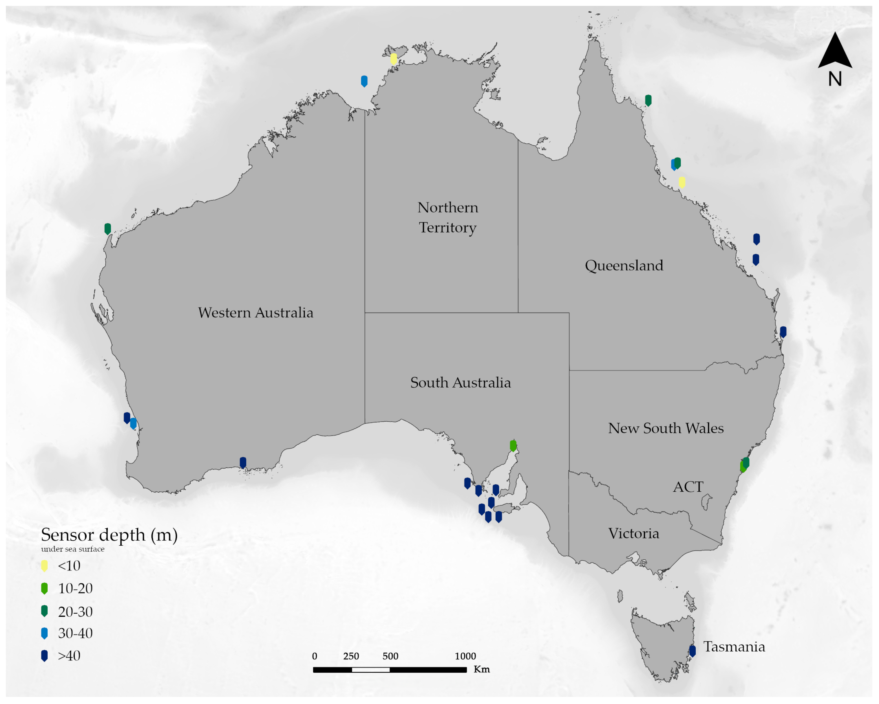
Appendix A. IMOS Sensors around Australia

Figure A1. Location and respective depths of IMOS sensors around Australia.
Remotesensing 16 02389 g0a1

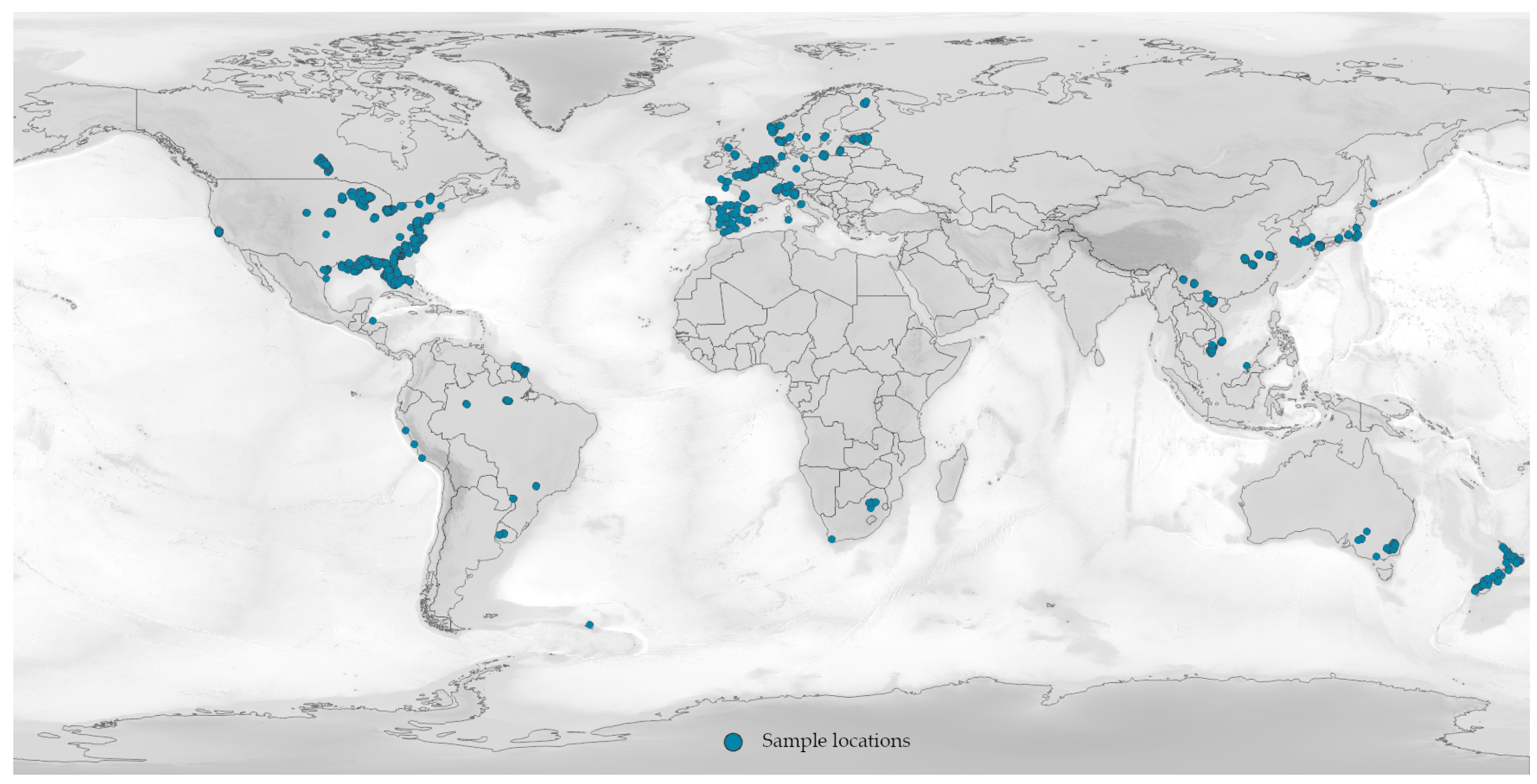
Appendix B. NOMAD Dataset Availability

Figure A2. NASA’s NOMAD dataset collected between 1991 till 2008 overlaid on the global map.
Remotesensing 16 02389 g0a2

Appendix C. GLORIA Dataset

Figure A3. Geographical location of GLORIA datasets (Dataset available at [83]).
Remotesensing 16 02389 g0a3

Appendix D. Bottom Depth

Table A1. Bottom depth (in meters) of surveyed locations.
St.HelensGreat Oyster Bay
Survey
Location ID
Location CoordinatesBottom
Depth (m)
Survey
Location ID
Location CoordinatesBottom
Depth (m)
2148.278421, −41.2933991.229148.219753, −42.1319279.3
3148.278547, −41.2915951.630148.214318, −42.1324489.6
4148.281969, −41.2896091.431148.209152, −42.1329739.7
5148.284655, −41.290452.832148.199544, −42.1231598.6
6148.287617, −41.2916115.733148.196921, −42.1226319
7148.28871, −41.2953257.534148.192777, −42.1221499.3
8148.286674, −41.2982969.535148.217547, −42.1173617.8
9148.288877, −41.30299316.236148.226515, −42.1103537.2
10148.298046, −41.3053815.137148.232691, −42.1040131.8
11148.298752, −41.3054324.2
12148.318981, −41.2941842
13148.319617, −41.2896261.9Bruny Island
14148.329573, −41.2775492.7
15148.331688, −41.276767449147.331163, −43.2030513
16148.313606, −41.3013623.750147.32499, −43.22212312
17148.278786, −41.32270610.951147.2903, −43.23978912.5
18148.274344, −41.3195460.652147.277944, −43.26233313.3
19148.279323, −41.3200892.553147.262045, −43.28464914.5
20148.286096, −41.3180314.554147.227832, −43.28221311.2
21148.283693, −41.315374155147.24639, −43.26881810.6
22148.285471, −41.31216818.756147.263409, −43.242085.8
23148.287293, −41.30914621.157147.357791, −43.12477313.9
24148.283931, −41.30785220.4
25148.279043, −41.3036365.1
26148.27892, −41.2989711.2

References

  1. Le, C.; Li, Y.; Zha, Y.; Sun, D.; Huang, C.; Lu, H. A four-band semi-analytical model for estimating chlorophyll a in highly turbid lakes: The case of Taihu Lake, China. Remote Sens. Environ. 2009, 113, 1175–1182. [Google Scholar]
  2. Gitelson, A.A.; Gurlin, D.; Moses, W.J.; Barrow, T. A bio-optical algorithm for the remote estimation of the chlorophyll a concentration in case 2 waters. Environ. Res. Lett. 2009, 4, 045003. [Google Scholar]
  3. Matthews, M.W. A current review of empirical procedures of remote sensing in inland and near-coastal transitional waters. Int. J. Remote Sens. 2011, 32, 6855–6899. [Google Scholar] [CrossRef]
  4. Koponen, S.; Attila, J.; Pulliainen, J.; Kallio, K.; Pyhälahti, T.; Lindfors, A.; Rasmus, K.; Hallikainen, M. A case study of airborne and satellite remote sensing of a spring bloom event in the Gulf of Finland. Cont. Shelf Res. 2007, 27, 228–244. [Google Scholar]
  5. Gordon, H.R. Diffuse reflectance of the ocean: The theory of its augmentation by chlorophyll a fluorescence at 685 nm. Appl. Opt. 1979, 18, 1161–1166. [Google Scholar] [PubMed]
  6. Yu, Y.; Chen, S.; Qin, W.; Lu, T.; Li, J.; Cao, Y. A Semi-Empirical Chlorophyll a Retrieval Algorithm Considering the Effects of Sun Glint, Bottom Reflectance, and Non-Algal Particles in the Optically Shallow Water Zones of Sanya Bay Using SPOT6 Data. Remote Sens. 2020, 12, 2765. [Google Scholar] [CrossRef]
  7. Matsushita, B.; Yang, W.; Chang, P.; Yang, F.; Fukushima, T. A simple method for distinguishing global Case-1 and Case-2 waters using SeaWiFS measurements. ISPRS J. Photogramm. Remote Sens. 2012, 69, 74–87. [Google Scholar]
  8. Morel, A.; Prieur, L. Analysis of variations in ocean color. Limnol. Oceanogr. 1977, 22, 709–722. [Google Scholar] [CrossRef]
  9. Sathyendranath, S. Remote Sensing of Ocean Colour in Coastal, and Other Optically-Complex, Waters; Report 3; International Ocean Colour Coordinating Group (IOCCG): Dartmouth, NS, Canada, 2000. [Google Scholar]
  10. Gholizadeh, M.H.; Melesse, A.M.; Reddi, L. A comprehensive review on water quality parameters estimation using remote sensing techniques. Sensors 2016, 16, 1298. [Google Scholar] [CrossRef]
  11. Ogashawara, I.; Kiel, C.; Jechow, A.; Kohnert, K.; Ruhtz, T.; Grossart, H.P.; Hölker, F.; Nejstgaard, J.C.; Berger, S.A.; Wollrab, S. The use of Sentinel-2 for chlorophyll a spatial dynamics assessment: A comparative study on different lakes in northern Germany. Remote Sens. 2021, 13, 1542. [Google Scholar] [CrossRef]
  12. Ansper, A.; Alikas, K. Retrieval of chlorophyll a from Sentinel-2 MSI data for the European Union water framework directive reporting purposes. Remote Sens. 2018, 11, 64. [Google Scholar] [CrossRef]
  13. Kuhn, C.; de Matos Valerio, A.; Ward, N.; Loken, L.; Sawakuchi, H.O.; Kampel, M.; Richey, J.; Stadler, P.; Crawford, J.; Striegl, R.; et al. Performance of Landsat-8 and Sentinel-2 surface reflectance products for river remote sensing retrievals of chlorophyll a and turbidity. Remote Sens. Environ. 2019, 224, 104–118. [Google Scholar] [CrossRef]
  14. Watanabe, F.; Alcantara, E.; Rodrigues, T.; Rotta, L.; Bernardo, N.; Imai, N. Remote sensing of the chlorophyll a based on OLI/Landsat-8 and MSI/Sentinel-2A (Barra Bonita reservoir, Brazil). An. Acad. Bras. Ciências 2017, 90, 1987–2000. [Google Scholar] [CrossRef] [PubMed]
  15. Lewis, M.D.; Jarreau, B.; Jolliff, J.; Ladner, S.; Lawson, T.A.; McCarthy, S.; Martinolich, P.; Montes, M. Assessing Planet Nanosatellite Sensors for Ocean Color Usage. Remote Sens. 2023, 15, 5359. [Google Scholar] [CrossRef]
  16. Yang, H.; Kong, J.; Hu, H.; Du, Y.; Gao, M.; Chen, F. A review of remote sensing for Water Quality Retrieval: Progress and challenges. Remote Sens. 2022, 14, 1770. [Google Scholar] [CrossRef]
  17. Greb, S.; Dekker, A.; Binding, C. (Eds.) Earth Observations in Support of Global Water Quality Monitoring; Number 17 in IOCCG Report Series; International Ocean Colour Coordinating Group: Dartmouth, NS, Canada, 2018. [Google Scholar]
  18. Bohn, V.Y.; Carmona, F.; Rivas, R.; Lagomarsino, L.; Diovisalvi, N.; Zagarese, H.E. Development of an empirical model for chlorophyll a and Secchi Disk Depth estimation for a Pampean shallow lake (Argentina). Egypt. J. Remote Sens. Space Sci. 2018, 21, 183–191. [Google Scholar] [CrossRef]
  19. Poddar, S.; Chacko, N.; Swain, D. Estimation of chlorophyll a in Northern Coastal Bay of Bengal using Landsat-8 OLI and Sentinel-2 MSI sensors. Front. Mar. Sci. 2019, 6, 598. [Google Scholar] [CrossRef]
  20. Song, K.; Wang, Z.; Blackwell, J.; Zhang, B.; Li, F.; Zhang, Y.; Jiang, G. Water quality monitoring using Landsat Themate Mapper data with empirical algorithms in Chagan Lake, China. J. Appl. Remote Sens. 2011, 5, 053506. [Google Scholar] [CrossRef]
  21. Härmä, P.; Vepsäläinen, J.; Hannonen, T.; Pyhälahti, T.; Kämäri, J.; Kallio, K.; Eloheimo, K.; Koponen, S. Detection of water quality using simulated satellite data and semi-empirical algorithms in Finland. Sci. Total Environ. 2001, 268, 107–121. [Google Scholar] [CrossRef]
  22. Dekker, A.G.; Vos, R.; Peters, S.W. Comparison of remote sensing data, model results and in situ data for total suspended matter (TSM) in the southern Frisian lakes. Sci. Total Environ. 2001, 268, 197–214. [Google Scholar] [CrossRef]
  23. Chang, K.W.; Shen, Y.; Chen, P.C. Predicting algal bloom in the Techi reservoir using Landsat TM data. Int. J. Remote Sens. 2004, 25, 3411–3422. [Google Scholar] [CrossRef]
  24. Kutser, T.; Pierson, D.C.; Kallio, K.Y.; Reinart, A.; Sobek, S. Mapping lake CDOM by satellite remote sensing. Remote Sens. Environ. 2005, 94, 535–540. [Google Scholar] [CrossRef]
  25. Mayo, M.; Gitelson, A.; Yacobi, Y.; Ben-Avraham, Z. Chlorophyll distribution in lake Kinneret determined from Landsat Thematic Mapper data. Remote Sens. 1995, 16, 175–182. [Google Scholar] [CrossRef]
  26. Tamiminia, H.; Salehi, B.; Mahdianpari, M.; Quackenbush, L.; Adeli, S.; Brisco, B. Google Earth Engine for geo-big data applications: A meta-analysis and systematic review. ISPRS J. Photogramm. Remote Sens. 2020, 164, 152–170. [Google Scholar] [CrossRef]
  27. Ma, Y.; Wu, H.; Wang, L.; Huang, B.; Ranjan, R.; Zomaya, A.; Jie, W. Remote sensing big data computing: Challenges and opportunities. Future Gener. Comput. Syst. 2015, 51, 47–60. [Google Scholar] [CrossRef]
  28. Acheampong, C. Deriving algal concentration from Sentinel-2 through a downscaling technique: A case near the intake of a desalination plant. J. Geophys. Res. 2018, 103, 24937–24953. [Google Scholar]
  29. Binding, C.; Greenberg, T.; Bukata, R. The MERIS Maximum Chlorophyll Index; its merits and limitations for inland water algal bloom monitoring. J. Great Lakes Res. 2013, 39, 100–107. [Google Scholar] [CrossRef]
  30. Chen, J.; Chen, S.; Fu, R.; Wang, C.; Li, D.; Peng, Y.; Wang, L.; Jiang, H.; Zheng, Q. Remote sensing estimation of chlorophyll A in case-II waters of coastal areas: Three-band model versus genetic algorithm–artificial neural networks model. IEEE J. Sel. Top. Appl. Earth Obs. Remote Sens. 2021, 14, 3640–3658. [Google Scholar] [CrossRef]
  31. Dekker, A.; Hestir, E. Evaluating the Feasibility of Systematic Inland Water Quality Monitoring with Satellite Remote Sensing; Commonwealth Scientific and Industrial Research Organization: Canberra, Australia, 2012. [Google Scholar]
  32. Gitelson, A.A.; Gurlin, D.; Moses, W.J.; Yacobi, Y.Z. Remote estimation of chlorophyll a concentration in inland, estuarine, and coastal waters. In Advances in Environmental Remote Sensing: Sensors, Algorithms, and Applications; Weng, Q., Ed.; Taylor & Francis Group: Boca Raton, FL, USA, 2011; Chapter 18. [Google Scholar]
  33. Kallio, K.; Koponen, S.; Pulliainen, J. Feasibility of airborne imaging spectrometry for lake monitoring—A case study of spatial chlorophyll a distribution in two meso-eutrophic lakes. Int. J. Remote Sens. 2003, 24, 3771–3790. [Google Scholar] [CrossRef]
  34. Kravitz, J.; Matthews, M.; Bernard, S.; Griffith, D. Application of Sentinel 3 OLCI for chl-a retrieval over small inland water targets: Successes and challenges. Remote Sens. Environ. 2020, 237, 111562. [Google Scholar] [CrossRef]
  35. Lins, R.C.; Martinez, J.M.; Motta Marques, D.D.; Cirilo, J.A.; Fragoso, C.R., Jr. Assessment of chlorophyll a remote sensing algorithms in a productive tropical estuarine-lagoon system. Remote Sens. 2017, 9, 516. [Google Scholar] [CrossRef]
  36. Malthus, T.J.; Lehmann, E.; Ho, X.; Botha, E.; Anstee, J. Implementation of a satellite based inland water algal bloom alerting system using analysis ready data. Remote Sens. 2019, 11, 2954. [Google Scholar] [CrossRef]
  37. Neil, C.; Spyrakos, E.; Hunter, P.D.; Tyler, A.N. A global approach for chlorophyll a retrieval across optically complex inland waters based on optical water types. Remote Sens. Environ. 2019, 229, 159–178. [Google Scholar] [CrossRef]
  38. O’Reilly, J.E.; Maritorena, S.; Mitchell, B.G.; Siegel, D.A.; Carder, K.L.; Garver, S.A.; Kahru, M.; McClain, C. Ocean color chlorophyll algorithms for SeaWiFS. J. Geophys. Res. Ocean. 1998, 103, 24937–24953. [Google Scholar] [CrossRef]
  39. Pahlevan, N.; Smith, B.; Schalles, J.; Binding, C.; Cao, Z.; Ma, R.; Alikas, K.; Kangro, K.; Gurlin, D.; Hà, N.; et al. Seamless retrievals of chlorophyll a from Sentinel-2 (MSI) and Sentinel-3 (OLCI) in inland and coastal waters: A machine-learning approach. Remote Sens. Environ. 2020, 240, 111604. [Google Scholar] [CrossRef]
  40. Gitelson, A. The peak near 700 nm on radiance spectra of algae and water: Relationships of its magnitude and position with chlorophyll concentration. Int. J. Remote Sens. 1992, 13, 3367–3373. [Google Scholar] [CrossRef]
  41. Gower, J.; Doerffer, R.; Borstad, G. Interpretation of the 685nm peak in water-leaving radiance spectra in terms of fluorescence, absorption and scattering, and its observation by MERIS. Int. J. Remote Sens. 1999, 20, 1771–1786. [Google Scholar] [CrossRef]
  42. Gilerson, A.A.; Gitelson, A.A.; Zhou, J.; Gurlin, D.; Moses, W.; Ioannou, I.; Ahmed, S.A. Algorithms for remote estimation of chlorophyll a in coastal and inland waters using red and near infrared bands. Opt. Express 2010, 18, 24109–24125. [Google Scholar] [CrossRef] [PubMed]
  43. Moses, W.J.; Gitelson, A.A.; Berdnikov, S.; Povazhnyy, V. Estimation of chlorophyll a concentration in case II waters using MODIS and MERIS data—successes and challenges. Environ. Res. Lett. 2009, 4, 045005. [Google Scholar] [CrossRef]
  44. Power, M.E.; Brozović, N.; Bode, C.; Zilberman, D. Spatially explicit tools for understanding and sustaining inland water ecosystems. Front. Ecol. Environ. 2005, 3, 47–55. [Google Scholar] [CrossRef]
  45. Moses, W.J.; Gitelson, A.A.; Berdnikov, S.; Saprygin, V.; Povazhnyi, V. Operational MERIS-based NIR-red algorithms for estimating chlorophyll a concentrations in coastal waters—The Azov Sea case study. Remote Sens. Environ. 2012, 121, 118–124. [Google Scholar] [CrossRef]
  46. Dogliotti, A.I.; Schloss, I.R.; Almandoz, G.O.; Gagliardini, D.A. Evaluation of SeaWiFS and MODIS chlorophyll a products in the Argentinean Patagonian continental shelf (38 S–55 S). Int. J. Remote Sens. 2009, 30, 251–273. [Google Scholar] [CrossRef]
  47. Hu, C.; Feng, L.; Lee, Z.; Franz, B.A.; Bailey, S.W.; Werdell, P.J.; Proctor, C.W. Improving satellite global chlorophyll a data products through algorithm refinement and data recovery. J. Geophys. Res. Ocean. 2019, 124, 1524–1543. [Google Scholar] [CrossRef]
  48. O’Reilly, J.E.; Werdell, P.J. Chlorophyll algorithms for ocean color sensors-OC4, OC5 & OC6. Remote Sens. Environ. 2019, 229, 32–47. [Google Scholar]
  49. Winarso, G.; Marini, Y. MODIS standard (OC3) chlorophyll a algorithm evaluation in Indonesian seas. Int. J. Remote Sens. Earth Sci. 2014, 11, 11–20. [Google Scholar] [CrossRef]
  50. Cherukuru, N.; Brando, V.E.; Schroeder, T.; Clementson, L.A.; Dekker, A.G. Influence of river discharge and ocean currents on coastal optical properties. Cont. Shelf Res. 2014, 84, 188–203. [Google Scholar] [CrossRef]
  51. Menken, K.D.; Brezonik, P.L.; Bauer, M.E. Influence of chlorophyll and colored dissolved organic matter (CDOM) on lake reflectance spectra: Implications for measuring lake properties by remote sensing. Lake Reserv. Manag. 2006, 22, 179–190. [Google Scholar] [CrossRef]
  52. Werdell, P.J.; Bailey, S.W. An improved in-situ bio-optical dataset for ocean color algorithm development and satellite data product validation. Remote Sens. Environ. 2005, 98, 122–140. [Google Scholar] [CrossRef]
  53. SeaBASS. NOMAD: NASA bio-Optical Marine Algorithm Dataset. 2012. Available online: https://seabass.gsfc.nasa.gov/wiki/NOMAD (accessed on 2 February 2023).
  54. Cloern, J.E. Our evolving conceptual model of the coastal eutrophication problem. Mar. Ecol. Prog. Ser. 2001, 210, 223–253. [Google Scholar] [CrossRef]
  55. Hu, C.; Lee, Z.; Franz, B. Chlorophyll aalgorithms for oligotrophic oceans: A novel approach based on three-band reflectance difference. J. Geophys. Res. Ocean. 2012, 117, C01011. [Google Scholar] [CrossRef]
  56. Schroeder, T.; Brando, V.; Cherukuru, N.; Clementson, L.; Blondeau-Patissier, D.; Dekker, A.; Schaale, M.; Fischer, J. Remote sensing of apparent and inherent optical properties of Tasmanian coastal waters: Application to MODIS data. In Proceedings of the XIX Ocean Optics Conference, Barga, Italy, 3–4 October 2008; pp. 6–10. [Google Scholar]
  57. Yacobi, Y.Z. From Tswett to identified flying objects: A concise history of chlorophyll a use for quantification of phytoplankton. Isr. J. Plant Sci. 2012, 60, 243–251. [Google Scholar] [CrossRef]
  58. Zhao, J.; Liu, D.; Zhu, Y.; Peng, H.; Xie, H. A review of forest carbon cycle models on spatiotemporal scales. J. Clean. Prod. 2022, 339, 130692. [Google Scholar] [CrossRef]
  59. Amani, M.; Ghorbanian, A.; Ahmadi, S.A.; Kakooei, M.; Moghimi, A.; Mirmazloumi, S.M.; Moghaddam, S.H.A.; Mahdavi, S.; Ghahremanloo, M.; Parsian, S.; et al. Google Earth engine cloud computing platform for remote sensing big data applications: A comprehensive review. IEEE J. Sel. Top. Appl. Earth Obs. Remote Sens. 2020, 13, 5326–5350. [Google Scholar] [CrossRef]
  60. Department of Natural Resources and Environment Tasmania. LIST Marine Leases; Department of Natural Resources and Environment Tasmania: Tasmania, Australia, 2022. Available online: https://maps.thelist.tas.gov.au/listmap/app/list/map (accessed on 2 September 2022).
  61. Tasmanian Government. Department of Natural Resources and Environment Tasmania: Aquaculture. Available online: https://nre.tas.gov.au/aquaculture/aquaculture-species-in-tasmania/salmon-farming (accessed on 20 May 2024).
  62. Oysters Tasmania—Our Industry. Available online: https://www.oysterstasmania.org/ourindustry.html (accessed on 8 May 2024).
  63. Department of Agriculture, Fisheries and Forestry. Aquaculture Industry in Australia; 2020. Available online: https://www.agriculture.gov.au/agriculture-land/fisheries/aquaculture/aquaculture-industry-in-australia (accessed on 2 September 2022).
  64. Franz, B.A.; Bailey, S.W.; Kuring, N.; Werdell, P.J. Ocean color measurements with the Operational Land Imager on Landsat-8: Implementation and evaluation in SeaDAS. J. Appl. Remote Sens. 2015, 9, 096070. [Google Scholar] [CrossRef]
  65. Nazeer, M.; Bilal, M.; Nichol, J.E.; Wu, W.; Alsahli, M.M.; Shahzad, M.I.; Gayen, B.K. First experiences with the Landsat-8 aquatic reflectance product: Evaluation of the regional and ocean color algorithms in a coastal environment. Remote Sens. 2020, 12, 1938. [Google Scholar] [CrossRef]
  66. Wu, Q. geemap: A Python package for interactive mapping with Google Earth Engine. J. Open Source Softw. 2020, 5, 2305. [Google Scholar] [CrossRef]
  67. Cardille, J.A.; Crowley, M.A.; Saah, D.; Clinton, N.E. Cloud-Based Remote Sensing with Google Earth Engine: Fundamentals and Applications; Springer Nature Switzerland AG: Cham, Switzerland, 2023. [Google Scholar]
  68. Engine, G.E. LANDSAT/LC08/C02/T1_L2—Landsat 8 Collection 2, Tier 1, Level-2 Surface Reflectance. Available online: https://developers.Google.com/earth-engine/datasets/catalog/LANDSAT_LC08_C02_T1_L2 (accessed on 4 April 2022).
  69. Dekker, A.G.; Phinn, S.R.; Anstee, J.; Bissett, P.; Brando, V.E.; Casey, B.; Fearns, P.; Hedley, J.; Klonowski, W.; Lee, Z.P.; et al. Intercomparison of shallow water bathymetry, hydro-optics, and benthos mapping techniques in Australian and Caribbean coastal environments. Limnol. Oceanogr. Methods 2011, 9, 396–425. [Google Scholar] [CrossRef]
  70. Cherukuru, N.; Ford, P.W.; Matear, R.J.; Oubelkheir, K.; Clementson, L.A.; Suber, K.; Steven, A.D. Estimating dissolved organic carbon concentration in turbid coastal waters using optical remote sensing observations. Int. J. Appl. Earth Obs. Geoinf. 2016, 52, 149–154. [Google Scholar] [CrossRef]
  71. Kirk, J.T. Light and Photosynthesis in Aquatic Ecosystems; Cambridge University Press: Cambridge, UK, 1994. [Google Scholar]
  72. Weeks, S.; Werdell, P.J.; Schaffelke, B.; Canto, M.; Lee, Z.; Wilding, J.G.; Feldman, G.C. Satellite-derived photic depth on the Great Barrier Reef: Spatio-temporal patterns of water clarity. Remote Sens. 2012, 4, 3781–3795. [Google Scholar] [CrossRef]
  73. Tasmanian Tide Tables. Bureau of Meteorology, Australian Government. 2024. Available online: http://www.bom.gov.au/oceanography/projects/ntc/tas_tide_tables.shtml (accessed on 12 May 2024).
  74. Olmanson, L.G.; Brezonik, P.L.; Finlay, J.C.; Bauer, M.E. Comparison of Landsat 8 and Landsat 7 for regional measurements of CDOM and water clarity in lakes. Remote Sens. Environ. 2016, 185, 119–128. [Google Scholar] [CrossRef]
  75. Cui, T.; Zhang, J.; Wang, K.; Wei, J.; Mu, B.; Ma, Y.; Zhu, J.; Liu, R.; Chen, X. Remote sensing of chlorophyll a concentration in turbid coastal waters based on a global optical water classification system. ISPRS J. Photogramm. Remote Sens. 2020, 163, 187–201. [Google Scholar] [CrossRef]
  76. IMOS. AODN Open Access to Ocean Data. 2021. Available online: https://portal.aodn.org.au/search?uuid=8964658c-6ee1-4015-9bae-2937dfcc6ab9https://portal.aodn.org.au/search (accessed on 9 April 2022).
  77. Gordon, H.R.; McCluney, W. Estimation of the depth of sunlight penetration in the sea for remote sensing. Appl. Opt. 1975, 14, 413–416. [Google Scholar] [CrossRef] [PubMed]
  78. Lehmann, M.K.; Gurlin, D.; Pahlevan, N.; Alikas, K.; Anstee, J.; Balasubramanian, S.V.; Barbosa, C.C.; Binding, C.; Bracher, A.; Bresciani, M.; et al. GLORIA-A globally representative hyperspectral in situ dataset for optical sensing of water quality. Sci. Data 2023, 10, 100. [Google Scholar] [CrossRef] [PubMed]
  79. Pyo, J.; Duan, H.; Baek, S.; Kim, M.S.; Jeon, T.; Kwon, Y.S.; Lee, H.; Cho, K.H. A convolutional neural network regression for quantifying cyanobacteria using hyperspectral imagery. Remote Sens. Environ. 2019, 233, 111350. [Google Scholar] [CrossRef]
  80. Mishra, S.; Mishra, D.R. Normalized difference chlorophyll index: A novel model for remote estimation of chlorophyll a concentration in turbid productive waters. Remote Sens. Environ. 2012, 117, 394–406. [Google Scholar] [CrossRef]
  81. Gitelson, A.A.; Dall’Olmo, G.; Moses, W.; Rundquist, D.C.; Barrow, T.; Fisher, T.R.; Gurlin, D.; Holz, J. A simple semi-analytical model for remote estimation of chlorophyll a in turbid waters: Validation. Remote Sens. Environ. 2008, 112, 3582–3593. [Google Scholar] [CrossRef]
  82. Bright, C.; Ardila, D.; Hestir, E.; Malthus, T.; Matthews, M.; Thompson, D.; Carter, N.; Dekker, A.; Frasson, R.; Green, R.; et al. The AquaSat-1 Mission Concept: Actionable Information on Water Quality and Aquatic Ecosystems for Australia and Western USA. In Proceedings of the IGARSS 2023—2023 IEEE International Geoscience and Remote Sensing Symposium, Pasadena, CA, USA, 16–21 July 2023; IEEE: Piscataway, NJ, USA, 2023; pp. 4590–4593. [Google Scholar]
  83. Lehmann, M.K.; Gurlin, D.; Pahlevan, N.; Alikas, K.; Anstee, J.M.; Balasubramanian, S.V.; Barbosa, C.C.F.; Binding, C.; Bracher, A.; Bresciani, M.; et al. GLORIA—A global dataset of remote sensing reflectance and water quality from inland and coastal waters. Sci. Data 2022, 10, 100. [Google Scholar] [CrossRef]
Figure 1. Type of water based on the inherent properties, adopted from IOCCG [9].
Remotesensing 16 02389 g001
Figure 2. Survey locations of Tasmanian east coast. From north to south: (a) St.Helens, (b) Great Oyster Bay and (c) Bruny Island, Great Bay. Each numbered dot represents a location visited in September 2022, where field sampling was conducted to measure surface chlorophyll. The highlighted sites in green, labelled 10, 34 and 54, are presented in a detailed time-series analysis in Figure 8. The source of aquaculture site locations in Tasmania is provided by [60].
Remotesensing 16 02389 g002
Figure 3. Outline of processing steps used to (a) extract data from satellite images at field study sites to link with in situ data; (b) develop models to estimate Chlorophyll a concentration from satellite reflectance and field measurements; (c) produce time-series of output Chlorophyll a map at each study site; and (d) validate estimated Chlorophyll levels against field data not used in model development.
Remotesensing 16 02389 g003
Figure 4. Surface reflectance corrected false colour composite ARD data with cloud mask for each of the study sites from Figure 2. Survey locations at site (a) St. Helens, site (b) Great Oyster Bay and site (c) Bruny island. Base map source: DPIPWE, ESRI, HERE, Garmin, Foursquare, METI/NASA, USGS.
Remotesensing 16 02389 g004
Figure 5. Scatter plots of extracted chlorophyll a and modelled Chl-a vs in situ data at different locations in mg/m3. The top row of figures (ac) initially calculated Chl-a values without any parameter adjustments, the lower row of figures (df) modelled surface (site-specific coefficient applied) and in situ data on the x-axis.
Remotesensing 16 02389 g005
Figure 6. Modelled Chl-a concentration in mg/m3. Survey locations at site (a) St. Helens, site (b) Great Oyster Bay and site (c) Bruny Island. Base map source: Earthstar Geographics.
Remotesensing 16 02389 g006
Figure 7. Validation of temporal variation plot. The solid line represents the linear regression line based on all data, while the grey dotted lines depict the potential linear least squares fit excluding the outlier points. The red circles indicate possible outliers in the data.
Remotesensing 16 02389 g007
Figure 8. Time-series graph of surface chlorophyll a estimates between 2019 and 2023, using the automated GEE model. Each point symbolises a pixel value extracted at a field survey location (Figure 2) at site 10 for St. Helens (a), site 34 for Great Oyster Bay (b) and site 54 for Bruny Island (c).
Remotesensing 16 02389 g008
Table 1. Landsat 8 surface reflectance product for Chl-a extraction.
SensorMap
Label
LocationSurvey
Date
Image Capture DateImage
Landsat 8aSTH13-SEP-2211-SEP-22LANDSAT/LC08/C02/T1_L2/LC08_089089_20220911
bGOB15-SEP-2218-SEP-22LANDSAT/LC08/C02/T1_L2/LC08_089089_20220918
cBNI16-SEP-2218-SEP-22LANDSAT/LC08/C02/T1_L2/LC08_089090_20220918
Table 2. In situ stationary sensor-deployment details.
SensorLocationLocationInstallation Date
Multi-parameter147.363586, −43.207112BNI21 October
Xylem Exo 2148.210739, −42.131580GOB23 May
Table 3. Chl-a fourth-order polynomial model based on band ratios on water surface reflectance with r 2 values.
LocationSitesn r 2 RMSE (mg/m3)Remarks
STHAll depths *250.39 uncorrected **
Depth 2.0 m *190.59 uncorrected
0.750.74modelled **
GOBAll depths80.41 uncorrected
0.990.22modelled
BNIAll depths60.33 uncorrected
0.930.14modelled
CombinedDepth 2.0 m330.10 uncorrected
0.10 modelled
* All indicates inclusion of all collected samples; Depth2 m indicates exclusion of sites with water column depth less than 2 m. ** the modelled data are calibrated using the in situ data, while the uncorrected data are the direct output of the empirical blue-green model.
Table 4. Data availability.
DatasetAvailabilityDepthAustralian Waters
Coastal
Waters
Inland
Waters
NOMAD1991–2008unknownXX
IMOS2008–to date12–500 mX
GLORIAtill 20220–500 mX
Disclaimer/Publisher’s Note: The statements, opinions and data contained in all publications are solely those of the individual author(s) and contributor(s) and not of MDPI and/or the editor(s). MDPI and/or the editor(s) disclaim responsibility for any injury to people or property resulting from any ideas, methods, instructions or products referred to in the content.

