Abstract
Sea surface target detection is a key stage in a typical target detection system and directly influences the performance of the whole system. As an effective discriminator, the one-class support vector machine (OCSVM) has been widely used in target detection. In OCSCM, training samples are first mapped to the hypersphere in the kernel space with the Gaussian kernel function, and then, a linear classification hyperplane is constructed in each cluster to separate target samples from other classes of samples. However, when the distribution of the original data is complex, the transformed data in the kernel space may be nonlinearly separable. In this situation, OCSVM cannot classify the data correctly, because only a linear hyperplane is constructed in the kernel space. To solve this problem, a novel one-class classification algorithm, referred to as ensemble one-class support vector machine (En-OCSVM), is proposed in this paper. En-OCSVM is a hybrid model based on -means clustering and OCSVM. In En-OCSVM, training samples are clustered in the kernel space with the -means clustering algorithm, while a linear decision hyperplane is constructed in each cluster. With the combination of multiple linear classification hyperplanes, a complex nonlinear classification boundary can be achieved in the kernel space. Moreover, the joint optimization of the -means clustering model and OCSVM model is realized in the proposed method, which ensures the linear separability of each cluster. The experimental results based on the synthetic dataset, benchmark datasets, IPIX datasets, and SAR real data demonstrate the better performance of our method over other related methods.
1. Introduction and Background
In the conventional two-classification problem, two classes of samples are available in the training dataset, and the classification boundary is learned based on both classes of data, such as the support vector machine [1]. However, it is sometimes expensive or difficult to obtain both classes of data in practice. Therefore, only one class of data are available in the training stage, which is referred to as a one-class classification (OCC) problem. One-class classification is a task that identifies one class of samples (target samples) from another class of samples using only the target class of training samples. In some cases, one-class classification is also known as novelty detection, anomaly detection, or fault detection. Many real-world applications can be regarded as one-class classification problems, such as regional urban extent extraction [2], US urban extent mapping from MODIS data [3], supervised segment generation of geographic samples [4], Invasive Plant Spartina alterniflora detection [5], and Urban Built-Up Area Extraction [6].
To solve the OCC problem, a variety of one-class classifiers have been proposed over the past years [3,7,8,9,10,11,12,13,14]. In general, these one-class classification methods can be grouped into five categories [15]: (1) probabilistically based methods; (2) distance-based methods; (3) reconstruction-based methods; (4) domain-based methods; and (5) theoretic information-based methods. Probabilistically based methods try to estimate the generative probability density function (PDF) of the target samples based on the training dataset. Based on the PDF, a threshold is set to define the decision boundary, and a test sample comes from the same distribution if the value of the test sample is larger than the threshold. Typical examples of probabilistically based methods include Gaussian distribution, Gaussian mixture models (GMMs) [16,17], and Student’s t distribution [18]. Distance-based methods include clustering-based and near-neighbor-based methods, and the key to such methods is to define suitable distance metrics to compute the similarity measure. The well-known distance-based methods use -means clustering [19] and the -near neighbors [20] algorithm. Reconstruction-based methods, such as Principal Component Analysis (PCA) [21] and neural network [19], can autonomously model the underlying samples, and the reconstruction error is used to determine whether a test data point is an outlier or not. Domain-based methods create a decision boundary based on the structure of the training samples. Well-known examples are support vector data description (SVDD) [22] and one-class support vector machine (OCSVM) [23]. Theoretic information-based methods compute the entropy or relative entropy of the samples, and the outlier significantly alters the entropy or relative entropy of the otherwise normal samples.
In the above one-class classifiers, OCSVM is a widely used classifier because of its good generalization ability. In OCSCM, training samples are mapped to the hypersphere in the kernel space with the Gaussian kernel function first, and then, a linear classification hyperplane is constructed to separate target samples from other classes of samples. However, although OCSVM has achieved success in many applications, there is one drawback for OCSVM, i.e., OCSVM cannot classify data correctly when the distribution of data is complex. To solve this problem, Cyganek et al. [24] present an extension of the OCSVM into an ensemble of soft OCSVM classifiers, which can achieve a complex nonlinear decision boundary through the joining of several OCSVMs. Inspired by this idea, a novel one-class classifier, referred to as ensemble one-class support vector machine (referred to as En-OCSVM), is proposed in this paper. Our method is a mixture model of -means clustering and OCSVM models. In the proposed method, the training samples are clustered in the kernel space with -means clustering, while a linear classification boundary is constructed in each cluster. Through the mixture of multiple linear decision boundaries, complex nonlinear decision boundaries can be achieved in the kernel space.
The main contributions of this paper are summarized as follows:
- A mixture model based on the -means clustering algorithm and OCSVM for one-class classification is proposed.
- Through the mixture of multiple linear decision boundaries, complex nonlinear decision boundaries can be achieved in the kernel space, which can enhance the performance of the OCSVM, especially when the distribution of data is complex.
- The joint optimization of the -means clustering model and OCSVM model is realized based on support vectors (SVs), which ensures the linear separability of each cluster.
2. One-Class Support Vector Machine
OCSVM is a max-margin classifier inspired by two-class SVM. In OCSVM, a classification hyperplane is constructed in the kernel space with two criteria: (1) most of the target samples are located at the upper end of the hyperplane; (2) the distance between the origin and the hyperplane is maximum. The optimization function of OCSVM is shown in Equation (1):
where is the slope of the hyperplane, is the intercept of the hyperplane, is the projection of in the feature space with the kernel function, is a slack variable, and the constant gives an upper bound on the fraction of outliers.
The dual optimization problem of Equation (1) can be obtained with Lagrangian multipliers:
where is the kernel function. Samples with parameter greater than 0 are support vectors. The optimization function of Equation (2) can be solved with the sequential minimal optimization (SMO) algorithm [25]. The slope and intercept of OCSVM are given as follows:
In OCSVM, most of the coefficients are 0, and samples with coefficients greater than 0 are support vectors (SVs). We can see from Equation (3) that the slope and intercept of OCSVM are determined via SVs. Therefore, the decision boundary is defined based on SVs.
In most applications using OCSVM, Gaussian kernel function is the most used kernel function [26,27,28,29,30]. Moreover, experiments conducted by Alashwal et al. [31] showed that the Gaussian kernel function gives the best performance compared to other types of kernel functions. Therefore, the Gaussian kernel function is used in conjunction with OCSVM in the paper.
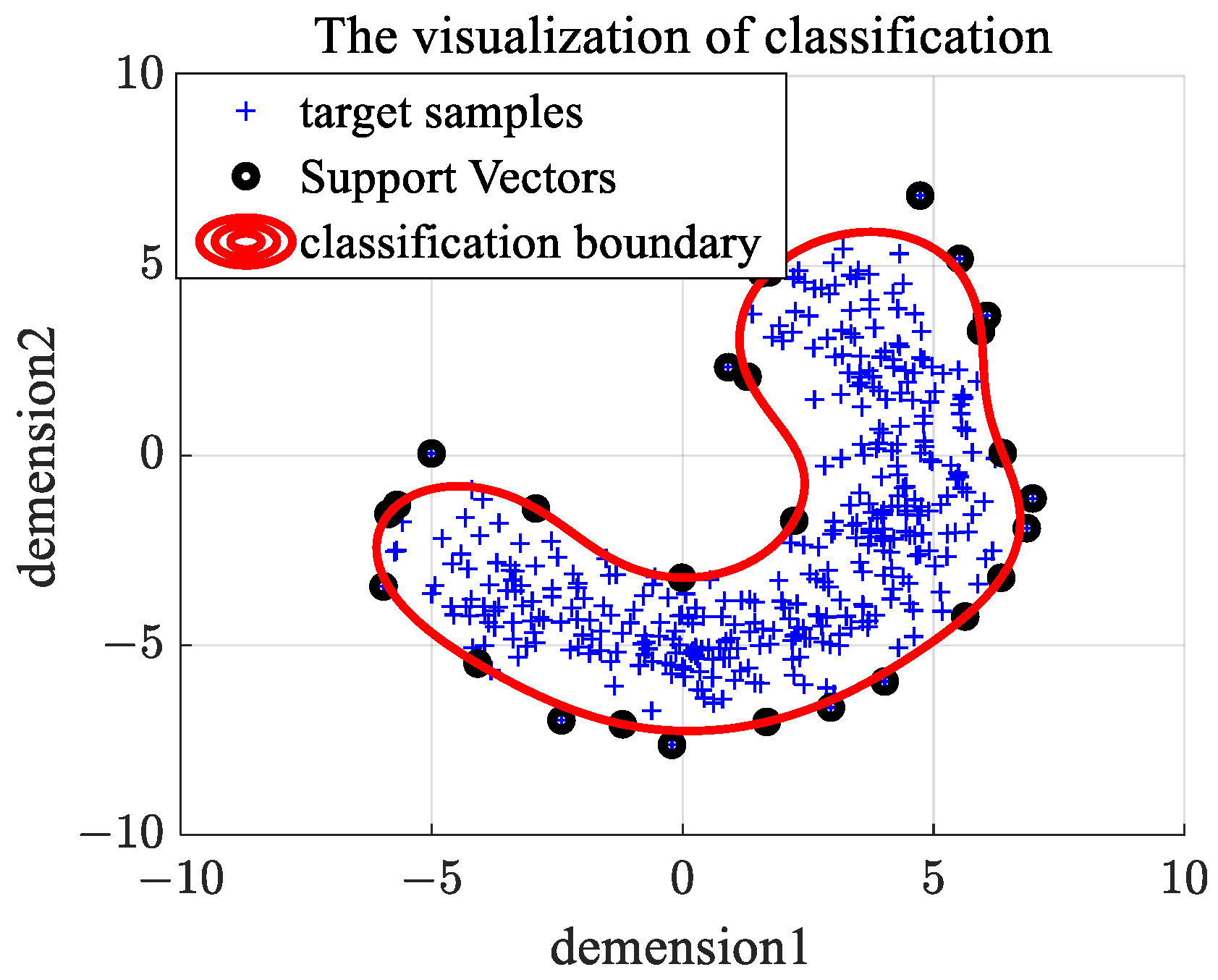
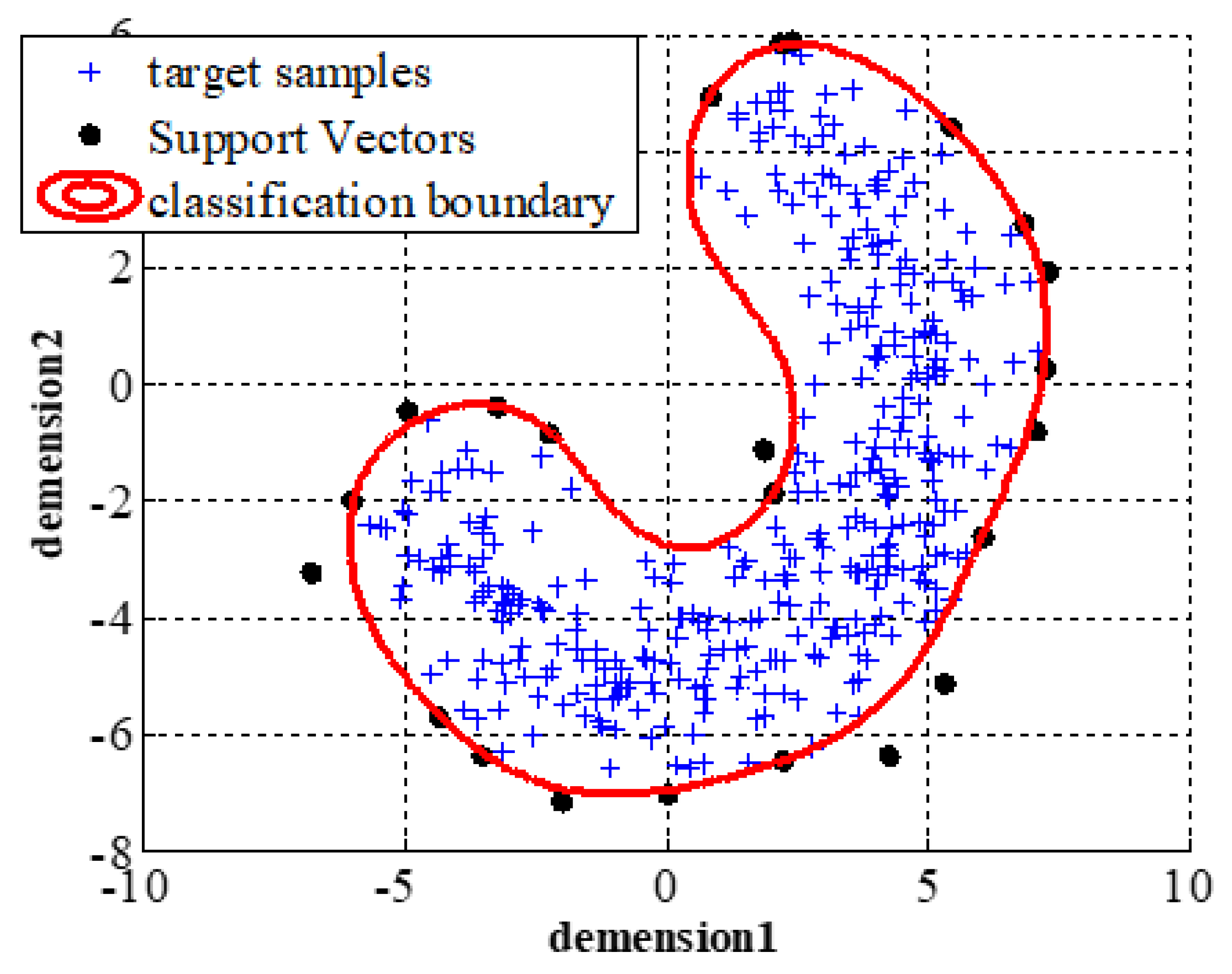
An example of the classification boundary for OCSVM is given in Figure 1. We generate banana-shaped synthetic data as target samples, and the SVs and classification boundary are shown in Figure 1. We can see from Figure 1 that SVs are the edge samples (located in the edge region of shape distribution) and can represent the shape distribution of target data, which is the core of joint optimization of the k-means clustering model and OCSVM model.
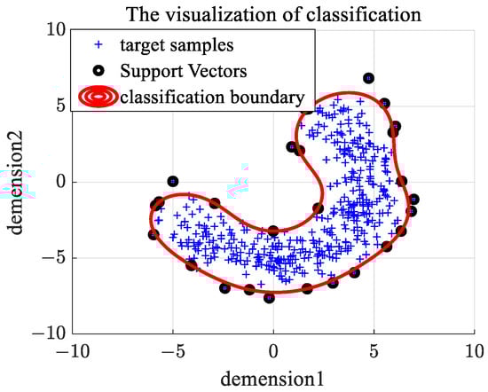
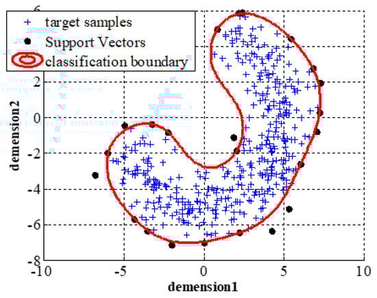
Figure 1.
Decision boundary of OCSVM on banana-shaped data.
3. Ensemble One-Class Support Vector Machine
In this section, we introduce the proposed method, e.g., En-OCSVM. In Section 3.1, we first describe the -means clustering in the kernel space. Then, the En-OCSVM model is given in Section 3.2. Finally, the prediction procedure of En-OCSVM is shown in Section 3.3.
3.1. k-Means Clustering in the Kernel Space
The -means clustering algorithm finds partitions in the kernel space based on minimizing the within-cluster sum-of-squares:
where is the projection of the input data , is the number of clusters, is the mean vector of the cluster, is the index set of the cluster, and is the number of samples belonging to the cluster.
The Gaussian kernel function is the inner product of two transformed samples:, where is the Gaussian kernel parameter. Using the Gaussian kernel function, Equation (4) can be rewritten as Equation (5):
In OCSVM, if the model parameter , the sample is the support vector. The support vectors describe the boundaries of data distribution. Therefore, the mean in k-means clustering can be represented with support vectors belonging to the cluster:
where represents the support vector belonging to the cluster, is index set of the support vector belonging to the cluster, and is the number of support vectors belonging to the cluster.
Based on Equations (5) and (6), the optimization problem of -means clustering in the kernel space can be rewritten as Equation (7):
The iterative optimization solution based on a greedy algorithm is used to solve the problem of Equation (7). The parameter optimization procedure of -means clustering in the kernel space based on SVs is given in Algorithm 1.
| Algorithm 1: The parameter optimization procedure of -means clustering |
| Input: input dataset , the number of clusters , the support vector set , and the Gaussian kernel parameter . |
| Randomly initialize the cluster partition of the input data, and obtain the cluster partition of the support vectors via ; |
| Flag = true; |
| While Flag |
| Update the clustering index corresponding to the sample via |
| Collect the clustering index to update the cluster partition and |
| If == |
| Flag = False; |
| Else |
| =; |
| End If |
| End While |
| Output: The cluster partition |
3.2. The Formulation of Ensemble OCSVM
In En-OCSVM, the samples are first transformed to the kernel space with a Gaussian kernel function. Then, the -means clustering algorithm is used to cluster the transformed samples in the kernel space. Meanwhile, a linear decision hyperplane is constructed in each cluster via OCSVM. The -means clustering and OCSVMs are jointly optimized through support vectors. Specifically, the clustering parameters optimization of -means clustering requires the support vectors determined by OCSVM, and the parameters’ optimization of OCSVM in each cluster requires the clustering labels determined by -means clustering. The joint optimization of the -means clustering and OCSVMs guarantees the consistency of clustering and linear separability in each cluster.
Based on Equations (2) and (7), the optimization problem of En-OCSVM can be represented as Equation (8).
where is the slope of the hyperplane in the th cluster, is the intercept of the hyperplane in the th cluster, and is the number of samples in the th cluster.
The optimization function of Equation (8) can be solved via the iteration optimization technique. Firstly, fix the parameters of each OCSVM and update the parameters of -means clustering algorithm. When the clustering index of samples is obtained, the optimization problem of OCSVMs can be solved based on the SMO algorithm. Parameters in both the -means clustering and OCSVM are updated iteratively until the clustering index no longer changes. The parameter optimization procedure of En-OCSVM is given in Algorithm 2.
In En-OCSVM, through the mixture of multiple linear decision boundaries, a complex nonlinear decision boundary can be achieved in the kernel space, which can enhance the performance of OCSVM, especially when the distribution of data is complex. The 2D illustrations of the classification hyperplanes for En-OCSVM and OCSVM are given in Figure 2a,b. We can see that some misclassified samples in the OCSVM are rejected in the En-OCSVM.
| Algorithm 2: The parameter optimization procedure of En-OCSVM |
| Input: input dataset , the number of clusters , and the Gaussian kernel parameter σ. |
|
| Output: The cluster partition , the model parameters , the support vector set . |
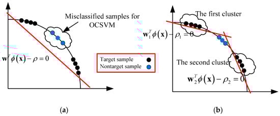
Figure 2.
The 2D illustrations of the classification hyperplane for En-OCSVM and OCSVM. (a) OCSVM; (b) En-OCSVM.
3.3. The Prediction Procedure of En-OCSVM
When a test sample is given, the cluster index of the sample is first obtained based on Equation (9):
Then, the classification label is given based on Equation (10):
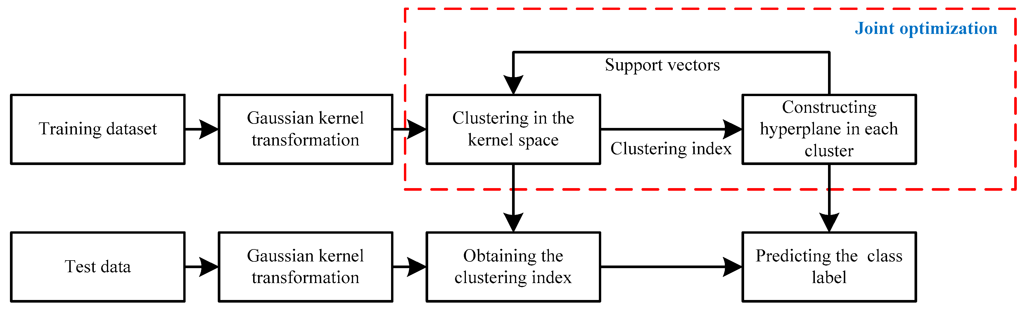
The flow chart of En-OCSVM is shown in Figure 3.
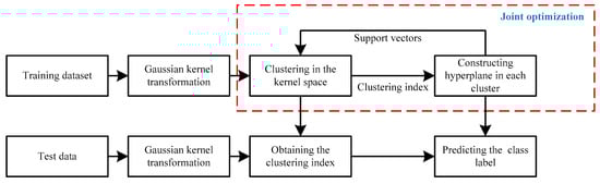
Figure 3.
The flow chart of En-OCSVM.
4. Experimental Results
In this section, the performance of our method is evaluated on synthetic datasets, benchmark datasets, sea surface datasets and SAR real data. Based on synthetic datasets, the clustering results and decision boundaries of En-OCSVM are visualized to demonstrate the qualitative effectiveness of our method. The quantitative comparisons between our method and other one-class classifiers are conducted based on benchmark datasets, sea surface datasets and SAR real data.
4.1. Dataset Description
In the experiments, five benchmark datasets, Glass, Parkinson, Spice, Pendigits and Waveform datasets from the repository of the University of California (https://archive.ics.uci.edu/dataset/ accessed on 19 May 2021), were used.
The Glass dataset belongs to Physics and Chemistry, and the study of the classification of types of glass was motivated by criminological investigation. The Parkinson dataset is composed of a range of biomedical voice measurements from 31 people, 23 with Parkinson’s disease (PD). The main aim of the data is to discriminate healthy people from those with PD. Splice dataset points on a DNA sequence at which ‘superfluous’ DNA is removed during the process of protein creation in higher organisms. The Pendigits dataset is a digit database comprising 250 samples from 44 writers. The samples written by 30 writers are used for training, cross-validation and writer-dependent testing, and the digits written by the other 14 are used for writer-independent testing. The Waveform dataset includes three classes, each generated from a combination of 2 of 3 “base” waves. The division of the training and testing sets in the experiment is shown in Table 1.

Table 1.
The description of the benchmark datasets.
IPIX datasets (http://soma.mcmaster.ca/ipix/dartmouth/datasets.html accessed on 1 January 2017) are widely used in target detection under sea clutter and are collected by the IPIX radar at the staring mode in 1993 for four polarizations (HH, VV, HV, and VH polarization) with a pulse repetition frequency of 1000 Hz. The IPIX radar is an instrumentation-quality, coherent, and dual-polarized X-band (9.39 GHz) radar system. In IPIX datasets, the target is a small spherical block of Styrofoam wrapped with wire mesh, and the average target-to-clutter ratio varies in the range of 0–6 dB. The range resolution is 30 m, and each dataset consists of a time series of length at 14 contiguous range cells. In the experiments, we choose two datasets from IPIX datasets, and a detailed description of these two datasets is shown in Table 2.
Table 2.
Description of experimental IPIX datasets.
For each echo cell, we use the windowing technique with a fixed time window of 1.024 s to extract 5-dimensional features in each time window through Cloude polarization decomposition [32] and Krogager polarization decomposition [33]. After the above data preprocessing, we obtain 1280 clutter samples and 128 target samples for each dataset.
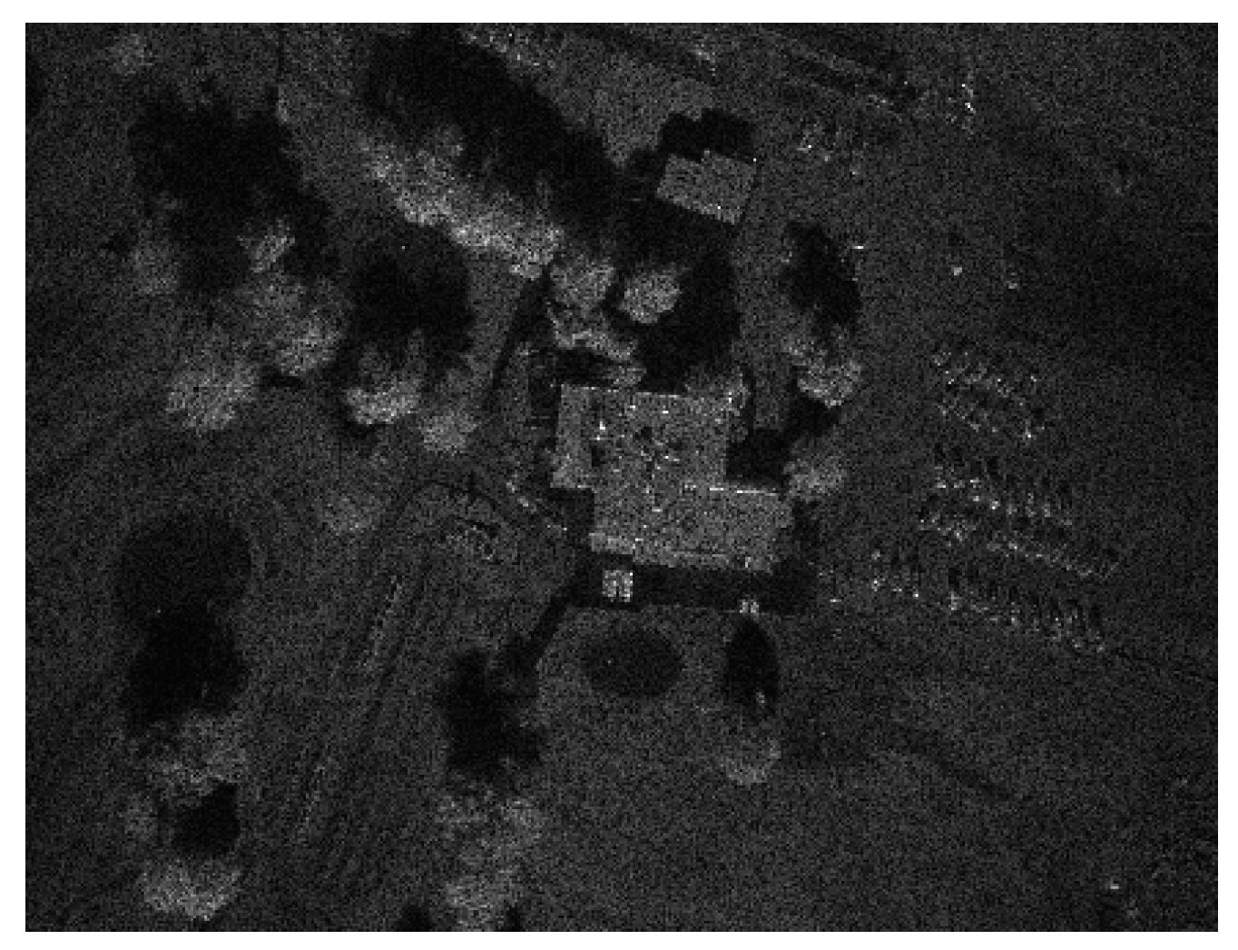
The SAR real data come from the Sandia MiniSAR dataset (http://www.sandia.gov/radar/imagery accessed on 1 December 2020). There are nine total SAR images in this dataset, in which the target sample is a car, while the clutter samples include building clutter, road edges, trees, and grasslands. We choose three images as the training SAR images and one image as the test SAR images. The training and test images are shown in Figure 4 and Figure 5. We can see from Figure 4 and Figure 5 that the clutter in the training set is mainly road edge, while the types of clutter in the test set include buildings, trees, grasslands, etc.
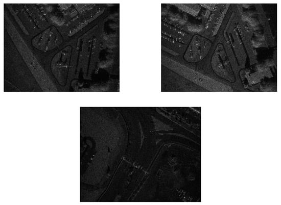
Figure 4.
The training SAR images used in the experiment.
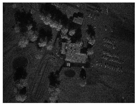
Figure 5.
The test SAR images used in the experiment.
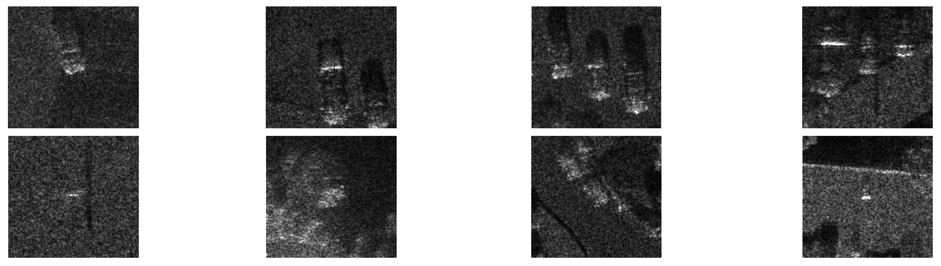
With the constant false alarm rate (CFAR) detection algorithm, we obtained 346 patches, including 248 target patches and 98 non-target patches, from SAR images in the Sandia MiniSAR dataset, and some patch examples are shown in Figure 6. We set the patches only including the car as target samples and the remaining patches as clutter samples. In Figure 6, the first row corresponds to target samples, and the second row corresponds to clutter samples.
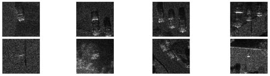
Figure 6.
Some patch examples from SAR images in Sandia MiniSAR dataset, where the first row corresponds to the target samples, and the second row corresponds to the clutter samples.
All methods were implemented in MATLAB software, 2019 version. For OCSVM, WOC-SVM and En-OCSVM, a modified LIBSVM library was employed (original version provided by Chang et al. [34]). Experiments were run on a computer with 16GB RAM, Gen Intel(R) Core(TM) i7-1260P 2.10 GHz. Readers interested in our method can obtain relevant code and datasets through email (scchen0115@njtech.edu.cn).
4.2. Visual Results on Synthetic Dataset
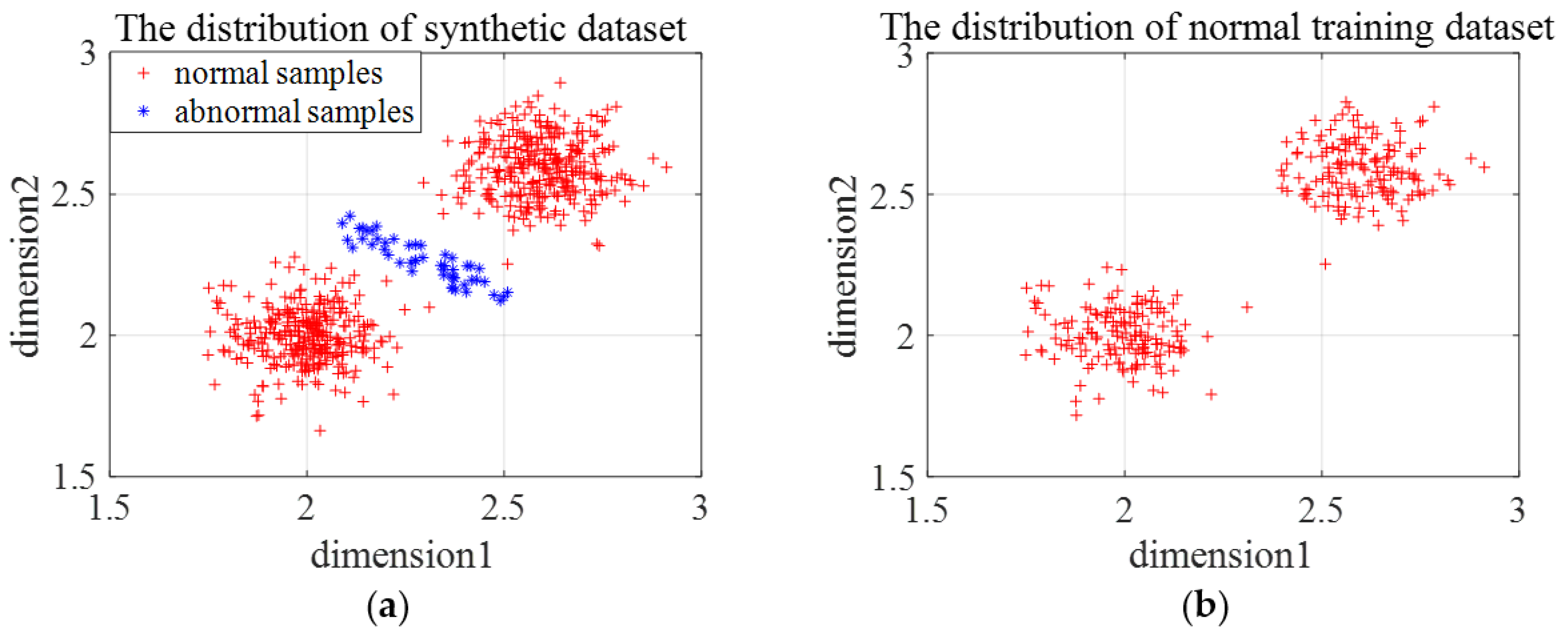
Three types of synthetic datasets are generated to evaluate the effectiveness and the limitations of En-OCSVM. The distribution of the first type of synthetic data is shown in Figure 7a. We choose one class of samples as normal samples, and the distribution of training samples is shown in Figure 7b. The number of clusters in -means clustering is set as 2, and the rejection rate of training samples in OCSVM is set as 0.1. Figure 8a gives the clustering results of En-OCSVM, and the classification boundary of En-OCSVM is shown in Figure 8b. It can be seen from Figure 8a,b that the training samples were correctly clustered into two clusters, and the classification boundary in each cluster can correctly distinguish between normal samples and abnormal samples.
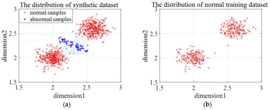
Figure 7.
The distribution of the first type of synthetic data and training samples. (a) The distribution of the first type of synthetic data; (b) the distribution of the training samples.

Figure 8.
The clustering result and classification boundary for the first type of synthetic dataset. (a) The initial clustering result; (b) the classification boundary.
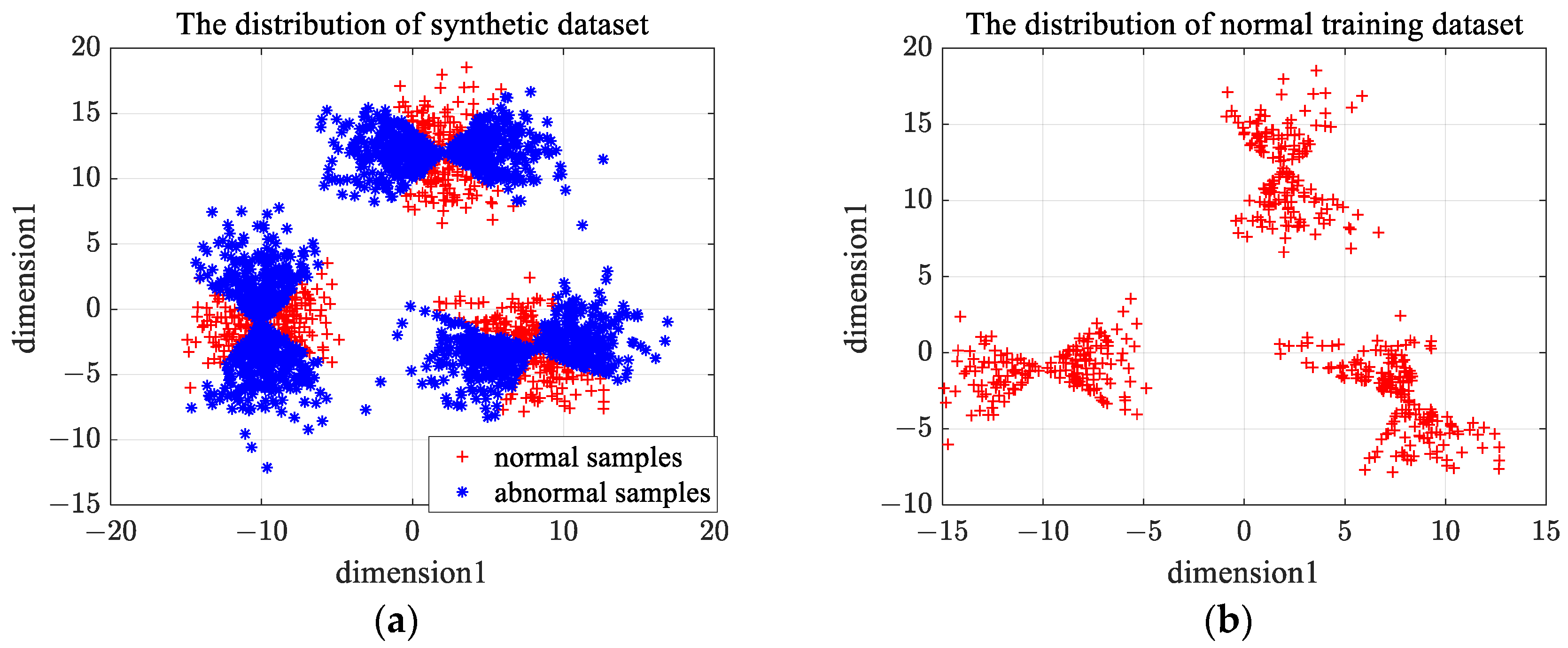
The distribution of the second type of synthetic data is shown in Figure 9a. We choose one class of samples as normal samples, and the distribution of training samples is shown in Figure 9b. The number of clusters in -means clustering is set as 6, and the rejection rate of training samples in OCSVM is set as 0.1. Figure 10a gives the clustering results of En-OCSVM, and the classification boundary of En-OCSVM is shown in Figure 10b. It can be seen from Figure 10a,b that the training samples were correctly clustered into six clusters, and the classification boundary in each cluster can correctly distinguish between normal samples and abnormal samples.
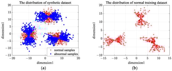
Figure 9.
The distribution of the second type of synthetic data and training samples. (a) The distribution of the second type of synthetic data; (b) the distribution of the training samples.

Figure 10.
The clustering result and classification boundary for the second type of synthetic dataset. (a) The initial clustering result; (b) the classification boundary.
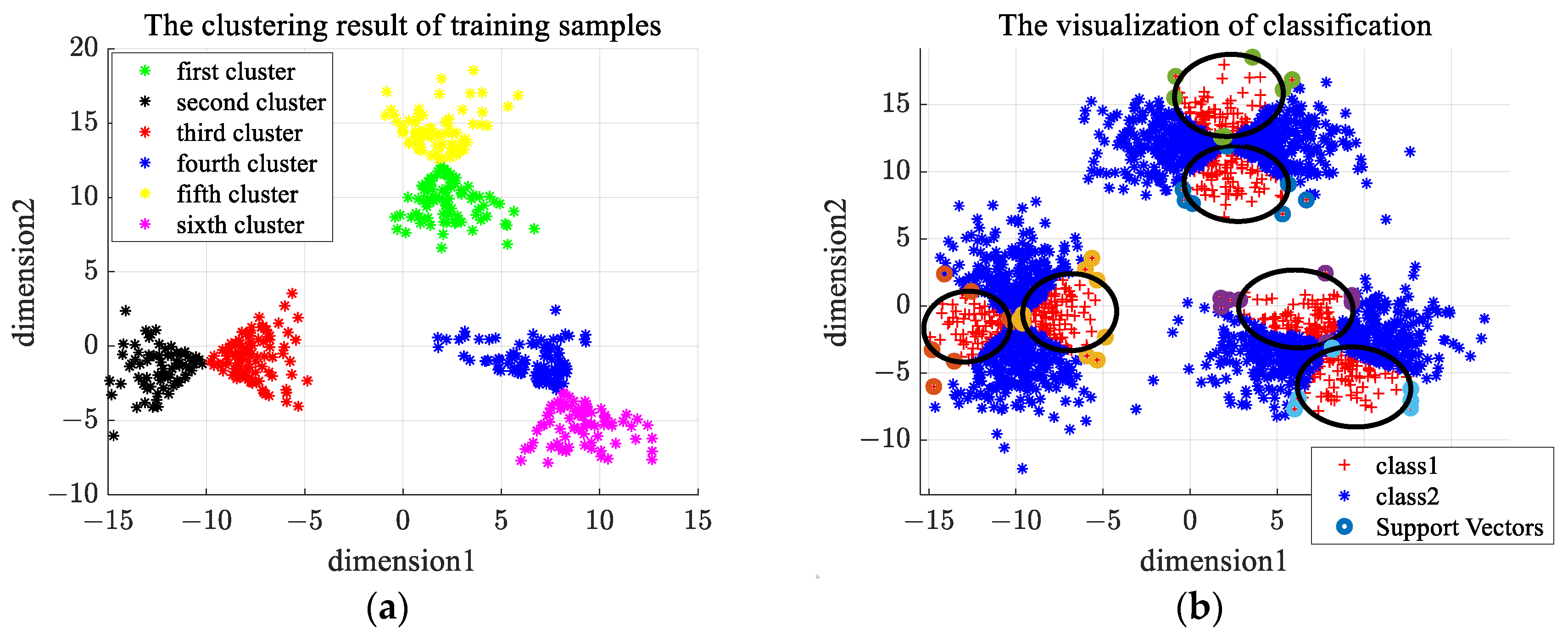
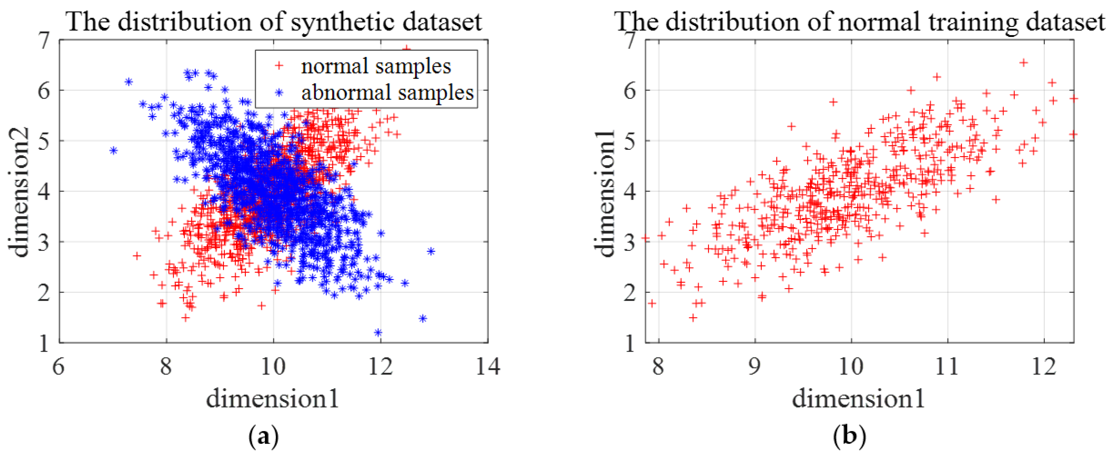
The distribution of the third type of synthetic data is shown in Figure 11a. We choose one class of samples as normal samples, and the distribution of training samples is shown in Figure 11b. The number of clusters in -means clustering is set as 2, and the rejection rate of training samples in OCSVM is set as 0.1. Figure 12a gives the clustering results of En-OCSVM, and the classification boundary of En-OCSVM is shown in Figure 12b. It can be seen from Figure 12a,b that the training samples were correctly clustered into two clusters. It can be seen from Figure 9 that although normal samples are classified correctly, abnormal samples in overlapping areas are misclassified.
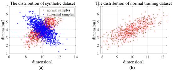
Figure 11.
The distribution of the third type of synthetic data and training samples. (a) The distribution of the third type of synthetic data; (b) the distribution of the training samples.
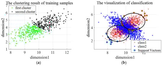
Figure 12.
The clustering result and classification boundary for the third type of synthetic dataset. (a) The initial clustering result; (b) the classification boundary.
Based on the Experimental results of these three synthetic datasets, we can conclude that if the distribution of normal and abnormal data in the feature space does not overlap, the proposed method can effectively distinguish the normal and abnormal data; on the contrary, the abnormal samples in the overlapping area will be misclassified.
4.3. Results on Benchmark Datasets
In this Section, we evaluate the performance of En-OCSVM on five benchmark datasets. Eight related methods are considered for comparison with the proposed method: Gaussian density estimation (Gauss) [16], PCA [21], -means clustering (k-means) [19], OCSVM with Gaussian kernel function (OCSVM) [23], Self-Organizing Map [35] (SOM), Auto-encoder (AE) neural network, one-class minimax probability machine [36] (MPM), and LOCSVM [24]. The values of the hyperparameter in -means clustering and the hyperparameter in the Gaussian kernel function are selected corresponding to the best performance for all methods via grid search. The range of values for the hyperparameter is [2, 5] with an interval of 1, and the range of values for the hyperparameter is [1, 10] with the interval of 0.1.
The performance of a one-class classifier (OCC) is evaluated with classification accuracy, i.e., the proportion between the number of samples that are correctly classified and the number of test samples. For clarity, we briefly denote to represent classification accuracy. In our experiments, the results are averaged over 10 random partitions of training and test datasets. The average values of are shown in Table 3 for all datasets. The average values of each method shown in Table 3 are averaged over its best results on each partition, which corresponds to the results with the optimal model parameters on each partition. The best overall performance for each criterion is shown in bold italics. We observe that the best performance in each column, i.e., for each criterion, is obtained by the proposed method.
Table 3.
Average classification accuracies (%) for three benchmark datasets over the 10 random partitions for the training and test sets.
To explain the importance of clustering further, the classification accuracies of En-OCSVM on five UCI datasets with different numbers of clusters are given in Figure 13a–e. We can see that the cluster number corresponding to the best results is greater than one on all datasets, which shows that it is meaningful to introduce -means clustering to OCSVM.
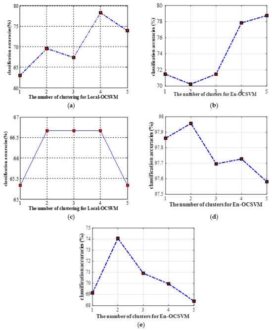
Figure 13.
The classification accuracies on different datasets with different numbers of clustering for En-OCSVM. (a) Glass dataset; (b) Parkinson dataset; (c) Splice dataset; (d) Pendigits dataset; (e) Waveform dataset.
4.4. Results on Sea Surface Datasets
In this section, we evaluate the performance of En-OCSVM on IPIX datasets. The comparison method and hyperparameter settings are the same as in Section 4.3. In the training step, 1000 clutter samples are randomly selected as a training set, and the remained clutter and target samples are used for testing. The performance of OCC is evaluated with three criteria: detection probability, false alarm, and classification accuracy. For clarity, we briefly denote , and to represent detection probability, false alarm, and classification accuracy respectively.
In our experiments, the results are averaged over 10 random partitions of training and test datasets. Table 4 and Table 5 are the detailed results of these two datasets. The best overall performance for each criterion is shown in bold italics. We observe that the best performance in each column, i.e., for each criterion, is obtained by the proposed method in most cases.
Table 4.
Average values (%) of three criteria for #54 data over the 10 random partitions for the training and test sets.
Table 5.
Average values (%) of three criteria for #311 data over the 10 random partitions for the training and test sets.
We can see from Table 4 and Table 5 that although the classification accuracies of all comparison methods are above 90%, our method obtains the highest results in detection probability and classification accuracy, while the false alarm is on an average level compared with other related methods, which demonstrates the effectiveness of En-OCSVM. Moreover, the results of the proposed method are better than OCSVM on all three criteria, which illustrates the importance of clustering.
To further demonstrate the reliability of the experimental results, the original features are reduced to 2 dimensions via PCA, and the 2D feature visualization results of reduced features for #54 and #311 data are shown in Figure 14a,b. We can see from Figure 14 that the distribution area of targets and clutter in the 2D feature plane is non-overlapping for #54 and #311 data. Therefore, the extracted features can effectively distinguish between targets and clutter, and the classification accuracy of each method is relatively high.
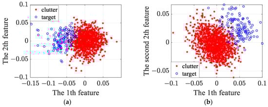
Figure 14.
The 2D visualization results of the reduced features for #54 and # 311 data. (a) #54 data; (b) #311 data.
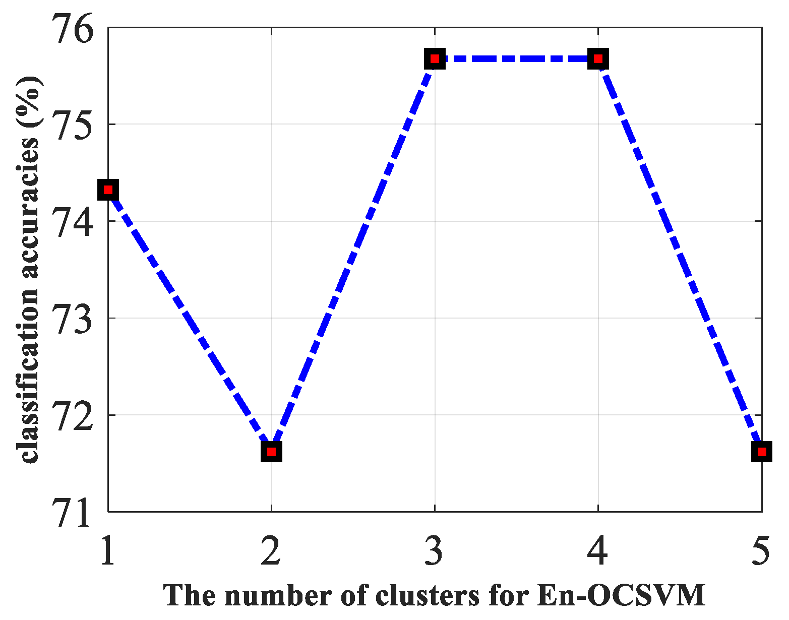
To explain the importance of clustering further, the classification accuracies of En-OCSVM on #54 data with different numbers of clusters are given in Figure 15. We can see that the clustering number corresponding to the best results is greater than one on this dataset, which shows that it is meaningful to introduce -means clustering to OCSVM.
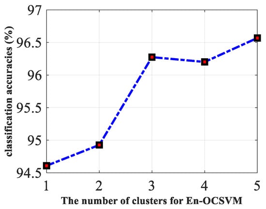
Figure 15.
The classification accuracies of En-OCSVM on #54 data with the different number of clusters.
4.5. Results on SAR Real Data
In Section 4.3 and Section 4.4, we present the performance of En-OCSVM on the benchmark dataset and sea surface datasets. Now, the performance of En-OCSVM on the SAR real data is shown in this Section. In our experiments, the number of training samples is 135, and the number of test samples is 74, including 45 target patches and 29 clutter patches. The model parameters’ settings are the same as those in the experiments on benchmark datasets. Similar to the experiments on the benchmark dataset, the results are averaged over 10 random partitions of training and test datasets. The performances, represented by the average values of the three criteria, are shown in Table 6. The best overall performance for each criterion is shown in bold italics. We can see from Table 6 that our method obtains the highest results and classification accuracy, and the detection probability of our method is suboptimal.
Table 6.
Average values (%) of three criteria for SAR real data over the 10 random partitions for the training and test sets.
To explain the importance of clustering further, the classification accuracies of En-OCSVM on SAR real data with different numbers of clusters are given in Figure 16. We can see that the cluster number corresponding to the best results is greater than one on this dataset, which shows that it is meaningful to introduce -means clustering to OCSVM.
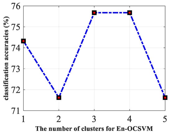
Figure 16.
The classification accuracies of En-OCSVM on SAR rea data with the different number of clusters.
5. Conclusions
In this paper, a novel one-class classification method, namely ensemble OCSVM (referred to as En-OCSVM), is proposed to enhance the performance of traditional one-class classifiers. En-OCSVM is a mixture model of -means clustering and OCSVM. In En-OCSVM, the training samples are clustered in the kernel space with -means clustering algorithm, while simultaneously a linear decision boundary is constructed in each cluster. The main contributions of this study are summarized below:
- Through the mixture of multiple linear decision boundaries, the complex nonlinear decision boundaries can be achieved in the kernel space, which can enhance the performance of OCSVM, especially when the distribution of data is complex.
- The joint optimization of -means clustering model and OCSVM model is realized based on support vectors (SVs) to guarantee the consistency of clustering and linear separability in each cluster.
The visualized experimental results on synthetic data explain the effectiveness and limitation of the proposed method, and the quantitatively experimental results on benchmark datasets, IPIX sea surface datasets and SAR real datasets demonstrate that our method outperforms traditional one-class classifiers. Like the other one-class classifiers, the proposed method can be used in fields such as anomaly detection, target detection, and target discrimination.
The shortcoming of En-OCSVM is that it is sensitive to model hyperparameters, such as the number of clustering and the Gaussian kernel parameter . Some reports in the literature [37,38,39] have studied how to adaptively select Gaussian kernel parameters in OCSVM, and some nonparametric Bayesian models (such Dirichlet process mixture model) can automatically determine the number of clusters when used for clustering. Therefore, we have the chance to solve the optimization problem of the value of and the Gaussian kernel parameter directly, and this will be studied in our future work. In addition, recently, Deep Neural Networks (DNNs) have achieved success in many applications since the ability of feature learning. Therefore, how to link DNNs with OCSVM could be a future research area.
Author Contributions
Conceptualization, S.C. and X.O.; methodology, S.C.; software, S.C.; validation, S.C., X.O., and F.L.; formal analysis, X.O.; investigation, X.O.; resources, F.L.; data curation, S.C.; writing—original draft preparation, S.C.; writing—review and editing, S.C.; visualization, S.C.; supervision, X.O.; project administration, F.L.; funding acquisition, F.L. All authors have read and agreed to the published version of the manuscript.
Funding
This work was supported by the National Natural Science Foundation of China (62201251), the Natural Science Foundation of the Jiangsu Higher Education Institutions of China (22KJB510024), and the Open Fund for the Hangzhou Institute of Technology Academician Workstation at Xidian University (XH-KY-202306-0291).
Data Availability Statement
The original contributions presented in the study are included in the article; further inquiries can be directed to the corresponding author.
Conflicts of Interest
The authors declare no conflicts of interest.
References
- Vapnik, V.N. An overview of statistical learning theory. IEEE Trans. Neural Netw. 1999, 10, 988–999. [Google Scholar] [CrossRef] [PubMed]
- Zhang, X.; Li, P.; Cai, C. Regional Urban Extent Extraction Using Multi-Sensor Data and One-Class Classification. Remote Sens. 2015, 7, 7671–7694. [Google Scholar] [CrossRef]
- Wan, B.; Guo, Q.; Fang, F.; Su, Y.; Wang, R. Mapping US Urban Extents from MODIS Data Using One-Class Classification Method. Remote Sens. 2015, 7, 10143–10163. [Google Scholar] [CrossRef]
- Fourie, C.; Schoepfer, E. Classifier Directed Data Hybridization for Geographic Sample Supervised Segment Generation. Remote Sens. 2014, 6, 11852–11882. [Google Scholar] [CrossRef]
- Liu, X.; Liu, H.; Gong, H.; Lin, Z.; Lv, S. Appling the One-Class Classification Method of Maxent to Detect an Invasive Plant Spartina alterniflora with Time-Series Analysis. Remote Sens. 2017, 9, 1120. [Google Scholar] [CrossRef]
- Zhang, J.; Li, P.; Wang, J. Urban Built-Up Area Extraction from Landsat TM/ETM+ Images Using Spectral Information and Multivariate Texture. Remote Sens. 2014, 6, 7339–7359. [Google Scholar] [CrossRef]
- Mack, B.; Waske, B. In-depth comparisons of MaxEnt, biased SVM and one-class SVM for one-class classification of remote sensing data. Remote Sens. Lett. 2017, 8, 290–299. [Google Scholar] [CrossRef]
- Ruff, L.; Vandermeulen, R.; Goernitz, N.; Deecke, L.; Siddiqui, S.A.; Binder, A.; Müller, E.; Kloft, M. Deep One-Class Classification. In Proceedings of the International Conference on Machine Learning, Stockholm, Sweden, 10–15 July 2018. [Google Scholar]
- Livi, L.; Sadeghian, A.; Pedrycz, W. Entropic One-Class Classifiers. IEEE Trans. Neural Netw. Learn. Syst. 2015, 26, 3187–3200. [Google Scholar] [CrossRef]
- Quinn, J.A.; Williams, C.K.I. Known unknowns: Novelty detection in condition monitoring. In Proceedings of the Iberian Conference on Pattern Recognition and Image Analysis, Girona, Spain, 6–8 June 2007; Springer: Berlin/Heidelberg, Germany, 2007; pp. 1–6. [Google Scholar]
- Tarassenko, L.; Clifton, D.A.; Bannister, P.R.; King, S.; King, D. Novelty Detection. In Encyclopedia of Structural Health Monitoring; John Wiley & Sons, Ltd.: Hoboken, NJ, USA, 2009. [Google Scholar]
- Surace, C.; Worden, K. Novelty detection in a changing environment: A negative selection approach. Mech. Syst. Signal Process. 2010, 24, 1114–1128. [Google Scholar] [CrossRef]
- Kemmler, M.; Rodner, E.; Rösch, P.; Popp, J.; Denzler, J. Automatic identification of novel bacteria using Raman spectroscopy and Gaussian processes. AnalyticaChimicaActa 2013, 794, 29–37. [Google Scholar] [CrossRef]
- Gambardella, A.; Giacinto, G.; Migliaccio, M.; Montali, A. One-class classification for oil spill detection. Pattern Anal. Appl. 2010, 13, 349–366. [Google Scholar] [CrossRef]
- Pimentel, M.A.F.; Clifton, D.A.; Clifton, L.; Tarassenko, L. A review of novelty detection. Signal Process. 2014, 99, 215–249. [Google Scholar] [CrossRef]
- Bishop, C. Pattern Recognition and Machine Learning (Information Science and Statistics), 1st ed.; Springer: New York, NY, USA, 2006; corr. 2nd printing edn. 2007. [Google Scholar]
- McLachlan, G.J.; Basford, K.E. Mixture models. Inference and applications to clustering. Stat. Textb. Monogr. N. Y. Dekker 1988, 1988, 1. [Google Scholar]
- Svensén, M.; Bishop, C.M. Robust Bayesian mixture modelling. Neurocomputing 2005, 64, 235–252. [Google Scholar] [CrossRef]
- Bishop, C.M. Neural Networks for Pattern Recognition; Oxford University Press: Oxford, UK, 1995. [Google Scholar]
- Hautamäki, V.; Kärkkäinen, I.; Fränti, P. Outlier detection using k-nearest neighbour graph. In Proceedings of the International Conference on Pattern Recognition, Cambridge, UK, 26 August 2004; IEEE: Piscataway, NJ, USA, 2004. [Google Scholar]
- Jolliffe, I. Principal Component Analysis; John Wiley & Sons, Ltd.: Hoboken, NJ, USA, 2002. [Google Scholar]
- Tax, D.; Duin, R. Support Vector Data Description. Mach. Learn. 2004, 54, 45–66. [Google Scholar] [CrossRef]
- Schölkopf, B.; Williamson, R.; Smola, A.; Shawe-TaylorÝ, J. SV estimation of a distribution’s support. Adv. Neural Inf. Process. Syst. 2000, 41, 582–588. [Google Scholar]
- Cyganek, B. One-Class Support Vector Ensembles for Image Segmentation and Classification. J. Math. Imaging Vis. 2012, 42, 103–117. [Google Scholar] [CrossRef]
- Platt, J. Sequential Minimal Optimization: A Fast Algorithm for Training Support Vector Machines. 1998. Available online: https://www.microsoft.com/en-us/research/publication/sequential-minimal-optimization-a-fast-algorithm-for-training-support-vector-machines/ (accessed on 21 May 2024).
- Shawe-Taylor, J.; Cristianini, N. Support Vector Machines and Other Kernel-Based Learning Methods; Cambridge University Press: Cambridge, UK, 2000. [Google Scholar]
- Manevitz, L.M.; Yousef, M. One-class svms for document classification. JMLR 2001, 2, 139–154. [Google Scholar]
- Unnthorsson, R.; Runarsson, T.P.; Jonsson, M.T. Model selection in one class nu-svms using rbf kernels. In Proceedings of the 16th Conference on Condition Monitoring and Diagnostic Engineering Management, Växjö, Sweden, 27–29 August 2003. [Google Scholar]
- Camci, F.; Chinnam, R.; Ellis, R. Robust kernel distance multivariate control chart using support vector principles. Int. J. Prod. Res. 2008, 46, 5075–5095. [Google Scholar] [CrossRef]
- Chen, Y.; Zhou, X.S.; Huang, T. One-class svm for learning in image retrieval. In Proceedings of the International Conference on Image Processing, Thessaloniki, Greece, 7–10 October 2001. [Google Scholar]
- Alashwal, H.; Deris, S.; Othman, R. One-class support vector machines for protein-protein interactions prediction. Int. J. Biomed. Sci. 2006, 1, 120–127. [Google Scholar]
- Li, D.-C. Feature-Based Detection Methods of Small Targets in Sea Clutter. Ph.D. Thesis, Xidian University, Xi’an, China, 2016. [Google Scholar]
- Shui, P.-L.; Li, D.-C.; Xu, S. Tri-Feature-Based Detection of Floating Small Targets in Sea Clutter. IEEE Trans. Aerosp. Electron. Syst. 2014, 50, 1416–1430. [Google Scholar] [CrossRef]
- Chang, C.-C.; Lin, C.-J. LIBSVM, a Library for Support Vector Machines. 2001. Available online: www.csie.ntu.edu.tw/~cjlin/libsvm (accessed on 1 December 2020).
- Kohonen, T.; Somervuo, P. Self-organizing maps of symbol strings. Neurocomputing 1998, 21, 19–30. [Google Scholar] [CrossRef]
- Ghaoui, L.E.; Jordan, M.I.; Lanckriet, G.R. Robust novelty detection with single-class MPM. In Proceedings of the Advances in Neural Information Processing Systems, Vancouver, BC, Canada, 9–14 December 2002; pp. 905–912. [Google Scholar]
- Liao, L.; Du, L.; Zhang, W.; Chen, J. Adaptive Max-Margin One-Class Classifier for SAR Target Discrimination in Complex Scenes. Remote. Sens. 2022, 14, 2078. [Google Scholar] [CrossRef]
- Wang, S.; Yu, J.; Lapira, E.; Lee, J. A modified support vector data description based novelty detection approach for machinery components. Appl. Soft Comput. 2013, 13, 1193–1205. [Google Scholar] [CrossRef]
- Xiao, Y.; Wang, H.; Xu, W. Parameter Selection of Gaussian Kernel for One-Class SVM. IEEE Trans. Cybern. 2015, 45, 927. [Google Scholar]


Disclaimer/Publisher’s Note: The statements, opinions and data contained in all publications are solely those of the individual author(s) and contributor(s) and not of MDPI and/or the editor(s). MDPI and/or the editor(s) disclaim responsibility for any injury to people or property resulting from any ideas, methods, instructions or products referred to in the content. |
© 2024 by the authors. Licensee MDPI, Basel, Switzerland. This article is an open access article distributed under the terms and conditions of the Creative Commons Attribution (CC BY) license (https://creativecommons.org/licenses/by/4.0/).