
Precise Orbit Determination for Maneuvering HY2D Using Onboard GNSS Data

Abstract
:1. Introduction
2. Quality Analysis of On-Board GNSS Observation Data
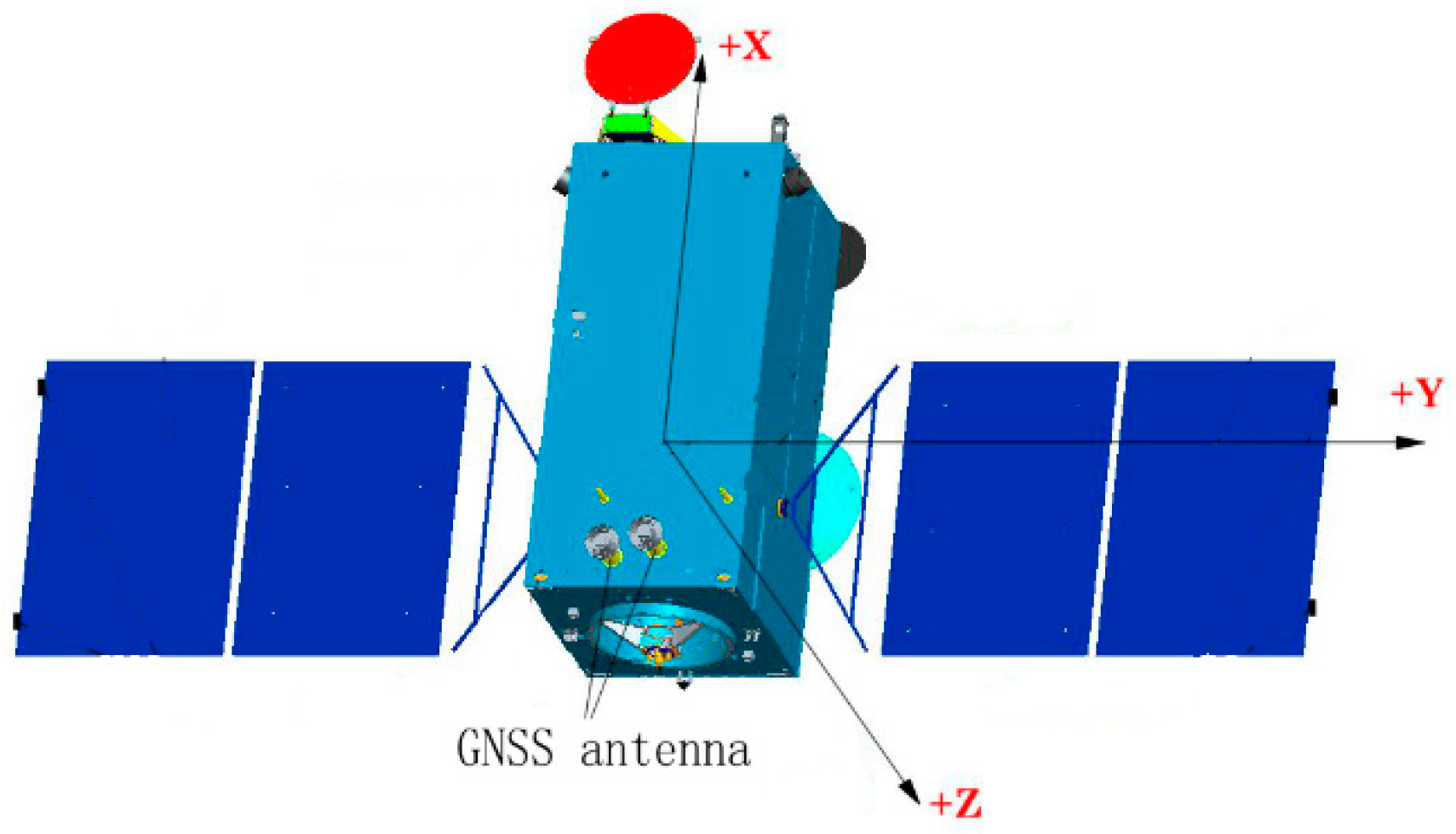
2.1. General Information about HY2D and Experimental Data
2.2. Analysis of Observation Data Quality
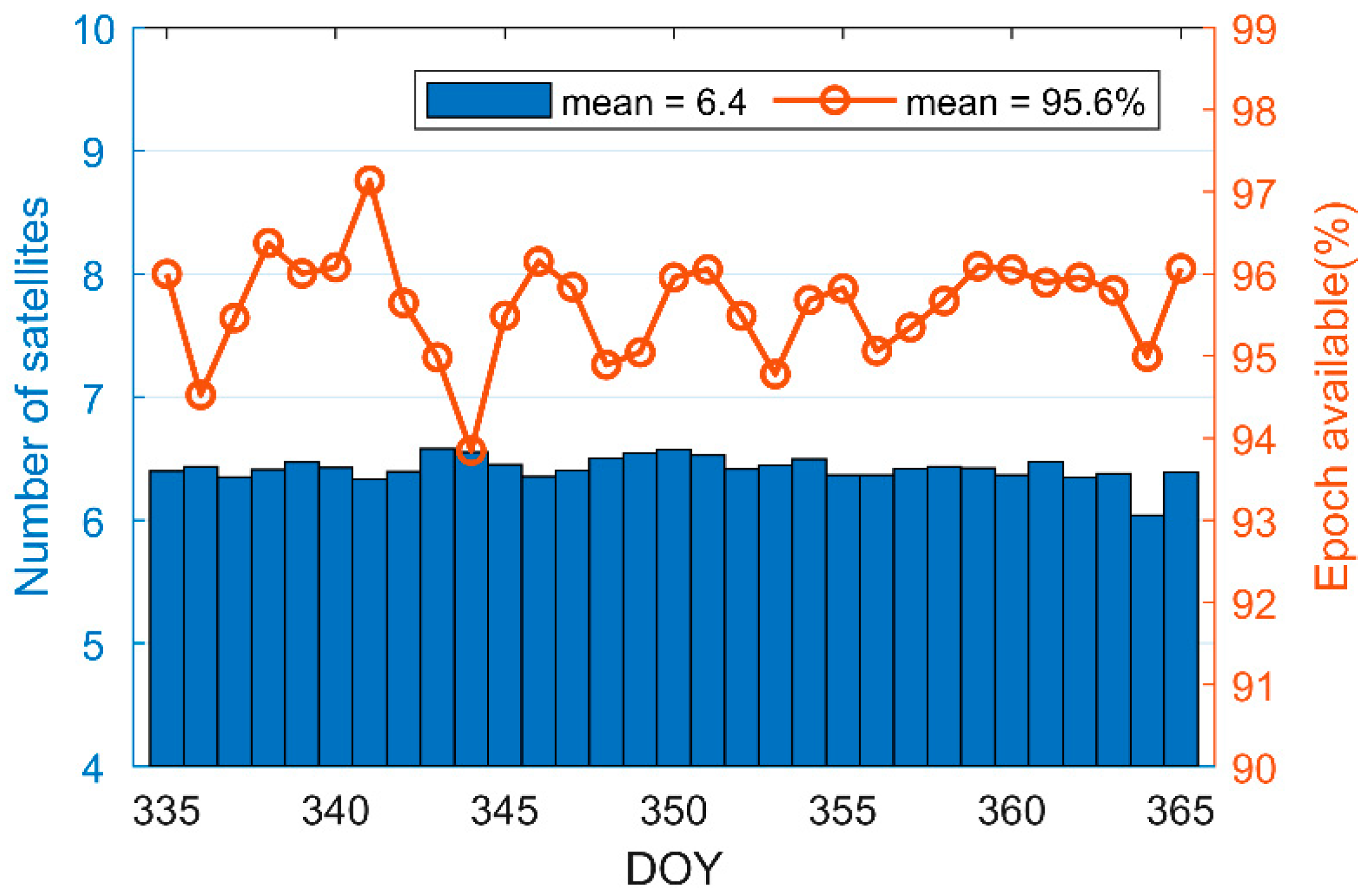
2.2.1. Effective Epoch
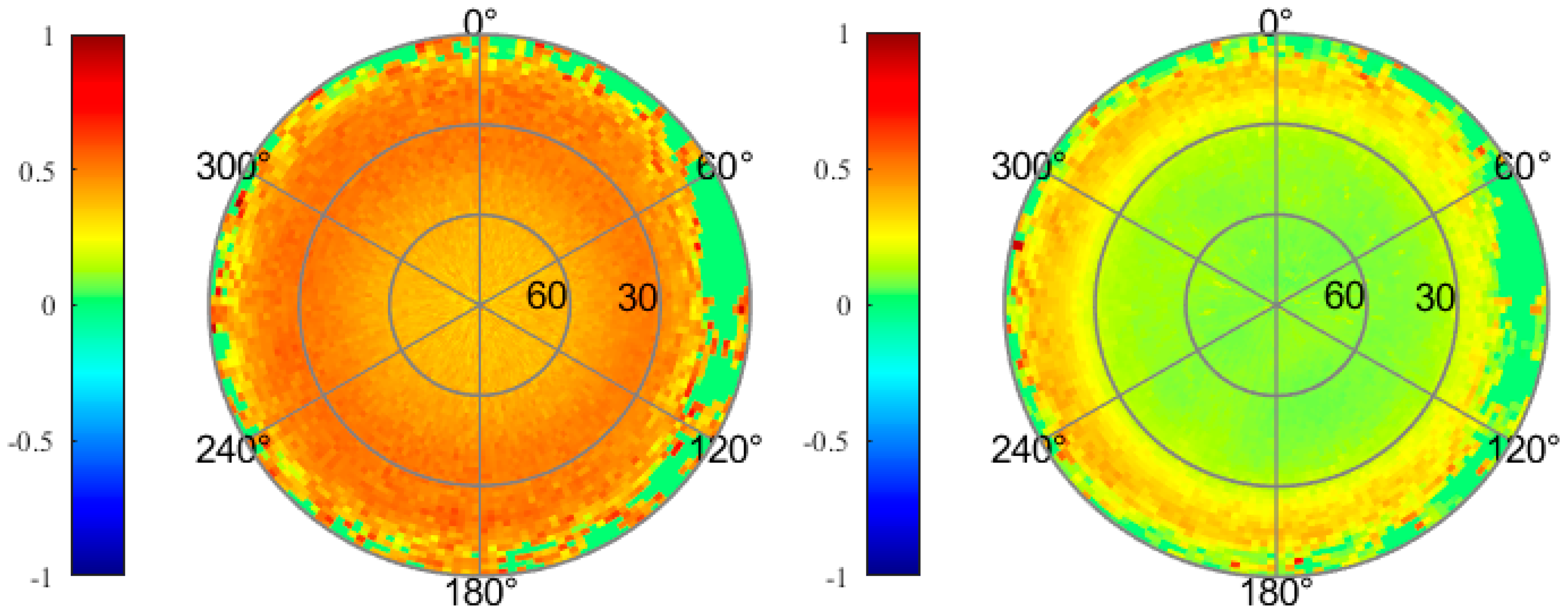
2.2.2. Multipath Effect
3. Precise Orbit Determination Strategies
3.1. Dynamic Model of POD
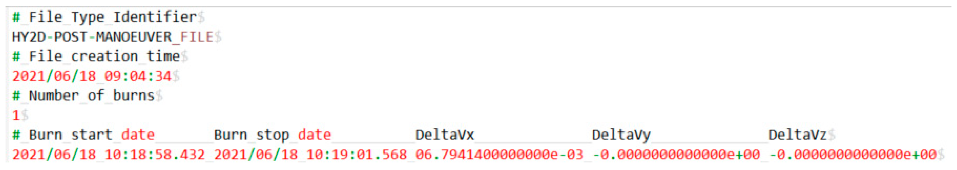
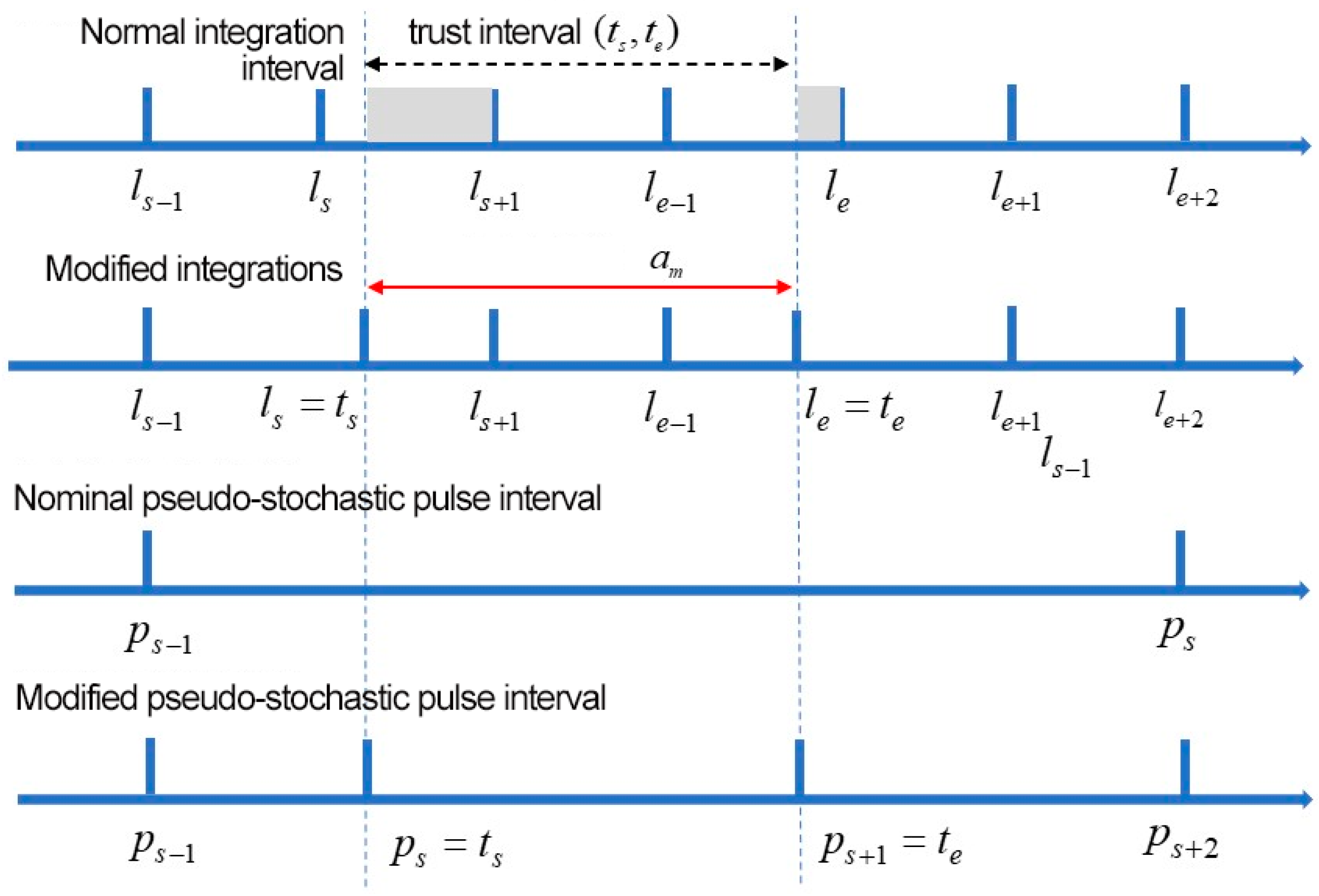
3.2. Maneuver Handling Strategy
4. Results and Discussion
4.1. Analysis of POD for Maneuvering HY2D
4.1.1. Carrier Phase Residuals Analysis for Maneuvering HY2D
4.1.2. Maneuver Assessment by POD
4.1.3. External Orbit Comparisons for Maneuvering HY2D
4.2. Orbit Validation and Analysis
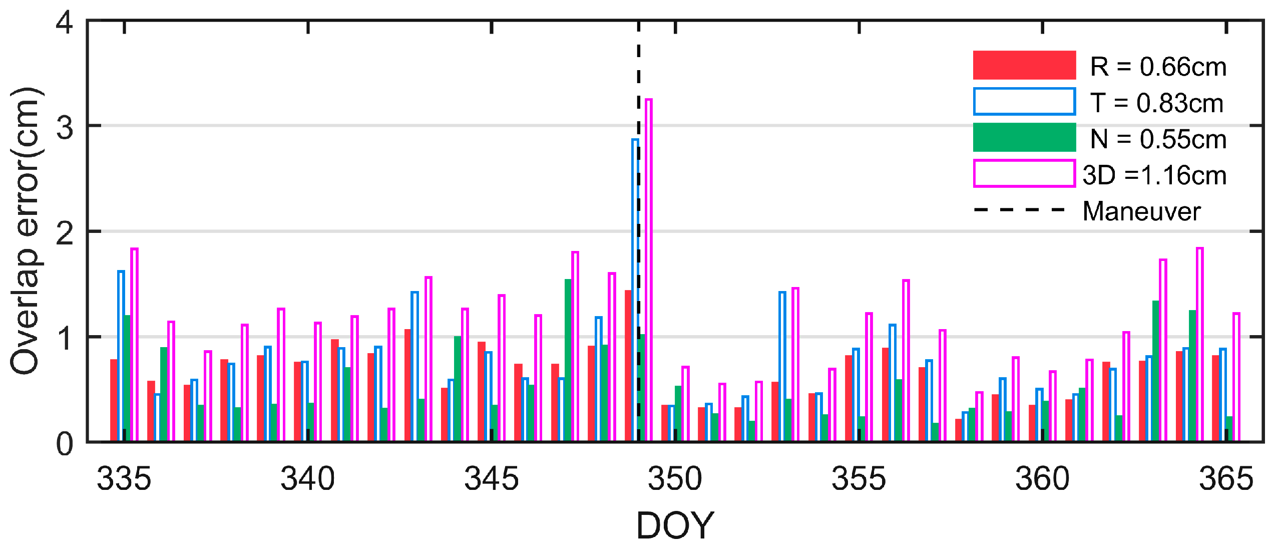
4.2.1. Overlap Comparison
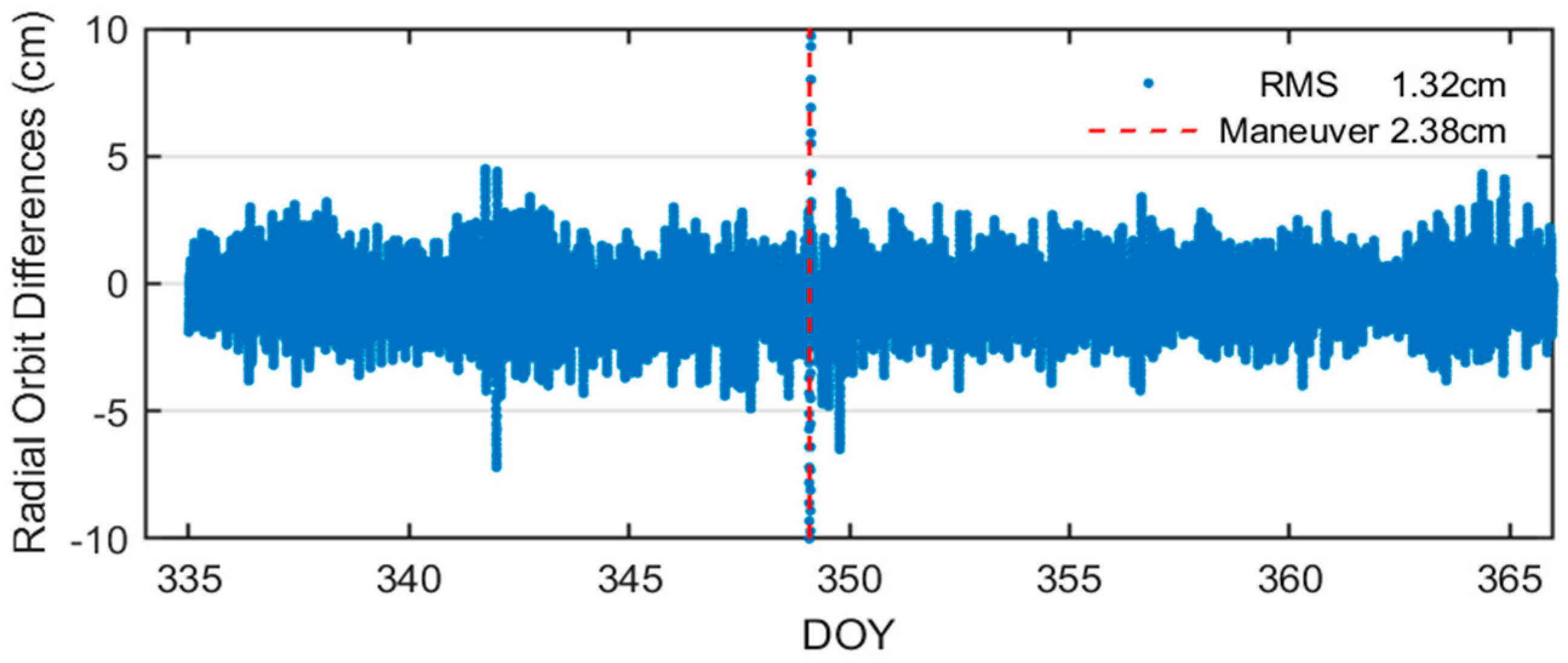
4.2.2. Comparison with Precision Science Orbits
4.2.3. SLR Range Validation
5. Conclusions
- (1)
- The on-board GNSS receiver demonstrates a strong tracking capability, with the number of satellites tracked per epoch ranging from 4 to 9, with an average of 6.4, and its code and phase observation data are of high quality.
- (2)
- In December 2023, during periods without satellite maneuvers, the average value of the RMS of the LC residuals is 0.7 cm; the average value of the RMS of the radial difference of the overlapping arc segments of the two adjacent days of 6 h is 0.66 cm; the difference of the 3D position is about 1.16 cm; the average RMS of the differences with the CNES standard orbital differences in the R, T, N, and 3D positions is 1.32 cm, 2.31 cm, 2.17 cm, and 3.53 cm, respectively.
- (3)
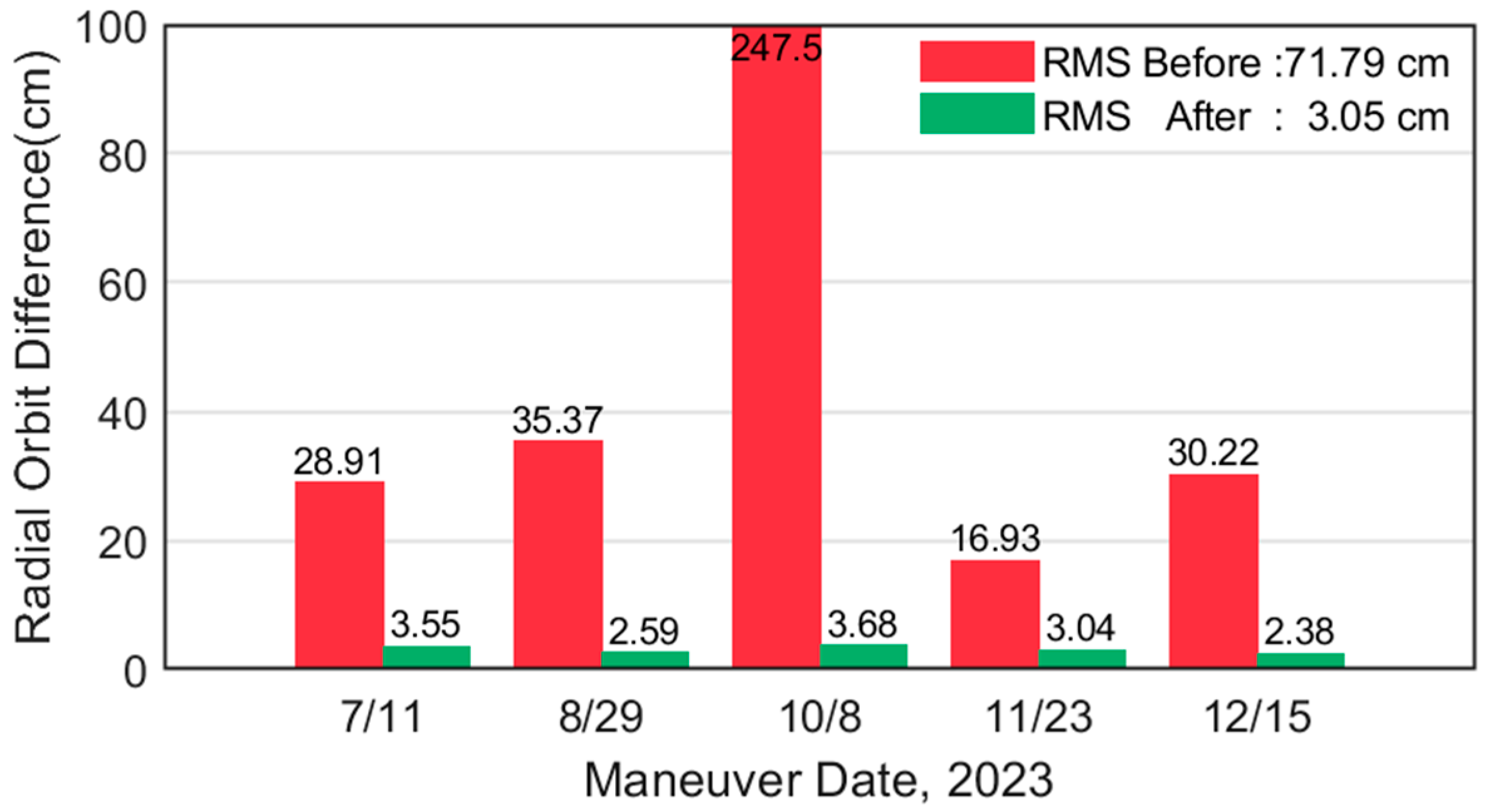
- The study selects five maneuver days in the second half of 2023 to validate the effect of the maneuver model strategy. The results show that maneuver handling can avoid precision degradation. For example, through the maneuvering treatment, the POD residuals are reduced from the original 1.93 cm to 0.79 cm, the orbit differences with PSO are reduced from the decimeter level or even the meter level to the centimeter level, and the average values of the R, T, and N differences of the orbit differences after maneuver handling are 3.04 cm, 8.78 cm, and 2.72 cm, respectively.
- (4)
- Using the global SLR core station data with an inter-station altitude angle greater than 20 degrees, the orbital accuracy in December 2023 (including the maneuver on December 15) is evaluated. The RMS of SLR residual differences in the ranging direction is 2.24 cm, indicating the effectiveness of the maneuver handling strategy and the significant improvement in orbit determination accuracy.
Author Contributions
Funding
Data Availability Statement
Acknowledgments
Conflicts of Interest
References
- Antony, J.W.; Gonzalez, J.H.; Schwerdt, M.; Bachmann, M.; Krieger, G.; Zink, M. Results of the TanDEM-X Baseline Calibration. IEEE J. Sel. Top. Appl. Earth Obs. Remote Sens. 2013, 6, 1495–1501. [Google Scholar] [CrossRef]
- Tapley, B.D. Gravity Model Determination from the GRACE Mission. J. Astronaut. Sci. 2008, 56, 273–285. [Google Scholar] [CrossRef]
- Jiang, K.; Li, M.; Zhao, Q.; Li, W.; Guo, X. BeiDou Geostationary Satellite Code Bias Modeling Using Fengyun-3C Onboard Measurements. Sensors 2017, 17, 2460. [Google Scholar] [CrossRef]
- Kang, Z.; Bettadpur, S.; Nagel, P.; Save, H.; Poole, S.; Pie, N. GRACE-FO Precise Orbit Determination and Gravity Recovery. J. Geod. 2020, 94, 85. [Google Scholar] [CrossRef]
- Fernández, M.; Aguilar, J.; Fernández, J. Sentinel-3 Properties for GPS POD, Copernicus Sentinel-1,-2 and-3 Precise Orbit Determination Service (SENTINELSPOD); GMV-GMESPOD-TN-0027, Version 1.7. 2019. Available online: https://sentinel.esa.int/documents/247904/322310/GMV-GMESPOD-TN-0027_v1.8_Sentinel-3+properties+for+GPS+POD.pdf/dda5b84b-6422-482b-a78c-a71e70679e9e (accessed on 29 June 2024).
- Jäggi, A.; Dahle, C.; Arnold, D.; Bock, H.; Meyer, U.; Beutler, G.; van Den Ijssel, J. Swarm Kinematic Orbits and Gravity Fields from 18 Months of GPS Data. Adv. Space Res. 2016, 57, 218–233. [Google Scholar] [CrossRef]
- Montenbruck, O.; Gill, E.; Lutze, F. Satellite Orbits: Models, Methods, and Applications. Appl. Mech. Rev. 2002, 55, B27–B28. [Google Scholar] [CrossRef]
- Peng, H.; Zhou, C.; Zhong, S.; Peng, B.; Zhou, X.; Yan, H.; Zhang, J.; Han, J.; Guo, F.; Chen, R. Analysis of Precise Orbit Determination for the HY2D Satellite Using Onboard GPS/BDS Observations. Remote Sens. 2022, 14, 1390. [Google Scholar] [CrossRef]
- Kecai, J.; Wenwen, L.; Min, L.; Jianghui, G.; Haixia, L.; Qile, Z.; Jingnan, L. Precise orbit determination of Haiyang-2D using onboard BDS-3 B1C/B2a observations with ambiguity resolution. Satell. Navig. 2023, 4, 28. [Google Scholar]
- Jäggi, A.; Montenbruck, O.; Moon, Y.; Wermuth, M.; König, R.; Michalak, G.; Bock, H.; Bodenmann, D. Inter-Agency Comparison of TanDEM-X Baseline Solutions. Adv. Space Res. 2012, 50, 260–271. [Google Scholar] [CrossRef]
- Zhang, H.; Gu, D.; Ju, B.; Shao, K.; Yi, B.; Duan, X.; Huang, Z. Precise Orbit Determination and Maneuver Assessment for TH-2 Satellites Using Spaceborne GPS and BDS2 Observations. Remote Sens. 2021, 13, 5002. [Google Scholar] [CrossRef]
- Allende-Alba, G.; Montenbruck, O.; Ardaens, J.-S.; Wermuth, M.; Hugentobler, U. Estimating Maneuvers for Precise Relative Orbit Determination Using GPS. Adv. Space Res. 2017, 59, 45–62. [Google Scholar] [CrossRef]
- Ju, B.; Gu, D.; Herring, T.A.; Allende-Alba, G.; Montenbruck, O.; Wang, Z. Precise Orbit and Baseline Determination for Maneuvering Low Earth Orbiters. GPS Solut. 2017, 21, 53–64. [Google Scholar] [CrossRef]
- Kai, S.; Houzhe, Z.; Xianping, Q.; Zhiyong, H.; Bin, Y.; Defeng, G. Precise Absolute and Relative Orbit Determination for Distributed InSAR Satellite System. Acta Geod. Cartogr. Sin. 2021, 50, 580. [Google Scholar]
- Mao, X.; Arnold, D.; Kalarus, M.; Padovan, S.; Jäggi, A. GNSS-Based Precise Orbit Determination for Maneuvering LEO Satellites. GPS Solut. 2023, 27, 147. [Google Scholar] [CrossRef]
- Beutler, G.; Jäggi, A.; Hugentobler, U.; Mervart, L. Efficient Satellite Orbit Modelling Using Pseudo-Stochastic Parameters. J. Geod. 2006, 80, 353–372. [Google Scholar] [CrossRef]
- Zhu, S.; Reigber, C.; König, R. Integrated Adjustment of CHAMP, GRACE, and GPS Data. J. Geod. 2004, 78, 103–108. [Google Scholar] [CrossRef]
- Dach, R.; Walser, P. Bernese GNSS Software Version 5.2; University of Bern: Bern, Switzerland, 2015. [Google Scholar]
- Pavlis, N.K.; Holmes, S.A.; Kenyon, S.C.; Factor, J.K. The Development and Evaluation of the Earth Gravitational Model 2008 (EGM2008). J. Geophys. Res. Solid Earth 2012, 117, B04406. [Google Scholar] [CrossRef]
- Lyard, F.H.; Allain, D.J.; Cancet, M.; Carrère, L.; Picot, N. FES2014 Global Ocean Tide Atlas: Design and Performance. Ocean Sci. 2021, 17, 615–649. [Google Scholar] [CrossRef]
- Petit, G.; Luzum, B. IERS Conventions. IERS Tech. Note 2010, 36, 2010. [Google Scholar]
- Folkner, W.M.; Williams, J.G.; Boggs, D.H. The Planetary and Lunar Ephemeris DE 421. IPN Prog. Rep. 2009, 42, 1. [Google Scholar]
- Bizouard, C.; Lambert, S.; Gattano, C.; Becker, O.; Richard, J.-Y. The IERS EOP 14C04 Solution for Earth Orientation Parameters Consistent with ITRF 2014. J. Geod. 2019, 93, 621–633. [Google Scholar] [CrossRef]
- Rodriguez-Solano, C.; Hugentobler, U.; Steigenberger, P. Adjustable box-wing model for solar radiation pressure impacting GPS satellites. Adv. Space Res. 2012, 49, 1113–1128. [Google Scholar] [CrossRef]
- Berger, C.; Biancale, R.; Barlier, F. Improvement of the empirical thermospheric model DTM: DTM94–a comparative review of various temporal variations and prospects in space geodesy applications. J. Geod. 1998, 72, 161–178. [Google Scholar] [CrossRef]
- Arnold, D.; Montenbruck, O.; Hackel, S.; Sośnica, K. Satellite Laser Ranging to Low Earth Orbiters: Orbit and Network Validation. J. Geod. 2019, 93, 2315–2334. [Google Scholar] [CrossRef]


| Item | X (mm) | Y (mm) | Z (mm) |
|---|---|---|---|
| COM location | 1319.4 | −4.7 | 5.7 |
| GPS phase center | 347.4 | −181.0 | −1396.1 |
| LRA spherical center | 311.7 | −215.5 | 1060.8 |
| Data | Organization | Related Addresses |
|---|---|---|
| On-board GPS observation data (1 s) | NSOAS | https://osdds.nsoas.org.cn (accessed on 29 June 2024) |
| On-board attitude angle data (1 s) | NSOAS | https://osdds.nsoas.org.cn (accessed on 29 June 2024) |
| GPS precise ephemeris (15 min) | CODE | http://ftp.aiub.unibe.ch/CODE (accessed on 29 June 2024) |
| GPS precise clock file (30 s) | CODE | http://ftp.aiub.unibe.ch/CODE (accessed on 29 June 2024) |
| Earth rotation parameters | CODE | http://ftp.aiub.unibe.ch/CODE (accessed on 29 June 2024) |
| HY2D precision orbit file (1 min) | CNES | https://ids-doris.org (accessed on 29 June 2024) |
| SLR observation data files | NASA | https://cddis.nasa.gov/archive/slr (accessed on 29 June 2024) |
| Serial Number | Date of Motorization | Day of the Year (DOY) | Start Time (UTC) | Duration (s) | Number of Thrusters |
|---|---|---|---|---|---|
| 1 | 11 July 2023 | 192 | 03:40:37.0 | 6.946 | 1 |
| 2 | 29 August 2023 | 241 | 03:00:37.0 | 5.778 | 1 |
| 3 | 8 October 2023 | 281 | 08:45:37.0 | 9.418 | 1 |
| 4 | 23 November 2023 | 327 | 01:40:37.0 | 5.688 | 1 |
| 5 | 15 December 2023 | 349 | 03:15:37.0 | 6.244 | 1 |
| Type | Model/Parameters | Description |
|---|---|---|
| Dynamic model | Gravity model | EGM2008 [19] |
| Ocean tide | FES2014 [20] | |
| Solid Earth tide | IERS 2010 Conventions [21] | |
| N-body perturbation | JPL DE421 [22] | |
| Earth orientation | IERS C04 [23] | |
| Relativity | IERS 2010 Conventions [21] | |
| Solar radiation | Box-Wing [24] | |
| Atmosphere drag | DTM94 [25] | |
| Empirical force | One-cycle-per-revolution acceleration (sine and cosine terms) in along-track and cross-track; | |
| Observation model | Observation | L1L2 |
| Arc length and interval | 30 h, 30 s | |
| Elevation cut-off angle (°) | 5° | |
| Precise ephemeris and clock | CODE precise final products | |
| GPS antenna PCO/PCV | IGS14.atx | |
| Estimated parameters | Initial state | Position and velocity at the initial epoch |
| Receiver clock offset | Epoch-wise clock offsets | |
| Phase ambiguities | Float | |
| Pseudo-stochastic pulses | One estimate every 15 min | |
| Maneuver accelerations | Estimated during the period of maneuver |
| Dates | DOY | Before Modeling (mm) | After Modeling (mm) | Improvement |
|---|---|---|---|---|
| 11 July 2023 | 192 | 16.6 | 7.2 | 56.63% |
| 29 August 2023 | 241 | 18.2 | 9.1 | 50.00% |
| 8 October 2023 | 281 | 28.8 | 7.8 | 72.92% |
| 23 November 2023 | 327 | 15.2 | 7.4 | 51.32% |
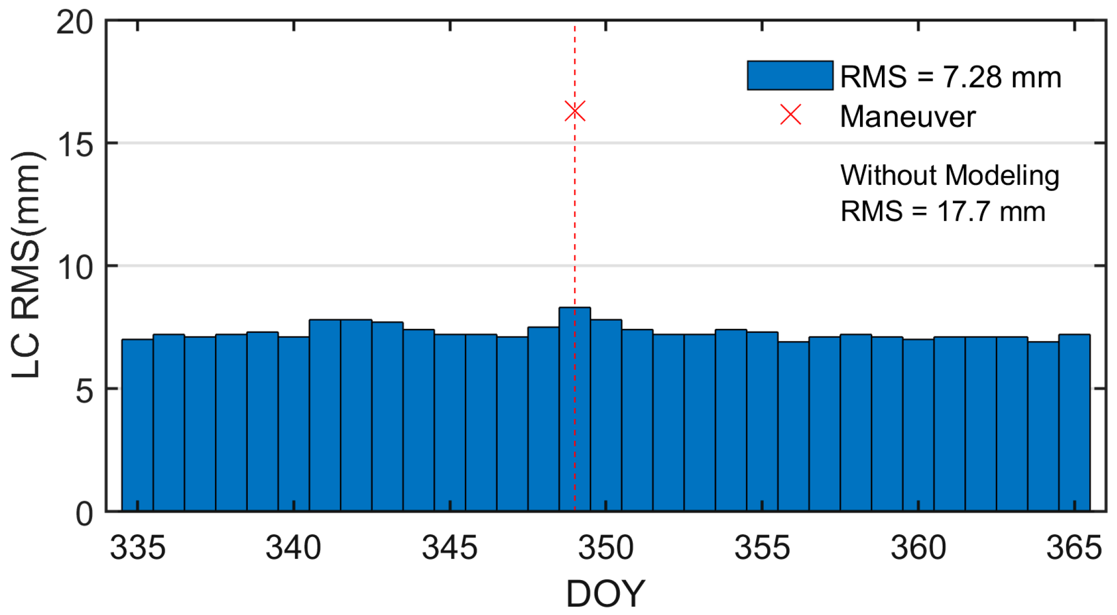
| 15 December 2023 | 349 | 17.7 | 7.9 | 55.37% |
| Date | Maneuver Information Delta v (m/s) | Solution Delta v (m/s) | Difference |
|---|---|---|---|
| 11 July 2023 | 1.25 × 10⁻² | 1.24 × 10⁻² | 0.80% |
| 29 August 2023 | 1.02 × 10⁻² | 0.94 × 10⁻² | 7.84% |
| 8 October 2023 | 1.68 × 10⁻² | 1.80 × 10⁻² | 7.14% |
| 23 November 2023 | 1.11 × 10⁻² | 0.90 × 10⁻² | 18.92% |
| 15 December 2023 | 1.11 × 10⁻² | 1.12 × 10⁻² | 0.90% |
| Periods | R (cm) | T (cm) | N (cm) |
|---|---|---|---|
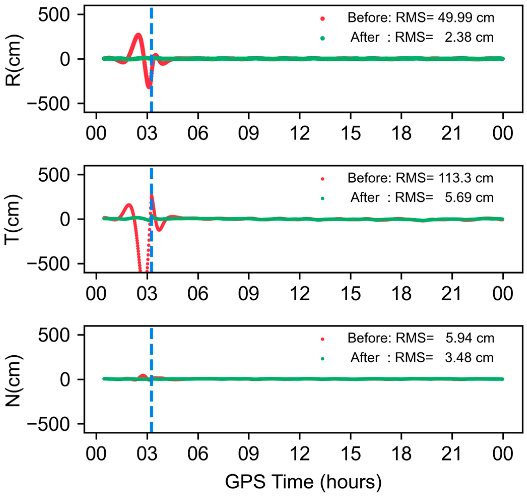
| maneuver | 2.38 | 5.89 | 3.48 |
| non-maneuver | 1.32 | 2.31 | 3.53 |
Disclaimer/Publisher’s Note: The statements, opinions and data contained in all publications are solely those of the individual author(s) and contributor(s) and not of MDPI and/or the editor(s). MDPI and/or the editor(s) disclaim responsibility for any injury to people or property resulting from any ideas, methods, instructions or products referred to in the content. |
© 2024 by the authors. Licensee MDPI, Basel, Switzerland. This article is an open access article distributed under the terms and conditions of the Creative Commons Attribution (CC BY) license (https://creativecommons.org/licenses/by/4.0/).
Share and Cite
Xu, K.; Zhou, X.; Li, K.; Wang, X.; Peng, H.; Gao, F. Precise Orbit Determination for Maneuvering HY2D Using Onboard GNSS Data. Remote Sens. 2024, 16, 2410. https://doi.org/10.3390/rs16132410
Xu K, Zhou X, Li K, Wang X, Peng H, Gao F. Precise Orbit Determination for Maneuvering HY2D Using Onboard GNSS Data. Remote Sensing. 2024; 16(13):2410. https://doi.org/10.3390/rs16132410
Chicago/Turabian StyleXu, Kexin, Xuhua Zhou, Kai Li, Xiaomei Wang, Hailong Peng, and Feng Gao. 2024. "Precise Orbit Determination for Maneuvering HY2D Using Onboard GNSS Data" Remote Sensing 16, no. 13: 2410. https://doi.org/10.3390/rs16132410