Interactions between MSTIDs and Ionospheric Irregularities in the Equatorial Region Observed on 13–14 May 2013

Abstract

We investigate the interactions between medium-scale traveling ionospheric disturbances (MSTIDs) and the equatorial ionization anomaly (EIA) as well as between MSTIDs and equatorial plasma bubbles (EPBs) on the night of 13–14 May 2013, based on observations from multiple instruments (an all-sky imager, digisonde, and global positioning system (GPS)). Two dark bands (the low plasma density region) for the MSTIDs were observed moving toward each other, encountering and interacting with the EIA, and subsequently interacting again with the EIA before eventually dissipating. Then, a new dark band of MSTIDs moved in the southwest direction, drifted into the all-sky imager’s field of view (FOV), and interacted with the EIA. Following this interaction, a new dark band split off from the original dark band, slowly moved in the northeast direction, and eventually faded away in a short time. Subsequently, the original southwestward-propagating dark band of the MSTIDs encountered eastward-moving EPBs, leading to an interaction between the MSTIDs and the EPBs. Then, the dark band of the MSTIDs faded away, while the EPBs grew larger with a pronounced westward tilt. The results from various observational instruments indicate the pivotal role played by the high-density region of the EIA in the occurrence of various interaction processes. In addition, this study also revealed that MSTIDs propagating into the equatorial region can significantly impact the morphology and evolution characteristics of EPBs.

1. Introduction

There are mainly three types of ionospheric phenomena after sunset in low-latitude ionospheric F regions: medium-scale traveling ionospheric disturbances (MSTIDs), the equatorial ionization anomaly (EIA), and equatorial plasma bubbles (EPBs). MSTIDs typically occur in mid-latitude regions, and Perkins instability and gravity waves are considered to be the primary mechanisms for their generation [1,2,3]. In the Northern (Southern) Hemisphere, their phase fronts usually align from the northwest (northeast) to the southeast (southwest) direction and propagate southwest (northwest) [4,5,6,7,8,9]. Most of the MSTIDs observed in low-latitude regions are believed to be primarily propagations of mid-latitude-originating MSTIDs [10,11,12]. The EIA is a large structure in the F region of the ionosphere near the magnetic equator which typically consists of two ionospheric ionization crests near ±15° magnetic latitudes and an ionization trough near the magnetic equator [13,14,15]. Its formation is usually explained by the ‘fountain effect’ resulting from vertical plasma drifts and diffusion [13,16]. The EPBs primarily occur in the low-latitude F region after sunset, with their main generation mechanism being attributed to the equatorial region’s Rayleigh–Taylor instability (RTI) [17,18]. They typically move from west to east [19,20,21,22]. The formation mechanism and evolutionary characteristics of these ionospheric structures have been extensively studied [7,8,9,15,23,24,25,26,27,28,29,30,31,32,33,34,35,36,37,38,39].

In recent years, the interaction of these ionospheric structures has become a topic of research interest. Interaction between MSTIDs and EPBs is one of the most extensively studied aspects. Many studies have found that MSTIDs propagating toward the equatorial region can induce disturbances at the bottom of the ionospheric F region, thereby contributing to the generation of EPBs [40,41]. There have also been a few studies reporting interactions between MSTIDs and eastward-moving EPBs, with subsequent gradual dissipation of EPBs being attributed to the polarization electric field induced by MSTIDs, causing the surrounding plasma to fill the interior of the EPBs [38,42]. In addition, the EIA structure is considered to be a source hindering the propagation of MSTIDs [12,43]. Previous studies found that EIA crests often impede the propagation of MSTIDs. This is believed to be a major reason why most mid-latitude MSTIDs cannot propagate to lower latitudes [12,44]. However, rather few studies have reported interactions between MSTIDs. It was found that MSTID structures often change their morphologies and propagation directions after such interactions. These changes have been attributed to polarization electric field effects within the internal structures of MSTIDs [38,45]. With the increase in studies related to MSTIDs, some abnormal MSTIDs are gradually being reported. For example, some studies have found Northern Hemisphere MSTIDs that did not propagate southwestward [12,38,46]. The mechanisms behind the occurrence of MSTIDs in low-latitude and equatorial regions are currently not clear. The interactions between low-latitude MSTIDs and ionospheric irregularities remain a quite interesting research topic due to the complexity of these interactions. The complex interaction processes and physical mechanisms require further investigation. On 13–14 May 2013, an all-sky imager observed complex interactions of MSTIDs with MSTIDs, MSTIDs with the EIA, and MSTIDs with EPBs, providing favorable conditions to study the mechanisms, evolution, and interactions of MSTIDs, the EIA, and EPBs.

In this study, we present the interactions between MSTIDs and various ionospheric structures in the equatorial region on the night of 13–14 May 2013 by using the all-sky imager data as well as concurrent digisonde data and global positioning system (GPS) data. Each interaction process is analyzed in detail.

2. Materials and Methods

The observational data used in the study were obtained from four instruments: an all-sky imager, a digisonde, and two GPS receivers. The all-sky imager and digisonde were located at the Fuke station (geographic coordinates: 19.5°N, 109.1°E; geomagnetic latitude: 9.5°N) in China. The all-sky imager mainly consists of a 180° FOV fisheye lens, a 630 nm filter, and a charge-coupled device detector of 1024 × 1024 pixels. Relevant data from this all-sky imager have been utilized in many studies on ionospheric irregularities, and detailed information has been described in previous studies [32,47,48,49]. The vertical total electron content (VTEC) data were obtained from the GPS receivers at the Sanya (geographic coordinates: 18.3°N, 109.6°E; geomagnetic latitude: 8.8°N) and Wuhan (geographic coordinates: 30.5°N, 114.3°E; geomagnetic latitude: 20.6°N) stations.

3. Results

Figure 1 shows a series of airglow observation images obtained from the Fuke station on the night of 13–14 May 2013 between 10:14 p.m. and 3:00 a.m. local time (LT). It was a quiet day (maximum|Dst| < 20). Based on the unwarping process of Garcia et al. [50], the effects of compression and curving of the all-sky lens were removed, and we mapped each image into a uniform geographic coordinate system (from 101° to 117°E longitude and from 11.5° to 27.5°N latitude) under the assumption that the height of the airglow emission layer was 250 km. The right of each image was to the east, and the top was to the north. The red circle in each image represents the FOV of the digisonde at an altitude of 250 km.

The observation results in Figure 1 show the interaction processes of various ionospheric irregularities on the night of 13–14 May 2013. In low-latitude regions, the all-sky imager (630 nm filter) typically observes two types of ionospheric irregularities: MSTIDs and EPBs. We usually distinguish them based on their morphologies and propagation characteristics. In the Northern Hemisphere, MSTIDs typically align from northwest to southeast and propagate southwestward or northeastward [4,5,6,7,8,9]. The structures marked by the yellow dashed lines in Figure 1 exhibited such characteristics, indicating that these structures were MSTIDs. On the other hand, EPBs generally align from north to south and move from west to east [19,20,21,22]. The structures marked by the red dashed lines in Figure 1 exhibited the same characteristics, indicating that these structures were EPBs. After approximately 10:23 p.m. LT, a series of MSTIDs appeared in the FOV of the all-sky imager. We used T0, T1, and T2 to mark the dark bands within the MSTIDs. The dark band T0 propagated toward the northeast, while the dark band T1 propagated toward the southwest. (It was not easy to determine T0, T1, and their propagations in Figure 1 alone, but they can be clearly distinguished in Supplementary Material Movie S1.) At approximately 11:00 p.m. LT, T1 encountered T0, marking the first interaction in this event (the detailed interaction process can be viewed in Supplementary Material Movie S1). The interaction of the two dark bands (T0 and T1) resulted in the formation of a new dark band, T0-1, which continued to move southwestward. Subsequently, a new dark band, T2, drifted into the FOV and followed T0-1 as it moved southwest. At approximately 12:00 a.m. LT, these two dark bands entered a region with an extremely high plasma density (likely the EIA crest, as the TEC value was ~53 TECU; see the TEC observations later), and they started to interact with the high-density plasma. After this interaction process, T0-1 gradually faded away after 12:31 a.m. LT. However, an interesting phenomenon occurred with T2 after the interaction. After ~1:32 a.m. LT, a new dark band, T2a, split off from the eastern side of T2. T2 continued to propagate southwestward, while T2a moved northeast and rapidly dissipated within 30 min. More interestingly, after ~1:53 a.m. LT, T2 encountered two eastward-moving EPBs (b1 and b2). After interacting with the EPBs, T2 gradually faded away after ~2:11 a.m. LT. Conversely, the EPBs exhibited faster growth (poleward extension) after the interaction (after ~2:11 a.m. LT), extending more rapidly to the north while also showing a pronounced westward tilt. For better understanding of the airglow observation results described above, we show a schematic diagram of several main interactions in Figure 2. In Figure 2, the black regions represent MSTID structures corresponding to Figure 1, the red regions represent EPB structures, and the yellow regions represent the main EIA crest regions. (Subsequent TEC observations suggest that the main EIA crest in this region was mainly located near 20°N).

Figure 3 shows the ionograms during the night of 13–14 May 2013. The ionograms are from the digisonde located at the Fuke station between 10:00 p.m. and 2:45 a.m. LT. The time interval between each image was 15 min. In Figure 3, spread F began to appear after ~10:45 P.M. LT, although it was relatively weak. It continued to exist until 2:45 A.M. LT, and its presence aligned closely with the time when ionospheric irregularities were observed through airglow observations. The lack of an obvious spread F before 10:45 p.m. LT was due to the narrow observation FOV of the digisonde (the red circles in Figure 1 represent the FOV of the digisonde at an altitude of 250 km), and thus the MSTIDs might not have drifted into its FOV yet. Figure 1 also shows that before ~10:45 p.m. LT, no irregularities drifted into the FOV of the digisonde. After ~10:45 p.m. LT, T0 gradually drifted into the FOV of the digisonde. Furthermore, irregularities continuously appeared within the FOV of the digisonde. This corresponds with the observational results shown in Figure 3. It is worth noting that at ~1:30 a.m. LT, there were clear observations of strong sporadic E (Es) activity, which continued until ~2:30 a.m. LT. After that, the strong Es activity gradually dissipated.

Figure 4 shows simultaneous GPS-TEC observations during the night of 13–14 May 2013. The pseudorandom numbers (PRNs) 2, 3, 10, 17, and 28 from the Sanya station and PRNs 4 and 10 from the Wuhan station were used to track these ionospheric phenomena in the event. In each image of Figure 4, the trajectories of the ionospheric pierce points (IPPs) of the GPS signals were mapped onto the airglow images. The IPP trajectories of PRNs 2, 3, 10, 17, and 28 from the Sanya station and the IPP trajectories of PRNs 4 and 10 from the Wuhan station are marked with blue and black lines, respectively, with red dots indicating the positions of the IPPs corresponding to the times of the airglow images. Figure 5 shows the vertical TEC (VTEC) variations for each PRN corresponding to the IPP trajectories in Figure 4 from 10:00 p.m. to 3:00 a.m. LT on 13–14 May 2013. In Figure 4 and Figure 5, these IPP trajectories for the PRNs from the Sanya station passed through the airglow FOV during that time period, while those from the Wuhan station mainly passed through the northeastern region outside of the airglow FOV. For the PRNs from Sanya, PRNs two and three primarily detected T0-1 and T2. Near 12:00 a.m. LT, the IPP trajectories of PRNs two and three entered the T0-1 plasma depletion region, corresponding to the first trough in VTEC in Figure 5. Then, the IPP trajectories of PRNs two and three detected a significant increase in VTEC near ~1:00 a.m. LT, corresponding to a high-density region on the east side of T0-1. Following that, the IPP trajectories of PRNs two and three entered the T2 plasma low-density region, and a second noticeable trough in VTEC appeared. When compared with PRN three, PRN two exhibited a third prominent VTEC trough. This is because after ~1:30 a.m. LT, the IPP trajectories of PRN two entered the T2a region, detecting the split MSTID dark band. For PRN 10, it detected T0-1 at ~12:30 a.m. LT and subsequently entered a high-density region on the east side of T0-1, resulting in a significant increase in VTEC. Finally, it entered the T2 region, where the VTEC gradually decreased. Similarly, PRN 17 first detected T0-1, followed by detecting a high-density region to the east, and then it entered the T2 low-density region, leading to a gradual decrease in VTEC. Although PRN 28 did not pass through any MSTID or EPB regions, its IPP trajectories moved from near 20°N toward the magnetic equator. The VTEC variation showed a noticeable decrease over time, which indicates that the region near 20°N is a high-density plasma region: the EIA crest. Although the PRNs from Wuhan did not pass through the airglow FOV, they provided important information for understanding the origins of the MSTIDs. For the PRNs 4 and 10 from Wuhan, a significantly high VTEC structure was observed around 11:00 p.m. LT. This corresponds to the high-density region of the MSTIDs following T0-1, which later entered the airglow FOV. It also enhanced the VTEC region detected to the east of T0-1 through the PRNs from the Sanya station. In the VTEC results of Wuhan’s PRN four, other distinct VTEC peaks and troughs were detected after the high-density region at 11:00 p.m. LT, demonstrating the presence of MSTIDs in that region. This indicates that the southwest-propagating MSTIDs observed in the airglow FOV were propagated from the northeastern region outside of the airglow FOV. For the VTEC results for Wuhan’s PRN 10, almost no distinct MSTID structures were presented after 12:00 a.m. LT. This was due to the fact that, at this later time, the IPP trajectories of PRN 10 were almost parallel to the phase of the MSTIDs.

4. Discussion

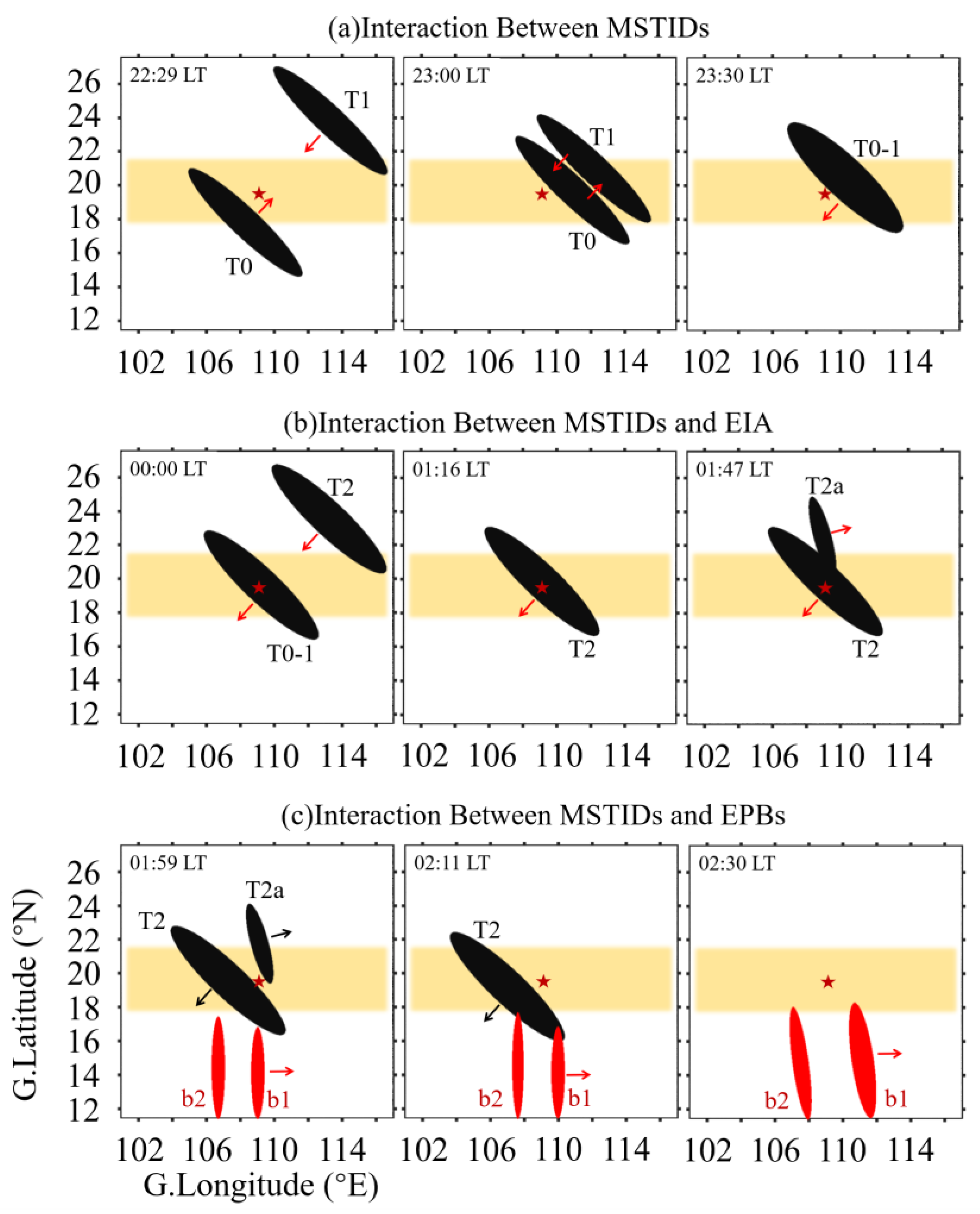
4.1. The Interaction between MSTIDs and the EIA

The interaction between MSTIDs in this event was similar to that in a previous study by Wu et al. [38], and thus it will not be discussed further here. In this study, we mainly focused on the interactions between MSTIDs and the EIA as well as EPBs. The interaction between MSTIDs and the EIA is an important research topic. Some studies have already found that most mid-latitude MSTIDs propagating toward the equator cannot cross the EIA region [12,44,51]. In this study, T0 and T1 were hindered over the station by the northern EIA crest. Other studies found that some MSTIDs can propagate into regions quite close to the magnetic equator [10,12,18,51,52]. Thus, the interaction between MSTIDs and the EIA typically results in two outcomes; one is that MSTIDs continue to propagate toward the equatorial region after crossing the EIA crest, and the other is that they are hindered by the EIA crest and eventually dissipate near the EIA crest. In our study, the interactions between T0, T1, T0-1, and the EIA all fell into the second category. As described in previous studies, the high-density region of the EIA can increase ion drag while suppressing polarization electric fields, thereby restricting the propagation of MSTIDs [43,44,53,54]. Since both T0 and T1 propagated to the high-density region of the EIA, and the high-density region of the EIA hindered their further propagation forward, and this resulted in T0 and T1 being unable to cross the EIA region. After being hindered by the EIA, an interaction between T0 and T1 occurred, forming T0-1. Subsequently, T0-1 gradually dissipated after midnight.

What is even more interesting is that after the disappearance of T0-1, the subsequent MSTID dark band, T2, interacted once again with the EIA. However, T2 did not immediately dissipate. Instead, during its interaction with the EIA, a branch, T2a, emerged to the northeast of T2. This branch gradually separated from T2 and moved in a reverse direction to the northeast for some time before eventually fading away. There have been few studies that reported the occurrence of branched structures in MSTIDs [55,56]. However, to the best of our knowledge, no one has reported the splitting off of a branched structure from an MSTID structure. In previous research, the mechanism for the branching of an MSTID dark band was usually attributed to secondary gradient drift instabilities during the interaction process. The airglow images represent a crude map of the integrated Pedersen conductivity (${\sum }_p$) [57]. The depletion region represents low${\sum }_p$, while enhancement represents high${\sum }_p$. In order to keep J (∇ • J = 0), low${\sum }_p$ must have a larger electric field than the adjacent high${\sum }_p$ [6]. Thus, when the low plasma density of MSTIDs encounters the EIA, low plasma density (low${\sum }_p$) will develop large eastward polarization fields, which cause more rapid upward or poleward flows than in the background plasma [6,53]. Then, when the eastward polarization electric field acts on the northward plasma gradient region of the MSTID in the low-density region of the EIA, secondary gradient drift instabilities can trigger new branching [53,55]. In our study, the emergence process and location of the T2a branch were similar to the previous results. Thus, we can believe that its generation mechanism should mainly originate from the secondary gradient drift instabilities described in those previous studies. However, what differs from the previous studies is that the branching later split off. One possible reason for this is that to the southwest of T2, the high-density region (the high-density region in front of T2 in Figure 1) of the MSTIDs was blocked by the EIA and enhanced the EIA, strengthening the secondary gradient drift instabilities in that region, which ultimately caused T2a to split off to the northeast. Then, T2a interacted again with the EIA, and it was swiftly smoothed out by the high-density EIA region.

4.2. The Interaction between MSTIDs and EPBs

Many studies have found that MSTIDs can seed or influence RTI development, thereby affecting the occurrence or evolution of EPBs [40,41]. A study by Miller et al. [40] based on airglow and VHF radar observations showed that polarization electric fields associated with MSTIDs can seed the development of EPBs when entering low-latitude regions. Krall et al. [41] used SAMI3/ESF model simulations and found that coupling between an MSTID at low-to-middle latitudes and the equatorial F layer led to growth in EPBs. In addition to their ability to trigger EPBs, some studies also reported MSTIDs interacting with EPBs encountered during MSTID propagation. Otsuka et al. [42] and Wu et al. [38], based on airglow observations, reported the gradual decay of EPBs following encounters with MSTIDs. They attributed this interaction to the polarization electric field within MSTID structures, which resulted in the surrounding plasma filling the EPB structures. On the other hand, a limited number of studies have also found that when MSTIDs encountered EPBs, the polarization electric field within the MSTID structure could reactivate fossil EPBs [49,58]. However, in our study, the interaction between MSTIDs and EPBs was more complex and differed from previous studies. The EPBs did not fossilize before encountering MSTIDs, and after the interaction, they did not disappear; instead, they grew faster toward higher latitudes, accompanied by more pronounced depletion, and they exhibited distinct distortion at higher latitudes. In contrast, the MSTID dark band rapidly dissipated after interacting with the EPBs. The physical mechanisms of this interaction process warrant further investigation.

For the MSTIDs, they were located in the EIA crest region when they encountered EPBs. For growing EPBs, there are polarization electric fields within them [59,60]. The zonal component of the electric fields causes plasma to drift upward, while the vertical component of the electric fields causes plasma to drift along the zonal direction [61]. During the interaction, it is possible that due to the growth and drift EPBs, these electric fields push surrounding plasma into the low-density regions of the MSTIDs, ultimately resulting in the gradual disappearance of T2 of the MSTIDs and an increase in plasma dissipation within the EPBs. As for the sudden increase in the growth rate of EPBs, this is attributable to the emergence of an enhanced eastward electric field in the region following the interaction. Studies from Carrasco et al. [61] and Otsuka et al. [42] indicated that during the interaction of EPBs, associated changes in the electric field could cause abrupt growth of EPBs. Wrasse et al. [58] also showed that during the interaction between MSTIDs and EPBs, the enhancement of the eastward electric field plays an important role in the growth of EPBs. This eastward electric field, through E×B drifts, leads to an accelerated growth rate for EPBs. The variations in ionospheric virtual heights obtained from the ionosonde observations in Figure 6 also corroborate this result. After ~2:00 a.m. LT (following the interaction between MSTIDs and EPBs), there was a noticeable increase in the ionospheric virtual height, indicating a significant enhancement in the eastward electric field in that region. Furthermore, in Figure 3, noticeable strong Es activity appeared at ~1:30 a.m. LT, extending up to the F layer and persisting until ~2:45 a.m. LT. Previous studies have already found that when MSTIDs enter low-latitude regions, the polarization electric fields associated with MSTIDs can modulate E layer instability, leading to the formation of strong Es through E-F electrodynamic coupling [62]. Many previous studies also confirmed that the appearance of MSTIDs might be associated with the presence of Es [63,64,65,66]. Some modeling studies also showed that Es or Es instability can play a significant role in the generation of nighttime MSTIDs [67,68]. In such cases, there is a coupling between the generation of MSTIDs and Es. During this E-F electrodynamic coupling process, it may further influence the ionospheric electric field change [69]. Thus, in this event, one possible explanation is that when MSTIDs encounter EPBs, MSTIDs, through the E-F coupling mechanism, modulate the E layer instability to generate pronounced, strong Es activity. During this coupling process, it enhanced the eastward electric field in that region, resulting in significant growth for the EPBs. In addition, some studies have also shown that the morphology and structure of EPBs undergo changes during their interaction with other ionospheric irregularities [42,49,58]. Thus, changes in the morphology of EPBs are likely due to their encountering the dark band of MSTIDs in the northern region. Consequently, the northern motion is impeded, while other portions continue to move eastward smoothly, leading to a noticeable westward tilt and distortion.

5. Conclusions

In this study, we presented a unique multi-ionospheric irregularity interaction event in the equatorial region on 13–14 May 2013 based on observational data from multiple instruments. First, two MSTID dark bands with opposite propagation interacted in the EIA region, merged into a new dark band after interacting with each other, and then gradually dissipated after interacting with the EIA. Subsequently, a new MSTID dark band interacted with the EIA. After this interaction, a counter-propagating MSTID dark band split off to the northeast. This newly formed dark band rapidly dissipated after interacting with the EIA. Following this, the original dark band continued its southwestward movement and interacted with the eastward-moving EPBs that drifted into the FOV. Finally, the MSTID dark band gradually faded away while the EPBs experienced fast growth, with a pronounced westward tilt. The results of this study indicate that the high-density regions of the EIA play a crucial role in the interactions in this event.

References

1. Perkins, F. Spread F and ionospheric currents. J. Geophys. Res. 1973, 78, 218–226. [Google Scholar] [CrossRef]
2. Hocke, K.; Schlegel, K. A review of atmospheric gravity waves and traveling ionospheric disturbances: 1982–1995. Ann. Geo-Phys. 1996, 9, 917–940. [Google Scholar] [CrossRef]
3. Fritts, D.C.; Abdu, M.A.; Batista, B.R.; Batista, I.S.; Batista, P.P.; Buriti, R.; Clemesha, B.R.; Dautermann, T.; de Paula, E.R.; Fechine, B.J.; et al. Overview and summary of the Spread F Experi-ment (SpreadFEx). Ann. Geophys. 2009, 27, 2141–2155. [Google Scholar] [CrossRef]
4. Mendillo, M.; Baumgardner, J.; Nottingham, D.; Aarons, J.; Reinisch, B.; Scali, J.; Kelley, M. Investigations of thermospheric-ionospheric dynamics with 6300-Å images from the Arecibo Observatory. J. Geophys. Res. Space Phys. 1997, 102, 7331–7343. [Google Scholar] [CrossRef]
5. Martinis, C.; Baumgardner, J.; Wroten, J.; Mendillo, M. Seasonal dependence of MSTIDs obtained from 630.0 nm airglow imaging at Arecibo. Geophys. Res. Lett. 2010, 37, L11103. [Google Scholar] [CrossRef]
6. Garcia, F.J.; Kelley, M.C.; Makela, J.J.; Huang, C.-S. Airglow observations of mesoscale low velocity traveling ionospheric disturbances at midlatitudes. J. Geophys. Res. 2000, 105, 415. [Google Scholar] [CrossRef]
7. Otsuka, Y.; Shiokawa, K.; Ogawa, T.; Wilkinson, P. Geomagnetic conjugate observations of medium-scale traveling ionospheric disturbances at midlatitude using all-sky airglow imagers. Geophys. Res. Lett. 2004, 31, L15803. [Google Scholar] [CrossRef]
8. Shiokawa, K.; Otsuka, Y.; Tsugawa, T.; Ogawa, T.; Saito, A.; Ohshima, K.; Kubota, M.; Maruyama, T.; Nakamura, T.; Yamamoto, M.; et al. Geomagnetic conjugate observation of nighttime medium-scale and large-scale traveling ionospheric disturbances: FRONT3 campaign. J. Geophys. Res. 2005, 110, A05303. [Google Scholar] [CrossRef]
9. Shiokawa, K.; Ihara, C.; Otsuka, Y.; Ogawa, T. Statistical study of nighttime medium-scale traveling ionospheric disturbances using midlatitude airglow images. J. Geophys. Res. 2003, 108, 1052. [Google Scholar] [CrossRef]
10. Fukushima, D.; Shiokawa, K.; Otsuka, Y.; Ogawa, T. Observation of equatorial nighttime medium-scale traveling ionospheric disturbances in 630-nm airglow images over 7 years. J. Geophys. Res. 2012, 117, A10324. [Google Scholar] [CrossRef]
11. Makela, J.J.; Miller, E.S.; Talaat, E.R. Nighttime medium-scale traveling ionospheric disturbances at low geomagnetic latitudes. Geophys. Res. Lett. 2010, 37, 163–175. [Google Scholar] [CrossRef]
12. Shiokawa, K.; Otsuka, Y.; Ejiri, M.K.; Sahai, Y.; Kadota, T.; Ihara, C.; Ogawa, T.; Igarashi, K.; Miyazaki, S.; Saito, A. Imaging observations of the equatorward limit of midlatitude traveling ionospheric distrubances. Earth Planets Space 2002, 54, 57–62. [Google Scholar] [CrossRef]
13. Appleton, E.V. Two anomalies in the ionosphere. Nature 1946, 157, 691. [Google Scholar] [CrossRef]
14. Croom, S.; Robbins, A.; Thomas, J.O. Two anomalies in the behaviour of the F2 layer of the ionosphere. Nature 1959, 184, 2003–2004. [Google Scholar] [CrossRef]
15. Balan, N.; Liu, L.; Le, H. A brief review of equatorial ionization anomaly and ionospheric irregularities. Earth Planet. Phys. 2018, 2, 257–275. [Google Scholar] [CrossRef]
16. Duncan, R.A. The equatorial f-region of the ionosphere. J. Atmos. Terr. Phys. 1960, 18, 89–100. [Google Scholar] [CrossRef]
17. Kelley, M.C. The Earth’s Ionosphere: Plasma Physics and Electrodynamics; Academic Press: Cambridge, MA, USA, 2009. [Google Scholar]
18. Makela, J.J.; Otsuka, Y. Overview of nighttime ionospheric instabilities at low- and mid-latitudes: Coupling aspects resulting in structuring at the mesoscale. Space Sci. Rev. 2012, 168, 419–440. [Google Scholar] [CrossRef]
19. Wu, K.; Xu, J.; Yue, X.; Xiong, C.; Ji, L.; Yuan, W.; Wang, C.; Zhu, Y.; Luo, J. Equatorial plasma bubbles developing around sunrise observed by an all-sky imager and global navigation satellite system network during the storm time. Ann. Geophys. 2020, 38, 163–177. [Google Scholar] [CrossRef]
20. Taylor, M.J.; Eccles, J.V.; Labelle, J.; Sobral, J. High resolution oi (630 nm) image measurements of f-region depletion drifts during the guará campaign. Geophys. Res. Lett. 2013, 24, 1699–1702. [Google Scholar] [CrossRef]
21. Martinis, C.; Eccles, J.V.; Baumgardner, J.; Manzano, J.; Mendillo, M. Latitude dependence of zonal plasma drifts obtained from dual-site airglow observations. J. Geophys. Res. 2003, 108, 1129. [Google Scholar] [CrossRef]
22. Park, S.H.; England, S.L.; Immel, T.J.; Frey, H.U.; Mende, S.B. A method for determining the drift velocity of plasma depletions in the equatorial ionosphere using far-ultraviolet spacecraft observations. J. Geophys. Res. 2007, 112, A11314. [Google Scholar] [CrossRef]
23. Weber, E.J.; Buchau, J.; Eather, R.H.; Mende, S.B. North-south aligned equatorial airglow depletions. J. Geophys. Res. 1978, 83, 712–716. [Google Scholar] [CrossRef]
24. Mendillo, M.; Baumgardner, J. Airglow characteristics of equatorial plasma depletions. J. Geophys. Res. 1982, 87, 7641–7652. [Google Scholar] [CrossRef]
25. Mendillo, M.; Tyler, A. Geometry of depleted plasma regions in the equatorial ionosphere. J. Geophys. Res. 1983, 88, 5778–5782. [Google Scholar] [CrossRef]
26. Kil, H.; DeMajistre, R.; Paxton, L.J.; Zhang, Y. Nighttime F-region morphology in the low and middle latitudes seen from DMSP F15 and TIMED/GUVI. J. Atmos. Sol. Terr. Phys. 2006, 68, 1672–1682. [Google Scholar] [CrossRef]
27. Suzuki, S.; Hosokawa, K.; Otsuka, Y.; Shiokawa, K.; Ogawa, T.; Nishitani, N.; Shevtsov, B.M. Coordinated observations of night-time medium-scale traveling ionospheric disturbances in 630-nm airglow and HF radar echoes at midlatitudes. J. Geophys. Res. 2009, 114, A07312. [Google Scholar] [CrossRef]
28. Basu, S.; Huba, J.; Krall, J.; Mcdonald, S.E.; Makela, J.J.; Miller, E.S.; Ray, S.; Groves, K. Day-to-day variability of the equatorial ionization anomaly and scintillations at dusk observed by guvi and modeling by sami3. J. Geophys. Res. Space Phys. 2009, 114, A04302. [Google Scholar] [CrossRef]
29. Dang, T.; Luan, X.; Lei, J.; Dou, X.; Wan, W. A numerical study of the interhemispheric asymmetry of the equatorial ionization anomaly in solstice at solar minimum. J. Geophys. Res. Space Phys. 2016, 121, 9099–9110. [Google Scholar] [CrossRef]
30. Kil, H.; Paxton, L.J. Global distribution of nighttime medium-scale traveling ionospheric disturbances seen by Swarm satellites. Geophys. Res. Lett. 2017, 44, 9176–9182. [Google Scholar] [CrossRef]
31. Martinis, C.; Baumgardner, J.; Wroten, J.; Mendillo, M. All-sky-imaging capabilities for ionospheric space weather research using geomagnetic conjugate point observing sites. Adv. Space Res. 2017, 61, 1636–1651. [Google Scholar] [CrossRef]
32. Xiong, C.; Xu, J.; Wu, K.; Wei, Y. Longitudinal thin structure of equatorial plasma depletions coincidently observed by swarm constellation and all-sky imager. J. Geophys. Res. Space Phys. 2018, 123, 1593–1602. [Google Scholar] [CrossRef]
33. Huang, F.; Lei, J.; Dou, X.; Luan, X.; Zhong, J. Nighttime medium-scale traveling ionospheric disturbances from airglow imager and Global Navigation Satellite Systems observations. Geophys. Res. Lett. 2018, 45, 31–38. [Google Scholar] [CrossRef]
34. Khadka, S.M.; Valladares, C.E.; Sheehan, R.; Gerrard, A.J. Effects of electric field and neutral wind on the asymmetry of equatorial ionization anomaly. Radio Sci. 2018, 53, 683–697. [Google Scholar] [CrossRef]
35. Balan, N.; Bailey, G.J.; Abdu, M.A.; Oyama, K.I.; Richards, P.G.; MacDougall, J.; Batista, I.S. Equatorial plasma fountain and its effects over three locations: Evidence for an additional layer, the F 3 layer. J. Geophys. Res. 1997, 102, 2047–2056. [Google Scholar] [CrossRef]
36. Cai, X.; Qian, L.; Wang, W.; McInerney, J.M.; Liu, H.-L.; Eastes, R.W. Investigation of the post-sunset extra electron density peak poleward of the equatorial ionization anomaly southern crest. J. Geophys. Res. Space Phys. 2022, 127, e2022JA030755. [Google Scholar] [CrossRef]
37. Wu, K.; Qian, L.; Wang, W.; Cai, X.; Mclnerney, J.M. Investigation of the GOLD observed merged nighttime EIA with WACCM-X simulations during the storm of 3 and 4 November 2021. Geophys. Res. Lett. 2023, 50, e2023GL103603. [Google Scholar] [CrossRef]
38. Wu, K.; Xu, J.; Wang, W.; Sun, L.; Yuan, W. Interaction of oppositely traveling medium-scale traveling ionospheric disturbances observed in low latitudes during geomagnetically quiet nighttime. J. Geophys. Res. Space Phys. 2021, 126, e2020JA028723. [Google Scholar] [CrossRef]
39. Aa, E.; Zhang, S.-R.; Wang, W.; Erickson, P.J.; Qian, L.; Eastes, R.; Harding, B.J.; Immel, T.J.; Karan, D.K.; Daniell, R.E.; et al. Pronounced suppression and X-pattern merging of equatorial ionization anomalies after the 2022 Tonga volcano eruption. J. Geophys. Res. Space Phys. 2022, 127, e2022JA030527. [Google Scholar] [CrossRef]
40. Miller, E.S.; Makela, J.J.; Kelley, M.C. Seeding of equatorial plasma depletions by polarization electric fields from middle latitudes: Experimental evidence. Geophys. Res. Lett. 2009, 36, L18105. [Google Scholar] [CrossRef]
41. Krall, J.; Huba, J.D.; Ossakow, S.L.; Joyce, G.; Makela, J.J.; Miller, E.S.; Kelley, M.C. Modeling of equatorial plasma bubbles triggered by non-equatorial traveling ionospheric disturbances. Geophys. Res. Lett. 2011, 38, L08103. [Google Scholar] [CrossRef]
42. Otsuka, Y.; Shiokawa, K.; Ogawa, T. Disappearance of equatorial plasma bubble after interaction with mid-latitude medium-scale traveling ionospheric disturbance. Geophys. Res. Lett. 2012, 39, 14105. [Google Scholar] [CrossRef]
43. Balan, N.; Souza, J.; Bailey, G.J. Recent developments in the understanding of equatorial ionization anomaly: A review. J. Atmos. Sol. Terr. Phys. 2018, 171, 3–11. [Google Scholar] [CrossRef]
44. Narayanan, V.L.; Shiokawa, K.; Otsuka, Y.; Saito, S. Airglow observations of nighttime medium-scale traveling ionospheric disturbances from Yonaguni: Statistical characteristics and low-latitude limit. J. Geophys. Res. Space Phys. 2014, 119, 9268–9282. [Google Scholar] [CrossRef]
45. Rathi, R.; Yadav, V.; Mondal, S.; Sarkhel, S.; Sunil Krishna, M.V.; Upadhayaya, A.K.; Kannaujiya, S.; Chauhan, P. A case study on the interaction between MSTIDs’ fronts, their dissipation, and a curious case of MSTID’s rotation over geomagnetic low-mid latitude transition region. J. Geophys. Res. Space Phys. 2022, 127, e2021JA029872. [Google Scholar] [CrossRef]
46. Lai, C.; Xu, J.; Lin, Z.; Wu, K.; Zhang, D.; Li, Q.; Zhu, Y. Statistical Characteristics of Nighttime Medium-Scale Traveling Ionospheric Disturbances from 10-Years of Airglow Observation by the Machine Learning Method. Space Weather 2023, 21, e2023SW003430. [Google Scholar] [CrossRef]
47. Wu, K.; Xu, J.; Wang, W.; Yuan, W. Morphology and evolution of plasma density enhancement events in the equatorial ionospheric F region on 8 February and 4 November 2018. J. Geophys. Res. Space Phys. 2022, 127, e2022JA030482. [Google Scholar] [CrossRef]
48. Jiang, C.; Wei, L.; Yokoyama, T.; Xu, J.; Wu, K.; Yuan, W.; Zhao, Z. Upwelling coherent backscatter plumes observed with ionosondes in low-latitude region. J. Space Weather Space Clim. 2022, 12, 13. [Google Scholar] [CrossRef]
49. Sun, L.; Xu, J.; Zhu, Y.; Xiong, C.; Yuan, W.; Wu, K.; Hao, Y.; Chen, G.; Yan, C.; Wang, Z.; et al. Interaction between an EMSTID and an EPB in the EIA crest region over China. J. Geophys. Res. Space Phys. 2021, 126, e2020JA029005. [Google Scholar] [CrossRef]
50. Garcia, F.J.; Taylor, M.J.; Kelley, M.C. Two-dimensional spectral analysis of mesospheric airglow image data. Appl. Opt. 1997, 36, 7374–7385. [Google Scholar] [CrossRef]
51. Sivakandan, M.; Chakrabarty, D.; Ramkumar, T.K.; Guharay, A.; Taori, A.; Parihar, N. Evidence for deep ingression of the midlatitude MSTID into as low as ∼3.5° magnetic latitude. J. Geophys. Res. Space Phys. 2019, 124, 749–764. [Google Scholar] [CrossRef]
52. Ogawa, T.; Nishitani, N.; Otsuka, Y.; Shiokawa, K.; Tsugawa, T.; Hosokawa, K. Medium-scale traveling ionospheric disturbances observed with the SuperDARN Hokkaido radar, all-sky imager, and GPS network and their relation to concurrent sporadic E irregularities. J. Geophys. Res. 2009, 114, A03316. [Google Scholar] [CrossRef]
53. Kelley, M.C.; Makela, J.J.; Swartz, W.E.; Collins, S.C.; Thonnard, S.; Aponte, N.; Tepley, C.A. Caribbean ionosphere campaign, year one: Airglow and plasma observations during two intense mid-latitude spread-F events. Geophys. Res. Lett. 2000, 27, 2825–2828. [Google Scholar] [CrossRef]
54. Shiokawa, K.; Otsuka, Y.; Ihara, C.; Ogawa, T.; Rich, F.J. Ground and satellite observations of nighttime medium-scale traveling ionospheric disturbance at midlatitude. J. Geophys. Res. Space Phys. 2003, 108, 145. [Google Scholar] [CrossRef]
55. Sun, L.; Xu, J.; Xiong, C.; Zhu, Y.; Yuan, W.; Hu, L.; Liu, W.; Chen, G. Midlatitudinal special airglow structures generated by the interaction between propagating medium-scale traveling ionospheric disturbance and nighttime plasma density enhancement at magnetically quiet time. Geophys. Res. Lett. 2019, 46, 1158–1167. [Google Scholar] [CrossRef]
56. Kelley, M.C.; Makela, J.J.; Saito, A.; Aponte, N.; Sulzer, M.; González, S.A. On the electrical structure of airglow depletion/height layer bands over Arecibo. Geophys. Res. Lett. 2000, 27, 2837–2840. [Google Scholar] [CrossRef]
57. Kelley, M.C.; Makela, J.J. Resolution of the discrepancy between experiment and theory of midlatitude F-region structures. Geophys. Res. Lett. 2001, 28, 2589–2592. [Google Scholar] [CrossRef]
58. Wrasse, C.M.; Figueiredo, C.A.d.O.B.; Barros, D.; Takahashi, H.; Carrasco, A.J.; Vital, L.F.R.; Resende, L.C.A.; Egito, F.; Rosa, G.d.M.; Sampaio, A.H.R. Interaction between Equatorial Plasma Bubbles and a Medium-Scale Traveling Ionospheric Disturbance, observed by OI 630 nm airglow imaging at Bom Jesus de Lapa, Brazil. Earth Planet. Phys. 2021, 5, 397–406. [Google Scholar] [CrossRef]
59. Weber, E.J.; Basu, S.; Bullett, T.W.; Valladares, C.; Bishop, G.; Groves, K.; Kuenzler, H.; Ning, P.; Sultan, P.J.; Sheehan, R.E.; et al. Equatorial plasma depletion precursor signature and onset observed at 11° south of the magnetic equator. J. Geophys. Res. 1996, 101, 26829–26838. [Google Scholar] [CrossRef]
60. Aggson, T.L.; Laakso, H.; Maynard, N.C.; Pfaff, R.F. In situ observations of bifurcation of equatorial ionospheric plasma depletions. J. Geophys. Res. 1996, 101, 5125–5132. [Google Scholar] [CrossRef]
61. Carrasco, A.J.; Pimenta, A.A.; Wrasse, C.M.; Batista, I.S.; Takahashi, H. Why do equatorial plasma bubbles bifurcate? J. Geophys. Res. Space Phys. 2020, 125, e2020JA028609. [Google Scholar] [CrossRef]
62. Xie, H.; Li, G.; Zhao, X.; Ding, F.; Yan, C.; Yang, G.; Ning, B. Coupling between E region quasi-periodic echoes and F region medium-scale traveling ionospheric disturbances at low latitudes. J. Geophys. Res. Space Phys. 2020, 123, e2019JA027720. [Google Scholar] [CrossRef]
63. Hunsucker, R.D. Atmospheric gravity waves generated in the high-latitude ionosphere: A review. Rev. Geophys. 1982, 20, 293–315. [Google Scholar] [CrossRef]
64. Hysell, D.L.; Yokoyama, T.; Nossa, E.; Hedden, R.B.; Larsen, M.F.; Munro, J.; González, S.A. Radar and optical observations of irregular midlatitude sporadic E layers beneath MSTIDs. Aeron. Earth’s Atmos. Ionos. 2011, 2, 269–281. [Google Scholar] [CrossRef]
65. Helmboldt, J. A multi-platform investigation of midlatitude sporadic E and its ties to E–F coupling and meteor activity. Ann. Geophys. 2016, 34, 529–541. [Google Scholar] [CrossRef]
66. Matsushima, R.; Hosokawa, K.; Sakai, J.; Otsuka, Y.; Ejiri, M.K.; Nishioka, M.; Tsugawa, T. Propagation characteristics of sporadic E and medium-scale traveling ionospheric disturbances (MSTIDs): Statistics using HF Doppler and GPS-TEC data in Japan. Earth Planets Space 2022, 74, 60. [Google Scholar] [CrossRef]
67. Yokoyama, T.; Hysell, D.L.; Otsuka, Y.; Yamamoto, M. Three-dimensional simulation of the coupled Perkins and Es-layer instabilities in the nighttime midlatitude ionosphere. J. Geophys. Res. Space Phys. 2009, 114, A03308. [Google Scholar] [CrossRef]
68. Yokoyama, T.; Hysell, D.L. A new midlatitude ionosphere electrodynamics coupling model (MIECO): Latitudinal dependence and propagation of medium-scale traveling ionospheric disturbances. Geophys. Res. Lett. 2010, 37, L08105. [Google Scholar] [CrossRef]
69. Cosgrove, R.B.; Tsunoda, R.T. Instability of the E-F coupled nighttime midlatitude ionosphere. J. Geophys. Res. 2004, 109, A04305. [Google Scholar] [CrossRef]
Figure 1. Airglow images from the all-sky imager (630 nm filter) located at Fuke station between 10:14 p.m. and 3:00 a.m. LT on 13–14 May 2013. All images were mapped into geographic coordinates by assuming that the emission layer was at an altitude of 250 km. The red star represents the station location. The red circles represent the field of view of the digisonde at an altitude of 250 km. The yellow dashed lines represent the MSTID structures, and the red dashed lines represent EPB structures. The top of each image is north, and the right of each image is east.
Remotesensing 16 02413 g001
Figure 2. A schematic diagram of the main interactions in the airglow observation results. The red star represents the station location. The black regions represent MSTID structures corresponding to Figure 1, the red regions represent EPB structures, and the yellow regions represent the main EIA crest region (the northern crest). Arrows indicate the directions of movement for the respective structures.
Remotesensing 16 02413 g002
Figure 3. The ionograms observed by the digisonde at Fuke during the night of 13–14 May 2013.
Remotesensing 16 02413 g003
Figure 4. Blue and black lines to denote the trajectories of ionospheric piecing points of pseudorandom numbers (PRNs) 2, 3, 10, 17, and 28 from Sanya and PRNs 4 and 10 from Wuhan, respectively. Solid red points on the trajectories denote the positions of IPPs that correspond to the times of the airglow images taken. The red dashed lines represent the magnetic equator.
Remotesensing 16 02413 g004
Figure 5. Vertical TEC changes detected by PRNs 2, 3,10, 17, and 28 from Sanya (blue lines) and PRNs 4 and 10 from Wuhan (black lines).
Remotesensing 16 02413 g005
Figure 6. Temporal variations in the virtual height observed at Fuke station from 8:00 p.m. to 4:00 a.m. LT during the night of 13–14 May 2013.
Remotesensing 16 02413 g006
Disclaimer/Publisher’s Note: The statements, opinions and data contained in all publications are solely those of the individual author(s) and contributor(s) and not of MDPI and/or the editor(s). MDPI and/or the editor(s) disclaim responsibility for any injury to people or property resulting from any ideas, methods, instructions or products referred to in the content.