Abstract
Modeling and simulating the underwater optical imaging process can assist in optimizing the configuration of underwater optical imaging technology. Based on the Monte Carlo (MC) method, we propose an optical imaging model which is tailored for deep-sea luminescent objects. Employing GPU parallel acceleration expedites the speed of MC simulation and ray-tracing, achieving a three-order-of-magnitude speedup over a CPU-based program. A deep-sea single-lens imaging system is constructed in the model, composed of a luminescent object, water medium, double-convex lens, aperture diaphragm, and sensor. The image of the luminescent object passing through the imaging system is generated using the forward ray-tracing method. This model enables an intuitive analysis of the inherent optical properties of water and imaging device parameters, such as sensor size, lens focal length, field of view (FOV), and camera position on imaging outcomes in the deep-sea environment.
1. Introduction
Underwater operation tasks are progressively evolving toward finer operation and deep-sea development. The majority of approaches commonly use optical and acoustic sensors to address these tasks [1]. Acoustic waves provide strong penetration capability, and low- to medium-frequency (1–100 kHz) acoustic waves propagate much farther than light in water [2]. This allows underwater acoustic devices to detect objects well beyond the visual range and provides greater spatial coverage than optical devices. Therefore, acoustic devices are suitable for long-distance underwater target detection [3]. By emitting ultrasonic waves into the sea and detecting the reflected echo signals, imaging sonar can provide the three-dimensional spatial position information and the sonar image of underwater targets [4,5,6,7]. However, imaging sonar often lack the resolution to capture fine details of underwater objects [8,9]. Currently, several methods have been applied to enhance the efficiency of imaging sonar and improve the accuracy of detection and recognition of underwater objects [10,11]. Despite these improvements, challenges remain in the resolution and image quality of sonar compared to optical methods, particularly in the limited color-based discrimination [2,3].
Optical images serve as crucial information carriers for perception and processing of underwater tasks. Optical methods offer sufficient image details and visual characteristics compared to acoustic methods [8]. The combination of acoustic data with optical images allows the advantages of both modalities to be utilized. This approach enhances the accuracy of underwater operational tasks by matching the best optical images based on the acoustic localization information obtained by sonar [12,13,14].
However, in complex underwater environments, the image quality obtained from optical imaging systems is often degraded due to light scattering and absorption by suspended particles, plankton, and dissolved salts. This degradation leads to issues such as color distortion, loss of detail, blurring, and reduced contrast [15]. Various underwater optical imaging technologies [16,17,18] have been developed to address these challenges, utilizing specific spatio-temporal characteristics of underwater imaging to enhance image quality, offering varied limited detection distance and field of view (FOV). Therefore, modeling and simulating the optical imaging process of luminescent objects in the deep-sea environment, and constructing an imaging system in the model that integrates a lens to incorporate the FOV, has potential applications for underwater optical imaging technology in deep-sea scenarios.
Current physics-based underwater computational imaging models, based on the Jaffe–McGlamery model [19,20] and the image formation model (IFM) [21], primarily find applications in image restoration and enhancement for underwater imaging [22,23,24]. These models assume that ‘imaging obeys the principle of linear superposition’, using mathematical expressions to compute irradiance components and perform linear weighting. However, these models oversimplify the underlying processes of underwater optical imaging and overlook some factors associated with imaging devices. While offering a mathematically tractable approach to image restoration and enhancement, these models may not capture the full complexities of underwater optical phenomena. Specifically, the fact that the modulation transfer function of underwater imaging paths is intimately linked to the lens FOV [25] and nonlinear factors also influence the imaging process pose a challenge to the analytical method within these models. Although these methods establish a principled framework for enhancing and restoring underwater images by focusing on underwater optical propagation, they may encounter challenges in accurately modeling the intricate interactions between light and the water medium. Consequently, these physics-based underwater computational imaging models may not be able to provide a theoretical understanding of how underwater imaging works. In addition, due to the scattering phenomenon of light occurring in the water medium, conventional geometric optics-based imaging methods face certain challenges in dealing with randomly scattered light imaging [26], and there are also limitations in the scenarios of existing optical simulation software, such as only using a diverging light source to simulate the scattering of light underwater in Zemax [27].
The Monte Carlo (MC) method provides a more explicit physical structure, offering an intuitive depiction of the underlying processes that involve light absorption and scattering within a medium during propagation, providing insights into complex optical phenomena in underwater environments. As a numerical solution, it has been successfully applied to address different water optical problems [28,29,30]. However, MC simulation demands significant computational cost when dealing with large-scale, high-precision problems. Fortunately, GPU acceleration has dramatically improved the efficiency of MC simulation [31,32,33], allowing MC simulation to be practically applied in various domains. In marine remote sensing, GPU-accelerated MC simulation has been instrumental in modeling and performance analysis [34,35,36]. Similarly, GPU-based MC simulations have facilitated the design and optimization of communication systems in underwater wireless optical communications [37]. These applications highlight the versatility and effectiveness of GPU-accelerated MC simulation in addressing complex optical challenges in underwater environments.
In this work, we introduce the parallel-accelerated MC method to the field of underwater optical imaging and propose an optical imaging model for deep-sea luminescent objects based on the MC method. The combination of the vectorization (vec) operation with GPU acceleration, which is implemented through the open-source library CuPy [38], expedites the MC simulation speed. In the water medium, we construct a three-dimensional double-convex lens with analytically defined geometry. The model utilizes the forward ray-tracing method [39] to simulate the propagation of photons in the water and their transmission through the lens at a fairly fast speed. Afterwards, quantization and coding are performed on the photon data intercepted by the sensor, thereby generating imaging results. This model allows for setting not only the inherent optical property parameters of the water medium, such as attenuation, scattering, and volume scattering functions, but also various imaging device parameters, including sensor size, lens focal length, FOV, and relative aperture.
2. Comparative Analysis of Underwater Imaging Models
According to the works by McGlamery and Jaffe [19,20], the imaging process of underwater cameras can be depicted as a linear combination of three radiance components. The formula for the total radiance entering the camera is as follows:
where represents the coordinates of individual image pixels; represents the total irradiance captured by the underwater camera; is the direct transmission component, which represents light reflected from the target object without scattering in water; is the forward scattering component, which represents light reflected from target object with small-angle scattering; and is the background scattering component, which represents light reflected by non-target objects but entering the camera, for example, the scattering due to marine particles.
In scenarios where the distance between the underwater target and the camera is close, the forward scattering component is much smaller than the direct transmission component. Due to the forward scattering component entailing higher computational complexity and not contributing significantly to image degradation [40], the simplified image formation model (IFM) simplifies the forward scatter component and only considers the direct transmission and background scattering components [41], modeling underwater image as a linear combination of the direct transmission signal and backscattered signal:
where represents the direct transmission component and represents the backscattered component. represents a clear image without scattering, represents background light, and is the transmissivity.
While the Jaffe–McGlamery model and the IFM model offer a foundational framework for underwater image restoration and enhancement, their simplifications may overlook the intricate processes of light propagation and lens interactions underwater. These models may encounter challenges in handling diverse medium and boundary conditions, such as anisotropic environments and varying water compositions, limiting their ability to comprehend underwater imaging principles fully.
In contrast, the Monte Carlo (MC) method presents a more flexible approach by directly simulating the trajectories of individual photons within complex media. This capability enables it to capture intricate phenomena such as multiple scattering events and diverse boundary conditions more accurately. The MC method utilizes probability theory and random numbers to simulate the lifecycle of many photons propagating through the medium. By tracking all photons emitted from a light source and averaging over ensembles of a large number of simulated photon trajectories, the MC method can obtain statistical estimates of radiances, irradiances, and other relevant quantities, thus providing insight into the underwater optical propagation.
In the photon propagation simulation, the motion status of each photon can be represented by the following attributes: denotes the three-dimensional coordinates of the photon position; represents the direction cosines of photon migration; denotes the weight of the photon, initialized as 1 upon emission from the light source.
The initial position of the photon and initial direction cosines can be expressed as
where is the polar coordinate of the emitted photon, and and are the initial azimuth angle and scattering angle, respectively.
According to the albedo weight method [42], the step size between adjacent scattering events of the photon can be given as
where , is the attenuation coefficient of light underwater at wavelength .
After a scattering event, the photon loses a portion of its energy. The photon’s weight and position update equations can be written as
where the scattering albedo , with representing the scattering coefficient of the medium and denoting the attenuation coefficient, both at wavelength . When the photon’s weight is less than , the photon is considered to be fully absorbed.
The scattering angle between the current direction and the new direction is governed by the volume scattering function (VSF). In our work, the Henyey–Greenstein phase function [43] is introduced to describe the probability distribution of :
where g represents the mean of in all directions and can be adjusted to control the relative proportions of forward and backward scattering in . A value of corresponds to isotropic scattering, while indicates the peak value of forward scattering. The most suitable value of g for oceanic particles is typically within the range of 0.75 to 0.95 [44,45].
Additionally, after each scattering event, the new direction cosines can be obtained based on the direction cosines :
where and are the azimuth angle and scattering angle, respectively.
Overall, compared to current physics-based underwater computational imaging models such as the Jaffe–McGlamery model and the IFM model, the MC method offers more robust physical underpinnings and greater flexibility in handling various conditions. Therefore, it is the preferred method for better understanding of underwater optical propagation phenomena and imaging processes.
3. Methods
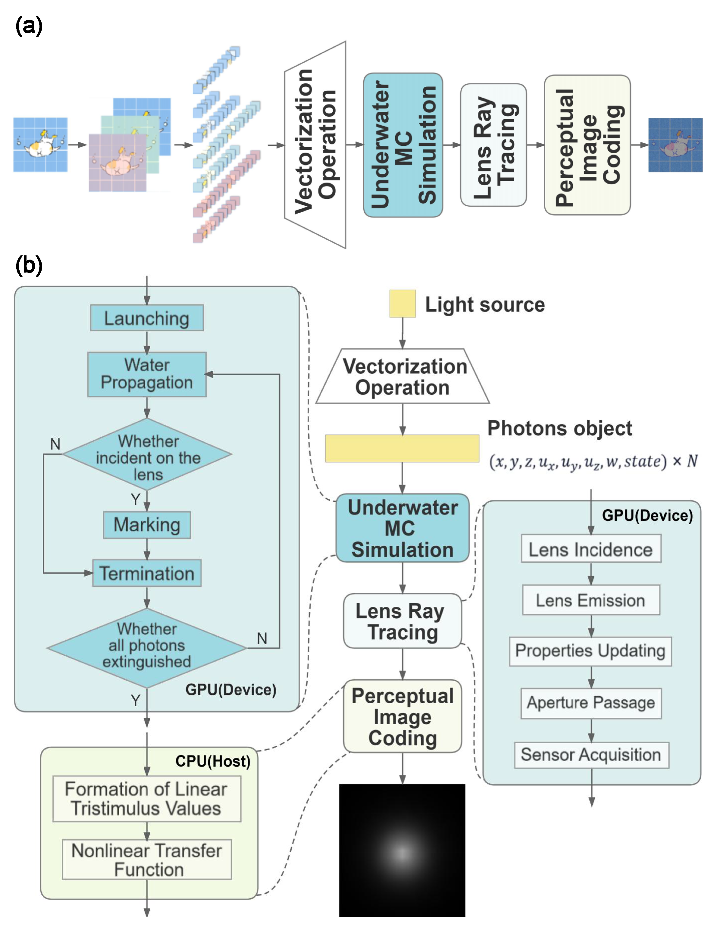
Figure 1 provides an overview of the critical steps to construct this model utilizing parallel MC simulation for the optical imaging model of luminescent objects in deep-sea scenarios. Specifically, this optical imaging model uses the input image to represent luminescent objects, and since the Bayer filter of the image sensor includes red, green, and blue, during the simulation process shown in Figure 1a, we treat each pixel in the channels of the image as an individual point light source. These point light sources emit the respective quantities of red-, green-, and blue-wavelength photons based on the value ratios of the corresponding pixels. Each photon possesses eight attributes encompassing coordinates , direction cosines , weight w, and , denoting survival status. We set a photon quantity threshold before initialization based on the device’s video memory capacity. Afterwards, we group point light sources into propagation batches under this threshold, initializing the photons emitted by all light sources within each batch on the CPU according to Equation (3). Each photon’s position is initialized to with a unit weight w. The initial direction of movement is calculated based on the light source’s divergence angle and angular intensity distribution. As shown in Figure 1b, the eight attributes of these photons are stored in the corresponding order as eight equally sized one-dimensional arrays in NumPy array format [46] and packaged into a ‘’ object. In underwater MC simulation, the equations mentioned in Section 2, Equations (4)–(7), are vectorized, enabling the processing of entire batches of photons at each computation step. For example, variables and are not scalar but NumPy arrays with dimensions corresponding to the attributes of the ‘’ object. Leveraging this vec operation based on the NumPy array facilitates the emission and tracking of an entire batch of photons simultaneously. This eliminates the need for explicit loops for each photon within the program, thereby enhancing code efficiency. Expanding on this approach, we utilize CuPy [38] for interaction between CPU and GPU. Most CuPy array manipulations are closely similar to those of NumPy [47], which maintains consistency and simplicity of the code by preserving the structure of the original NumPy-based code. Concurrently, CuPy allows computations to be executed on the GPU, so as to improve computational speed. The data of the initialized ‘’ object are subsequently transferred from memory to video memory, taking advantage of the GPU’s parallel processing capabilities, which expedites the speed of the MC simulation for underwater light propagation and the ray-tracing for the lens convergence process. Specifically, the GPU can handle many more mathematical calculations simultaneously with greater efficiency due to its highly parallel architecture, this significantly reduces the time requirement for each simulation step. For example, the computation of photons’ propagation direction updates and tracing the photons’ interaction with lenses involve numerous trigonometric and arithmetic operations. These processes can benefit greatly from the GPU’s capacity to handle many operations in parallel.

Figure 1.
An overview of vec operation combined with GPU acceleration for the MC simulation of this model, encompassing photon batch vec operation, GPU parallel computing for photon tracing, and image coding. (a) The simulation for a point source. (b) Using an image to represent a luminescent object.
As illustrated by Figure 1b, during the underwater propagation process, within this batch of photons in the ‘’ object, certain photons may become extinguished due to factors such as moving beyond the boundary of the water medium or having weights below a threshold. In order to monitor the survival status of photons during the underwater MC simulation, the one-dimensional Boolean array is employed to record survival status information, where ‘false’ indicates that the photon was extinguished, and ‘true’ indicates that the photon is still active. In the termination operation, this attribute is employed as a mask to filter and retain only the data in other attributes that correspond to positions in the attribute where the status is ‘true.’ For example, if the attribute array at position i is ‘false’, it signifies that the photon at position i was extinguished, and consequently, the data at the i position of the eight attributes of the ‘’ object would be cleared. Throughout each iteration in the MC simulation for propagation in water, the vec operation described above is employed to update the attributes of each photon in the ‘’ object, mark photons that intersect with the lens, and promptly clear extinguished photons to free unnecessary video memory usage. In the subsequent stage, the convergence process of marked photons through the lens is traced and the acquired photon data from the sensor plane are recorded. During this process, the GPU’s parallel processing capabilities expedite tracing photon paths through the lens and reducing simulation time for photon convergence. Once the entire MC simulation for the underwater imaging process is complete, the recorded data are transferred back to the memory from the video memory. Ultimately, quantization and coding are applied to the sensor-recorded data to visualize the simulation results.
By utilizing the vec operation to handle multiple data points simultaneously through its array-based processing capabilities, and combining GPU parallel acceleration, the simulation speed is further improved. These approaches enable this model to push the computational resource utilization efficiency of MC simulation to a new level.
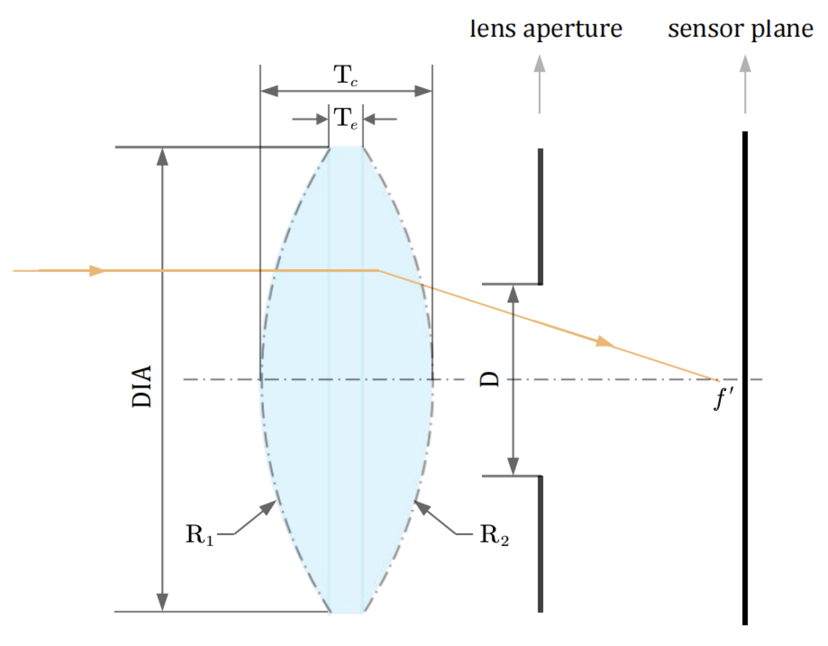
In our imaging system, as shown in Figure 2, we position an aperture diaphragm and the sensor behind the lens. Due to the simple and regular geometrical shape of the lens, implicit shape-based MC techniques can enhance computational speed to a certain extent [48]. Considering the sensitivity of light propagation to local curvature at the boundary, as shown in Figure 3, we define implicit shape parameters for the lens in three dimensions, encompassing the outer diameter , curvature radius , center thickness , and edge thickness , and the entrance pupil diameter for the purpose of using specific equations to describe the lens precisely. is the ratio of the entrance pupil diameter () to the focal length (f) of the lens, which is defined as the relative aperture of the lens. Additionally, an analytical solution is employed to trace the path of photons passing through the lens boundary. By solving quadratic simultaneous equations composed of the incident light’s linear parameter equation and the lens’s double-sided spherical equation, we determine the intersection points of the incident light and the lens boundary. The specific procedure is as follows.
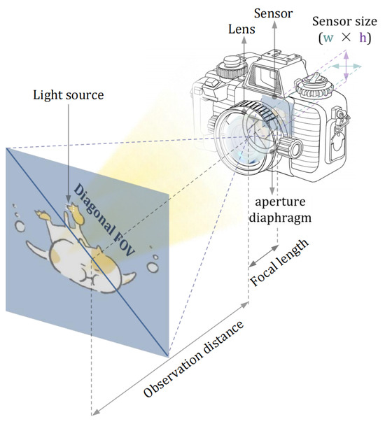
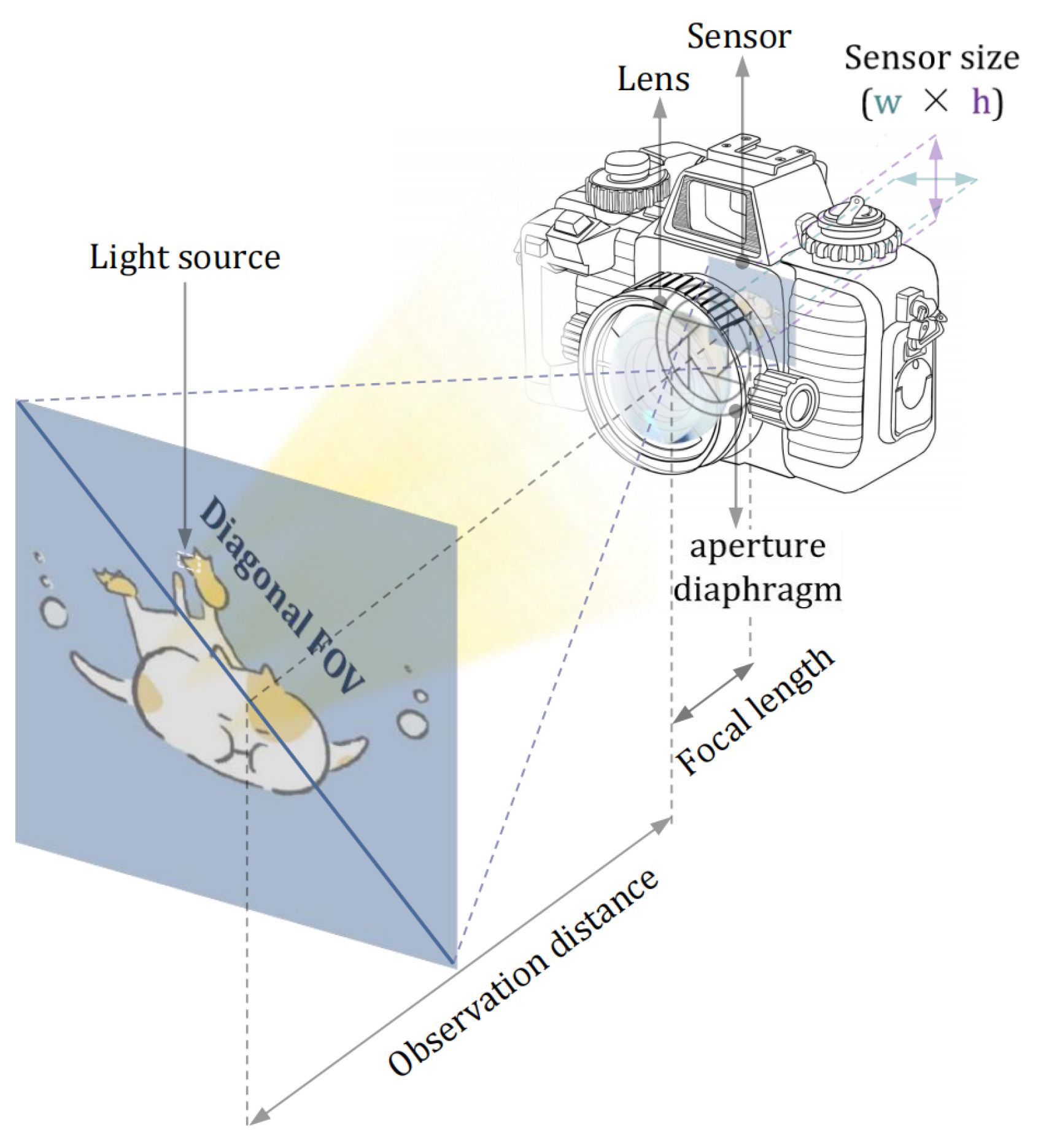
Figure 2.
Schematic illustration of the deep-sea single-lens imaging system for luminescent objects.
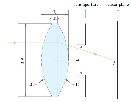
Figure 3.
Two-dimensional schematic of camera imaging system.
In each step of the photon packet transmission process, the photon’s position is constantly traced, and the geometric relationship between the photon’s position and the double-convex lens interface is examined to find if it has intersected the lens boundary within the step size.
The lens center position at and the position of the lens’s upper and lower surfaces’ spherical centers and can be expressed as
The equation of the lens’s double-sided spherical center is
When the photon passes through the lens at a specific step with known initial position coordinates and the directional vector , it intersects the lens’s spherical surface at a certain point . As a result, the incident light’s linear parameter equation can be expressed using , , :
where t is the distance which the light ray has to travel to hit the lens’s spherical surface.
The intersection point of the incident light ray with the lens surface must satisfy both the parameterized equation for the incident light ray and the lens’s spherical equation. By substituting the parameterized equation for the incident light ray into the lens’s spherical equation:
Solving this quadratic equation yields the unknown parameter t:
where and are the two solutions for the unknown parameter t, substituting them into Equation (10) the coordinates of the two intersection points of the incident light ray with the lens’s spherical surface can be derived. The point closest to the photon’s position will be chosen as the intersection point .
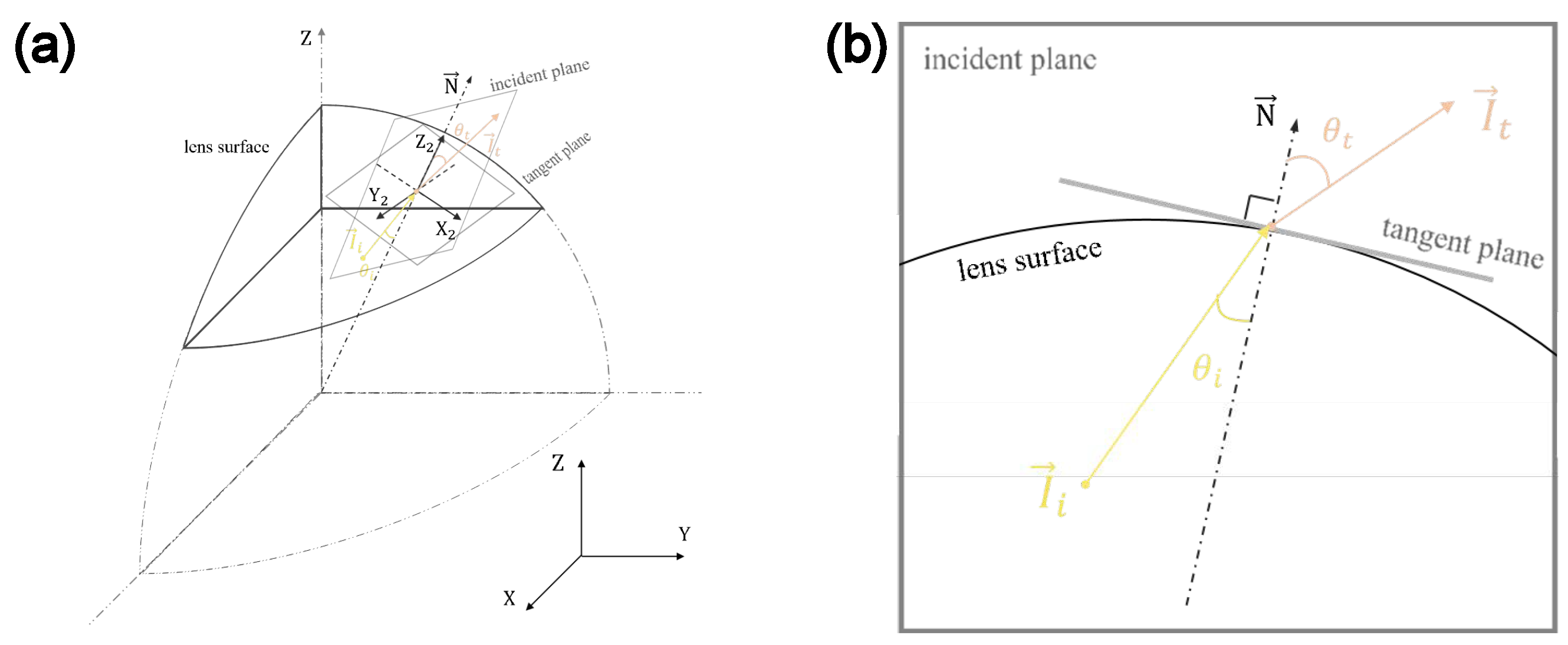
The underwater photon propagation model utilizes a right-handed Cartesian coordinate system with a standard orthogonal basis in three-dimensional space to track photon movements. However, the normal vector to the tangent plane of the lens’s curved boundary does not align with the -axis of the Cartesian coordinate system used in the underwater photon transport model, and it needs to be transformed into a local coordinate system whose -axis matches with the normal to the tangent. Subsequently, a local coordinate system is constructed at the intersection point of each incident photon’s direction vector with the lens boundary. In the local coordinate system , the -axis is tangential to the normal vector of the lens surface at the intersection point, with the positive direction of the local forming an acute angle with the positive direction of the Cartesian coordinate system’s -axis. The vector is orthogonal to the incident plane, and the local coordinate system’s -axis is tangential to and aligned in the same direction. The orientation of the local coordinate system’s -axis is defined by the cross product of and :. As an example of a ray emerging from the lens, the construction schematic of the local coordinate system is shown in Figure 4.
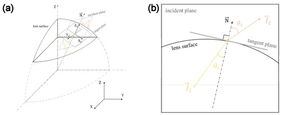
Figure 4.
Schematic diagram of space ray tracing method based on change of basis. (a) Refraction in right-handed Cartesian coordinate system with standard orthogonal basis in three-dimensional space. (b) Refraction in local two-dimensional section of the incident plane.
The system takes the normal vector at the intersection point as the -axis and defines the incidence plane as the plane. Transformation from the Cartesian coordinate system to the local coordinate system is represented by the rotation matrix :
A change of basis is applied to transform the representation of the incident light direction vector and the normal vector of the lens boundary at the intersection point from the Cartesian coordinate system to the local coordinate system. The incident light direction vector is thus expressed in the rotated coordinate system as
The angle of refraction can be assessed from Snell’s law:
and the refracted light direction vector is calculated in the local coordinate system.
The refracted light direction vector expressed in the Cartesian coordinate system is then obtained by multiplying with the inverse of matrix :
As the intensity distribution of each photon’s contribution to the image generated on the sensor placed behind the lens depends on the path through the lens, the Fresnel reflectance is used to adjust the weights of photons during inter-medium transmission:
where is the angle of incidence and is the angle of refraction.
Then, we set the sensor size of the imaging system and further divide it into pixel arrays using a specific sampling grid. Each pixel accumulates the quantity and energy of acquired photons of red, green, and blue light. Subsequently, the spatial distribution of the light intensity across pixel arrays is quantified, resulting in linear R, G, and B tristimulus values. To simulate the nonlinear transfer function of the imaging system, a perceptually uniform (PU) coding scheme [49] is implemented to process the tristimulus signals of each pixel. The normalized energy values of red, green, and blue photons at each pixel grid point on the sensor plane are encoded using the A-law algorithm, as shown in Figure 5, thereby adjusting the relative luminance. Finally, the relative luminance of the pixel grids corresponding to red, green, and blue photons is remapped back into the range of 0 to 255, resulting in the acquisition of numerical data for the red, green, and blue channels of the image, yielding the components of the image. By employing these approaches, we can not only generate images of deep-sea luminescent objects captured at different observation positions and using lenses with varying focal lengths and FOVs, but at the same time, we preserve the spatial resolution of the imaging system.
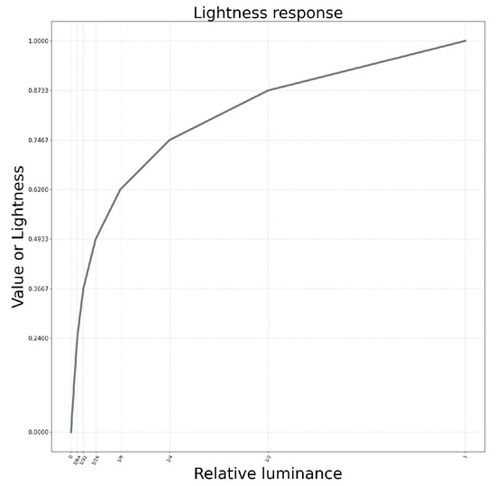
Figure 5.
The tristimulus signals’ value are encoded with PU encoding.
4. Simulation Results
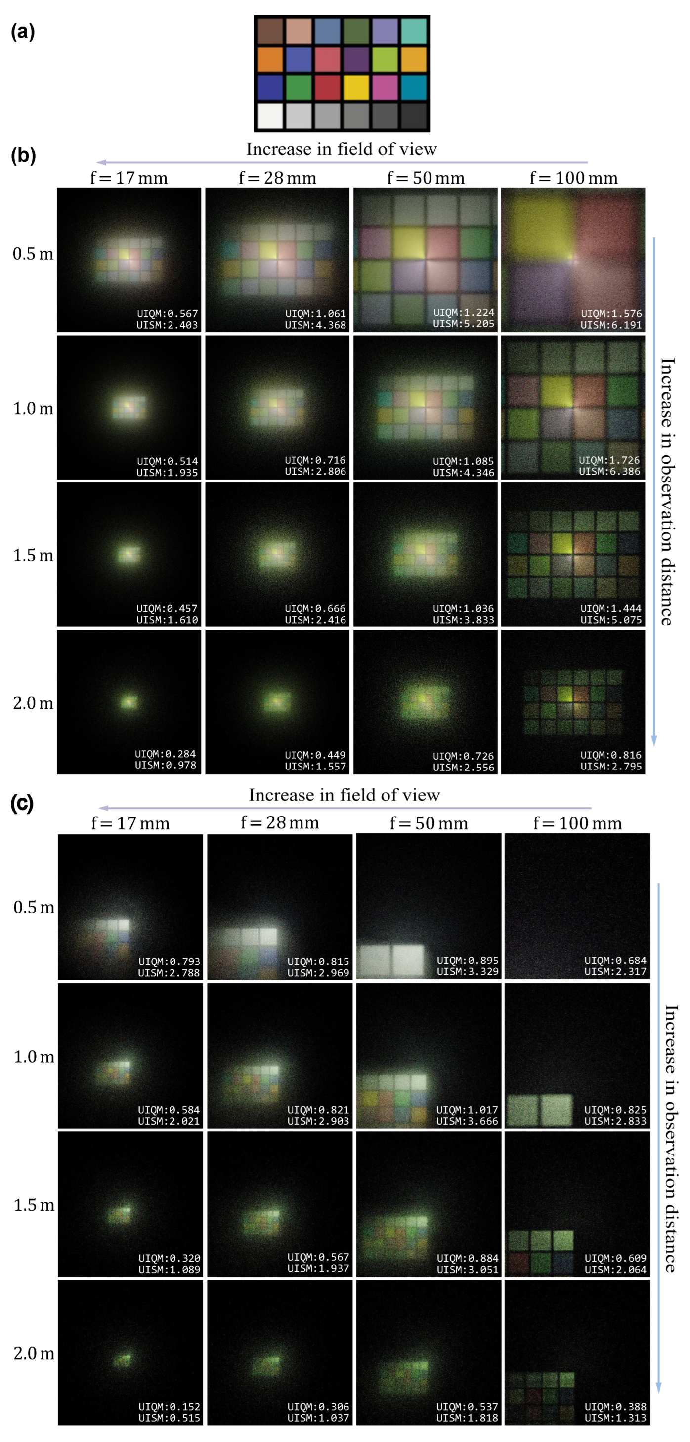
In order to prove that the model is viable, four experiments are set with a sensor of 30 30 and the relative aperture being set to , but each experiment utilizes double-convex lenses made of BK7 glass with different focal lengths f, at 17 , 28 , 50 , and 100 , respectively. These lenses provide diverse FOVs, including wide-angle (), moderately wide-angle (), medium perspective (), and narrow-angle (). A grid density of is used for sampling in the image quantization. For the MC simulation, the water spectrum data of the Tuandao Cape Harbour obtained by our laboratory are used. And the Henyey–Greenstein phase function [43] with an anisotropy factor of 0.924 is applied in the MC simulations for underwater light propagation. The optical properties of Tuandao Cape Harbour’s water and glass mediums are given in Table 1, corresponding to the red, green, and blue wavelengths. We select observation distances of 0.5 , 1 , 1.5 , and 2 , which correspond to approximately 1 to 4 attenuation lengths in the Tuandao Cape Harbour water. As shown in Figure 6a, a ColorChecker chart with 198 × 294 pixels is used to simulate an underwater luminescent object, which corresponds to a physical size of 0.198 0.294 in the simulation. Two distinct scenarios are simulated: one with the luminescent object on the optical axis, with the result as shown in Figure 6b; and the other with the luminescent object far from the optical axis, with the result as shown in Figure 6c.

Table 1.
Absorption coefficient (), attenuation coefficient (), refractive index of Tuandao Cape Harbour water () [50], and refractive index of glass ( [51] values used in simulation model of optical imaging at three different wavelengths ().
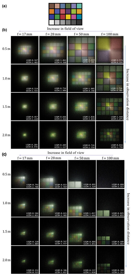
Figure 6.
The images utilized for experiments and those produced by this model. (a) The ColorChecker chart. (b) Images of the ColorChecker chart generated on the optical axis. (c) The ColorChecker chart off the optical axis relative to the position in (b).
Assessing the efficiency of time–cost optimization relies on three primary metrics: simulation time measured in milliseconds; simulation speed calculated as the total number of time steps divided by the simulation time; and lastly, speedup, which is articulated as follows:
In each case, approximately photons are traced. We measure the average simulation speeds across different computing devices for the experiment involving the 50 focal length lens which images the luminescent object positioned on the optical axis. The experimental results shown in Figure 7 indicate that at different detection distances, and using lenses with different focal lengths, our approach demonstrates three orders of magnitude enhancement across various computing devices. Under uniform conditions, the CPU attains an average simulation speed of 1.91 . Upon vec operations without GPU acceleration, the average simulation speed escalates to 2100 . The use of GPU acceleration on the NVIDIA GeForce RTX 4090 device alongside an i9-13900k processor delivers peak performance, with a maximum speed of 7074 . The average acceleration by harnessing the vec operation and employing GPU parallel acceleration, reporting a .
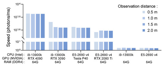
Figure 7.
Average simulation speed on different computing devices.
Additionally, we conducted an experiment using water from a fire hydrant, which possesses distinct water spectrum data from those of the Tuandao Cape Harbour. The optical properties of fire hydrant water and glass mediums are given in Table 2, corresponding to the red, green, and blue wavelengths. This experiment serves to explore the effects of different water optical properties on the simulation outcomes. As shown in Figure 8, the results of this experiment are analyzed in comparison with those obtained using the Tuandao Cape Harbour water, providing insights into the influence of water optical properties on underwater optical imaging simulations.
Table 2.
Absorption coefficient (), attenuation coefficient (), refractive index of fire hydrant water () [50], and refractive index of glass ( [51] values used in simulation model of optical imaging at three different wavelengths ().
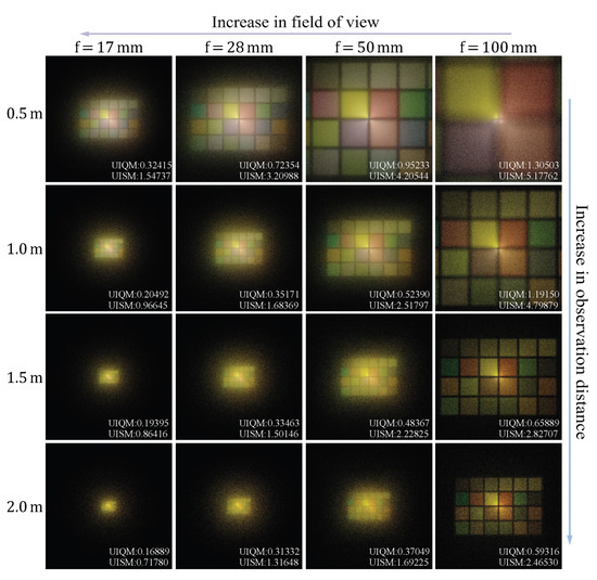
Figure 8.
Comparison results of underwater optical imaging simulation using fire hydrant water.
5. Discussion
The images generated in the experiments are quantitatively evaluated using the underwater image quality measurement (UIQM) and underwater image sharpness measurement (UISM) [52]. UIQM comprises three attribute measures: the underwater image colorfulness measure (UICM), underwater image sharpness measure (UISM), and underwater image contrast measure (UIConM). While evaluating colorfulness, UICM considers bluish or greenish tones and the reduction in color saturation in underwater images, by integrating opposing chrominance components, and . Statistical methods such as asymmetric alpha-trim [53] are applied to compute the colorfulness parameters and , further combined with second-order variances and via weighted aggregation to yield the overall colorfulness metric. Sharpness assessment employs Sobel edge detection and the enhanced measure estimation (EME) approach [54]. The EME approach calculates the Weber contrast entropy [55] within image blocks. These values are then averaged and weighted according to the visual responses of RGB channels to derive UISM. Under consideration of contrast reduction due to back scattering, contrast evaluation utilizes Michelson contrast [55] and the operation [56] to compute contrast entropy within blocks. This is followed by the log-AMEE measure, which is used to result in UIConM. Ultimately, these three metrics are linearly weighted to derive UIQM, which comprehensively evaluates the quality of underwater images based on the parameters of color, sharpness, and contrast.
As shown in Figure 6b,c and Figure 8, the images generated by this model exhibit characteristics that are similar to those images captured by underwater cameras in deep-sea scenarios. They display brightness in the center, darkness in the surroundings, lower contrast, reduced sharpness, and color distortion in perception. For the Tuandao Cape Harbor water, the red-wavelength light has the highest absorption coefficient, resulting in the most severe energy attenuation during underwater propagation. In contrast, the wavelength of the green light experiences comparatively lower absorption and attenuation. Consequently, these images exhibit a greenish tone. Conversely, under the simulated conditions of water from the fire hydrant, blue light possesses the highest absorption coefficient; this leads to the most pronounced energy attenuation during its propagation through water; while the absorption coefficient of red light is comparatively lower, resulting in a slower overall energy attenuation in the red channel. Consequently, under fire hydrant water conditions, the image’s overall hue tends to exhibit a yellow–green tone. Under the same lens configuration, the difficulty of identifying the ColorChecker chart increases progressively as the underwater observation distance increases. This trend is also reflected in the UIQM and UISM scores, which decrease with increasing distance.
The simulated results of the ColorChecker chart on the optical axis are shown in Figure 6b and Figure 8. At the same observation distance, using long-focus lenses with a smaller FOV allows for more precise focusing on the finer details of the target object. This can restrict the view to a smaller volume of the camera’s viewing frustum and filter out the large-angle scattered portions from non-target areas. The acquired underwater images obtain higher UIQM and UISM scores and exhibit better detail and edge clarity. On the other hand, short-focus lenses provide a wider FOV, allowing them to capture the same size underwater area at a closer observation distance than long-focus lenses, thus reducing the length of the water transmission path that degrades underwater imaging quality. In the second scenario, the ColorChecker chart is placed far away from the optical axis, and the results presented in Figure 6c show that the lens–sensor mating format in the simulations causes vignetting in the zoom range. The area near the edge displays a lower contrast and appears more blurred.
6. Conclusions
In conclusion, we propose an optical imaging model for underwater luminescent objects in deep-sea scenarios based on the MC method. The computational speed of MC simulation is expedited as we leverage the vec operation and harness GPU parallel acceleration through the CuPy library. Using analytically defined geometry, we establish a double-convex lens model in a water medium, and then, use forward ray tracing for the underwater imaging process. Finally, quantization and coding are performed to generate imaging results. Utilizing the ColorChecker chart to represent an underwater luminescent object demonstrates that the model can simulate imaging in deep-sea scenarios with various observation positions and imaging device parameters, which include the sensor size, lens focal length, FOV, and relative aperture. Through simulations in different water environments, we illustrate the model’s capability to adapt to varying conditions and its potential for improving underwater imaging systems.
Our model paves the way for more efficient design and optimization of underwater optical imaging systems, particularly in deep-sea environments, by providing a detailed understanding of the interplay between light scattering, absorption properties, and system configuration. In future research, we aim to extend this model to explore more complex imaging systems and scenarios, providing essential simulation support for the configuration of underwater optical imaging technologies, such as the range-gated technique, laser synchronous scanning technique, and streak tube imaging lidar.
Author Contributions
Methodology, Q.H.; simulation experiments, Q.H.; supervision, M.S., B.Z. and M.F.; writing—original draft, Q.H.; review and editing, M.S. All authors have read and agreed to the published version of the manuscript.
Funding
This work was financially supported by the Provincial Natural Science Foundation of Shandong [ZR2021QD089], National Key Research and Development Program of China [2022YFD2401304], and Fundamental Research Funds for the Central Universities [202113040].
Data Availability Statement
The data presented in this study are available upon request from the corresponding author. Due to privacy, the data cannot be made public.
Conflicts of Interest
The authors declare no conflicts of interest.
Abbreviations
The following abbreviations are used in this manuscript:
| MC | Monte Carlo |
| FOV | Field of view |
| vec | Vectorization |
References
- Loureiro, G.; Dias, A.; Almeida, J.; Martins, A.; Hong, S.; Silva, E. A Survey of Seafloor Characterization and Mapping Techniques. Remote Sens. 2024, 16, 1163. [Google Scholar] [CrossRef]
- Sibley, E.C.; Elsdon, T.S.; Marnane, M.J.; Madgett, A.S.; Harvey, E.S.; Cornulier, T.; Driessen, D.; Fernandes, P.G. Sound sees more: A comparison of imaging sonars and optical cameras for estimating fish densities at artificial reefs. Fish. Res. 2023, 264, 106720. [Google Scholar] [CrossRef]
- Luo, J.; Han, Y.; Fan, L. Underwater acoustic target tracking: A review. Sensors 2018, 18, 112. [Google Scholar] [CrossRef] [PubMed]
- Kumar, N.; Mitra, U.; Narayanan, S.S. Robust object classification in underwater sidescan sonar images by using reliability-aware fusion of shadow features. IEEE J. Ocean. Eng. 2014, 40, 592–606. [Google Scholar] [CrossRef]
- Wachowski, N.; Azimi-Sadjadi, M.R. A new synthetic aperture sonar processing method using coherence analysis. IEEE J. Ocean. Eng. 2011, 36, 665–678. [Google Scholar] [CrossRef]
- Yang, P. An imaging algorithm for high-resolution imaging sonar system. Multimed. Tools Appl. 2023, 83, 31957–31973. [Google Scholar] [CrossRef]
- Zhang, X.; Yang, P.; Wang, Y.; Shen, W.; Yang, J.; Wang, J.; Ye, K.; Zhou, M.; Sun, H. A Novel Multireceiver SAS RD Processor. IEEE Trans. Geosci. Remote Sens. 2024, 62, 4203611. [Google Scholar] [CrossRef]
- Chinicz, R.; Diamant, R. A Statistical Evaluation of the Connection between Underwater Optical and Acoustic Images. Remote Sens. 2024, 16, 689. [Google Scholar] [CrossRef]
- Abu, A.; Diamant, R. Feature set for classification of man-made underwater objects in optical and SAS data. IEEE Sens. J. 2022, 22, 6027–6041. [Google Scholar] [CrossRef]
- Zhang, X.; Yang, P.; Wang, Y.; Shen, W.; Yang, J.; Ye, K.; Zhou, M.; Sun, H. Lbf-based cs algorithm for multireceiver sas. IEEE Geosci. Remote Sens. Lett. 2024, 21, 1502505. [Google Scholar] [CrossRef]
- Xi, Z.; Zhao, J.; Zhu, W. Side-Scan Sonar Image Simulation Considering Imaging Mechanism and Marine Environment for Zero-Shot Shipwreck Detection. IEEE Trans. Geosci. Remote Sens. 2023, 61, 1–13. [Google Scholar] [CrossRef]
- Kunz, C.; Singh, H. Map building fusing acoustic and visual information using autonomous underwater vehicles. J. Field Robot. 2013, 30, 763–783. [Google Scholar] [CrossRef]
- Lagudi, A.; Bianco, G.; Muzzupappa, M.; Bruno, F. An alignment method for the integration of underwater 3D data captured by a stereovision system and an acoustic camera. Sensors 2016, 16, 536. [Google Scholar] [CrossRef] [PubMed]
- Kim, H.G.; Seo, J.; Kim, S.M. Underwater optical-sonar image fusion systems. Sensors 2022, 22, 8445. [Google Scholar] [CrossRef] [PubMed]
- Lu, H.; Li, Y.; Zhang, Y.; Chen, M.; Serikawa, S.; Kim, H. Underwater optical image processing: A comprehensive review. Mob. Netw. Appl. 2017, 22, 1204–1211. [Google Scholar] [CrossRef]
- Mariani, P.; Quincoces, I.; Haugholt, K.H.; Chardard, Y.; Visser, A.W.; Yates, C.; Piccinno, G.; Reali, G.; Risholm, P.; Thielemann, J.T. Range-gated imaging system for underwater monitoring in ocean environment. Sustainability 2018, 11, 162. [Google Scholar] [CrossRef]
- Wu, H.; Zhao, M.; Xu, W. Underwater de-scattering imaging by laser field synchronous scanning. Opt. Lasers Eng. 2020, 126, 105871. [Google Scholar] [CrossRef]
- Gao, J.; Sun, J.; Wei, J.; Wang, Q. Research of underwater target detection using a slit streak tube imaging lidar. In Proceedings of the 2011 Academic International Symposium on Optoelectronics and Microelectronics Technology, Harbin, China, 12–16 October 2011; pp. 240–243. [Google Scholar]
- McGlamery, B. A computer model for underwater camera systems. In Proceedings of the Ocean Optics VI; SPIE; Monterey, CA, USA, 1980; Volume 208, pp. 221–231. [Google Scholar]
- Jaffe, J.S. Computer modeling and the design of optimal underwater imaging systems. IEEE J. Ocean. Eng. 1990, 15, 101–111. [Google Scholar] [CrossRef]
- Wang, Y.; Song, W.; Fortino, G.; Qi, L.Z.; Zhang, W.; Liotta, A. An experimental-based review of image enhancement and image restoration methods for underwater imaging. IEEE Access 2019, 7, 140233–140251. [Google Scholar] [CrossRef]
- Liu, Y.; Xu, H.; Shang, D.; Li, C.; Quan, X. An underwater image enhancement method for different illumination conditions based on color tone correction and fusion-based descattering. Sensors 2019, 19, 5567. [Google Scholar] [CrossRef]
- Zhang, Y.; Jiang, Q.; Liu, P.; Gao, S.; Pan, X.; Zhang, C. Underwater Image Enhancement Using Deep Transfer Learning Based on a Color Restoration Model. IEEE J. Ocean. Eng. 2023, 48, 489–514. [Google Scholar] [CrossRef]
- Akkaynak, D.; Treibitz, T. Sea-thru: A method for removing water from underwater images. In Proceedings of the IEEE/CVF Conference on Computer Vision and Pattern Recognition, Long Beach, CA, USA, 15–20 June 2019; pp. 1682–1691. [Google Scholar]
- Mertens, L.E. In-Water Photography: Theory and Practice; John Wiley & Sons: New York, NY, USA, 1970. [Google Scholar]
- Zhu, S.; Guo, E.; Gu, J.; Bai, L.; Han, J. Imaging through unknown scattering media based on physics-informed learning. Photonics Res. 2021, 9, B210–B219. [Google Scholar] [CrossRef]
- Ke, X.; Yang, S.; Sun, Y.; Liang, J.; Pan, X. Underwater blue-green LED communication using a double-layered, curved compound-eye optical system. Opt. Express 2022, 30, 18599–18616. [Google Scholar] [CrossRef] [PubMed]
- Vadakke-Chanat, S.; Shanmugam, P.; Sundarabalan, B. Monte Carlo simulations of the backscattering measurements for associated uncertainty. Opt. Express 2018, 26, 21258–21270. [Google Scholar] [CrossRef] [PubMed]
- Preisendorfer, R.W. Unpolarized Irradiance Reflectances and Glitter Patterns of Random Capillary Waves on Lakes and Seas, by Monte Carlo Simulation; US Department of Commerce, National Oceanic and Atmospheric Administration: Pacific Marine Environmental Laboratory: Seattle, WA, USA, 1985; Volume 63.
- Xu, F.; He, X.; Jin, X.; Cai, W.; Bai, Y.; Wang, D.; Gong, F.; Zhu, Q. Spherical vector radiative transfer model for satellite ocean color remote sensing. Opt. Express 2023, 31, 11192–11212. [Google Scholar] [CrossRef] [PubMed]
- Wang, L.; Jacques, S.L.; Zheng, L. MCML—Monte Carlo modeling of light transport in multi-layered tissues. Comput. Methods Programs Biomed. 1995, 47, 131–146. [Google Scholar] [CrossRef] [PubMed]
- Alerstam, E.; Svensson, T.; Andersson-Engels, S. Parallel computing with graphics processing units for high-speed Monte Carlo simulation of photon migration. J. Biomed. Opt. 2008, 13, 060504. [Google Scholar] [CrossRef] [PubMed]
- Fang, Q.; Yan, S. Graphics processing unit-accelerated mesh-based Monte Carlo photon transport simulations. J. Biomed. Opt. 2019, 24, 115002. [Google Scholar] [CrossRef] [PubMed]
- Ramon, D.; Steinmetz, F.; Jolivet, D.; Compiègne, M.; Frouin, R. Modeling polarized radiative transfer in the ocean-atmosphere system with the GPU-accelerated SMART-G Monte Carlo code. J. Quant. Spectrosc. Radiat. Transf. 2019, 222, 89–107. [Google Scholar] [CrossRef]
- Yang, Y.; Guo, L. Parallel Monte Carlo simulation algorithm for the spectral reflectance and transmittance of the wind-generated bubble layers in the upper ocean using CUDA. Opt. Express 2020, 28, 33538–33555. [Google Scholar] [CrossRef]
- Liao, Y.; Shangguan, M.; Yang, Z.; Lin, Z.; Wang, Y.; Li, S. GPU-Accelerated Monte Carlo Simulation for a Single-Photon Underwater Lidar. Remote Sens. 2023, 15, 5245. [Google Scholar] [CrossRef]
- Du, Z.; Ge, W.; Song, G.; Dai, Y.; Zhang, Y.; Xiong, J.; Jia, B.; Hua, Y.; Ma, D.; Zhang, Z.; et al. Partially pruned DNN coupled with parallel Monte-Carlo algorithm for path loss prediction in underwater wireless optical channels. Opt. Express 2022, 30, 12835–12847. [Google Scholar] [CrossRef] [PubMed]
- Okuta, R.; Unno, Y.; Nishino, D.; Hido, S.; Loomis, C. CuPy: A NumPy-Compatible Library for NVIDIA GPU Calculations. In Proceedings of the Workshop on Machine Learning Systems (LearningSys) in the Thirty-first Annual Conference on Neural Information Processing Systems (NIPS), Long Beach, CA, USA, 4–9 December 2017. [Google Scholar]
- Arvo, J.; Cook, R.L.; Glassner, A.S.; Haines, E.; Hanrahan, P.; Heckbert, P.S.; Kirk, D. Backward ray tracing. Dev. Ray Tracing 1986, 12, 259–263. [Google Scholar]
- Schechner, Y.Y.; Karpel, N. Clear underwater vision. In Proceedings of the 2004 IEEE Computer Society Conference on Computer Vision and Pattern Recognition, Washington, DC, USA, 27 June 2004–2 July 2004; Volume 1, p. I. [Google Scholar]
- Akkaynak, D.; Treibitz, T. A revised underwater image formation model. In Proceedings of the IEEE Conference on Computer Vision and Pattern Recognition, Salt Lake City, UT, USA, 18–23 June 2018; pp. 6723–6732. [Google Scholar]
- Sassaroli, A.; Martelli, F. Equivalence of four Monte Carlo methods for photon migration in turbid media. JOSA A 2012, 29, 2110–2117. [Google Scholar] [CrossRef]
- Henyey, L.G.; Greenstein, J.L. Diffuse radiation in the galaxy. Astrophys. J. 1941, 93, 70–83. [Google Scholar] [CrossRef]
- Kattawar, G.W. A three-parameter analytic phase function for multiple scattering calculations. J. Quant. Spectrosc. Radiat. Transf. 1975, 15, 839–849. [Google Scholar] [CrossRef]
- Haltrin, V.I. One-parameter two-term Henyey-Greenstein phase function for light scattering in seawater. Appl. Opt. 2002, 41, 1022–1028. [Google Scholar] [CrossRef] [PubMed]
- Van Der Walt, S.; Colbert, S.C.; Varoquaux, G. The NumPy array: A structure for efficient numerical computation. Comput. Sci. Eng. 2011, 13, 22–30. [Google Scholar] [CrossRef]
- Tokui, S.; Okuta, R.; Akiba, T.; Niitani, Y.; Ogawa, T.; Saito, S.; Suzuki, S.; Uenishi, K.; Vogel, B.; Yamazaki Vincent, H. Chainer: A deep learning framework for accelerating the research cycle. In Proceedings of the 25th ACM SIGKDD International Conference on Knowledge Discovery & Data Mining, Anchorage, AK, USA, 4–8 August 2019; pp. 2002–2011. [Google Scholar]
- Yuan, Y.; Yan, S.; Fang, Q. Light transport modeling in highly complex tissues using the implicit mesh-based Monte Carlo algorithm. Biomed. Opt. Express 2021, 12, 147–161. [Google Scholar] [CrossRef]
- Poynton, C.A. Rehabilitation of gamma. In Proceedings of the Human Vision and Electronic Imaging III, San Jose, CA, USA, 26–29 January 1998; Volume 3299, pp. 232–249. [Google Scholar]
- Segelstein, D.J. The Complex Refractive Index of Water. Ph.D. Thesis, University of Missouri, Kansas City, MO, USA, 1981. [Google Scholar]
- Englert, M.; Hartmann, P.; Reichel, S. Optical glass: Refractive index change with wavelength and temperature. In Proceedings of the Optical Modelling and Design III, Stockholm, Sweden, 19–22 May 2014; Volume 9131, pp. 125–138. [Google Scholar]
- Panetta, K.; Gao, C.; Agaian, S. Human-visual-system-inspired underwater image quality measures. IEEE J. Ocean. Eng. 2015, 41, 541–551. [Google Scholar] [CrossRef]
- Bednar, J.; Watt, T. Alpha-trimmed means and their relationship to median filters. IEEE Trans. Acoust. Speech, Signal Process. 1984, 32, 145–153. [Google Scholar] [CrossRef]
- Panetta, K.; Samani, A.; Agaian, S. Choosing the optimal spatial domain measure of enhancement for mammogram images. J. Biomed. Imaging 2014, 2014, 937849. [Google Scholar] [CrossRef] [PubMed]
- Peli, E. Contrast in complex images. JOSA A 1990, 7, 2032–2040. [Google Scholar] [CrossRef] [PubMed]
- Panetta, K.; Agaian, S.; Zhou, Y.; Wharton, E.J. Parameterized logarithmic framework for image enhancement. IEEE Trans. Syst. Man, Cybern. Part B Cybern. 2010, 41, 460–473. [Google Scholar] [CrossRef] [PubMed]


Disclaimer/Publisher’s Note: The statements, opinions and data contained in all publications are solely those of the individual author(s) and contributor(s) and not of MDPI and/or the editor(s). MDPI and/or the editor(s) disclaim responsibility for any injury to people or property resulting from any ideas, methods, instructions or products referred to in the content. |
© 2024 by the authors. Licensee MDPI, Basel, Switzerland. This article is an open access article distributed under the terms and conditions of the Creative Commons Attribution (CC BY) license (https://creativecommons.org/licenses/by/4.0/).