CVTNet: A Fusion of Convolutional Neural Networks and Vision Transformer for Wetland Mapping Using Sentinel-1 and Sentinel-2 Satellite Data

Abstract

Wetland mapping is a critical component of environmental monitoring, requiring advanced techniques to accurately represent the complex land cover patterns and subtle class differences innate in these ecosystems. This study aims to address these challenges by proposing CVTNet, a novel deep learning (DL) model that integrates convolutional neural networks (CNNs) and vision transformer (ViT) architectures. CVTNet uses channel attention (CA) and spatial attention (SA) mechanisms to enhance feature extraction from Sentinel-1 (S1) and Sentinel-2 (S2) satellite data. The primary goal of this model is to achieve a balanced trade-off between Precision and Recall, which is essential for accurate wetland mapping. The class-specific analysis demonstrated CVTNet’s proficiency across diverse classes, including pasture, shrubland, urban, bog, fen, and water. Comparative analysis showed that CVTNet outperforms contemporary algorithms such as Random Forest (RF), ViT, multi-layer perceptron mixer (MLP-mixer), and hybrid spectral net (HybridSN) classifiers. Additionally, the attention mechanism (AM) analysis and sensitivity analysis highlighted the crucial role of CA, SA, and ViT in focusing the model’s attention on critical regions, thereby improving the mapping of wetland regions. Despite challenges at class boundaries, particularly between bog and fen, and misclassifications of swamp pixels, CVTNet presents a solution for wetland mapping.

1. Introduction

Wetlands, characterized by their unique intersection of freshwater and saltwater environments and identified by perpetually wet soils due to frequent flooding [1], play a vital role in the environment through essential biogeochemical and hydrological processes [2]. These ecosystems, dominated by emergent plants, shrubs, and woodland vegetation, offer a myriad of benefits, including flood control, erosion prevention, nutrient provision, recreational opportunities, and aesthetic value [3]. Moreover, wetlands contribute to crucial environmental services such as protection from flood and storm damage, enhancement of water quality, reduction of greenhouse gases, shoreline stabilization, and support for diverse fish and wildlife species [4]. Despite their significance, 20th-century wetlands have faced substantial damage from industrialization, climate change, and pollution [5]. Given these challenges and the critical importance of wetlands, creating precise maps detailing their location and composition becomes paramount [6].

Accurate wetland maps serve as vital resources for understanding the spatial distribution, ecosystem functions, and temporal changes within these invaluable environments [7]. Traditional mapping methods, such as surveying, prove laborious and expensive, particularly given the remote, expansive, and seasonally dynamic characteristics of many wetland ecosystems [4]. Fortunately, remote sensing emerged as a cost-effective and efficient alternative approach, providing ecological data crucial for describing and monitoring wetland ecosystems. Satellite-based Earth monitoring, utilizing optical and radar systems, has evolved into a valuable tool for wetland mapping. The European Space Agency’s (ESA) Copernicus program, specifically the Sentinel-1 (S1) and Sentinel-2 (S2) missions, presents a unique opportunity to improve wetland mapping accuracy. These missions provide free access to high-resolution S1 and S2 data, offering exceptional spatial and temporal resolutions. S1 satellites, equipped with C-band Synthetic Aperture Radar, operate at a 10 m resolution and prove to be effective in detecting water bodies hidden beneath vegetation canopies [8,9]. In parallel, S2 satellites, with a multispectral sensor offering optical data at various resolutions, complement the radar data [10]. Both missions, involving two polar-orbiting satellites, provide relatively frequent revisit times of every five to six days at the equator [11].

Despite significant progress in remote sensing technology, classifying complex and heterogeneous land cover types like wetlands remains a challenging task [12]. The challenge arises from the fact that in highly fragmented landscapes like wetlands, there exist numerous small classes that lack distinct boundaries between them, resulting in heightened variability within the same class and reduced distinguishability between different classes [5]. Moreover, certain classes among these may exhibit highly similar spectral properties thus, complicating their separation and requiring advanced methods for an accurate classification.

A crucial factor in achieving accurate wetland categorization through remote sensing data hinges on the selection of an appropriate classification algorithm [13]. Over the past few years, numerous advanced machine learning (ML) algorithms have been used for the purpose of wetland classification [4,14,15,16,17,18]. Presently, deep learning (DL) algorithms have demonstrated a high level of accuracy in the context of wetland mapping [3]. Deep learning (DL) algorithms, such as convolutional neural networks (CNNs), have shown significant advancements in handling complex datasets due to their ability to extract and learn hierarchical features from raw data automatically [19,20]. Unlike shallow models like Random Forest (RF), which rely on manual feature engineering and are limited by their relatively simplistic structure, DL models can discover complex patterns and relationships within large and heterogeneous datasets [21]. For instance, CNNs excel at identifying spatial hierarchies and local features through convolutional layers. These capabilities are particularly beneficial for tasks such as wetland mapping, where diverse land cover patterns and subtle class differences necessitate sophisticated feature extraction and representation [22]. Empirical studies have demonstrated that DL models often achieve higher accuracy and robustness compared to shallow models in wetland mapping [4,5,12,23].

CNNs, a class of DL models inspired by biological processes, are widely employed for the classification of remote sensing images, consistently achieving high accuracy in complex, high-dimensional scenarios [24,25,26]. Following the emergence of cutting-edge CNN models like AlexNet [27], VGG [28], and ResNet [29], which achieved remarkable performance in the ImageNet image classification challenge, CNN architectures have solidified their position as the dominant and most influential designs for computer vision tasks. Nonetheless, the advent of transformers in the field of natural language processing (NLP) and text processing directed attention toward considering the possible application of these innovative architectures in the vision tasks [30]. The key factor behind the transformers’ achievement of high accuracy is the attention mechanism (AM), which enables the model to assign greater importance to various regions or patches within the image [31]. Recently, attention-based models, such as vision transformers (ViT), swin transformers, etc., have been demonstrated to be effective in several tasks, including some instances of remote sensing image classification [32,33,34]. Previous studies demonstrated the benefits of using both CNNs and transformers by changing the multi-head attention blocks with convolutional layers [35], adding more parallel convolutional layers [36], and using sequential convolutional layers [37]. These approaches can result in capturing local dependencies. Despite these advances in other remote sensing applications, the potential of combining state-of-the-art CNN architectures with transformers in wetland mapping is underrepresented and requires further exploration.

This study introduces a novel deep learning model for wetland mapping using S1 and S2 data. The primary contributions of this study are: (1) using the potential of both CNNs and ViT to develop a novel DL model called CVTNet, which improves feature extraction through channel attention (CA) and spatial attention (SA); (2) evaluating the effects of attention mechanisms (AMs) in CVTNet model using the gradient-weighted class activation mapping (Grad-CAM) algorithm and occlusion sensitivity maps; (3) and assessing the model’s capability at distinguishing wetland class boundaries.

2. Materials and Methods

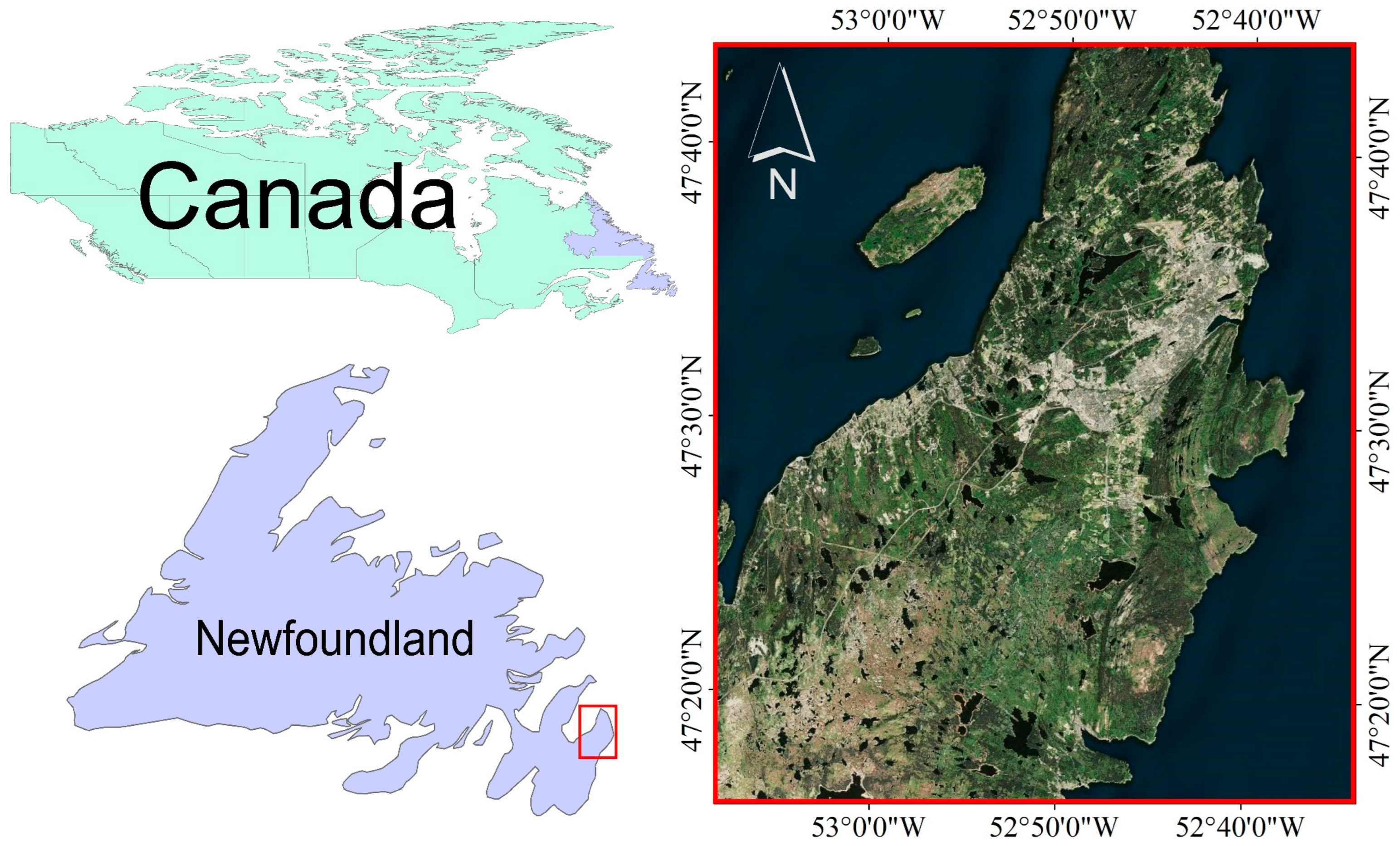
2.1. Study Area

The study area is in Eastern Newfoundland and Labrador, bordered by the Atlantic Ocean (see Figure 1). It covers approximately 1996.631 square kilometers and has a humid continental climate. St. John’s, the largest city’s capital, has around 226,000 residents. The land cover includes diverse wetland types such as bogs, fens, forests, grasslands, marshes, pastures, shrubbery, urban areas, swamps, and water bodies. According to the Canadian Wetland Classification System (CWSC), the primary wetlands here are bogs, marshes, fens, and swamps, with bogs and fens (peatlands) predominant.

2.2. Data

This study used S1 and S2 satellite data from Google Earth Engine (GEE) with a 10 m spatial resolution. The maskS2clouds algorithm [1] filtered S2 data for less than 10% cloud coverage from 15 May to 27 May 2022. S2 satellite data includes three different spatial resolutions: 10 m for visible and near-infrared bands, 20 m for red-edge and shortwave infrared bands, and 60 m for atmospheric correction bands. We selected the 10 and 20 m bands (B2, B3, B4, B5, B6, B7, B8, B8A, B11, B12), resampling the 20 m bands to 10 m for consistency. S1 ground range detected (GRD) data included ${\sigma }_{VV}^0$, ${\sigma }_{VH}^0$, ${\sigma }_{HH}^0$, and ${\sigma }_{HV}^0$. The spatial resolution of S1 data in Interferometric Wide (IW) mode, as obtained from GEE, has a pixel spacing of approximately 10 m, though its spatial resolution is not precisely 10 m due to the nature of radar imaging. Preprocessing involved noise removal, terrain adjustment, and radiometric calibration using the ESA Sentinel toolbox. Both S1 and S2 data were acquired from 15 May to 27 May 2022.

Table 1. The details of spectral bands and backscattering coefficients used in this study.

Data	Spectral Band/Backscattering Coefficients	Date Range	Spatial Resolution
S2	B2, B3, B4, B5, B6, B7, B8, B8A, B11, B12	15 May to 27 May 2022	10 m
S1	${\sigma }_{VV}^0$, ${\sigma }_{VH}^0$, ${\sigma }_{HH}^0$, ${\sigma }_{HV}^0$

shows the details of S1 and S2 data used in this study.

Training and validation datasets, labeled by specialists using GPS and high-resolution imagery, were collected from 2017 to 2019. The training set includes 638 polygons, and the validation set has 249 polygons, each with diverse sizes and classes. These datasets were obtained from different geographic regions to avoid data leakage. Figure 2 indicates the distribution of training and validation sets. Moreover, non-wetland classes such as water, urban, and grass were included to prevent over-classification of wetlands.

Table 2. Details regarding the number of polygons and their corresponding area measurements for each class.

Class	Number of Polygon		Area (km2)
	Training	Validation	Training	Validation
Bog	72	26	1.79	0.55
Fen	80	33	1.11	0.51
Exposed	20	4	0.05	0.02
Forest	72	31	1.41	0.59
Grassland	87	39	0.55	0.34
Marsh	29	20	0.12	0.04
Pasture	30	17	0.85	0.29
Shrub	21	16	0.18	0.13
Swamp	83	33	0.52	0.2
Urban	35	13	1.24	0.29
Water	52	17	1.14	0.36

shows the number of polygons within each class and their respective area measurements in both the training and validation datasets.

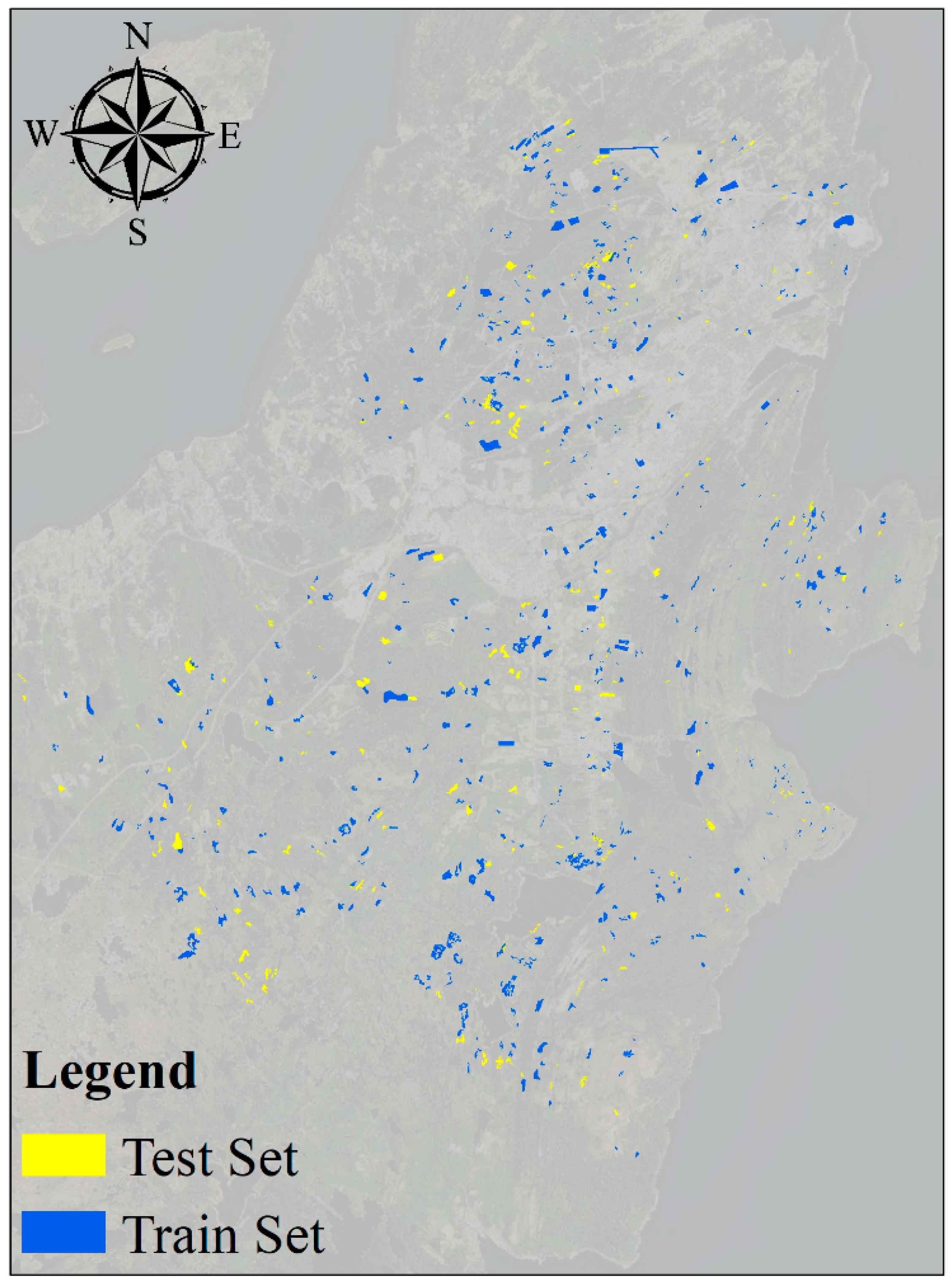
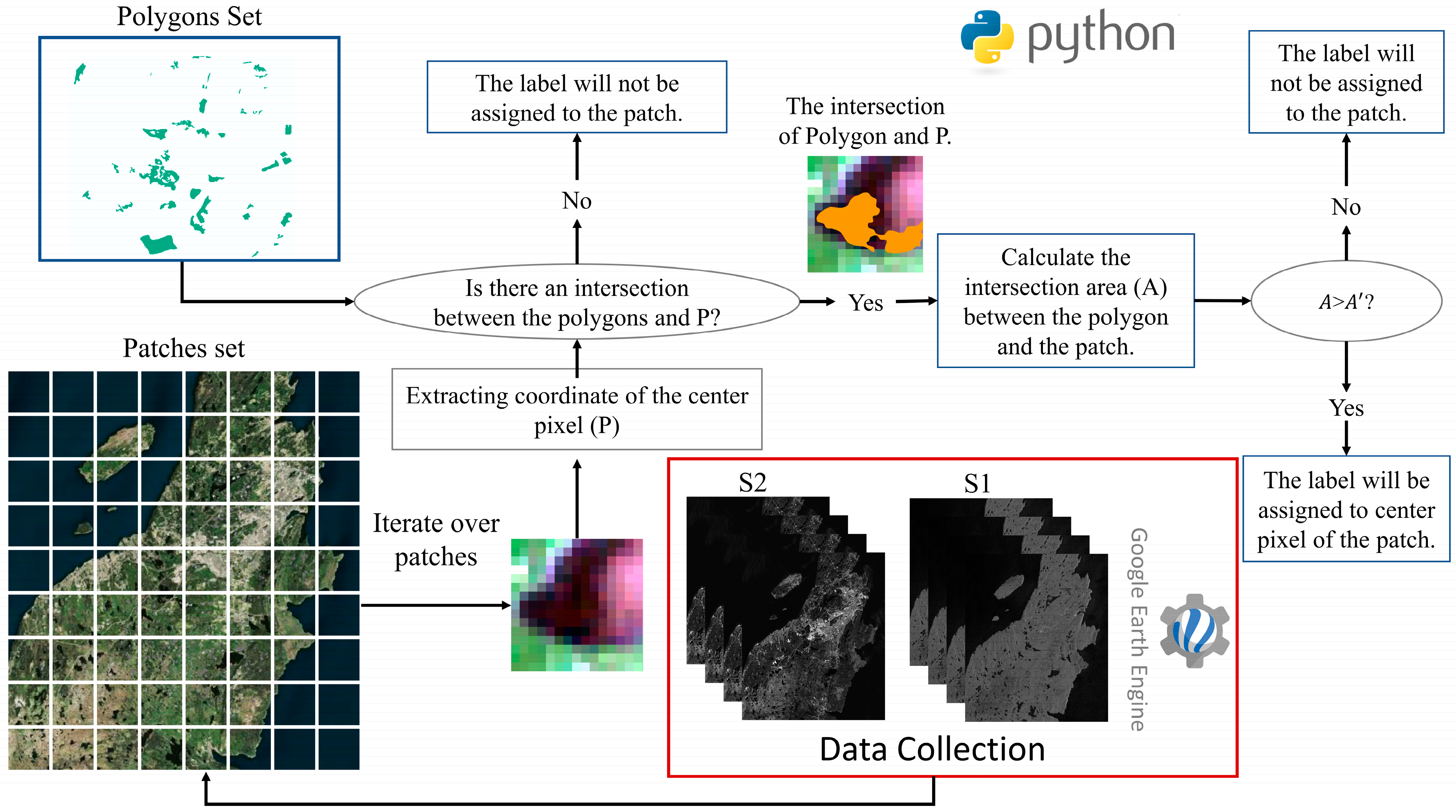
2.3. Data Preparation and Label Assigning

The satellite data employed in this study were represented in a three-dimensional format with dimensions $m\times n\times c$ where $m$ and $n$ are the image’s height and width, respectively, and $c$ is the number of channels. Given the large size of the satellite image, processing it in its entirety proved time-intensive. Consequently, the image was subdivided into multiple patches along both the $x$ and $y$ dimensions, resulting in a new shape of $m^{\prime }\times n^{\prime }\times c$ (where $m^{\prime }$ < $m$ and $n^{\prime }$ < $n$) [4]. To address the challenge of labeling these patches, we adopted a patch-based method, assigning labels to the center of each patch [15], as illustrated in Figure 3.

Initially, S1 data (comprising 4 backscattering bands) and S2 data (comprising 10 spectral bands) for the study area were collected using GEE. These data were then combined along their respective channels, resulting in an image with 14 bands. The 14-band image was subsequently partitioned into multiple patches with a 50% overlay. To determine the optimal patch size, a trial-and-error methodology was employed, experimenting with patch sizes of 8, 12, 15, and 20. These patch sizes were proposed by previous studies for S1 and S2 data [3]. The investigation showed that a patch size of 8 produced optimal results.

Next, the central coordinate of the patch (P) was extracted, and its intersection with a set of training and validation polygons was evaluated. If there was no intersection, the patch remained unlabeled. Conversely, if an intersection occurred between P and the polygon set, the intersection area (A) between the patch and the polygon was calculated.

Subsequently, A was compared with a predefined area value (A’). If A > A’, the label of the polygon was assigned to the patch; otherwise, no label was assigned. Notably, A’ varied based on patch sizes, with values of 400, 900, 1400, and 2500 m² corresponding to patch sizes of 8, 12, 15, and 20, respectively. A’ signified the area covered by a polygon exclusively belonging to a single wetland class. In

Table 3. Number of patches for each class using a patch size of 8.

Class	Number of Patches
	Training	Validation
Bog	1101	349
Fen	679	325
Exposed	36	12
Forest	890	365
Grassland	346	216
Marsh	67	24
Pasture	537	183
Shrubland	116	93
Swamp	313	128
Urban	750	189
Water	708	234

, the number of extracted patches for each class can be observed and each patch is sized at 8.

2.4. Convolutional Neural Network (CNN)

The CNN algorithm is a powerful DL approach that eliminates the necessity for prior feature extraction [38]. A standard CNN comprises three primary layer types: the convolution layer, the pooling layer, and the fully connected layer. The convolution layer, the foundational element in extracting information from preceding layers, uses filters on input data to identify diverse features such as edges, textures, and shapes through learnable parameters [39]. CNNs maintain connections between pixels, preserving spatial information [23]. Equation (1) defines a simple convolution operation involving the input image $I$ and the kernel $K$, where $m$ and $n$ denote the dimensions of $K$ [5]:

$$FeatureMap=I\times Kernel={\displaystyle \sum }_m{\displaystyle \sum }_{n}I\left(m,n\right)K\left(i-m,j-n\right)$$

(1)

The second layer, known as the pooling layer, reduces the spatial dimensions of the feature maps produced by preceding convolutional layers. This reduction in dimensionality serves to decrease computational complexity and mitigate overfitting by reducing the number of parameters [15]. Various pooling functions, including maximum and average, are widely used in CNN architectures. In our proposed network, we employed the max-pooling function, recognized for its stability and effectiveness in the field of DL [23].

The final layer, the fully connected layer, acts as the decision-making component of the network, determining the final label for the input data. Neurons in this layer aggregate information from all neurons in preceding layers to reach a final decision. Unlike the preceding layers, its function does not involve preserving spatial structure but rather involves converting the input layer into a vector format [40].

2.4.1. Dilated CNN (DCNN)

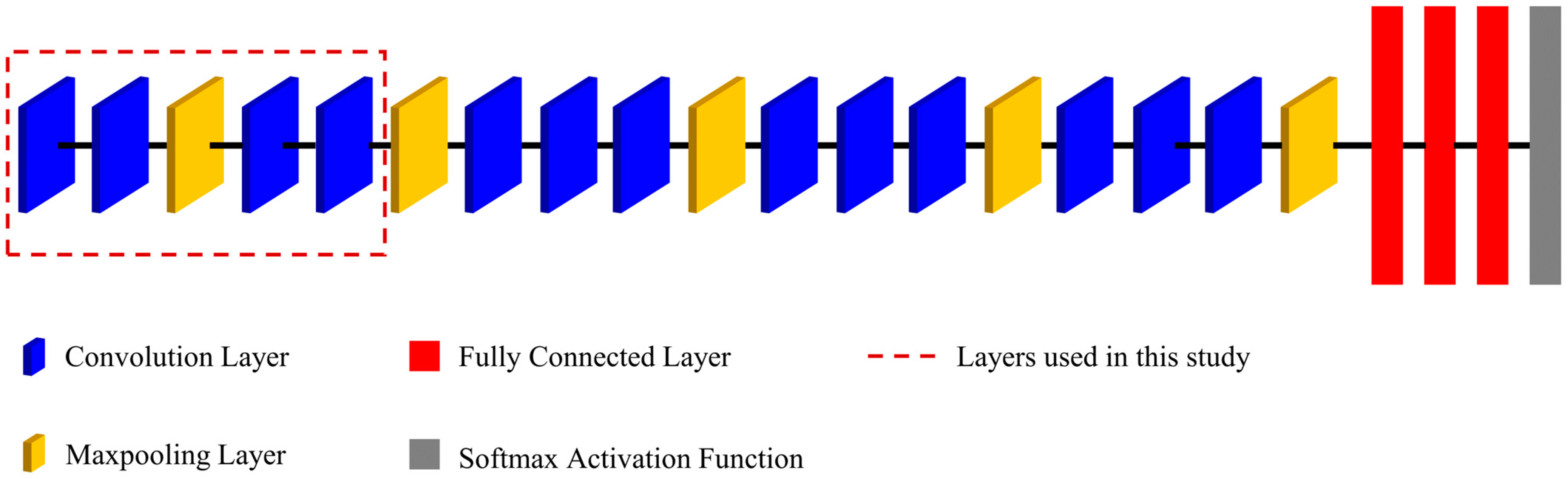
DCNNs, also referred to as atrous CNNs, involve the expansion of the convolutional kernel by introducing holes between its elements [19]. These holes, or dilations, enable the convolutional layer to access a larger area (field of view) of the input without increasing the number of parameters [41]. This mechanism allows for the capture of more contextual and multi-scale information. In DCNN, a crucial additional parameter, known as the dilation rate (DR), determines the spacing between the kernel’s sampled points. Equation (2) illustrates the operation of dilated convolution with input image $I$ and kernel $K$, where the parameters m and n represent the dimensions of $K$, and $r$ is the DR:

$$FeatureMap=I\times Kernel={\displaystyle \sum }_m{\displaystyle \sum }_{n}I\left(m,n\right)K\left(i\times r-m,j\times r-n\right)$$

(2)

2.4.2. VGG16

The VGG network, developed by the Visual Geometry Group at the University of Oxford, represents a CNN architecture [42]. In a competition where the group introduced six deep CNNs, VGG16 and VGG19 emerged as the most successful. VGG16 consists of 13 convolutional layers and three fully connected layers, while VGG19 includes 16 convolutional layers and three fully connected layers. Both networks employ a sequence of small 3 × 3 convolutional filters with a stride of 1, followed by multiple layers introducing non-linearity. For feature extraction in the encoder section of our proposed model, we used the initial five layers of VGG16, as depicted in Figure 4.

2.5. Attention Mechanism (AM)

In recent years, AMs have achieved significant attention in the field of DL, particularly for computer vision tasks such as object detection [28,30,43], image captioning [36,44,45], and action recognition [46,47]. The fundamental concept behind these mechanisms revolves around identifying the most crucial elements within input data while minimizing redundancy in the context of computer vision applications [30]. This process can be formalized as follows [48]:

$$Attention=f\left(g\left(x\right),x\right)$$

(3)

where $g\left(x\right)$ refers to generating attention, which involves focusing on the distinctive areas. The expression $f\left(g\left(x\right),x\right)$ denotes the action of handling input $x$ while considering the attention defined by $g\left(x\right)$. This process aligns with the idea of addressing crucial areas and extracting valuable information [48]. Almost all existing AMs can be written into the above formulation [48]. In this study, we employed CA, SA, and a ViT model that incorporates multi-head self-attention mechanism (MHSeA).

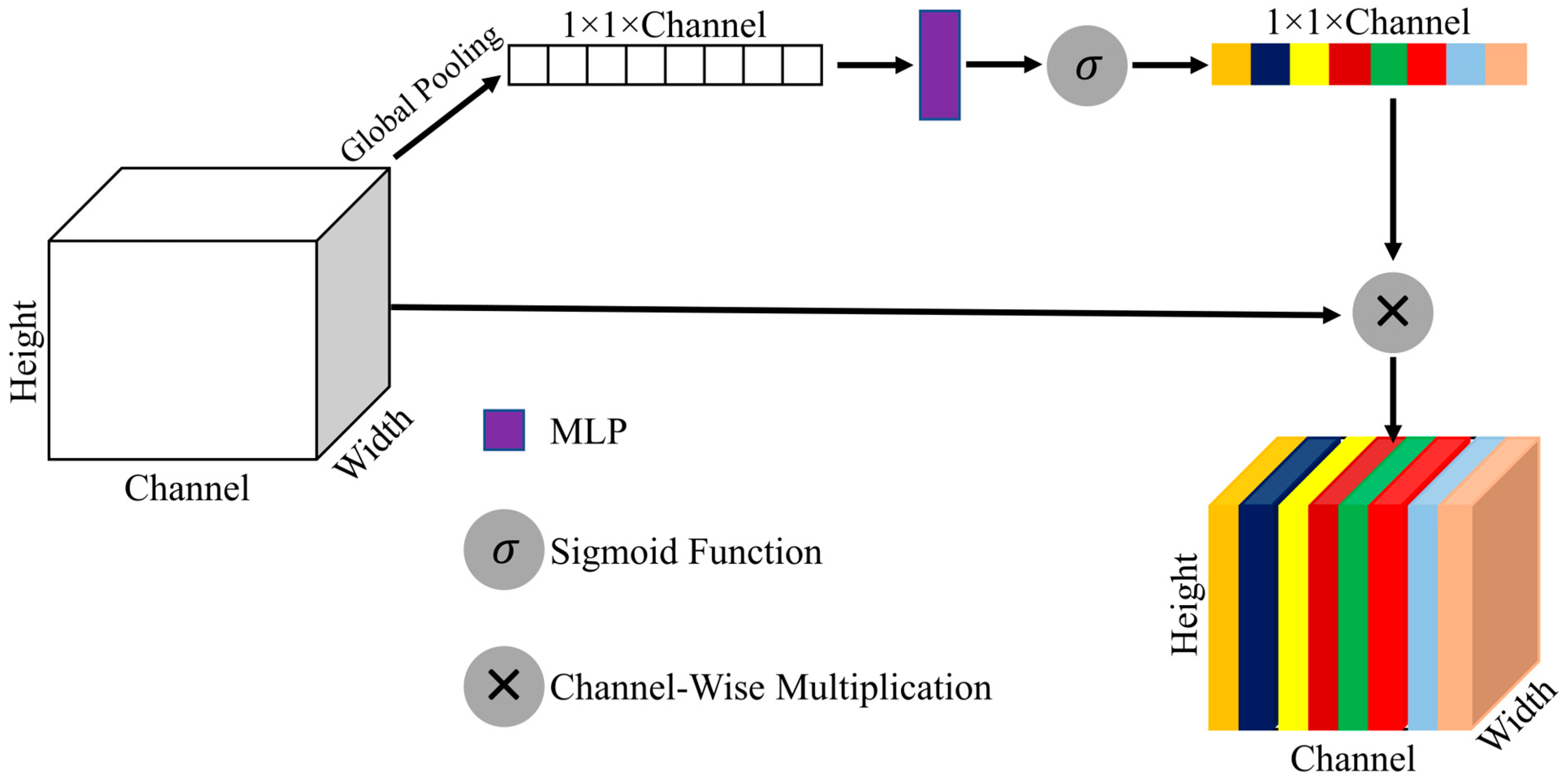
2.5.1. Channel Attention (CA)

In a typical CNN model, input data is processed by various convolution kernels, generating new channels with varying levels of information. CA introduces assigning weights to each channel to indicate the relevance between the channel and critical information. Higher weights signify greater relevance, directing the model’s attention to the corresponding channel [49]. CA enables the model to determine which channels to focus on autonomously.

As shown in Figure 5, the input feature map is subjected to a global pooling operation, which reduces the spatial dimensions of the feature map, transforming it into a vector output. This output vector is then processed through a sigmoid function, a key component that introduces non-linearity into the model. The resulting vector is channel-wise multiplied by the input feature map, producing a feature map where the importance of channels is explicitly defined.

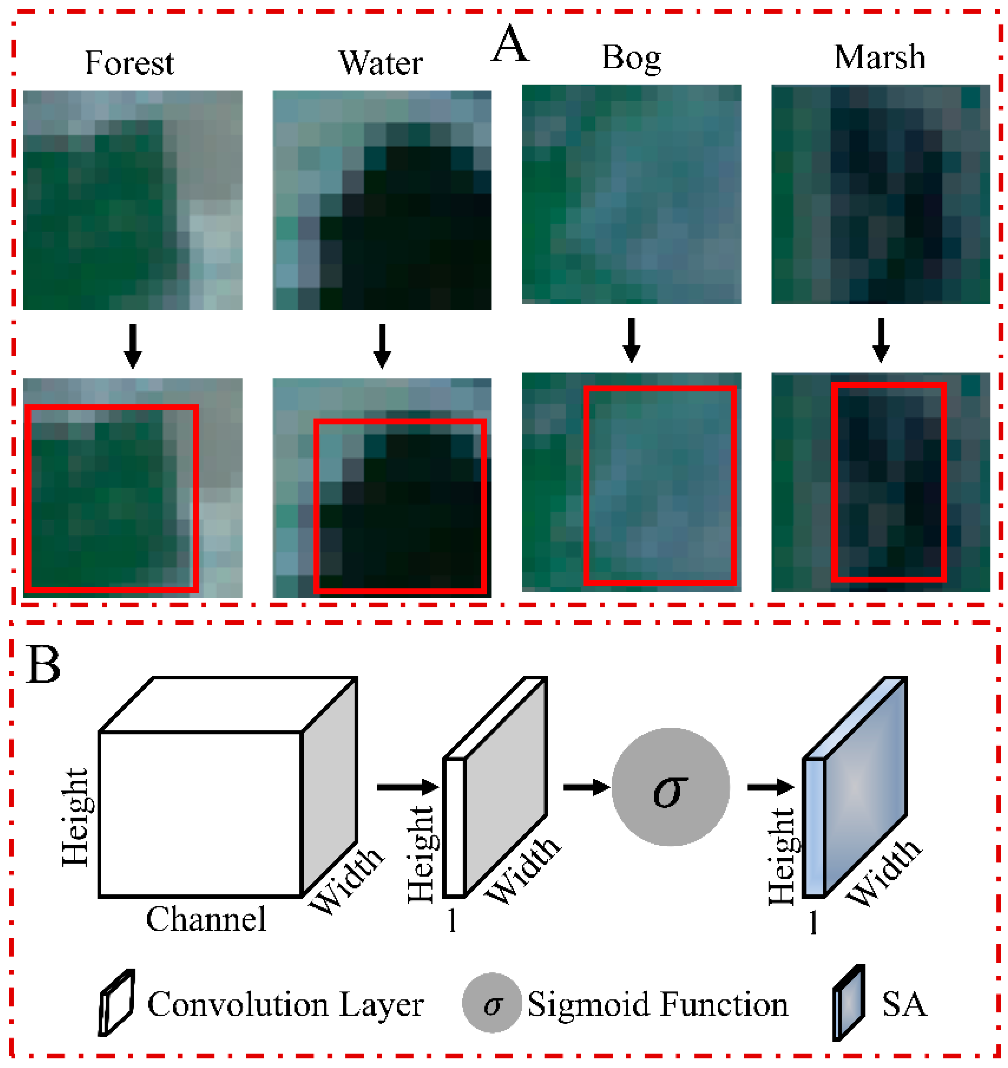
2.5.2. Spatial Attention (SA)

SA plays a pivotal role in enhancing the discernment capabilities of neural networks by enabling them to autonomously identify and prioritize relevant regions within the input data (refer to Figure 6A). This AM operates by transforming the spatial information inherent in the input data into a distinct space, thereby preserving essential information and significantly augmenting the network’s proficiency in object and pattern recognition [50].

In the SA mechanism, the input feature map transforms a 1 × 1 convolutional layer equipped with the sigmoid activation function and a singular filter. This convolutional operation is fundamental in discerning the significance of different spatial locations within the feature map. The resulting output from this process is then used to scale the input feature spatially, dynamically emphasizing regions deemed vital for the task at hand (refer to Figure 6B).

The intricate interplay of the 1 × 1 convolutional layer and sigmoid activation function allows the network to assign importance to spatial elements, promoting a refined understanding of the input’s spatial structure. This mechanism proves invaluable in capturing nuanced spatial relationships and is particularly effective in tasks where precise localization and discrimination of features are paramount.

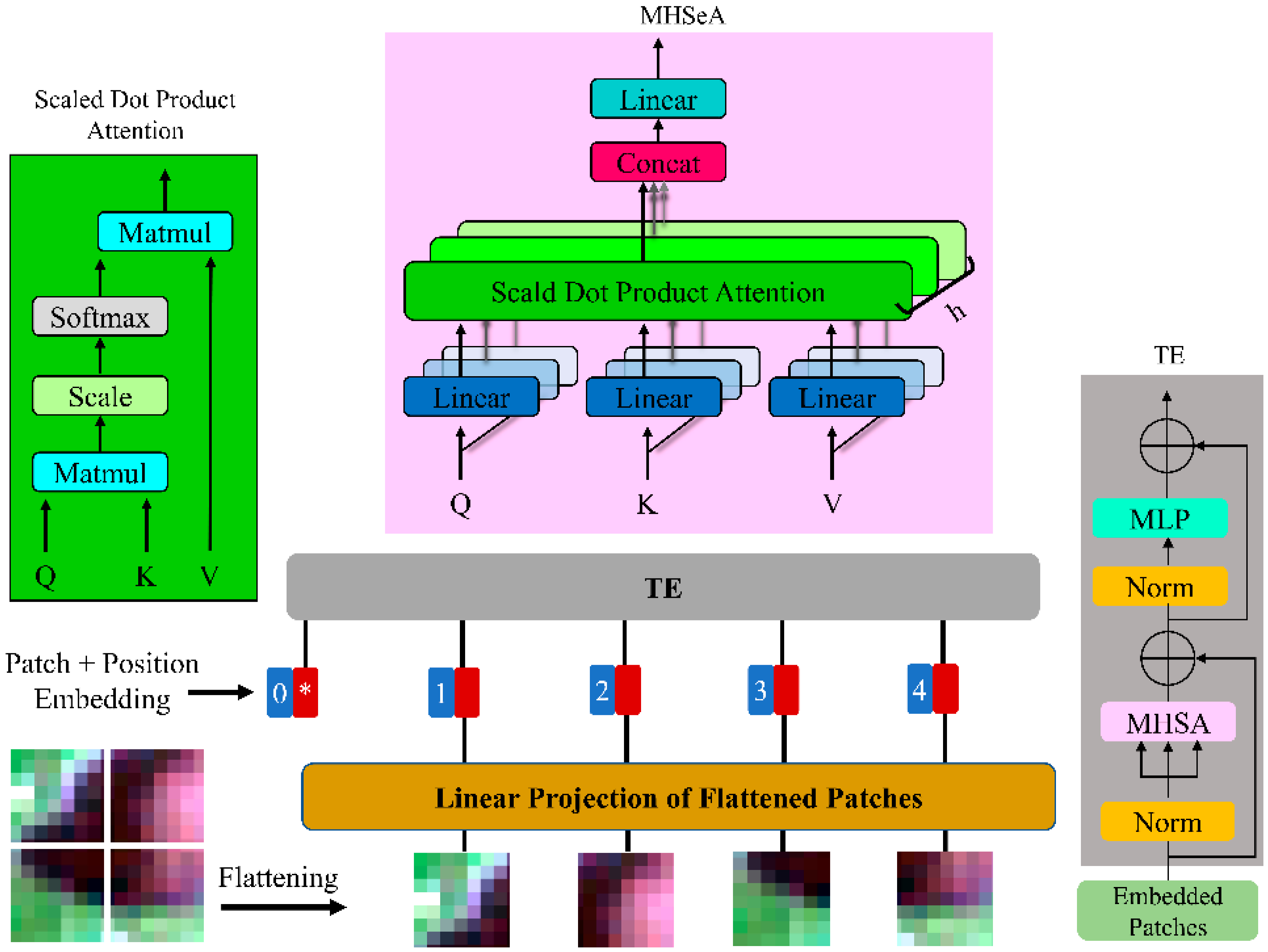
2.5.3. Self-Attention (SeA)

SeA is a core component of transformers that enables modeling relationships between all tokens in an input sequence. In ViT, SeA captures long-range dependencies between image patches and encodes interactions across the entire image. The key concept is to update a token’s representation by aggregating relevant global context from all other tokens [51]. For an input image $x$ of dimensions $H\times W\times C$ ($C$ is the number of channels, $H$ and $W$ are the height and width of the image, respectively), SeA first splits the image into $M$ flattened $2D$ patches $x_{p^{at}}$ of shape $M\times P^{2}C$, where $P$ is the patch size. These patches are projected into an embedding space of dimension $E$ using a learned linear layer, giving embeddings $X$ of shape $N\times E$. To apply SeA, $X$ is transformed into queries ($Q$), keys ($K$), and values ($V$) using separate projection matrices $W^Q$, $W^K$, and $W^V$. This allows modeling interactions between the $M$ patch embeddings. The sequence $X$ is projected to obtain $Q=X{W}^Q$, $K=X{W}^K$, and $V=X{W}^V$. Equation (4) indicates how the attention matrix $A$ of size $M\times M$ will be computed [52].

$$A=softmax\left(\frac{Q{K}^T}{\sqrt{E_q}}\right)V$$

(4)

2.5.4. Multi-Head Self-Attention (MHSeA)

MHSeA involves combining multiple SeA blocks that are concatenated in a channel-wise manner simultaneously [52]. This approach aims to capture diverse and complex relationships between various sequences of embeddings. Each head within the MHSeA possesses its unique set of learnable weight matrices, denoted as $W^{Q_i}$, $W^{K_i}$, and $W^{V_i}$, where $i$ ranges from $0$ to $h-1$, and $\mathrm{h}$ represents the number of heads in the MHSeA. This configuration enables the MHSeA to simultaneously attend to multiple aspects of the input data, using distinct sets of learned parameters for each head. Consequently, the model obtains the capacity to discern complex patterns and relationships, enhancing its ability to extract meaningful information distributed across various pixels.

2.5.5. Vision Transformer (ViT)

Recently, transformer-based models have shown remarkable performance in a wide range of applications, including computer vision and NLP. These transformers employ SeA mechanisms to effectively capture long-range dependencies [53]. In response to these advancements, [54] introduced ViT for image classification tasks. The ViT can capture extensive connections within input images [54]. It interprets images as a series of patches and utilizes a traditional transformer encoder. The ViT model comprises three main elements, namely: (1) patch embedding, (2) transformer encoder (TE), and (3) the classification head, as illustrated in Figure 7.

In the ViT architecture, the input image will be processed by first splitting it into a set number of non-overlapping image patches of equal dimensions. Then, these image patches will be flattened into 1D vectors that encode raw pixel values. Next, the linear projection will be applied to the patch vectors to derive lower-dimensional patch embedding representations. This projection step reduces the vector dimensionality while distilling the information contained in the original image patches into more compact feature vectors. The sequence of patch embeddings serves as the input to the TE.

The TE module is made up of several layers, each of which contains a MHSeA mechanism and a feedforward neural network. When encoding each patch, the SeA mechanism allows the model to pay attention to different parts of the image. The output of the SeA mechanism is transformed nonlinearly by the feedforward neural network. After passing through the TE, the sequence of embeddings is passed to an MLP, which predicts the class label of the input image.

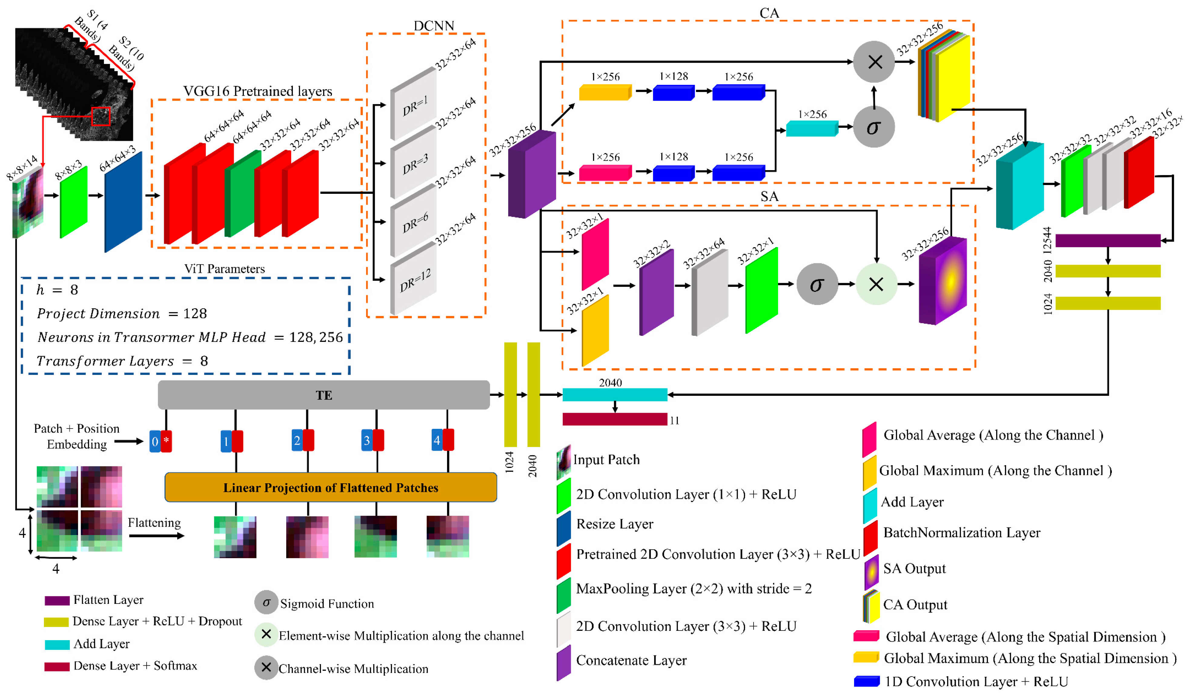
2.6. The Proposed Model (CVTNet)

In this study, we introduce a novel model named CVTNet, a convolutional ViT hybrid designed specifically for mapping wetlands using data from S1 and S2 satellites. The CVTNet model comprises two main branches: a convolutional branch and a ViT branch, as depicted in Figure 8.

The input image dimensions for the CVTNet model are set at 8 × 8 × 14. The initial stage employs a convolutional layer with three filters and a 1 × 1 kernel to align the number of channels with the three-channel input requirement of the VGG16 architecture. Subsequently, a resizing layer transforms the output dimensions to 64 × 64 × 3. The first five pre-trained layers of the VGG16 architecture encode the input image. This encoded output feeds into a DCNN module, featuring four convolutional layers with 64 filters and varying dilation rates (1, 3, 4, and 6). This module extracts multi-scale features from the encoded tensor, enhancing the field of view, and concatenates these features along the channels.

Given the varied weights and importance of multi-scale features, SA and CA are used to specify the importance of regions and channels, respectively. In both mechanisms, global average and global maximum operations are applied along channel and spatial dimensions, respectively. The CA mechanism employs 1D CNNs instead of traditional dense layers to extract more meaningful features for assessing feature importance. The features from the global average and maximum operations are combined through an added layer.

In the SA mechanism, global average and global maximum results are concatenated along their respective channels. This concatenated tensor undergoes a 2D convolutional layer with 64 filters. Subsequently, a convolutional layer with one filter and a 1 × 1 kernel, along with a sigmoid function, generates a heatmap. This heatmap scales the initial input feature map. The outputs from both CA and SA mechanisms are then integrated using an add layer.

Next, three convolutional layers with filter sizes of 32, 32, and 16 are employed to decode the extracted features. A batch normalization layer is used to normalize the features, ensuring that the mean output is close to 0 and the output standard deviation is close to 1, which enhances the stability of the optimization process. Finally, the extracted features are flattened using a flattened layer, and two dense layers with 2048 and 1024 neurons are used as the final layers in the first branch. It is worth noting that all convolution layers and dense layers in this branch are activated using the Rectified Linear Unit (ReLU) activation function.

The second branch of CVNet starts by dividing input images into nine non-overlapping patches, each with a size of 4 × 4 × 14. These patches are then flattened and encoded individually. The encoding process involves a positional embedding step. In this step, an embedding layer is employed to generate embeddings for each patch, mapping them to a lower-dimensional space (128).

CVNet’s second branch consists of eight layers of transformer blocks, each comprising several stages (see Figure 7 and Figure 8). First, a normalization layer is applied to the encoded patches. Then, MHSeA is used to capture relationships between the patches. The output of the MHSeA mechanism is combined with the encoded patches from the previous step, followed by another layer normalization (see Figure 7). An MLP processes the output of the MHSeA, which includes dense layers with ReLU activation functions and dropout with a rate of 0.1 (see Figure 7). Finally, the output of this process passes through dense layers with 2048 and 1024 neurons, utilizing ReLU activation functions and dropout with a 0.1 dropout rate (see Figure 8).

The second branch of CVTNet starts by dividing input images into nine non-overlapping patches, each with a size of 4 × 4 × 14. These patches are then flattened and encoded individually. The encoding process involves a positional embedding step. In this step, an embedding layer is employed to generate embeddings for each patch, mapping them to a lower-dimensional space (128).

CVTNet’s second branch consists of eight layers of transformer blocks, each comprising several stages (see Figure 7 and Figure 8). First, a normalization layer is applied to the encoded patches. Then, MHSeA is used to capture relationships between the patches. The output of the MHSeA mechanism is combined with the encoded patches from the previous step, followed by another layer normalization (see Figure 7). An MLP processes the output of the MHSeA, which includes dense layers with ReLU activation functions and dropout with a rate of 0.1. Finally, the output of this process passes through dense layers with 2048 and 1024 neurons (see Figure 8).

The outputs of the convolutional branch and the ViT branch are integrated using an add layer. Finally, there is a dense layer with 11 neurons and a softmax activation function used to classify the label of the input patch.

2.7. Validation Process

The validation of the CVTNet model employed a six-fold cross-validation (CV) strategy. The dataset D, comprising satellite image patches, was partitioned into six exclusive folds $D_1, D_2,\dots , D_6$. The model was trained six times, each time using the entire dataset except for one-fold reserved for validation. This resulted in 83% of the data (12,718 patches) being used for training and 17% (2604 patches) for validation in each iteration. The number of folds was determined through trial and error to balance robust validation and computational efficiency. Figure 9 illustrates the six-fold CV process.

To evaluate the performance of the CVTNet model, we used several metrics: F1-Score (F1), Kappa Coefficient (KC), Overall Accuracy (OA), Precision, and Recall. OA measures the proportion of correctly classified regions within the entire image, calculated by dividing the number of correctly classified pixels by the total number of pixels. The KC indicates the level of agreement between the reference data and the classified map, providing a normalized assessment of classification accuracy. The F1 score, crucial for imbalanced data, balances Precision and Recall. Precision (positive predictive value) reflects the accuracy of detected pixels for each class, avoiding false positives. Recall (sensitivity) shows how many actual pixels in each class are correctly classified, emphasizing the model’s ability to capture all relevant instances.

2.8. Occlusion Sensitivity

Occlusion sensitivity maps [55] were employed to identify key regions within the input image that significantly influence the classification decisions made by CVTNet. Occlusion sensitivity obscures sections of the input image using an occluding mask, such as a gray square and measures the change in the probability score for a particular class as the mask’s position varies. These maps highlight areas that substantially impact the classification score and those that contribute less or not at all. Figure 10 illustrates the procedure for generating heatmaps using the CVTNet model.

2.9. Experimental Settings

The CVTNet model was trained and tested using the Tensorflow [56] and Keras [57] packages on a machine with an Intel i7-10750H 2.6 GHz processor, 16 GB of RAM, and an NVIDIA GTX 1650 Ti graphics card. For the training phase, a batch size of 4 was determined through a trial-and-error approach. Furthermore, we used the Adam optimizer [58] with a learning rate of 0.0003 and binary cross-entropy for training the CVTNet model.

To prevent overfitting of the CVTNet model to the training data within the 200 iterations, we implemented the early stopping technique [59]. In each iteration using the training dataset, an evaluation was carried out on the validation dataset. If the model’s accuracy during validation was higher than any previously recorded maximum loss, the model’s weights were adjusted accordingly. Ultimately, at the conclusion of the training process, the most optimal model was saved.

3. Results

3.1. Quantitative Results

The performance of the proposed CVTNet model in mapping wetland areas using S1 and S2 satellite data was evaluated on both the training and validation datasets (see

Table 4. The CVTNet performance results based on both training and testing datasets.

Dataset	Metric
	OA	KC	F1	Recall	Precision
Validation	0.925	0.899	0.911	0.923	0.898
Training	0.961	0.936	0.942	0.961	0.924

). The model achieved a remarkable OA of 0.961 on the training set and 0.925 on the validation set. These high OA values highlight the model’s ability to accurately classify regions within the study area. Moreover, the model attained a KC of 0.936 on the training set and 0.899 on the validation set, demonstrating consistent and reliable performance in classifying wetland regions.

In dealing with the inherent challenges of imbalanced training data, CVTNet exhibits a balanced trade-off between Precision and Recall. The F1-Score, which harmonizes these two metrics, was 0.942 on the training dataset and 0.911 on the validation dataset. This balance is crucial for achieving accurate wetland mapping, where both the detection of actual wetland pixels (Recall) and the avoidance of false positives (Precision) are vital. Additionally, a detailed breakdown of Recall and Precision values provides knowledge about the model’s performance at the class level. The model’s high Recall (0.961) on the training set and substantial Recall (0.923) on the validation set underscore its high performance in correctly identifying true positive instances of wetland regions. Similarly, Precision values of 0.924 on the training set and 0.898 on the validation set indicate the model’s ability to minimize false positives.

The results in

Table 5. The performance of the CVTNet model for each individual class with F1, Precision, and Recall metrics.

Class	Training			Validation
	Recall	Precision	F1	Recall	Precision	F1
Bog	0.97	0.95	0.96	0.96	0.94	0.95
Exposed	0.87	0.83	0.85	0.78	0.78	0.78
Fen	0.99	0.95	0.97	0.93	0.93	0.93
Forest	0.94	0.98	0.96	0.94	0.94	0.94
Grassland	0.95	0.83	0.89	0.81	0.91	0.86
Marsh	0.92	0.94	0.93	0.89	0.89	0.89
Pasture	1	0.96	0.98	1	0.88	0.94
Shrubland	1	0.94	0.97	1	0.94	0.97
Swamp	0.95	0.97	0.96	0.91	0.97	0.94
Urban	1	1	1	0.98	1	0.99
Water	1	1	1	1	0.94	0.97

showcase the classification performance of the CVTNet model across different wetland classes, with a focus on key metrics including Recall, Precision, and F1-Score. In the training dataset, notable achievements are observed, particularly in classes like pasture, shrubland, urban, and water, where the model achieves perfect Recall (1.0), Precision (1.0), and F1-Score (1.0) values. The model also demonstrates strong performance in correctly identifying classes such as bog (Recall: 0.97, Precision: 0.95, F1: 0.96), fen (Recall: 0.99, Precision: 0.95, F1: 0.97), and forest (Recall: 0.94, Precision: 0.98, F1: 0.96). However, it exhibits some challenges in classes like exposed (Recall: 0.87, Precision: 0.83, F1: 0.85) and grassland (Recall: 0.95, Precision: 0.83, F1: 0.89), where Precision is comparatively lower.

For the validation dataset, the CVTNet continues to exhibit commendable performance, maintaining high Recall, Precision, and F1-Score values across several wetland classes. Classes like pasture, shrubland, urban, and water once again stand out with excellent performance metrics (Recall, Precision, and F1-Score all equal to 1.0). The model shows robustness in correctly classifying diverse wetland types, including bog (Recall: 0.96, Precision: 0.94, F1: 0.95), fen (Recall: 0.93, Precision: 0.93, F1: 0.93), forest (Recall: 0.94, Precision: 0.94, F1: 0.94), marsh (Recall: 0.89, Precision: 0.89, F1: 0.89), and swamp (Recall: 0.91, Precision: 0.97, F1: 0.94). Nevertheless, there are slight variations in Precision for certain classes, such as exposed (Recall: 0.78, Precision: 0.78, F1: 0.78) and grassland (Recall: 0.81, Precision: 0.91, F1: 0.86), indicating potential areas for improvement.

3.2. Models Results Comparison

To evaluate the efficacy of our proposed CVTNet model, we conducted a comparative analysis with contemporary algorithms in the realms of remote sensing and computer vision, including the ViT [54], MLP-mixer [60], hybrid spectral net (HybridSN) [61], and Random Forest (RF) [7] classifiers using the validation dataset.

Table 6. Results of the DL algorithms of the RF, ViT, MLP-mixer, HybridSN, and the proposed CVTNet in terms of OA, F1, and KC based on the validation patches and PB validation dataset.

Model	Metric
	OA	KC	F1	Recall	Precision
RF	0.815	0.751	0.779	0.743	0.819
ViT	0.862	0.839	0.847	0.857	0.838
MLP-mixer	0.884	0.856	0.872	0.882	0.864
HybridSN	0.762	0.725	0.749	0.761	0.739
CVTNet	0.921	0.899	0.911	0.923	0.898

presents key performance metrics, including OA, KC, F1, Recall, and Precision, for these models. Notably, the proposed CVTNet model outperformed state-of-the-art algorithms, achieving the highest OA of 0.921, along with a KC of 0.899, F1 of 0.911, Recall of 0.923, and Precision of 0.898. These detailed metrics highlight the superior performance of CVTNet in accurately classifying wetland areas compared to other evaluated models.

These comparative results demonstrated that the CVTNet model outperforms the other models in accuracy. This performance can be attributed to several key factors. CVTNet uses CNNs and the ViT algorithm. While CNNs are highly useful in extracting local spatial features, ViT excels at modeling long-range dependencies. The hybrid architecture allows CVTNet to use local and global features, leading to more accurate wetland mapping. The model’s ability to extract multi-scale features from S1 and S2 data improves its robustness. By combining data from S1 with S2, CVTNet benefits from complementary information, resulting in improved classification performance. Additionally, the AM in ViT enables CVTNet to focus on the most relevant parts of the input data, improving its ability to distinguish between wetlands and other land cover types. This targeted focus reduces misclassifications and improves overall mapping accuracy.

Furthermore, Figure 11 indicates the classification map obtained using these models. The visual analysis of these wetland maps shows that the CVTNet model successfully differentiated between non-wetlands and wetlands, demonstrating superior accuracy, particularly in classifying smaller objects.

4. Discussion

4.1. Attention Mechanism Effects and Sensitivity Analysis

Wetlands exhibit complicated land cover patterns with significant variability within classes and minimal differences between classes, presenting challenges for traditional ML algorithms used in classification tasks [7]. Overcoming these challenges requires innovative approaches. In this investigation, we introduced a novel DL model, CVTNet, comprising two key sections: CNN and ViT. The CNN section was employed to extract high-level features from S1 and S2 satellite data. To enhance feature extraction, we incorporated CA and SA mechanisms, directing CNN’s focus toward discerning features that distinguish wetland classes. To understand the impact of these mechanisms, we trained the CVTNet model both with and without CA and SA. Figure 12 provides a visualization of the Grad-CAM algorithm [62] output applied to concatenate layers in the CNN section for wetland and non-wetland classes under different attention conditions.

As depicted in Figure 12, the inclusion of CA and SA mechanisms in CVTNet proved crucial for discerning the unique characteristics of each class in an image patch. These heatmaps highlight the regions of image patches that significantly influenced CVTNet’s classification decisions. Under conditions where CA and SA mechanisms were absent, the model struggled to focus on relevant regions. In contrast, the presence of SA and CA mechanisms directed the model’s attention to key areas, highlighting their importance in improving model performance. This analysis underscores the effectiveness of AMs in guiding the model’s focus toward pertinent information within image patches.

The ViT model constitutes the second pivotal component of the CVTNet architecture. Its initial phase involves the division of image patches into a set of sub-patches with the aim of discerning the regions within the image contributing most significantly to the decisions made by the CVTNet model. To clarify the influence of these sub-patches on the model’s predictions, we employed the occlusion sensitivity method. Figure 13 provides samples of image patches for each wetland and non-wetland class, accompanied by the corresponding occlusion sensitivity output maps.

The showcased sample patches in Figure 13 indicate sensitivity in crucial regions across the entire patch, highlighting the ViT’s efficacy in concentrating on relevant areas. The occlusion sensitivity maps show that the ViT prioritizes the most influential regions within the patches. However, the CVTNet model assigns prominence to forests in certain classes like shrubland and grassland. Similarly, the CVTNet model is sensitive to the bog in the swamp class instead of swamps. These results confirm that there is an overlap between classes. However, unlike previous studies [2,4], this overlap is negligible between wetland classes. Moreover, the CVTNet model increases the synergy between features extracted from the CNN and ViT sections. This key feature can lead to optimizing the model’s ability to discern significant features across diverse wetland classes.

4.2. Investigating the Model’s Performance at the Class Boundaries

Unlike previous studies [3,11,63,64] that often emphasized overall accuracy without exploring the nuances at the wetland class peripheries, evaluating the performance of DL-based models in these edge cases is imperative. While specific studies boasted high accuracy in classifying wetland types, they should have addressed the inherent complexities at class boundaries, where seamless transitions between different wetland classes may occur. This section examines how the CVTNet model behaves with the pixels located at the edge of two classes.

Upon a more detailed examination of Figure 3, it becomes clear that, despite certain constraint conditions (e.g., $A$ > $A^{\prime }$), a few patches might remain without labels because they were at the edge of the wetland classes, and they were not used in the training phase. Therefore, we can assess the model’s performance using these boundary pixels. Figure 14 shows examples of these boundary pixels.

Upon scrutinizing the CVTNet model’s performance for these boundary pixels, significant challenges in accurately predicting classes become apparent. Figure 15 depicts the confusion matrix for these boundary pixels. Notably, the model encounters difficulties in distinguishing between bog and fen classes, as evidenced by 96 bog pixels out of 385 being misclassified as fen. Similarly, 104 out of 524 swamp pixels are erroneously classified as forest pixels. However, some classes, such as pasture, urban, grassland, and forest, exhibit correct classifications. These findings underscore that, while the CVTNet model achieved a high level of accuracy on the validation dataset, there remains room for improvement, particularly in handling boundary pixels. Addressing this challenge at the interface of two classes emerges as a pivotal focus for future studies in advancing wetland mapping accuracy.

5. Conclusions

In this study, we introduced and evaluated the CVTNet model for wetland mapping using S1 and S2 satellite data. The proposed model, integrating CNN and ViT algorithms, demonstrated exceptional performance in accurately classifying diverse wetland areas. The incorporation of AMs, including CA and SA, proved instrumental in enhancing the model’s ability to discern intricate features within image patches, leading to superior classification accuracy in the complex wetland environment.

The quantitative results showcased remarkable OA values of 0.961 on the training set and 0.925 on the validation set, highlighting the model’s efficacy in classifying wetland regions. Moreover, the model exhibited a balanced trade-off between Precision and Recall, crucial for accurate wetland mapping. The comparison with contemporary algorithms, including ViT, MLP-mixer, HybridSN, and Random Forest, reaffirmed the superior performance of CVTNet across various metrics.

Detailed analyses, such as sensitivity maps and examination of model performance at class boundaries, provided valuable insights. AMs were found to significantly impact the model’s focus, especially in discerning the unique characteristics of wetland classes. Challenges at class boundaries were identified, emphasizing the need for further improvement in handling transitional areas between different wetland classes. Future research could focus on refining the model’s performance at class boundaries and exploring additional AMs for further improvement in accuracy.

References

1. Jamali, A.; Mahdianpari, M.; Brisco, B.; Mao, D.; Salehi, B.; Mohammadimanesh, F. 3DUNetGSFormer: A deep learning pipeline for complex wetland mapping using generative adversarial networks and Swin transformer. Ecol. Inform. 2022, 72, 101904. [Google Scholar] [CrossRef]
2. Jamali, A.; Mahdianpari, M.; Mohammadimanesh, F.; Brisco, B.; Salehi, B. 3-D hybrid CNN combined with 3-D generative adversarial network for wetland classification with limited training data. IEEE J. Sel. Top. Appl. Earth Obs. Remote Sens. 2022, 15, 8095–8108. [Google Scholar] [CrossRef]
3. Jamali, A.; Mahdianpari, M. Swin transformer and deep convolutional neural networks for coastal wetland classification using sentinel-1, sentinel-2, and LiDAR data. Remote Sens. 2022, 14, 359. [Google Scholar] [CrossRef]
4. Mahdianpari, M.; Salehi, B.; Rezaee, M.; Mohammadimanesh, F.; Zhang, Y. Very deep convolutional neural networks for complex land cover mapping using multispectral remote sensing imagery. Remote Sens. 2018, 10, 1119. [Google Scholar] [CrossRef]
5. Rezaee, M.; Mahdianpari, M.; Zhang, Y.; Salehi, B. Deep convolutional neural network for complex wetland classification using optical remote sensing imagery. IEEE J. Sel. Top. Appl. Earth Obs. Remote Sens. 2018, 11, 3030–3039. [Google Scholar] [CrossRef]
6. Lang, M.W.; Bourgeau-Chavez, L.L.; Tiner, R.W.; Klemas, V.V. 5 Advances in Remotely. In Remote Sensing of Wetlands: Applications and Advances; CRC Press: Boca Raton, FL, USA, 2015; p. 79. [Google Scholar]
7. Mahdianpari, M.; Salehi, B.; Mohammadimanesh, F.; Motagh, M. Random forest wetland classification using ALOS-2 L-band, RADARSAT-2 C-band, and TerraSAR-X imagery. ISPRS J. Photogramm. Remote Sens. 2017, 130, 13–31. [Google Scholar] [CrossRef]
8. Torres, R.; Snoeij, P.; Geudtner, D.; Bibby, D.; Davidson, M.; Attema, E.; Potin, P.; Rommen, B.; Floury, N.; Brown, M.; et al. GMES Sentinel-1 mission. Remote Sens. Environ. 2012, 120, 9–24. [Google Scholar] [CrossRef]
9. Henderson, F.M.; Lewis, A.J. Radar detection of wetland ecosystems: A review. Int. J. Remote Sens. 2008, 29, 5809–5835. [Google Scholar] [CrossRef]
10. Drusch, M.; Del Bello, U.; Carlier, S.; Colin, O.; Fernandez, V.; Gascon, F.; Hoersch, B.; Isola, C.; Laberinti, P.; Martimort, P.; et al. Sentinel-2: ESA’s optical high-resolution mission for GMES operational services. Remote Sens. Environ. 2012, 120, 25–36. [Google Scholar] [CrossRef]
11. Slagter, B.; Tsendbazar, N.-E.; Vollrath, A.; Reiche, J. Mapping wetland characteristics using temporally dense Sentinel-1 and Sentinel-2 data: A case study in the St. Lucia wetlands, South Africa. Int. J. Appl. Earth Obs. Geoinf. 2020, 86, 102009. [Google Scholar] [CrossRef]
12. DeLancey, E.R.; Simms, J.F.; Mahdianpari, M.; Brisco, B.; Mahoney, C.; Kariyeva, J. Comparing deep learning and shallow learning for large-scale wetland classification in Alberta, Canada. Remote Sens. 2019, 12, 2. [Google Scholar] [CrossRef]
13. Igwe, V.; Salehi, B.; Mahdianpari, M. Rapid Large-Scale Wetland Inventory Update Using Multi-Source Remote Sensing. Remote Sens. 2023, 15, 4960. [Google Scholar] [CrossRef]
14. Jafarzadeh, H.; Mahdianpari, M.; Gill, E.W. Wet-GC: A Novel Multimodel Graph Convolutional Approach for Wetland Classification Using Sentinel-1 and 2 Imagery with Limited Training Samples. IEEE J. Sel. Top. Appl. Earth Obs. Remote Sens. 2022, 15, 5303–5316. [Google Scholar] [CrossRef]
15. Hosseiny, B.; Mahdianpari, M.; Brisco, B.; Mohammadimanesh, F.; Salehi, B. WetNet: A spatial–temporal ensemble deep learning model for wetland classification using Sentinel-1 and Sentinel-2. IEEE Trans. Geosci. Remote Sens. 2021, 60, 1–14. [Google Scholar] [CrossRef]
16. Jamali, A.; Mahdianpari, M.; Brisco, B.; Granger, J.; Mohammadimanesh, F.; Salehi, B. Deep Forest classifier for wetland mapping using the combination of Sentinel-1 and Sentinel-2 data. GIScience Remote Sens. 2021, 58, 1072–1089. [Google Scholar] [CrossRef]
17. Hemati, M.A.; Hasanlou, M.; Mahdianpari, M.; Mohammadimanesh, F. Wetland mapping of northern provinces of Iran using Sentinel-1 and Sentinel-2 in Google Earth Engine. In Proceedings of the 2021 IEEE International Geoscience and Remote Sensing Symposium IGARSS, Brussels, Belgium, 11–16 July 2021; IEEE: Piscataway, NJ, USA, 2021; pp. 96–99. [Google Scholar]
18. Jamali, A.; Mahdianpari, M.; Brisco, B.; Granger, J.; Mohammadimanesh, F.; Salehi, B. Wetland mapping using multi-spectral satellite imagery and deep convolutional neural networks: A case study in Newfoundland and Labrador, Canada. Can. J. Remote Sens. 2021, 47, 243–260. [Google Scholar] [CrossRef]
19. Marjani, M.; Mahdianpari, M.; Mohammadimanesh, F. CNN-BiLSTM: A Novel Deep Learning Model for Near-Real-Time Daily Wildfire Spread Prediction. Remote Sens. 2024, 16, 1467. [Google Scholar] [CrossRef]
20. Merchant, M.; Bourgeau-Chavez, L.; Mahdianpari, M.; Brisco, B.; Obadia, M.; DeVries, B.; Berg, A. Arctic ice-wedge landscape mapping by CNN using a fusion of Radarsat constellation Mission and ArcticDEM. Remote Sens. Environ. 2024, 304, 114052. [Google Scholar] [CrossRef]
21. Taghizadeh-Mehrjardi, R.; Mahdianpari, M.; Mohammadimanesh, F.; Behrens, T.; Toomanian, N.; Scholten, T.; Schmidt, K. Multi-task convolutional neural networks outperformed random forest for mapping soil particle size fractions in central Iran. Geoderma 2020, 376, 114552. [Google Scholar] [CrossRef]
22. Mahdianpari, M.; Brisco, B.; Granger, J.; Mohammadimanesh, F.; Salehi, B.; Homayouni, S.; Bourgeau-Chavez, L. The third generation of pan-Canadian wetland map at 10 m resolution using multisource earth observation data on cloud computing platform. IEEE J. Sel. Top. Appl. Earth Obs. Remote Sens. 2021, 14, 8789–8803. [Google Scholar] [CrossRef]
23. Mohammadimanesh, F.; Salehi, B.; Mahdianpari, M.; Gill, E.; Molinier, M. A new fully convolutional neural network for semantic segmentation of polarimetric SAR imagery in complex land cover ecosystem. ISPRS J. Photogramm. Remote Sens. 2019, 151, 223–236. [Google Scholar] [CrossRef]
24. Alhichri, H.; Alswayed, A.S.; Bazi, Y.; Ammour, N.; Alajlan, N.A. Classification of remote sensing images using EfficientNet-B3 CNN model with attention. IEEE Access 2021, 9, 14078–14094. [Google Scholar] [CrossRef]
25. Kattenborn, T.; Leitloff, J.; Schiefer, F.; Hinz, S. Review on Convolutional Neural Networks (CNN) in vegetation remote sensing. ISPRS J. Photogramm. Remote Sens. 2021, 173, 24–49. [Google Scholar] [CrossRef]
26. Khan, M.A.; Akram, T.; Zhang, Y.-D.; Sharif, M. Attributes based skin lesion detection and recognition: A mask RCNN and transfer learning-based deep learning framework. Pattern Recognit. Lett. 2021, 143, 58–66. [Google Scholar] [CrossRef]
27. Cao, J.; Cui, H.; Zhang, Q.; Zhang, Z. Ancient mural classification method based on improved AlexNet network. Stud. Conserv. 2020, 65, 411–423. [Google Scholar] [CrossRef]
28. Simonyan, K.; Zisserman, A. Very deep convolutional networks for large-scale image recognition. arXiv 2014, arXiv:1409.1556. [Google Scholar]
29. He, K.; Zhang, X.; Ren, S.; Sun, J. Deep residual learning for image recognition. In Proceedings of the IEEE Conference on Computer Vision and Pattern Recognition, Las Vegas, NV, USA, 27–30 June 2016; pp. 770–778. [Google Scholar]
30. Vaswani, A.; Shazeer, N.; Parmar, N.; Uszkoreit, J.; Jones, L.; Gomez, A.N.; Kaiser, Ł.; Polosukhin, I. Attention is all you need. Adv. Neural Inf. Process. Syst. 2017, 30, 2440–2448. [Google Scholar]
31. Han, K.; Wang, Y.; Chen, H.; Chen, X.; Guo, J.; Liu, Z.; Tang, Y.; Xiao, A.; Xu, C.; Xu, Y.; et al. A survey on vision transformer. IEEE Trans. Pattern Anal. Mach. Intell. 2022, 45, 87–110. [Google Scholar] [CrossRef]
32. Bazi, Y.; Bashmal, L.; Rahhal, M.M.A.; Dayil, R.A.; Ajlan, N.A. Vision transformers for remote sensing image classification. Remote Sens. 2021, 13, 516. [Google Scholar] [CrossRef]
33. He, J.; Zhao, L.; Yang, H.; Zhang, M.; Li, W. HSI-BERT: Hyperspectral image classification using the bidirectional encoder representation from transformers. IEEE Trans. Geosci. Remote Sens. 2019, 58, 165–178. [Google Scholar] [CrossRef]
34. Hong, D.; Han, Z.; Yao, J.; Gao, L.; Zhang, B.; Plaza, A.; Chanussot, J. SpectralFormer: Rethinking hyperspectral image classification with transformers. IEEE Trans. Geosci. Remote Sens. 2021, 60, 1–15. [Google Scholar] [CrossRef]
35. Wu, F.; Fan, A.; Baevski, A.; Dauphin, Y.N.; Auli, M. Pay less attention with lightweight and dynamic convolutions. arXiv 2019, arXiv:1901.10430. [Google Scholar]
36. Wu, Z.; Liu, Z.; Lin, J.; Lin, Y.; Han, S. Lite transformer with long-short range attention. arXiv 2020, arXiv:2004.11886. [Google Scholar]
37. Gulati, A.; Qin, J.; Chiu, C.C.; Parmar, N.; Zhang, Y.; Yu, J.; Han, W.; Wang, S.; Zhang, Z.; Wu, Y.; et al. Conformer: Convolution-augmented transformer for speech recognition. arXiv 2020, arXiv:2005.08100. [Google Scholar]
38. Marjani, M.; Ahmadi, S.A.; Mahdianpari, M. FirePred: A hybrid multi-temporal convolutional neural network model for wildfire spread prediction. Ecol. Inform. 2023, 78, 102282. [Google Scholar] [CrossRef]
39. Marjani, M.; Mesgari, M.S. The large-scale wildfire spread prediction using a multi-kernel convolutional neural network. ISPRS Ann. Photogramm. Remote Sens. Spat. Inf. Sci. 2023, X-4/W1-2022, 483–488. [Google Scholar] [CrossRef]
40. Radman, A.; Mahdianpari, M.; Varon, D.J.; Mohammadimanesh, F. S2MetNet: A novel dataset and deep learning benchmark for methane point source quantification using Sentinel-2 satellite imagery. Remote Sens. Environ. 2023, 295, 113708. [Google Scholar] [CrossRef]
41. Liu, R.; Tao, F.; Liu, X.; Na, J.; Leng, H.; Wu, J.; Zhou, T. RAANet: A Residual ASPP with Attention Framework for Semantic Segmentation of High-Resolution Remote Sensing Images. Remote Sens. 2022, 14, 3109. [Google Scholar] [CrossRef]
42. Paymode, A.S.; Malode, V.B. Transfer learning for multi-crop leaf disease image classification using convolutional neural networks VGG. Artif. Intell. Agric. 2022, 6, 23–33. [Google Scholar] [CrossRef]
43. Ba, J.; Mnih, V.; Kavukcuoglu, K. Multiple Object Recognition with Visual Attention. arXiv 2014, arXiv:1412.7755. [Google Scholar]
44. Anderson, P.; He, X.; Buehler, C.; Teney, D.; Johnson, M.; Gould, S.; Zhang, L. Bottom-Up and Top-Down Attention for Image Captioning and Visual Question Answering. In Proceedings of the 2018 IEEE/CVF Conference on Computer Vision and Pattern Recognition, Salt Lake City, UT, USA, 18–23 June 2018; pp. 6077–6086. [Google Scholar]
45. Wu, H.; Xiao, B.; Codella, N.; Liu, M.; Dai, X.; Yuan, L.; Zhang, L. CvT: Introducing Convolutions to Vision Transformers. In Proceedings of the 2021 IEEE/CVF International Conference on Computer Vision (ICCV), Montreal, BC, Canada, 11–17 October 2021; pp. 22–31. [Google Scholar]
46. Sharma, S.; Kiros, R.; Salakhutdinov, R. Action Recognition using Visual Attention. arXiv 2015, arXiv:1511.04119. [Google Scholar]
47. Du, W.; Wang, Y.; Qiao, Y. Recurrent Spatial-Temporal Attention Network for Action Recognition in Videos. IEEE Trans. Image Process. 2018, 27, 1347–1360. [Google Scholar] [CrossRef] [PubMed]
48. Guo, M.-H.; Xu, T.-X.; Liu, J.-J.; Liu, Z.-N.; Jiang, P.-T.; Mu, T.-J.; Zhang, S.-H.; Martin, R.R.; Cheng, M.-M.; Hu, S.-M. Attention mechanisms in computer vision: A survey. Comput. Vis. Media 2021, 8, 331–368. [Google Scholar] [CrossRef]
49. Hu, J.; Shen, L.; Albanie, S.; Sun, G.; Wu, E. Squeeze-and-Excitation Networks. In Proceedings of the 2018 IEEE/CVF Conference on Computer Vision and Pattern Recognition, Salt Lake City, UT, USA, 18–23 June 2018; pp. 7132–7141. [Google Scholar]
50. Niu, Z.; Zhong, G.; Yu, H. A review on the attention mechanism of deep learning. Neurocomputing 2021, 452, 48–62. [Google Scholar] [CrossRef]
51. Marjani, M.; Mahdianpari, M.; Ahmadi, S.A.; Hemmati, E.; Mohammadimanesh, F.; Mesgari, M.S. Application of Explainable Artificial Intelligence in Predicting Wildfire Spread: An ASPP-Enabled CNN Approach. IEEE Geosci. Remote Sens. Lett. 2024. [Google Scholar] [CrossRef]
52. Aleissaee, A.A.; Kumar, A.; Anwer, R.M.; Khan, S.; Cholakkal, H.; Xia, G.-S.; Khan, F.S. Transformers in remote sensing: A survey. Remote Sens. 2023, 15, 1860. [Google Scholar] [CrossRef]
53. Khan, S.; Naseer, M.; Hayat, M.; Zamir, S.W.; Khan, F.S.; Shah, M. Transformers in Vision: A Survey. ACM Comput. Surv. 2021, 54, 1–41. [Google Scholar] [CrossRef]
54. Dosovitskiy, A.; Beyer, L.; Kolesnikov, A.; Weissenborn, D.; Zhai, X.; Unterthiner, T.; Dehghani, M.; Minderer, M.; Heigold, G.; Gelly, S.; et al. An Image is Worth 16 × 16 Words: Transformers for Image Recognition at Scale. arXiv 2020, arXiv:2010.11929. [Google Scholar]
55. Bolmer, E.; Abulaitijiang, A.; Kusche, J.; Roscher, R. Occlusion Sensitivity Analysis of Neural Network Architectures for Eddy Detection. In Proceedings of the IGARSS 2022—2022 IEEE International Geoscience and Remote Sensing Symposium, Kuala Lumpur, Malaysia, 17–22 July 2022; pp. 623–626. [Google Scholar]
56. Géron, A. Hands-On Machine Learning with Scikit-Learn and TensorFlow: Concepts, Tools, and Techniques to Build Intelligent Systems; O’Reilly Media, Inc.: Sebastopol, CA, USA, 2017. [Google Scholar]
57. Manaswi, N. Understanding and Working with Keras. In Deep Learning with Applications Using Python; Apress: Berkeley, CA, USA, 2018. [Google Scholar] [CrossRef]
58. Kingma, D.P.; Ba, J. Adam: A Method for Stochastic Optimization. arXiv 2014, arXiv:1412.6980. [Google Scholar]
59. Mahsereci, M.; Balles, L.; Lassner, C.; Hennig, P. Early Stopping without a Validation Set. arXiv 2017, arXiv:1703.09580. [Google Scholar]
60. Tolstikhin, I.O.; Houlsby, N.; Kolesnikov, A.; Beyer, L.; Zhai, X.; Unterthiner, T.; Yung, J.; Steiner, A.; Keysers, D.; Uszkoreit, J.; et al. MLP-Mixer: An all-MLP Architecture for Vision. Adv. Neural Inf. Process. Syst. 2021, 34, 24261–24272. [Google Scholar]
61. Roy, S.K.; Krishna, G.; Dubey, S.R.; Chaudhuri, B.B. HybridSN: Exploring 3-D–2-D CNN Feature Hierarchy for Hyperspectral Image Classification. IEEE Geosci. Remote Sens. Lett. 2019, 17, 277–281. [Google Scholar] [CrossRef]
62. Selvaraju, R.R.; Cogswell, M.; Das, A.; Vedantam, R.; Parikh, D.; Batra, D. Grad-CAM: Visual Explanations from Deep Networks via Gradient-Based Localization. Int. J. Comput. Vis. 2016, 128, 336–359. [Google Scholar] [CrossRef]
63. Jamali, A.; Mahdianpari, M.; Mohammadimanesh, F.; Homayouni, S. A deep learning framework based on generative adversarial networks and vision transformer for complex wetland classification using limited training samples. Int. J. Appl. Earth Obs. Geoinf. 2022, 115, 103095. [Google Scholar] [CrossRef]
64. Mahdianpari, M.; Rezaee, M.; Zhang, Y.; Salehi, B. Wetland classification using deep convolutional neural network. In Proceedings of the IGARSS 2018—2018 IEEE International Geoscience and Remote Sensing Symposium, Valencia, Spain, 22–27 July 2018; IEEE: Piscataway, NJ, USA; pp. 9249–9252. [Google Scholar]
Figure 1. A composite image, utilizing true color composites from Bing satellite imagery, showcases the geographical extent of the study area.
Remotesensing 16 02427 g001
Figure 2. The spatial distribution of the training and validation sets within the study area.
Remotesensing 16 02427 g002
Figure 3. The patch labeling process involved the utilization of two open-source tools: Python and GEE. The data collection process was executed using GEE, followed by the application of Python programming to assign labels to the central pixels of the patches.
Remotesensing 16 02427 g003
Figure 4. The architecture of the VGG16.
Remotesensing 16 02427 g004
Figure 5. Illustration of the CA mechanism. Different colors of the channels show their different importance.
Remotesensing 16 02427 g005
Figure 6. (A) There are four patch samples, and the SA mechanism focuses on the highlighted red area within each patch; and (B) a diagram demonstrating the functioning of the SA mechanism.
Remotesensing 16 02427 g006
Figure 7. The architecture of the ViT is depicted on the left, while the specifications of the encoder block are illustrated on the right and above. Initially, the input image is divided into patches. Subsequently, these patches are projected into a feature space after being flattened. Within this feature space, a TE analyzes them to generate the classification output. The presence of * denotes the incorporation of an additional learnable class embedding.
Remotesensing 16 02427 g007
Figure 8. The overall architecture of the CVNet model for wetland mapping. The presence of * denotes the incorporation of an additional learnable class embedding.
Remotesensing 16 02427 g008
Figure 9. The explanation of the implementation of a six-fold CV procedure for the dataset.
Remotesensing 16 02427 g009
Figure 10. The process of producing a heatmap through the occlusion sensitivity technique using 4 × 4 gray square masks. The M values represent the maximum values among the red vectors.
Remotesensing 16 02427 g010
Figure 11. (a) The S2 true color (RGB) of a region in the study area, (b) classified map using CVTNet, (c) MLP-mixer, (d) RF, (e) HubridSN, and (f) ViT.
Remotesensing 16 02427 g011
Figure 12. The Grad-CAM algorithm output with and without CA and SA mechanisms. The RGB images were derived from S2 satellite data.
Remotesensing 16 02427 g012
Figure 13. Sensitivity map for each individual wetland and non-wetland class. The multiplication symbol indicates pixels that contain the main class within the given patch.
Remotesensing 16 02427 g013
Figure 14. Examples of boundary pixels for each class.
Remotesensing 16 02427 g014
Figure 15. Confusion matrix for boundary pixels.
Remotesensing 16 02427 g015