Abstract
Monitoring inundation in flow-dependent floodplain wetlands is important for understanding the outcomes of environmental water deliveries that aim to inundate different floodplain wetland vegetation types. The most effective way to monitor inundation across large landscapes is with remote sensing. Spectral water indices are often used to detect water in the landscape, but there are challenges in using them to map inundation within the complex vegetated floodplain wetlands. The current method used for monitoring inundation in the large floodplain wetlands that are targets for environmental water delivery in the New South Wales portion of the Murray–Darling Basin (MDB) in eastern Australia considers the complex mixing of water with vegetation and soil, but it is a time-consuming process focused on individual wetlands. In this study, we developed the automated inundation monitoring (AIM) method to enable an efficient process to map inundation in floodplain wetlands with a focus on the lower Lachlan floodplain utilising 25 Sentinel-2 image dates spanning from 2019 to 2023. A local adaptive thresholding (ATH) approach of a suite of spectral indices combined with best available DEM and a cropping layer were integrated into the AIM method. The resulting AIM maps were validated against high-resolution drone images, and vertical and oblique aerial images. Although instances of omission and commission errors were identified in dense vegetation and narrow creek lines, the AIM method showcased high mapping accuracy with overall accuracy of 0.8 measured. The AIM method could be adapted to other MDB wetlands that would further support the inundation monitoring across the basin.
1. Introduction
Wetlands are ecologically significant parts of the landscape, characterised by periods of wetting (through overland flows or ground water) that are used by water-dependent flora and fauna in all or part of their lifecycle [1,2]. Floodplain wetlands are distinct wetlands that are highly dynamic and characterised by highly variable landscapes with complex channel networks, topographic depressions and vegetation mosaics. The configurations of these floodplain wetlands are largely influenced by extent of inundation, timing of flood pulses and flood frequency regimes [3]. Globally, floodplain wetlands are recognised for their significance in providing crucial habitat for freshwater aquatic ecological communities, influencing species richness, abundance and recruitment [3,4,5,6]. Ecosystem health and habitat availability are reliant on the inundation regimes from highly variable river flows [7]. However, inundation regimes in floodplain wetlands have been considerably altered due to climate change and human disturbance [8,9]. These disturbances include extraction of water from river systems, constraints within river systems that divert flows away from wetlands and land-use changes within and around the wetlands. In response, environmental flows have been implemented globally to support river flows and lateral connectivity to help restore the condition of floodplain wetlands [10].
Environmental flows have become an important tool in the management of rivers and floodplain wetlands in the Murray–Darling Basin [MDB] [11], which has experienced substantial declines in both wetland extent and condition. The establishment of the Basin Plan in 2012 was designed to manage water in a sustainable way, with the basin-wide environmental water strategy (BWS) developed to assist the implementation the objectives set out in the plan. This includes setting measurable outcomes that enable objective evaluation of the management of water and improve river flows and connectivity, to ultimately help improve and sustain water-dependent vegetation, fauna and fish communities [12,13]. Therefore, being able to monitor inundation across floodplain wetlands is crucial for environmental water management and assessing ecological outcomes across the basin [14,15,16,17].
Monitoring inundation is typically undertaken using satellite data that can be obtained from various sensor types. Inundation mapping has been undertaken using thermal [18], synthetic aperture radar [19] and optical data [20]. Synthetic aperture radar (SAR) data have become increasingly popular as they can be used under cloud cover and certain bands are able to penetrate vegetation [21], which is a significant limitation of optical sensors. However, optical sensors typically produce data at higher spatial resolutions than thermal sensors, while SAR data suffer from ‘speckling’ and geometric distortion [21]. Optical data are also captured with a greater spectral resolution than both SAR and thermal data, with Sentinel-2 sensors capturing data in visible, near-infrared and shortwave infrared wavelengths [22]. This broad spectral resolution provides flexibility to combine data obtained at different wavelengths into indices that enhance desired land cover characteristics.
To date, remote sensing indices have proven valuable in detecting and mapping surface water, particularly in open water bodies. This is evident in such indices as the Fisher water index (FWI) [23], the normalised difference water index (NDWIXu) [24] and the normalised difference water index (NDWIMcFeeters) [25]. When classifying pure, open water with optimised thresholds, these indices have shown overall accuracies >94%, making them suitable for use in automated processes to detect water bodies across large regions [23,24]. However, the accuracy of these indices when discriminating mixed pixels, which contain a mixture of water and other cover types, is reduced [23]. The ability to correctly detect the inundation status of vegetated areas is diminished even further [26]. Addressing these limitations within flooded forest communities has been achieved by selecting optimal indices and thresholds for specific land-cover types in the multi-index method (MIM) [27]. Other approaches have used adaptive thresholding techniques to classify water and inundated vegetation [28], while simple thresholds applied to near-infrared and shortwave infrared data have also proven effective [26]. Machine learning techniques have also been used, combining water and vegetation indices to predict inundation extent [29,30]. However, validation of these approaches has involved comparisons to existing Landsat-derived inundation maps [28,29] and the use of interpolated depth information [26], which may present uncertainties in assessing accuracy. Creating validation data using high-resolution satellite and airborne imagery, as Ticehurst et al. [27] did, may overcome these uncertainties, but their focus was on forest wetlands rather than densely vegetated non-woody wetlands. As such, it remains unclear what approach is best to classify the inundation status of wetland vegetation, highlighting an ongoing need for further research in this area.
One of several of products developed for monitoring inundation within Australia is the Digital Earth Australia Water Observations (DEA WO, formerly Water Observations from Space), developed by Geoscience Australia [31]. The results of Mueller et al. [31] demonstrated that DEA-WO performs well in capturing open water areas but did not adequately map inundation extent in vegetated wetlands. Dunn et al. [32] combined the DEA-WO product with tasseled cap wetness transform (TCW) and the fractional cover product [33] to create the Wetlands Insight Tool (WIT), which visualises changes in water and vegetation within individual wetlands. This tool leverages existing products to provide valuable, site-specific insights on both vegetation and inundation dynamics, but does not quantify the extent of inundated vegetation. The multi-index method (MIM) of Ticehurst et al. [27] was used in an ensemble with the DEA-WO to take the maximum extent of the combined products to improve performance [34]. However, limitations in detecting inundation within dense vegetation likely remain in the MIM product [27], meaning these limitations will extend into the ensemble. Such challenges have evolved due to the complex spectral response of wetland vegetation resulting in a high degree of mixed pixels (i.e., water with submerged vegetation) present as well as totally obscuring the spectral response of water, making inundation mapping using remotely sensed data difficult [35]. These studies demonstrate the complexity of detecting water under dense vegetation communities of the MDB wetlands.
A bespoke approach to mapping inundation in a vegetated floodplain wetland within the MDB, specifically the Macquarie Marshes, was demonstrated by Thomas et al. [36] using both water and vegetation indices to classify inundation classes. Thomas et al. [36] showed that for effective mapping of inundation, the threshold for detecting water from the modified NDWIXu [24] needed to be varied to incorporate mixed pixels. For dense emergent macrophyte vegetation that obscures water detection, vegetation indices were used to detect the phenological phases as a surrogate to inundation. The effectiveness of this method is evident in the inundation maps being used to monitor inundation extent in large floodplain wetlands as part of the Environmental Water Management Program [12]. The focus on an individual floodplain wetland (rather than an entire satellite scene) and the reliance on expert knowledge of vegetation community distribution contributes to its effectiveness. However, the need to vary spectral index thresholds is time-consuming, especially now with the increased frequency of return period offered by Sentinel-2. A more automated method is required to detect inundation while accommodating the complexity of vegetated floodplain wetlands located across the NSW portion of the MDB.
The objective of this study is to integrate multiple Sentinel-2-derived indices with LiDAR-derived digital elevation models (DEMs) into an automated model: the automated inundation monitoring (AIM) method, for effective mapping of inundation in wetlands. This study demonstrates that the AIM method can detect inundation in open water bodies, within mixed vegetation and under dense vegetation of floodplain wetlands. The outcome from this study is also expected to be further developed to map inundation across all available Sentinel-2 tiles of other floodplain wetlands of the NSW portion of the MDB improving both the spatial and temporal coverage of inundation mapping. The resulting inundation maps will help support decisions for environmental water delivery and allow other end-users to access an accurate inundation product across a diverse range of wetland landscapes.
2. Materials and Methods
2.1. Automated Inundation Monitoring
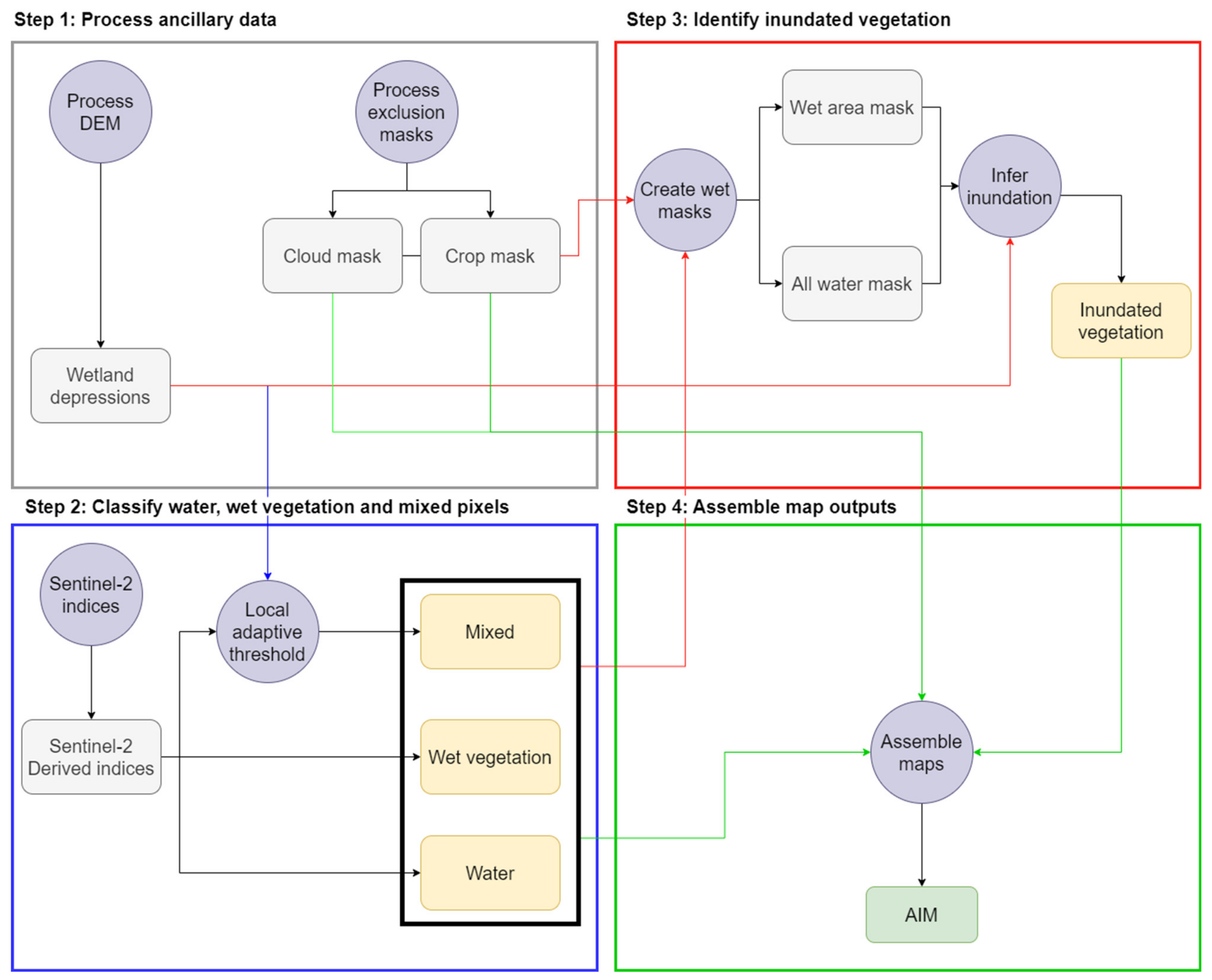
The automated inundation monitoring (AIM) approach consists of four discrete processes (Figure 1). The first process is performed once and involves the initialisation of ancillary data to constrain the classification process (step 1). This is followed by automated methods that classify inundated, mixed and wet vegetation, where wet vegetation is considered wetland vegetation that is either inundated or growing in moist soils (step 2). Masking of non-wetland areas, such as cropping areas and cloud shadows, is performed before using elevation to infer the inundation status of wetland vegetation (step 3). The final step involves combining all AIM classified outputs to produce the inundation map (step 4).
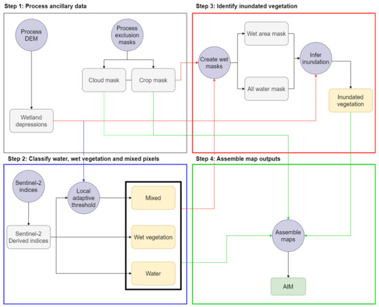
Figure 1.
Diagram demonstrating the automated inundation monitoring (AIM) method workflow. Coloured arrows indicate the step an output is flowing to. Grey boxes represent mask outputs, yellow boxes represent AIM class outputs and green represent final outputs. Purple circles represent processes within steps.
2.2. Image Preprocessing and Calculating Indices
The main data source for this study is cloud free single-date Sentinel-2 satellite imagery across the lower Lachlan floodplain of the MDB corresponding to tiles T55HBC and T55HCC (Figure 2). Sentinel-2 level 1C images (orthorectified, top-of-atmosphere reflectance) are obtained from Copernicus Hub (https://scihub.copernicus.eu/) and processed to a standardised surface reflectance product with a nadir view angle and an incidence angle of 45° [37]. This process corrects for variations due to atmospheric conditions and the bidirectional reflectance distribution function, accounting for topographic variations by incorporating the 30 m digital surface model from the Shuttle Radar Topography Mission (SRTM) [38,39]. The 20 m resolution shortwave-infrared bands (Band 11 & 12) were resampled to 10 m resolution to match blue, green, red and NIR bands.
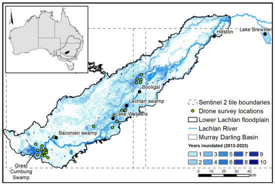
Figure 2.
The location of the lower Lachlan floodplain within the Murray–Darling Basin. The map shows the number of times the area was inundated over a 10-year period (July 2013–June 2023). The locations of the drone imagery sites are indicated by green circles.
The lower Lachlan floodplain was selected as the focus for this study because it encompasses a distributed network of floodplain wetlands with a dynamic range of vegetation types. This includes non-woody wetland vegetation (e.g., common reed, cumbungi), river red gum forests and woodlands, and flood-dependent shrublands such as lignum all with different inundation requirements [40]. The lower Lachlan floodplain is a highly regulated system with flows managed from Wyangala Dam in the upper Lachlan River Catchment. Environmental water management is used to mitigate the impacts of river regulation and altered flow regimes predominantly focusing on delivering water to the Great Cumbung Swamp and Booligal wetlands to support waterbird breeding and vegetation condition for habitat refuge (Figure 2).
Using the processed Sentinel-2 imagery, six indices were calculated (Table 1). These indices were selected as they are correlated with water and vegetation cover within pixels as well as soil and leaf moisture content.

Table 1.
List of indices used in AIM.
2.3. Ancillary Data Processing
In addition to water and vegetation indices, this method incorporates high-resolution digital elevation models (DEMs) to improve classification accuracy. We used the NSW state-wide LIDAR-derived DEM dataset at 5 m resolution captured during 2013, as well as a LIDAR-derived product collected at 1 m resolution in 2009 [45], covering parts of the Lachlan floodplains that partially overlap the mapping extent defined in Section 2.1. Processing the DEMs involved producing a downscaled DEM aligned with reflectance data for each Sentinel-2 tile being mapped. Each of the available DEMs covering a tile was clipped to that extent and downscaled to match the resolution and cell alignment of the Sentinel-2 10 m resolution bands. Where multiple DEM datasets overlapped, elevation information from the highest-resolution source DEM was retained in the final processed DEM.
Using the processed DEM, wetland depressions were delineated to facilitate the identification of inundated mixed and vegetation pixels. The rationale for this approach is that during the initial stages of flooding, these wetland depressions typically fill first and will retain water longer during flood recession, increasing their probability of inundation. Wetland depressions are created by first creating a probability of depression surface using the stochastic depression analysis tool in Whitebox Tools [46,47]. A threshold of 0.5 was applied to convert this into a binary map of depressions. Depressions were then evaluated with respect to multiple satellite images corresponding to moderate- and high-flow periods to manually remove incorrectly classified depressions.
An ancillary crop layer was generated to mask agricultural land use areas within the study region. The Felzenszwalb algorithm [48] was employed to segment Sentinel-2 NDVI time series imagery spanning the years 2022 to 2023. These segmented images were then integrated to create a composite image, highlighting landscape boundary probabilities. Rectangular crop boundaries were identified and extracted from the composite image. In cases where crop polygons exhibited irregular boundaries, manual extraction was performed by visually cross-referencing the vector polygons with satellite imagery obtained from DigitalGlobe within Google Earth Pro, version 7.3.6.9796 dated 13 August 2023.
2.4. Aerial Image Data Collection
Aerial images were collected from three different sources: aerial oblique photos and high-resolution airborne digital sensor imagery were used to identify thresholds, while drone capture of RGB imagery was performed for inundation extent validation purposes. Aerial surveys from a fixed-wing aircraft were conducted over the lower Lachlan floodplain on two occasions (18 January 2021 and 5 April 2023) to capture oblique photographs, which in complex areas were orthorectified (see Thomas et al. [30]). High-resolution RGB orthomosaics that covered part of the study area and obtained from aerial mounted Leica ADS40 sensors (Heerbrugg, Switzerland) were captured on 29 July 2020 and 5 April 2023. For each survey, photographed areas had 4241 points randomly generated and labelled with a binary inundation status (inundated/not inundated). As the purpose of this study was to classify inundated vegetation, each point was also labelled depending on whether the pixel it was in was dominated by vegetation cover or being sparsely covered (mostly non-vegetated). The labelling of features was undertaken by interpretation of the closest available Sentinel-2 image using the corresponding georeferenced aerial photographs to determine inundation and cover status. These data were collected and analysed to identify appropriate thresholds for classifying inundated from non-inundated (See Section 2.4). Drone imagery was captured during surveys conducted on the 20 April 2023 and 13 November 2023 to provide inundation extent validation data. There were 29 plots, each 500 m × 500 m, plots identified with 25 sites able to be mapped in each survey mission; surveys used a DJI Mavic-3E drone (Shenzhen, China) with an RGB sensor. Flights at each plot were conducted at 100 m altitude and a flight speed of 8.9 ms−1 with data from each plot orthorectified using Web OpenDroneMap, release version 2.5.0 [49]. We then classified areas of inundation and sparse cover (no vegetation present) in each plot using a combination of image classification and manual digitisation (see Supplementary Materials for details). A 10 m × 10 m grid was created over the sampled area and aligned to the Sentinel-2 pixels, and the percentage area inundated and vegetated for each pixel was calculated. Pixels with more than 10% inundated area detected were considered inundated. This low number threshold was used because partially inundated pixels are relevant to identifying where water is in the landscape, particularly in complex wetland areas with small, inundated features. In addition, this helps compensate for potential alignment errors between Sentinel-2 imagery and the drone images, for which this attempts to compensate.
2.5. Detecting Inundation Classes
2.5.1. Identifying Water
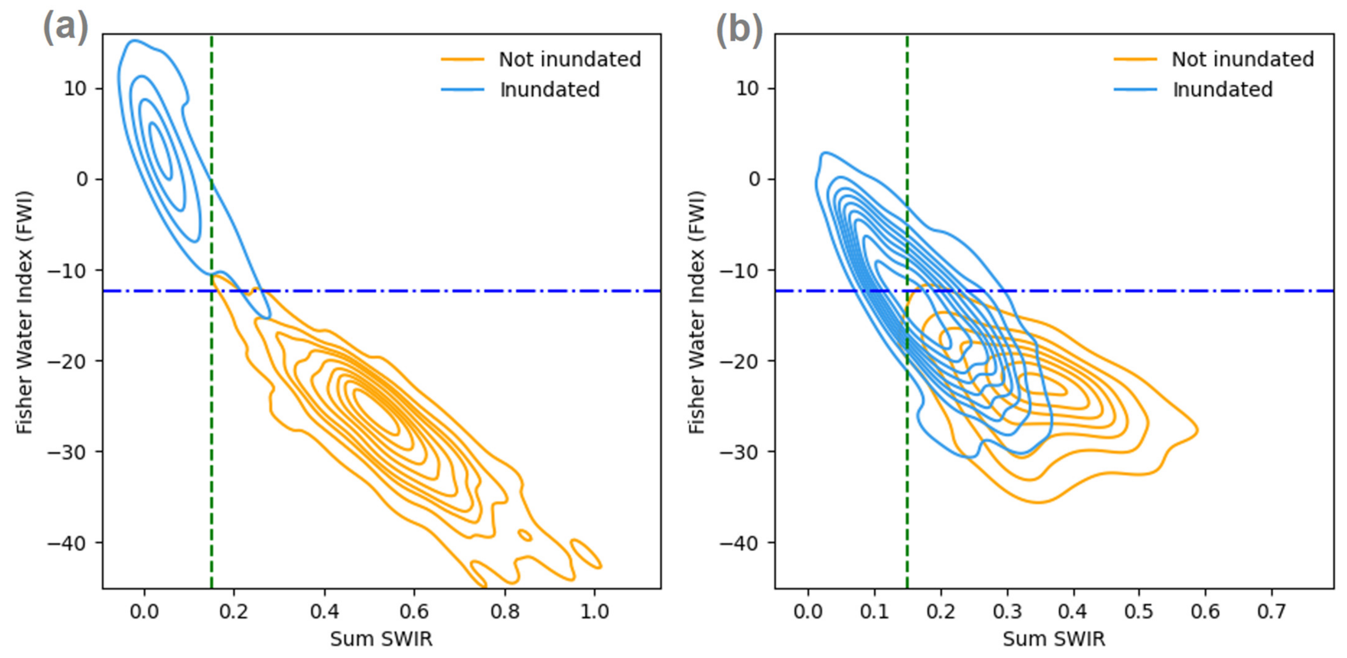
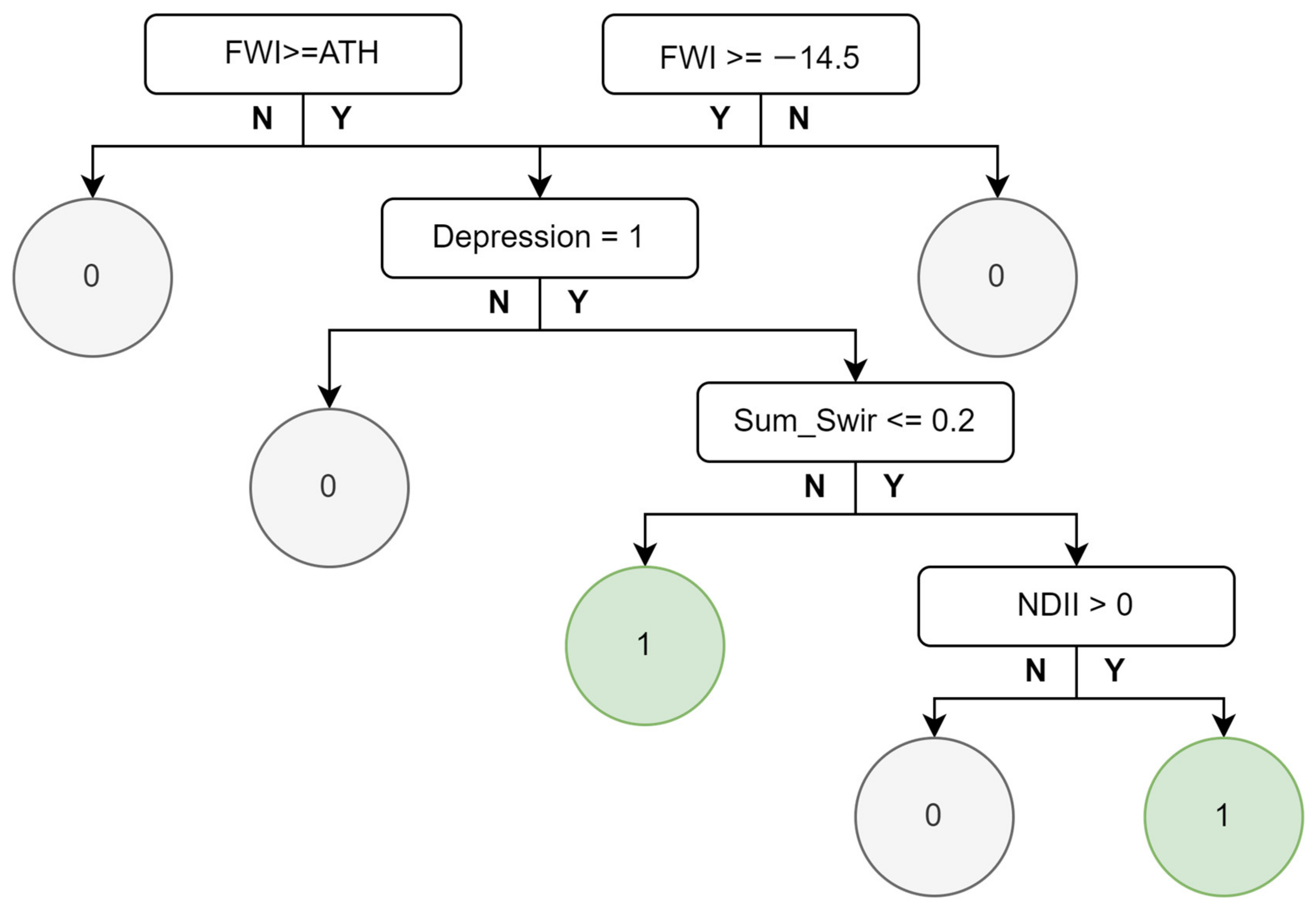
To identify open water, the Fisher water index (FWI; Fisher et al. [23]) was used. This approach has been demonstrated to perform well, and we found it manages mixed pixels better than other indices such as NDWI. The optimal threshold for identifying water identified by Fisher et al. [23] is 0.63. However, based on the analysis of Sentinel-2 images of the lower Lachlan catchment with oblique photographs collected from aerial surveys, we identified a threshold combination of FWI and Sum SWIR better suited for this region (Figure 3). Inundated areas are initially classified as pixels with FWI values ≥ −12.4 if total shortwave infrared reflectance (Sum SWIR) is lower than 0.15. If Sum SWIR is above this threshold, then the FWI threshold is still used, provided NDII is above 0.3 (Figure 4). A second condition is applied to consider pixels with FWI ≥ −11 as inundated if Sum SWIR values are less than 0.2 and NDII is above 0.1.
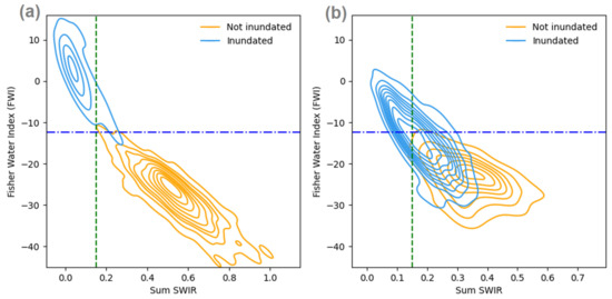
Figure 3.
Contour plots showing the density of observations at inundated and non-inundated sites under sparse cover pixels (a) and vegetated pixels (b) with selected thresholds for FWI and Sum SWIR indices.

Figure 4.
Decision tree outlining the conditions used to define water pixels.
The inclusion of Sum SWIR was considered because low infrared reflectance is a characteristic of the spectral response of water, while low shortwave infrared (SWIR) is characteristic of soil and vegetation with high moisture content [26,50]. NDII complements the Sum SWIR threshold as it is indicative of soil and vegetation moisture content [51,52]. The combination of these two constraints enables us to lower the FWI threshold to capture more water pixels that may be mixed with vegetation or soil. It also minimises potential commission error caused by lowering this threshold in non-inundated areas.
2.5.2. Identifying Mixed Pixels
Mixed pixels are areas that may contain water as well as other landcover types such as soil, living biomass (e.g., algae and growing vegetation) or non-living biomass (e.g., senescent vegetation and fallen timber). The previous step for identifying water (2.5.1) provides a secondary, relaxed FWI threshold to account for some mixed pixels. However, the lower Lachlan floodplain contains extensive areas with complex wetland features consisting of braided channels and small depressions containing dense vegetation. This results in mixed pixels that are difficult to identify as inundated. Examples of mixed and obscured inundated areas are shown in Figure 5.
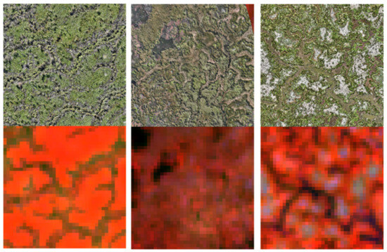
Figure 5.
Complex wetland features shown with 2.5 cm resolution RGB drone imagery (top row) and false-colour Sentinel-2 imagery (NIR -B8, SWIR2-B12, Red-B4). Each tile represents an area of 375 m × 375 m, with darker colours in Sentinel-2 imagery typically indicative of water. Column 1 shows inundated lignum-covered channels. Column 2 shows inundated dense reed beds with some open water. Column 3 shows an inundated depression complex with a mix of vegetation, water and bare earth. Red colours indicate vegetation, black areas are indicative of water and grey green areas are bare soil.
To overcome this, we combined mapped wetland depressions with FWI using a local adaptive threshold (ATH) approach. Local thresholds were obtained by calculating the weighted sum of values in a 21 × 21 pixel neighbourhood, with a Gaussian function determining the weights and applying a constant scaling factor of −8; this was implemented using OpenCV, version 4.8.0 [53]. To reduce the potential for commission errors, only pixels that were within a mapped wetland depression and had spectral characteristics suggestive of elevated moisture levels (either low Sum SWIR or elevated NDII) were considered as an inundated mixed pixel (Figure 6). We found that in woodland areas, this approach can misclassify tree shadows as mixed pixels. To mitigate this issue, we combined the areas detected as water and mixed pixels together and removed any mixed pixels that form isolated patches ≤ 3 pixels in size.
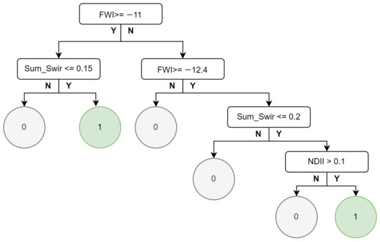
Figure 6.
Decision tree showing the conditions used to define mixed pixels.
2.5.3. Identifying Wetland Vegetation
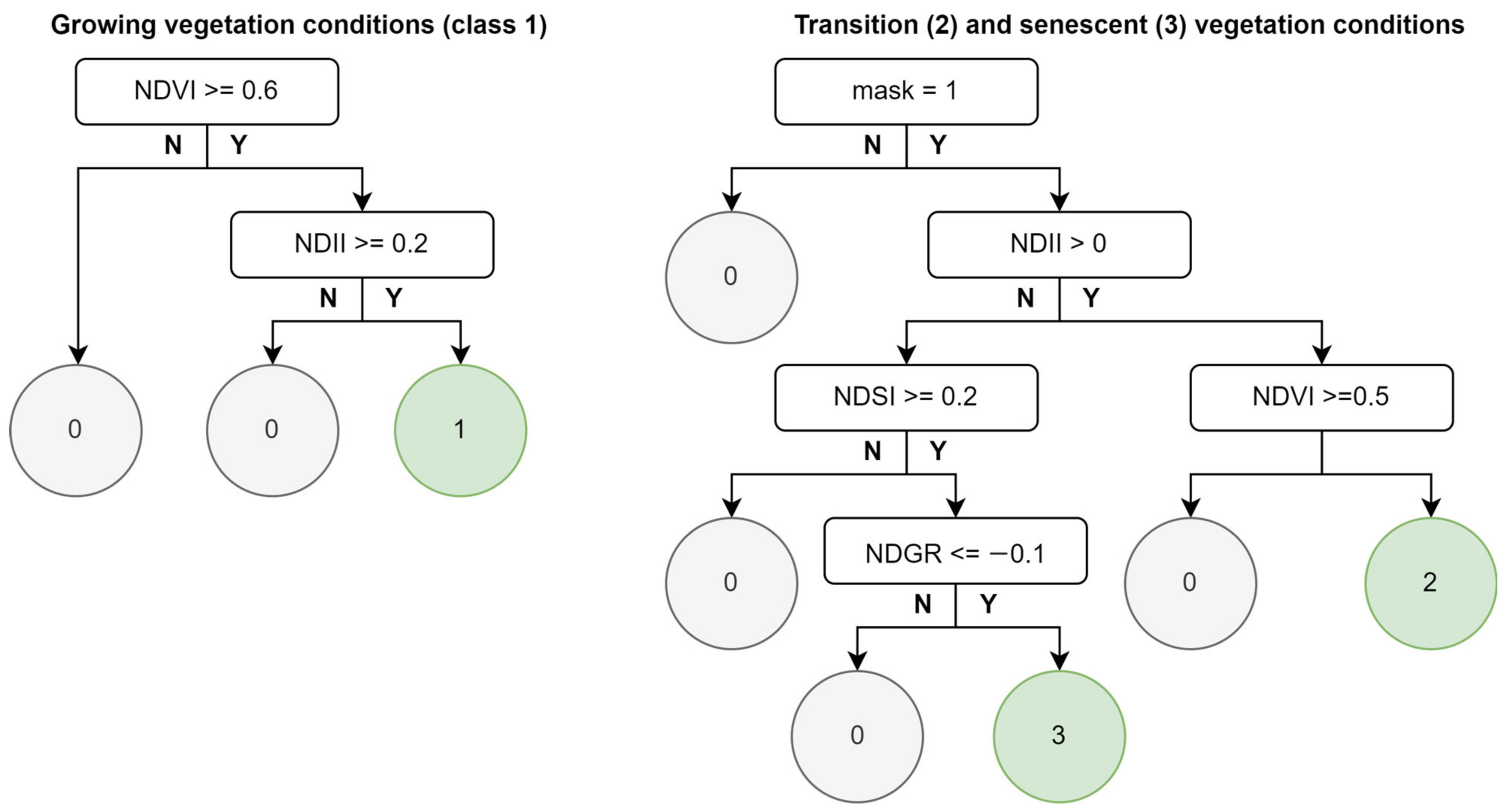
Detection of inundation in vegetation can be challenging, particularly where emergent vegetation is dense and the spectral signature of water is partially or completely obscured. Thomas et al. [36] utilised both NDVI and a form of the NDII to create a separate class for identifying both vigorously growing and senescent vegetation. We took a similar approach and prior to identifying inundated vegetation, focused on identifying healthy wetland vegetation with elevated moisture content. Wetland vegetation can include both woody and non-woody communities that have dynamic spectral signatures. These wetland communities can undergo significant changes in total biomass and species composition as they respond to moving in and out of dry and wet periods [54]. NDVI is an index that can be used to monitor wetland vegetation response to inundation, as the increase in moisture triggers vigorous growth, resulting in increased NDVI values and declining values as post-flood moisture leaves the system [55]. Analysis of wetland vegetation can be enhanced by including NDII as it enables the quantification of moisture content in addition to plant health [52,56]. In our approach, we classified wetland vegetation as having moderately high NDVI (>0.6) and NDII (>0.2) (Figure 7). We found this identified areas of vegetation that were either inundated, recently inundated or responding to elevated soil moisture due to heavy rainfall.
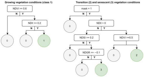
Figure 7.
Decision trees showing the conditions used to classify wetland vegetation.
This approach is adequate during the growing season and for vegetation types that do not undergo dormancy, where it is sufficient all year. However, some vegetation types such as water couch (Paspalum distichum) and common reed (Phragmites australis), gradually senesce from the peak of the growing period (March) to their dormancy period (June), with a rapid green up from mid-September to November. As vegetation transitions into and out of the senescent phase, NDII can be low due to decreasing leaf water content or the mixture of healthy new growth (high NDII) emerging from senescent plant material (low NDII).
To identify senescent wetland vegetation or wetland vegetation in transition (senescing or green up), we counted the frequency of pixels that were classified as wet vegetation during the previous growing season. This involved analysing the images with <30% cloud cover between November and February (inclusive). This frequency map was converted to a binary growing season mask (maskgrow), with frequencies greater than 3 assigned to a value of 1. Pixels will only be considered in transition or senescent if they were within this mask, as the wetland vegetation must have been present during the growing season for it to transition to a senescent state. Wetland vegetation in transition was determined as having moderate NDVI values and positive NDII values. The identification of senescent vegetation combined three indices to minimise the potential misclassification of bare soil as senescent vegetation. NDSI has been used previously to identify crop residue [43] and we found that values greater than 0.2 tend to be more indicative of senescent vegetation than soil in wetland areas in the lower Lachlan. We also found that senescent vegetation tends to have lower green reflectance relative to red reflectance (the inverse of healthy vegetation) with negative values of NDGR indicative of senescent vegetation. Finally, in senescent vegetation NDII will typically be negative, while wet soil is more likely to have positive values so the inclusion of NDII helps to avoid misclassification of wet soils. While there is overlap with soil in each of these indices, combining the indices with the growing season mask as defined in Figure 7 aims to reduce misclassification of soil.
2.5.4. Classifying Inundation Status of Wetland Vegetation
Determining the inundation status of vegetation is challenging as the spectral signature of water is obscured. In Section 2.5.3, we identify vegetated areas with high water content, which is indicative of vegetation that is inundated or growing in soils with high moisture content. Given the purpose of the AIM mapping product, it is important to infer whether these areas of wet vegetation are inundated. To carry this out, we used the DEM described in Section 2.5.3.
A binary mask is created where pixel values from water, mixed and vegetation processes are greater than zero. This mask represents the extent of wet areas (inundated areas and wetland vegetation). We then defined areas of inundation, which consisted of pixels classified as either water or mixed, as well as wetland vegetation covering the extent of a mapped depression, provided that the depression also contains water or mixed pixels. A focal analysis is then performed, calculating the maximum elevation of inundated pixels within a 21 × 21 pixel neighbourhood. The difference between the maximum local inundated height and the actual height is then calculated. Wetland vegetation that is above the local maximum inundation height was excluded from the wet area mask.
Regions of connected pixels of the updated wet area mask were treated as discrete objects, whose attributes were assessed to determine whether vegetation within those objects were inundated; objects that did not contain water or mixed pixels were removed from the mask. For each remaining object, we calculated the maximum height of vegetation pixels and inundated pixels. If the difference in elevation was small (<0.1 m) or the object was small (<50 pixels), the object was considered inundated. In larger objects, wet vegetation pixels with an elevation value less than the maximum height of inundated pixels within the object were considered inundated vegetation.
2.6. Final Map Assembly
Each of the processing steps defined previously results in the creation of four independent maps, which are combined to produce the final inundation map product. These maps are combined to create a full AIM map (AIMFULL) that maps all inundated and wetland classes (Equation (1)), which is then collapsed to form a simplified binary AIM map (AIMBIN, Equation (2)).
2.7. Evaluation
Inundation maps generated using the AIM process were generated from Sentinel-2 images coinciding with the drone surveys conducted during the weeks of the 20 April 2023 and 13 November 2023. For the April survey, the Sentinel-2 image was captured on 20 April 2023, while images available between 13–17 November 2023 were obscured by cloud, so we used the image collected on the 11 November 2023. Three plots in the 11 November 2023 image were partially obscured by cloud and were evaluated using the next available date, 6 November 2023. At other sites, while inundation extent was similar between dates, it was noted that water had receded slightly by 11 November 2023 and may result in higher commission errors at the three sites evaluated on 6 November 2023.
The binary inundation maps (AIMBIN) were then validated with the inundation status of pixels observed on the survey dates by calculating both user’s (also known as the true positive rate) and producer’s accuracy metrics (Table 2). User’s accuracy aims to quantify map accuracy from the perspective of the map user, describing the proportion of pixels classified as inundated that are truly inundated. Producer’s accuracy quantifies accuracy from the point of view of the map producer, and describes the what proportion of pixels that should be inundated are classified as inundated. In addition, we assessed overall accuracy as well as rates of omission and commission error (Table 2). This accuracy assessment was performed using empirical data from all survey plots to obtain a global estimate of classification accuracy, and was as reported for both vegetated and sparsely covered pixels separately. We presented an evaluation of these measures at the plot scale and assessed the effect of varying subpixel inundation percentages on classification accuracy. Finally, we provided two qualitative assessments of the AIM product. The first assessment involved a visual assessment of classified inundation maps used in the accuracy assessments to give context to the sources of both commission and omission errors. The second assessment was a case study, using AIM to map the planned delivery of environmental water to the Great Cumbung Swamp in December 2021.
Table 2.
Accuracy metrics used to evaluate inundation map. Metrics calculated from confusion matrix where TP = number of true positives, TN = number of true negatives, FP = number of false positives and FN = number of false negatives.
3. Results
3.1. Accuracy Assessment
The accuracy of the AIM product was assessed using data collected from 50 drone survey plots covering 1778 ha of the lower Lachlan River floodplain, with 40.5% of Sentinel-2 pixels surveyed inundated or partially inundated. At the study scale (all plots evaluated together), accuracy metrics were high, with overall and user’s accuracy measured at 0.87 and producer’s accuracy at 0.82. The slightly lower producer’s metric is attributable to higher omission error rate (0.18) compared to commission (0.13). Pixels were classified based on whether they were mostly vegetated (>50% vegetation cover) or sparsely covered (<50% vegetation) using the drone survey images; 61.3% of sparsely covered pixels were inundated compared to 29.7% of vegetated pixels. Overall accuracy was high for both sparse and vegetated cover types, with a very low commission error rate for sparsely covered pixels (4). However, producer’s and user’s metrics were much lower for vegetated pixels compared to those with sparse cover, which is attributable to both higher omission and commission rates (4). Despite this, overall accuracy remains comparable to sparsely covered pixels due to high specificity and a lower percentage of inundated vegetated pixels, resulting in a similar proportion of correctly classified pixels overall.
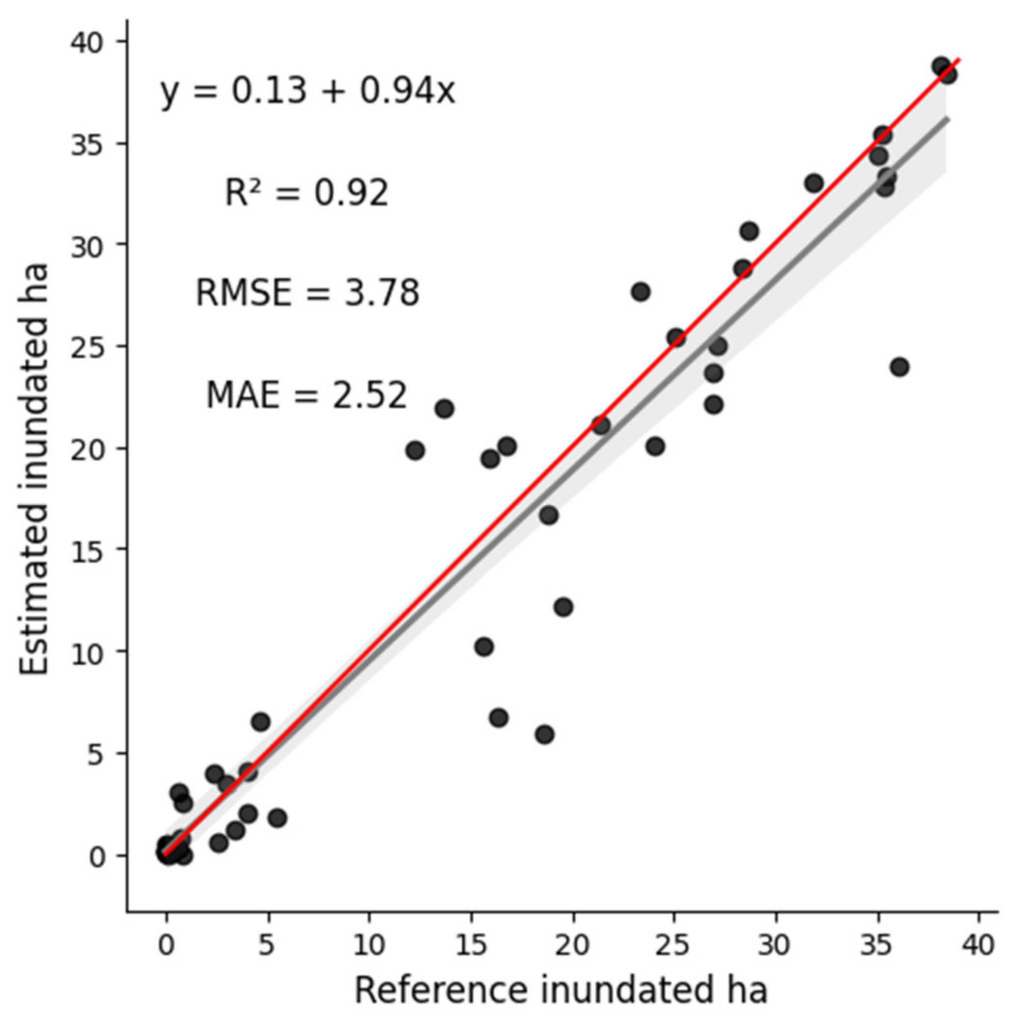
The AIM output was assessed at the plot scale by comparing reference inundation extents at each drone survey plot with the estimated inundation extent. The comparison, shown in Figure 8, demonstrates that inundation extent was slightly underestimated compared to the reference drone survey images, with a mean absolute error (MAE) of 2.5 ha and RMSE pf 3.8 ha. As seen in Figure 8, most surveys are centred near the trend line with a few distinct outliers. Removal of four sites with an absolute error greater than 8 ha reduces the MAE to 1.8 ha and RMSE to 2.6 ha. At three of these sites, omission of inundated areas was responsible for the large discrepancy to the reference inundated extent. The explanation of this discrepancy is discussed in the visual interpretation of results in Section 3.2.

Figure 8.
Relationship between reference inundated area from drone data and estimated inundation area from AIM at each survey plot (black points). The relationship is quantified by a linear regression model (grey line) with 95% confidence interval (grey shade) and the expected 1:1 relationship also shown (red line).
When assessing the accuracy metrics within each plot, overall accuracy and specificity remain high across all plots, while other accuracy metrics show considerable variability (Figure 9). The variability in producer’s and user’s accuracy is partially due to the proportion of the survey area that is inundated (Figure 10). Plots containing a low proportion of inundated pixels tend to accurately classify a high proportion of non-inundated (high specificity) while accurately classifying a lower number of inundated pixels (lower user’s accuracy values). The inverse is true for survey plots with a higher percentage of inundated pixels. This is likely because a large proportion of the minority class is mixed with the majority class (i.e., when a small number of inundated pixels surrounded by non-inundated pixels). The mixing of minority class pixels may mean they are spectrally similar to the adjacent majority class, resulting in a greater proportion of the minority class being misclassified. This results in a greater impact on omission and commission error rates, while overall accuracy remains consistent.
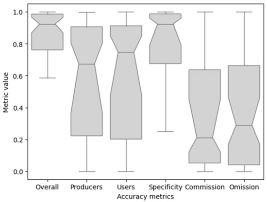
Figure 9.
Notched boxplots of accuracy metrics across all surveys. Centre lines show medians, with notches representing the bootstrapped 95% confidence interval.
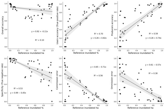
Figure 10.
Relationship between accuracy metrics (y-axis) and drone survey plot inundation percentage (x-axis).
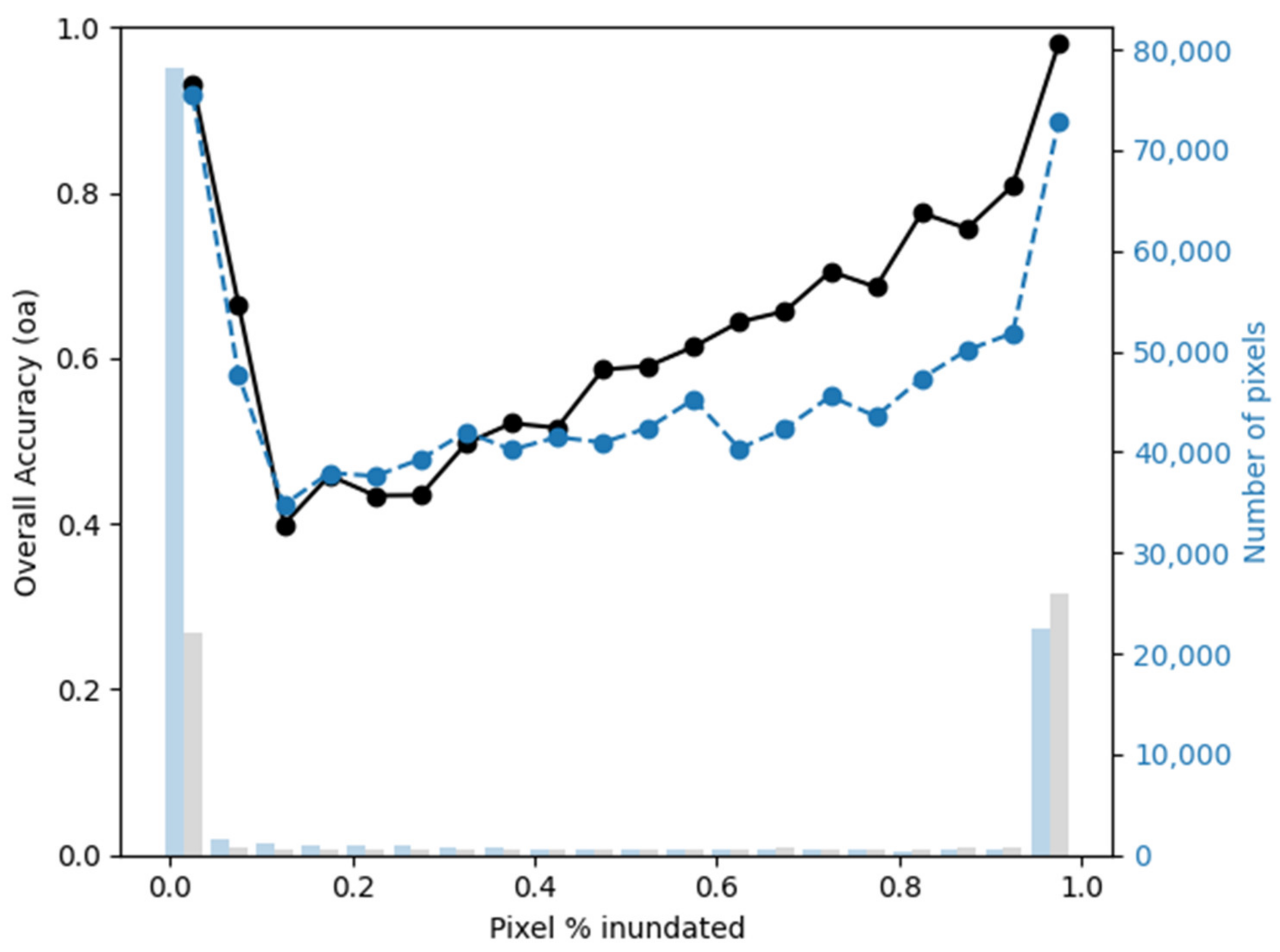
Accuracy was also measured at the subpixel level, where the percentage of inundated area within a Sentinel-2 image pixel was measured. The percentage inundation was grouped into 20 equal interval bins between 0 and 100%, and the overall accuracy of AIM was calculated within each bin. Pixels that were either completely inundated or not inundated had the highest overall accuracy for both sparse and vegetated pixels (Figure 11). Pixels with 15% inundation had the lowest overall accuracy, which increased linearly as percentage of inundation increased. Sample sizes between minimum and maximum bins were significantly smaller, as they represent pixels on the edge of inundated areas.

Figure 11.
Overall accuracy (black line) based on subpixel percentage inundation as measured from high-resolution drone data for sparse cover pixels (black) and vegetated pixels (blue). Data are calculated by binning inundation percent to equal interval categories. The number of pixels evaluated in each bin is shown in grey for sparse cover and light blue for vegetated cover.
3.2. Visual Assessment
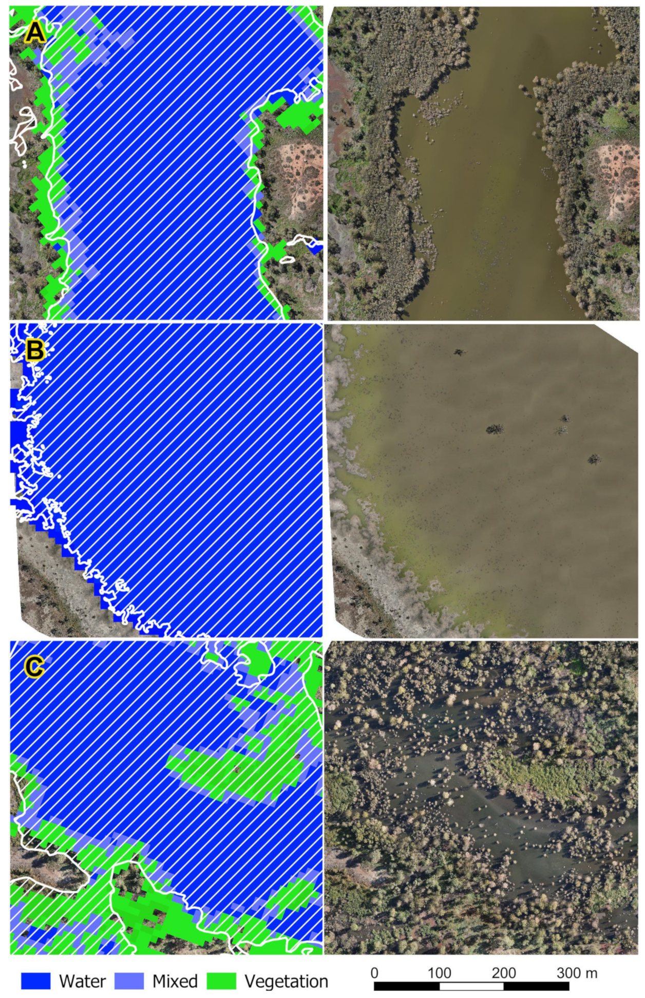
Visual assessment of results provides insights into where AIM performs well and why errors of commission and omission arise. Overall, the output of the AIM approach has a high degree of accuracy (Table 3). The areas where this approach performs best are large contiguous areas of inundation, such as open water bodies, or floodplain and wetland areas with a mosaic of open water and vegetated pixels (Figure 12). These features form a large proportion of the inundated area, and so likely contributed to high accuracy metrics.
Table 3.
Accuracy of AIM product over sparse and vegetated covered types. User’s accuracy is equivalent to the true positive rate (TPR), while specificity is the true negative rate (TNR).

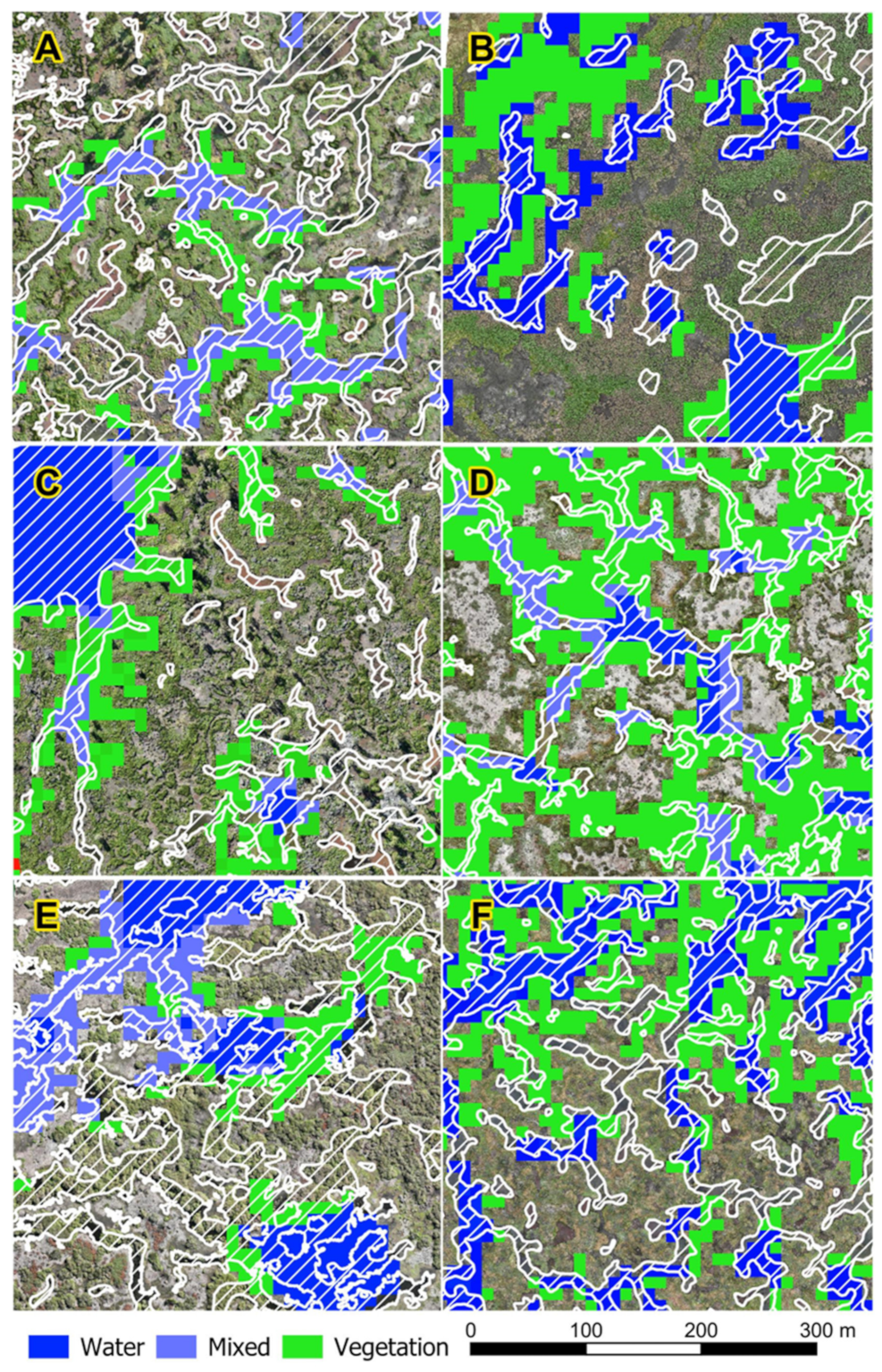
Figure 12.
Inundated features (white hatched polygons) over inundated classes from the AIM classification product and drone captured imagery as the underlying image. Rows (A–C) show different survey plots while raw drone imagery is shown in the right column for comparison. These are examples where AIM produced good results in landscapes containing larger inundated wetland features.
Omission errors contribute to an underestimate of inundation extent. A characteristic of Sentinel-2 products is the 10 m spatial resolution. In Figure 13A, the inundated area is dominated by small channels and depressions often less than 10 m wide. The AIM model has successfully classified channels >10 m in the middle of the image but has been unable to detect inundation in the large number of small, depressions elsewhere. This resulted in this plot having the greatest underestimated inundation extent of all surveys and therefore high errors of omission.
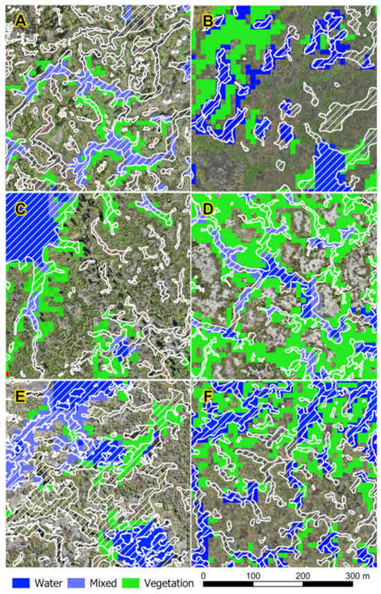
Figure 13.
Examples of inundated features (white hatched polygons) over inundated classes from the AIM classification product and drone captured imagery as the underlying image. These examples highlight areas of significant errors of omission (A,C,E) and commission (B,D,F).
Another source of omission error is where water is obscured by vegetation. The presence of lignum shrublands (Duma florulenta) presents challenges in the detection of inundation. In Figure 13E, there are several channels that are covered by lignum that are not classified as wet vegetation. This issue is evident in multiple sites where lignum is the dominant wetland vegetation type. Lignum is observed to have lower NDII values when inundated compared to other prevalent wetland vegetation types in the study area, such as common reed (Phragmites australis) and nardoo (Marsilea drummondii). This may be attributable to the leaf structure and growth form of lignum, which is a mass of tangled branches with thin linear leaves. Where wetland vegetation is detected by AIM, it can be misclassified as not inundated when it occurs in an unmapped depression or when there are large expanses of dense, inundated wetland vegetation. The latter issue was not found during the drone surveys but was observed when producing maps of major flooding events in the Great Cumbung Swamp during late 2022 (Figure 14). This is attributable to the neighbourhood operation that calculates the maximum height of nearby water pixels (See Section 2.5.4). With large expanses of vegetation, there are many areas with no open water visible within the range of the neighbourhood operation. This means our approach performs better when there is a matrix of open water and vegetation that enables the inference of inundation status of wetland vegetation. However, it is likely that many of the areas that could not be inferred as inundated in Figure 14 are inundated, given their location relative to surrounding mapped water pixels. These areas are classified as wetland vegetation in the AIMFULL output, meaning the classification could be revised post hoc. Further development work will aim to refine this automatically, and will require the collection of empirical validation data during conditions similar those seen in Figure 14 before incorporating this to ensure its validity.
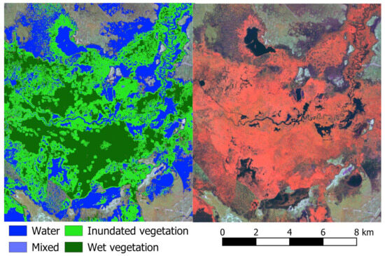
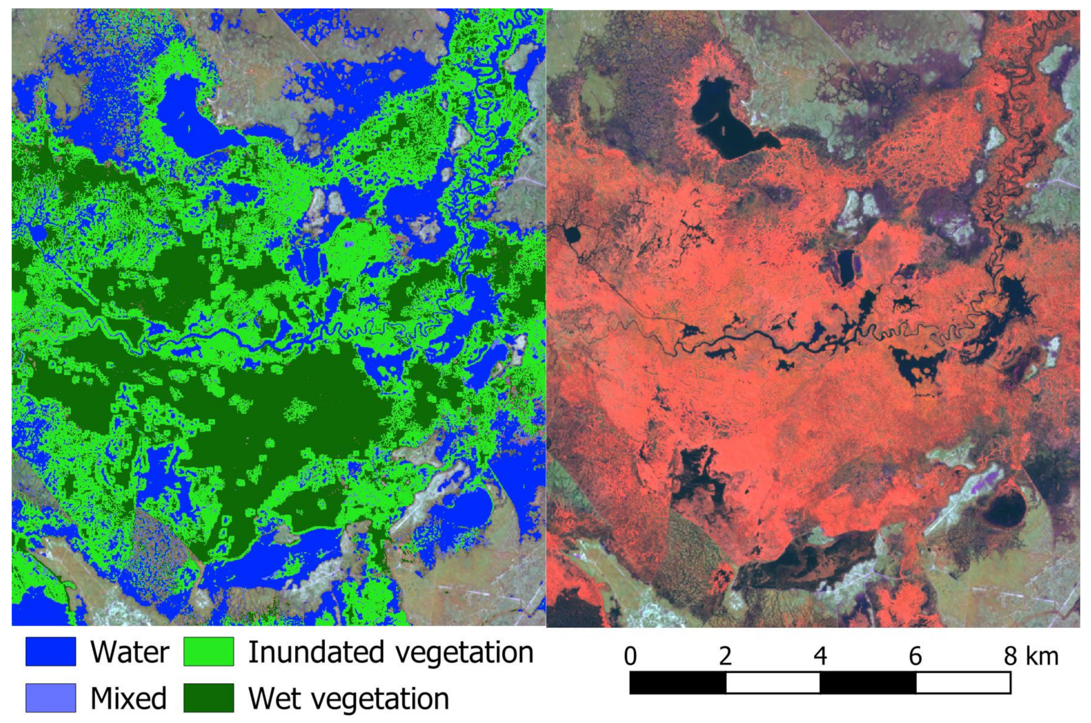
Figure 14.
A major flooding event in the Great Cumbung Swamp with AIM classification (left) and a Sentinel-2 satellite image captured on 17 October 2022 displayed in false colour (R = B8, G = B11, B = B4). This highlights the centre of the swamp, showing large contiguous areas of vegetation (red in the image displayed using the aforementioned false colour band combination) that is detected as wetland vegetation. The density of the vegetation hinders the detection of water in these areas, meaning the AIM method is unable to infer the inundation status of vegetation.
Commission errors overestimate inundation extent. These errors are higher for vegetated pixels relative to sparsely covered ones (Table 3). Examples of these errors can be seen in the right-hand column panels in Figure 13B,D,F. Misclassified inundated vegetation is often found adjacent to inundated depressions and channels that are identified as inundated. As the relief in these areas are low, these areas of vegetation have an elevation at or below the height of nearby water pixels.
While the likelihood of commission error is high for vegetated pixels (0.22, Table 3), many of these areas are close to inundated regions, have similar elevations, and were likely inundated previously, as these surveys were conducted during the recession from a large flood peak in December 2022. This means that while they may not be under surface water, they are remain influenced by the water from an inundation event. Therefore, the impact of these commission errors is lessened when using these maps compared to identifying inundated vegetation in areas that are not proximal to water and may never have been inundated.
Commission errors for sparsely vegetated pixels are low but still occur. We noted that in bare soils, where water has receded very recently, these areas can be detected as inundated. This was observed in one site in November, where water was receding exposing bare soil. The temporal lag between Sentinel-2 image capture (11th November) and drone survey (conducted on the week of the 13th November) may have meant some very shallow water was present in these areas during Sentinel-2 image capture and had receded by the time drone surveys were conducted (Figure 15).
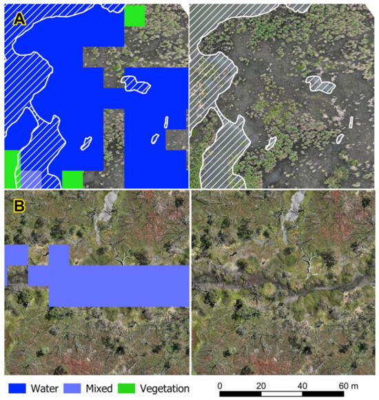
Figure 15.
Examples of typical commission errors seen in sparse covered areas for two drone survey sites (A,B). True inundated features (white hatched polygons) are shown over inundated classes from the AIM classification product and drone captured imagery as the underlying image.
A similar issue is observed from the mixed pixel process where mapped depressions with non-inundated wet soils are classified as inundated. This can be seen in Figure 15B, where the grey soils to the north of the image indicate dry conditions. In contrast, the moist, dark and partially vegetated channel through the middle suggests higher moisture levels. The moist soils in the mapped depressions are likely contributing to high FWI relative to adjacent dry areas, resulting in them being detected by the adaptive threshold of the mixed pixel process.
3.3. Case Study of Environmental Flow Event
3.3.1. Overview of the Flow Event
In 2020 over a 27-day period (28 August to 17 September 2020), over 129,500 megalitres (ML) of translucent flows passed Lake Brewster Weir, upstream of Hillston (Figure 16). Translucent flows are a type of planned environmental water that is delivered according to a set of rules by the river operator (WaterNSW). Environmental water managers have no decision-making role over the translucent flow regime or resultant lateral connectivity with the floodplain. However, they can add great value by delivering additional water to extend the duration of connectivity between the Lachlan River and floodplain wetlands.
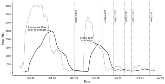
Figure 16.
River flow data obtained from Water NSW (www.realtimedata.waternsw.com.au, accessed on 12 June 2024) at Hillston weir (grey) and Booligal (black) with translucent and environmental flow (e-flow) pulses labelled. Vertical dashed lines show dates mapped using AIM.
This was the intent of the 2020 post-translucent environmental water delivery, and managers were targeting the Lachlan Swamp below Booligal and Great Cumbung Swamp, the terminus wetland of the Lachlan River Catchment (Figure 1 and Figure 17). The delivery started at Lake Brewster Weir after translucent flows on 18 September 2020 and continued until 2 November 2020 at Booligal Weir (Figure 16). This pulse was observed moving through the Lachlan swamps area above Lake Waljeers, near Booligal on the 11 December 2020 (Figure 17, box A).
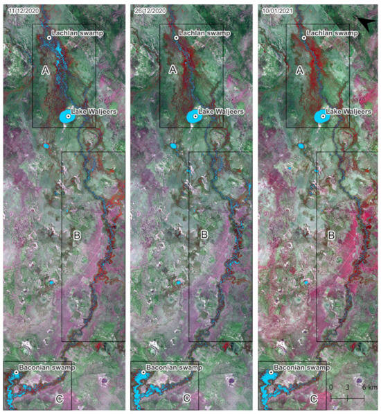
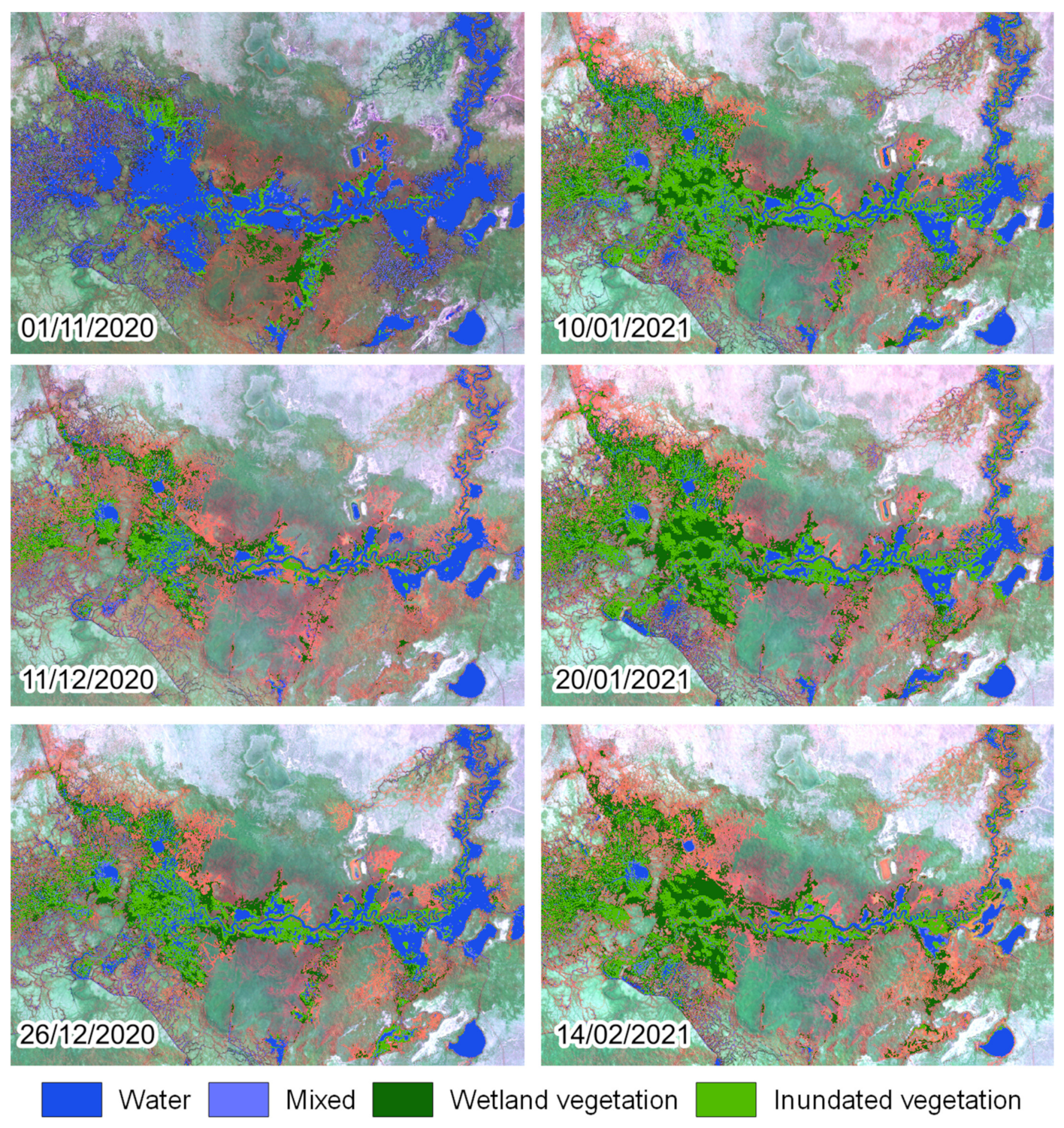
Figure 17.
Time series showing the progression of inundation from environmental water delivery down the lower Lachlan River between 11 December 2020–10 December 2021. Light-blue colours indicate areas detected as inundated using AIM. Box A highlights the area above Lake Waljeers, while box C highlights the Baconian Swamp that is upstream from the Great Cumbung Swamp. Box B highlights the area between these two regions.
By the 26 December most of this water has drained from the area while the inundation extent has increased downstream (Figure 17, Box B, C). By 10 January 2021, the remaining environmental water below Lake Waljeers had receded (Figure 17, Box B) with inundation extent in the Baconian Swamp, upstream from the Great Cumbung Swamp remaining high (Figure 17, Box C).
As explained previously, the translucent flow provided the important initial inundation of the Great Cumbung Swamp, observed arriving around 1 November 2020, which had largely receded by 11 December 2020 (Figure 18). On 26 November, the additional targeted 2020 post-translucent environmental water delivery was observed filling the area, with inundation extent remaining high between 10 to 20 January 2021. By 14 February 2021, the environmental water had begun receding (Figure 18). The mapping highlighted the success of the strategy to use discretionary environmental water after translucent flows to extend the duration and depth of inundation for several months. This is key to ensuring the critical life cycle requirements for ecosystem functions, such as waterbird and frog breeding, vegetation seed setting, and recruitment are completed.

Figure 18.
Time series of observations showing the fluctuation of inundation extent in the Great Cumbung Swamp due to natural and environmental water delivery.
3.3.2. Evaluation of Map Performance
The inundation maps generated using the AIM approach have successfully produced maps characterised the inundation dynamics of the Great Cumbung Swamp. The natural flow in November 2020 resulted in the landscape being largely dominated by open water, which has stimulated significant vegetation growth in the following dates. This made detection of water via the water and mixed processes (Section 2.5.1 and Section 2) impossible, highlighting the importance of inundated vegetation processes (Section 2.5.3 and Section 4) for capturing the dynamics in this area. While we do not have ground truth data to quantitatively validate the accuracy of all these maps, there are aerial oblique photographs for the map created for 20 January 2021 that was used to evaluate thresholds. Overall accuracy for this date was measured at 0.9, with a low commission error rate (0.06) and moderate omission error rate (0.19). This date is also shows the maximum inundation extent identified, and preceding dates do not show inundated pixels outside the inundated area identified on the 20 January 2021, suggesting that commission errors likely remain low in these other dates.
In the images for 10 January 2021 and 20 January 2021, there are large patches of wetland vegetation within the inundated vegetation class. This has occurred because the emergent vegetation has obscured the detection of water and mixed pixels. Therefore, when the focal analysis is performed during the inundated vegetation process (Section 2.5.4), there are no nearby water pixels available to obtain the maximum inundation height. As a result, these areas are potentially excluded from being classified as inundated.
Another challenging feature to map are the small braided channels to the northeast and southwest areas. The full extent of inundated channels was not captured by the AIM output but the inclusion of the mixed pixel process has enabled the capture of more of these features.
In summary, AIM method effectively capture most of the impact of environmental water delivery into the Lachlan Swamp and Great Cumbung Swamp. However, the full extent of inundated vegetation may be underestimated in some areas and fine scale features such as small channels may not be fully captured.
4. Discussion
Many wetlands, including those found in the lower Lachlan floodplain, are characterised by a range of hydromorphological attributes [57,58] and diverse vegetation communities [15], where species composition and total biomass can vary significantly depending on inundation dynamics [54]. This variability presents challenges to inundation mapping with consideration of the spectral responses of vegetation and to the ability to detect the presence of water throughout both wetting and drying cycles of the system is required [54,59]. The classification and mapping approach presented here attempts to overcome these challenges by combining FWI, Sum SWIR and NDII using two separate processes that adopt both fixed and locally adaptive thresholds to identify open water and mixed water pixels. This approach also leverages mapped wetland depressions from high-resolution DEMs to enable and improve the capture of small wetland features. The final component of the model incorporates the combination of NDVI, NDII and NDSI to identify wetland vegetation with inundation status inferred using high resolution DEM.
Other methods that have been used to map water in the MDB have focused primarily on open surface water [27,31] with the detection of inundated vegetation much more challenging due to the inability of water indices alone to detect inundation of dense emergent vegetation. Ticehurst et al. [27] attempted to improve inundation detection across different landscapes using multiple indices derived from 30 m Landsat data with land classification layers used to apply the optimal index and threshold. This approach managed to improve classification accuracy in vegetated wetlands but still resulted in errors of omission in densely vegetated areas. In comparison, we employ four classification processes using Sentinel-2 imagery to identify water, mixed pixels in wetland depressions and wetland vegetation, finally utilising elevation and proximity to classify inundation status of the vegetation. In this regard, our approach may provide more detail on the inundation status within the lower Lachlan floodplain, although no direct comparison was made here. This is because our use of higher-resolution imagery and a multi-process approach to classifying inundation enables us to better capture complex wetland features that are prevalent in the lower Lachlan. This includes the ability to capture inundation within the Cumbung Swamp which often has a dense cover of common reed (Phragmites australis), particularly in wet years. However, our approach does not have the temporal extent of these other products as Sentinel-2 did not launch until 2015, meaning no Sentinel-2 images are available prior to late 2016.
Overall, the AIM approach works well in detecting water across the wetlands with high overall accuracy (Table 3) but still encountered some limitations. We found inundated wetland features that are comparable in size or smaller than the resolution of the Sentinel-2 imagery has a higher likelihood of not being detected, although the mixed pixel process implemented ensured we detected more of these features than if we relied on the water detection process alone. In addition, we found the classification of inundation status of vegetation has a higher degree of uncertainty compared to sparsely covered areas, in particular open water bodies which are detected accurately. Drone surveys were conducted during a period of recession after major flooding and overestimation of inundated vegetation is likely attributable to the persistence of moist soils and low variation of elevation. In the dates surveyed, wet vegetation is widely detected while water is typically found within depressions but the lack of difference in measured elevation between water pixels and wet vegetation results in their classification as inundated. While we aim to be able to identify inundation status accurately for each individual date, these errors or commission are less significant than if dry areas were identified as inundated. This is because these areas were likely recently inundated, contain high soil moisture content (under the influence of water in the environment) and are connected to water bodies making them potentially important areas for wetland fauna. The opposite issue was also identified when evaluating peak flow periods in October 2022, where inundation status was unable to be inferred as water pixels were unable to be detected within expansive stands of dense reeds within the Great Cumbung Swamp. Again, while this type of omission error is not ideal, these areas are detected as wet vegetation which can be reclassified post-hoc and forms the basis for continued work to identify a process to incorporate into AIM to improve classification in this scenario.
Other limitations of our approach relate to the incorporation of elevation data and its derivatives. AIM requires the availability of accurate DEMs to detect the inundation status of complex wetland features as well as dense vegetation. The availability of high resolution DEMs are spatially variable with 1 m DEMs available in the southern portion of the study area, while NSW Statewide 5 m DEMs were used where higher resolution ones were not available. This meant the accuracy of depression delineation and inference of inundation status of vegetation was also spatially variable and could lead to bias and the propagation of errors over time. However, the most accurate DEMs were available in the most complex and most likely to be inundated wetland region (Great Cumbung Swamp) so it is likely this has not had a significant negative effect on measured accuracies. This product is also dependent on the delineation of wetland areas likely to be covered by water-dependent vegetation to ensure water within senescent vegetated is detected. This enables AIM to estimate inundation extent of vegetation outside of the growing season but as with the depression layer, can introduce error if not created accurately.
As previously mentioned, the outputs of AIM detected the presence of water across complex, vegetated floodplain wetlands of the lower Lachlan. However, there is still uncertainty in the detection of inundation, particularly the inundation status of vegetation in certain situations. To account for this uncertainty and produce a product that presents a more complete picture of the extent of water in the environment the AIM approach also classifies wet vegetation that we can assume to be either inundated or vegetation within wet soil. This opens up the application of AIM maps to the assessment of wetland vegetation where above and below ground surface water may be important for vegetation growth and condition. Given the complexity of the landscape in the lower Lachlan system, the AIM mapping product should be transferable to other floodplain wetlands of the MDB but further research is required. Having the AIM mapping product available will allow key decisions in relation to environmental water delivery to be made to ensure that the Environmental Water Requirements (EWR) are being met in each wetland. This is supported by our case study (Section 3.3), which indicated that water delivery had made it to an inlet channel to Lake Bullogal, a high-priority target. If the mapping had been available, it would have given managers confidence to consider modifying the watering action and ordering additional water to specifically target Lake Bullogal. In hindsight, the mapping will be invaluable for planning future events in terms of understanding the relationship between the commence-to-flow (CTF) height and duration for optimal flooding of Lachlan Swamp.
With regard to the derived datasets used in AIM (depressions, crop masks), we acknowledge that the initialisation of these datasets is not an automated process. This may limit user willingness to trial this approach. However, users can trial AIM by omitting the conditions that require depressions in the decision trees described in Figure 4 and Figure 6. This will reduce the upfront initialisation cost at the expense of increased commission error of automatically generated inundation maps. Alternative methods incorporating DEMs are available that may have a lower upfront initialisation cost. Psomiadis et al. [60] use a 5 m DEM to create a flood elevation surface by interpolating elevation values at the edge of the inundation extent estimated by remote sensing indices. They then expand the inundation extent to nearby areas that are lower in elevation. However, this approach still requires the delineation of barriers to water flows such as levies, which they incorporate into their interpolation process. There also needs to be consideration for the temporal dynamics of flood events. As flood waters expand, areas of low elevation near flood water may not be inundated as water has not yet reached that location. This is one reason why we constrain our approach to only consider wet areas when inferring inundating status of vegetation to prevent this type of error. Another consideration is that in patches of dense vegetation water is often only visible in the deepest points within the patch. Extrapolation in this scenario is challenging as other parts of the vegetated patch is likely of higher elevation. Due to this issue, we consider wetland vegetation in mapped depressions as inundated when there is visible water. This highlights why the mapping of wetland depressions is an important step to initialise AIM. Improvement of methods for the creation of these derived datasets required to maintain the accuracy of AIM is ongoing. Other work that we are undertaking to further develop AIM is the transferability of the method in other wetlands. Additional data are being collected in other wetlands in the MDB to sample a broader range of soil and vegetation types in different seasons to validate and refine our approach.
5. Conclusions
The AIM mapping approach can be used to detect inundation across complex vegetation systems of the lower Lachlan floodplain. By incorporating several indices, depression layers and wetland boundaries, the model was able to distinguish water in open water bodies and under dense vegetation groups. This approach enables the mapping of both the extent of inundated areas and wet areas, providing a more complete picture of water in the environment. Although further research needs to be conducted in other wetland floodplains of the MDB, this AIM mapping product should be transferable with slight modifications made. Developing the AIM mapping product to monitor wetland floodplains across the MDB will strongly influence decisions made in relation to environmental water management.
Supplementary Materials
The following supporting information can be downloaded at: https://www.mdpi.com/article/10.3390/rs16132434/s1. The supplementary material published online alongside the manuscript provides details about the drone image classification, inundation classification and cover classification. An example of issues encountered when classifying inundation status of drone imagery is provided using Figure S1: Examples of issues encountered classifying inundation status of drone imagery. Includes specular reflection (A), inundated forests (B), dense non-woody vegetation (C) and an example of high-resolution DEM of the same extent shown in C (D).
Author Contributions
Conceptualization, J.T.H. and R.F.T.; methodology, J.T.H., L.G., T.G., R.F.T. and J.L.; software, J.T.H., L.G. and T.G.; validation, L.G. and J.T.H.; formal analysis, L.G.; investigation, L.G.; resources, J.T.H. and L.G.; data curation, J.T.H., L.G. and T.G.; writing—original draft preparation, J.T.H., L.G., T.G., R.F.T. and J.L.; writing—review and editing, J.T.H., L.G., T.G., R.F.T. and J.L.; visualization, J.T.H., L.G. and T.G.; supervision, J.T.H., R.F.T. and J.L.; project administration, J.T.H.; funding acquisition, R.F.T. All authors have read and agreed to the published version of the manuscript.
Funding
This research was financially supported by the NSW Department of Climate Change, Energy, the Environment and Water as part of the Water for the Environment program and by the Australian Government’s Federal Funding Agreement.
Data Availability Statement
Data are currently only available on request and can be shared via online platforms. Please email lead author for any data request.
Acknowledgments
We acknowledge the traditional custodians of the lands where we live. We thank the many landholders across the lower Lachlan wetlands for supporting our field surveys by providing access to their properties. Field surveys would not have been possible without many dedicated personnel, and so we thank those who supported the field data collected over the study period.
Conflicts of Interest
The authors declare no conflict of interest.
References
- Ling, J.E.; Casanova, M.T.; Shannon, I.; Powell, M. Development of a wetland plant indicator list to inform the delineation of wetlands in New South Wales. Mar. Freshw. Res. 2019, 70, 322–344. [Google Scholar] [CrossRef]
- New South Wales, Department of Climate Change, Energy, the Environment and Water. NSW Wetlands Policy. DECCW; 2010. Available online: https://www.environment.nsw.gov.au/topics/water/wetlands/protecting-wetlands/nsw-wetlands-policy (accessed on 29 April 2024).
- Casanova, M.T.; Brock, M.A. How do depth, duration and frequency of flooding influence the establishment of wetland plant communities? Plant Ecol. 2000, 147, 237–250. [Google Scholar] [CrossRef]
- Ocock, J.F.; Walcott, A.; Spencer, J.; Karunaratne, S.; Thomas, R.F.; Heath, J.T.; Preston, D. Managing flows for frogs: Wetland inundation extent and duration promote wetland-dependent amphibian breeding success. Mar. Freshw. Res. 2024, 75, MF23181. [Google Scholar] [CrossRef]
- Brandis, K.; Bino, G.; Spencer, J.; Ramp, D.; Kingsford, R. Decline in colonial waterbird breeding highlights loss of Ramsar wetland function. Biol. Conserv. 2018, 225, 22–30. [Google Scholar] [CrossRef]
- Pander, J.; Mueller, M.; Geist, J. Habitat diversity and connectivity govern the conservation value of restored aquatic floodplain habitats. Biol. Conserv. 2018, 217, 1–10. [Google Scholar] [CrossRef]
- Frazier, P.; Page, K. The effect of river regulation on floodplain wetland inundation, Murrumbidgee River, Australia. Mar. Freshw. Res. 2006, 57, 133–141. [Google Scholar] [CrossRef]
- Virkki, V.; Alanärä, E.; Porkka, M.; Ahopelto, L.; Gleeson, T.; Mohan, C.; Wang-Erlandsson, L.; Flörke, M.; Gerten, D.; Gosling, S.N.; et al. Globally widespread and increasing violations of environmental flow envelopes. Hydrol. Earth Syst. Sci. 2022, 26, 3315–3336. [Google Scholar] [CrossRef]
- Kingsford, R.T.; Basset, A.; Jackson, L. Wetlands: Conservation’s poor cousins. Aquat. Conserv. Mar. Freshw. Ecosyst. 2016, 26, 892–916. [Google Scholar] [CrossRef]
- Tickner, D.; Opperman, J.J.; Abell, R.; Acreman, M.; Arthington, A.H.; Bunn, S.E.; Cooke, S.J.; Dalton, J.; Darwall, W.; Edwards, G.; et al. Bending the Curve of Global Freshwater Biodiversity Loss: An Emergency Recovery Plan. Bioscience 2020, 70, 330–342. [Google Scholar] [CrossRef]
- Chen, Y.; Colloff, M.J.; Lukasiewicz, A.; Pittock, J. A trickle, not a flood: Environmental watering in the Murray–Darling Basin, Australia. Mar. Freshw. Res. 2021, 72, 601–619. [Google Scholar] [CrossRef]
- Department of Planning and Environment. NSW Long Term Water Plans: Background Information; Department of Planning and Environment: Parramatta, Australia, 2023. [Google Scholar]
- Sheldon, F.; Rocheta, E.; Steinfeld, C.; Colloff, M.; Moggridge, B.J.; Carmody, E.; Hillman, T.; Kingsford, R.T.; Pittock, J. Testing the achievement of environmental water requirements in the Murray-Darling Basin, Australia. Preprints 2023. [Google Scholar] [CrossRef]
- Higgisson, W.; Cobb, A.; Tschierschke, A.; Dyer, F. The Role of Environmental Water and Reedbed Condition on the Response of Phragmites australis Reedbeds to Flooding. Remote Sens. 2022, 14, 1868. [Google Scholar] [CrossRef]
- Higgisson, W.; Higgisson, B.; Powell, M.; Driver, P.; Dyer, F. Impacts of water resource development on hydrological connectivity of different floodplain habitats in a highly variable system. River Res. Appl. 2020, 36, 542–552. [Google Scholar] [CrossRef]
- Thomas, R.F.; Ocock, J.F. Macquarie Marshes: Murray-Darling River Basin (Australia). In The Wetland Book; Finlayson, C., Milton, G., Prentice, R., Davidson, N., Eds.; Springer: Dordrecht, The Netherlands, 2016. [Google Scholar] [CrossRef]
- Thomas, R.F.; Kingsford, R.T.; Lu, Y.; Hunter, S.J. Landsat mapping of annual inundation (1979–2006) of the Macquarie Marshes in semi-arid Australia. Int. J. Remote Sens. 2011, 32, 4545–4569. [Google Scholar] [CrossRef]
- Burke, J.J.; Pricope, N.G.; Blum, J. Thermal imagery-derived surface inundation modeling to assess flood risk in a flood-pulsed savannah watershed in Botswana and Namibia. Remote Sens. 2016, 8, 676. [Google Scholar] [CrossRef]
- Tiwari, V.; Kumar, V.; Matin, M.A.; Thapa, A.; Ellenburg, W.L.; Gupta, N.; Thapa, S. Flood inundation mapping-Kerala 2018; Harnessing the power of SAR, automatic threshold detection method and Google Earth Engine. PLoS ONE 2020, 15, e0237324. [Google Scholar] [CrossRef] [PubMed]
- Kordelas, G.A.; Manakos, I.; Aragonés, D.; Díaz-Delgado, R.; Bustamante, J. Fast and automatic data-driven thresholding for inundation mapping with Sentinel-2 data. Remote Sens. 2018, 10, 910. [Google Scholar] [CrossRef]
- Shen, X.; Wang, D.; Mao, K.; Anagnostou, E.; Hong, Y. Inundation extent mapping by synthetic aperture radar: A review. Remote Sens. 2019, 11, 879. [Google Scholar] [CrossRef]
- Drusch, M.; Del Bello, U.; Carlier, S.; Colin, O.; Fernandez, V.; Gascon, F.; Hoersch, B.; Isola, C.; Laberinti, P.; Bargellini, P.; et al. Sentinel-2: ESA’s optical high-resolution mission for GMES operational services. Remote Sens. Environ. 2012, 120, 25–36. [Google Scholar] [CrossRef]
- Fisher, A.; Flood, N.; Danaher, T. Comparing Landsat water index methods for automated water classification in eastern Australia. Remote Sens. Environ. 2016, 175, 167–182. [Google Scholar] [CrossRef]
- Xu, H. Modification of normalised difference water index (NDWI) to enhance open water features in remotely sensed imagery. Int. J. Remote Sens. 2006, 27, 3025–3033. [Google Scholar] [CrossRef]
- McFeeters, S.K. The use of the Normalized Difference Water Index (NDWI) in the delineation of open water features. Int. J. Remote Sens. 1996, 17, 1425–1432. [Google Scholar] [CrossRef]
- Lefebvre, G.; Davranche, A.; Willm, L.; Campagna, J.; Redmond, L.; Merle, C.; Guelmami, A.; Poulin, B. Introducing WIW for Detecting the Presence of Water in Wetlands with Landsat and Sentinel Satellites. Remote Sens. 2019, 11, 2210. [Google Scholar] [CrossRef]
- Ticehurst, C.; Teng, J.; Sengupta, A. Development of a Multi-Index Method Based on Landsat Reflectance Data to Map Open Water in a Complex Environment. Remote Sens. 2022, 14, 1158. [Google Scholar] [CrossRef]
- Kordelas, G.A.; Manakos, I.; Lefebvre, G.; Poulin, B. Automatic inundation mapping using sentinel-2 data applicable to both camargue and do’ana biosphere reserves. Remote Sens. 2019, 11, 2251. [Google Scholar] [CrossRef]
- Senanayake, I.P.; Yeo, I.-Y.; Kuczera, G.A. A Random Forest-Based Multi-Index Classification (RaFMIC) Approach to Mapping Three-Decadal Inundation Dynamics in Dryland Wetlands Using Google Earth Engine. Remote Sens. 2023, 15, 1263. [Google Scholar] [CrossRef]
- Tulbure, M.G.; Broich, M.; Stehman, S.V.; Kommareddy, A. Surface water extent dynamics from three decades of seasonally continuous Landsat time series at subcontinental scale in a semi-arid region. Remote Sens. Environ. 2016, 178, 142–157. [Google Scholar] [CrossRef]
- Mueller, N.; Lewis, A.; Roberts, D.; Ring, S.; Melrose, R.; Sixsmith, J.; Lymburner, L.; McIntyre, A.; Tan, P.; Curnow, S.; et al. Water observations from space: Mapping surface water from 25 years of Landsat imagery across Australia. Remote Sens. Environ. 2016, 174, 341–352. [Google Scholar] [CrossRef]
- Dunn, B.; Lymburner, L.; Newey, V.; Hicks, A.; Carey, H. Developing a Tool for Wetland Characterization Using Fractional Cover, Tasseled Cap Wetness and Water Observations from Space. In Proceedings of the IGARSS 2019—2019 IEEE International Geoscience and Remote Sensing Symposium, Yokohama, Japan, 28 July–2 August 2019; pp. 6095–6097. [Google Scholar]
- Lymburner, L.; Sixsmith, J.; Lewis, A.; Purss, M. Fractional Cover (FC25). Geoscience Australia Dataset 2014. Available online: https://pid.geoscience.gov.au/dataset/ga/79676 (accessed on 29 April 2024).
- Ticehurst, C.J.; Teng, J.; Sengupta, A. Generating two-monthly surface water images for the Murray-Darling Basin. In Proceedings of the MODSIM2021, 24th International Congress on Modelling and Simulation, Sydney, Australia, 5–9 December 2021. [Google Scholar]
- Ma, S.; Zhou, Y.; Gowda, P.H.; Dong, J.; Zhang, G.; Kakani, V.G.; Wagle, P.; Chen, L.; Flynn, K.C.; Jiang, W. Application of the water-related spectral reflectance indices: A review. Ecol. Indic. 2019, 98, 68–79. [Google Scholar] [CrossRef]
- Thomas, R.F.; Kingsford, R.T.; Lu, Y.; Cox, S.J.; Sims, N.C.; Hunter, S.J. Mapping inundation in the heterogeneous floodplain wetlands of the Macquarie Marshes, using Landsat Thematic Mapper. J. Hydrol. 2015, 524, 194–213. [Google Scholar] [CrossRef]
- Flood, N.; Danaher, T.; Gill, T.; Gillingham, S. An Operational Scheme for Deriving Standardised Surface Reflectance from Landsat TM/ETM+ and SPOT HRG Imagery for Eastern Australia. Remote Sens. 2013, 5, 83–109. [Google Scholar] [CrossRef]
- Farr, T.G.; Rosen, P.A.; Caro, E.; Crippen, R.; Duren, R.; Hensley, S.; Kobrick, M.; Paller, M.; Rodriguez, E.; Roth, L.; et al. The Shuttle Radar Topography Mission. Rev. Geophys. 2007, 45. [Google Scholar] [CrossRef]
- Gallant, J.; Read, A. Enhancing the SRTM data for Australia. Proc. Geomorphometry 2009, 31, 149–154. [Google Scholar]
- Green, D.; Petrovic, J.; Burrell, M.; Moss, P. Water Resources and Management Overview: Lachlan Catchment; NSW Office of Water: Sydney, Australia, 2011. [Google Scholar]
- Tucker, C.J. Red and photographic infrared linear combinations for monitoring vegetation. Remote Sens. Environ. 1979, 8, 127–150. [Google Scholar] [CrossRef]
- Klemas, V.; Smart, R. The influence of soil salinity, growth form, and leaf moisture on the spectral radiance of Spartina Alterniflora canopies. Photogramm. Eng. Remote Sens 1983, 49, 77–83. [Google Scholar]
- Van Deventer, A.; Ward, A.D.; Gowda, P.H.; Lyon, J.G. Using thematic mapper data to identify contrasting soil plains and tillage practices. Photogramm. Eng. Remote Sens. 1997, 63, 87–93. [Google Scholar]
- Motohka, T.; Nasahara, K.N.; Oguma, H.; Tsuchida, S. Applicability of Green-Red Vegetation Index for Remote Sensing of Vegetation Phenology. Remote Sens. 2010, 2, 2369–2387. [Google Scholar] [CrossRef]
- Geoscience Australia. Digital Elevation Model (DEM) of Australia Derived from LiDAR 5 Metre Grid. Canberra, 2015. Available online: https://ecat.ga.gov.au/geonetwork/srv/eng/catalog.search#/metadata/89644 (accessed on 29 April 2024).
- Lindsay, J. The whitebox geospatial analysis tools project and open-access GIS. In Proceedings of the GIS Research UK 22nd Annual Conference, Glasgow, UK, 16–18 April 2014. [Google Scholar]
- Lindsay, J.B.; Creed, I.F. Distinguishing actual and artefact depressions in digital elevation data. Comput. Geosci. 2006, 32, 1192–1204. [Google Scholar] [CrossRef]
- Felzenszwalb, P.F.; Huttenlocher, D.P. Efficient Graph-Based Image Segmentation. Int. J. Comput. Vis. 2004, 59, 167–181. [Google Scholar] [CrossRef]
- OpenDroneMap. OpenDroneMap Documentation. 2020. Available online: https://docs.opendronemap.org/ (accessed on 29 April 2024).
- Mahdavi, S.; Salehi, B.; Granger, J.; Amani, M.; Brisco, B.; Huang, W. Remote sensing for wetland classification: A comprehensive review. GIScience Remote Sens. 2018, 55, 623–658. [Google Scholar] [CrossRef]
- Chen, D.; Huang, J.; Jackson, T.J. Vegetation water content estimation for corn and soybeans using spectral indices derived from MODIS near-and short-wave infrared bands. Remote Sens. Environ. 2005, 98, 225–236. [Google Scholar] [CrossRef]
- Joiner, J.; Yoshida, Y.; Anderson, M.; Holmes, T.; Hain, C.; Reichle, R.; Koster, R.; Middleton, E.; Zeng, F.-W. Global relationships among traditional reflectance vegetation indices (NDVI and NDII), evapotranspiration (ET), and soil moisture variability on weekly timescales. Remote Sens Env. 2018, 219, 339–352. [Google Scholar] [CrossRef] [PubMed]
- Bradski, G. The openCV library. Dr. Dobb’s J. Softw. Tools Prof. Program. 2000, 25, 120–123. [Google Scholar]
- Colloff, M.J.; Baldwin, D.S. Resilience of floodplain ecosystems in a semi-arid environment. Rangel. J. 2010, 32, 305–314. [Google Scholar] [CrossRef]
- Powell, S.J.; Jakeman, A.; Croke, B. Can NDVI response indicate the effective flood extent in macrophyte dominated floodplain wetlands? Ecol. Indic. 2014, 45, 486–493. [Google Scholar] [CrossRef]
- Wilson, N.R.; Norman, L.M. Analysis of vegetation recovery surrounding a restored wetland using the normalized difference infrared index (NDII) and normalized difference vegetation index (NDVI). Int. J. Remote Sens. 2018, 39, 3243–3274. [Google Scholar] [CrossRef]
- Lisenby, P.E.; Tooth, S.; Ralph, T.J. Product vs. process? The role of geomorphology in wetland characterization. Sci. Total Environ. 2019, 663, 980–991. [Google Scholar] [CrossRef]
- Semeniuk, C.; Semeniuk, V. A Comprehensive Classification of Inland Wetlands of Western Australia Using the Geomorphic-Hydrologic Approach; Royal Society of Western Australia: Karawara, Australia, 2016; Volume 94, pp. 449–464. [Google Scholar]
- Thapa, R.; Thoms, M.; Parsons, M. An adaptive cycle hypothesis of semi-arid floodplain vegetation productivity in dry and wet resource states. Ecohydrology 2016, 9, 39–51. [Google Scholar] [CrossRef]
- Psomiadis, E.; Soulis, K.X.; Zoka, M.; Dercas, N. Synergistic Approach of Remote Sensing and GIS Techniques for Flash-Flood Monitoring and Damage Assessment in Thessaly Plain Area, Greece. Water 2019, 11, 448. [Google Scholar] [CrossRef]


Disclaimer/Publisher’s Note: The statements, opinions and data contained in all publications are solely those of the individual author(s) and contributor(s) and not of MDPI and/or the editor(s). MDPI and/or the editor(s) disclaim responsibility for any injury to people or property resulting from any ideas, methods, instructions or products referred to in the content. |
© 2024 by the authors. Licensee MDPI, Basel, Switzerland. This article is an open access article distributed under the terms and conditions of the Creative Commons Attribution (CC BY) license (https://creativecommons.org/licenses/by/4.0/).