Abstract
Segmenting clouds and their shadows is a critical challenge in remote sensing image processing. The shape, texture, lighting conditions, and background of clouds and their shadows impact the effectiveness of cloud detection. Currently, architectures that maintain high resolution throughout the entire information-extraction process are rapidly emerging. This parallel architecture, combining high and low resolutions, produces detailed high-resolution representations, enhancing segmentation prediction accuracy. This paper continues the parallel architecture of high and low resolution. When handling high- and low-resolution images, this paper employs a hybrid approach combining the Transformer and CNN models. This method facilitates interaction between the two models, enabling the extraction of both semantic and spatial details from the images. To address the challenge of inadequate fusion and significant information loss between high- and low-resolution images, this paper introduces a method based on ASMA (Axial Sharing Mixed Attention). This approach establishes pixel-level dependencies between high-resolution and low-resolution images, aiming to enhance the efficiency of image fusion. In addition, to enhance the effective focus on critical information in remote sensing images, the AGM (Attention Guide Module) is introduced, to integrate attention elements from original features into ASMA, to alleviate the problem of insufficient channel modeling of the self-attention mechanism. Our experimental results on the Cloud and Cloud Shadow dataset, the SPARCS dataset, and the CSWV dataset demonstrate the effectiveness of our method, surpassing the state-of-the-art techniques for cloud and cloud shadow segmentation.
1. Introduction
Cloud segmentation and cloud shadow segmentation are crucial in remote sensing, meteorology, environmental monitoring, and other fields. Cloud coverage is closely related to environmental changes, such as global warming and climate change. By monitoring cloud coverage and cloud shadow, we can better understand the trend and impact of environmental changes [1,2]. Natural disasters, such as floods and forest fires, may be obscured by cloud cover, thus affecting monitoring and assessment [3]. Cloud segmentation and cloud shadow segmentation can help identify affected areas and guide rescue and emergency response work. Accurate segmentation of clouds and cloud shadows is also crucial for scientific research, resource management and planning, and land cover classification.
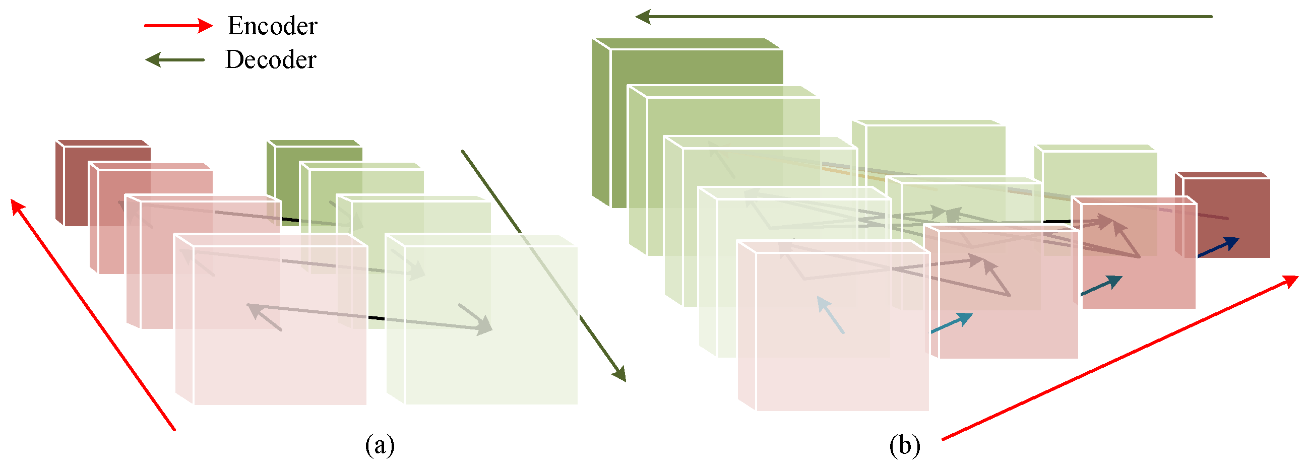
In the existing models for processing segmentation tasks, most networks are based on the UNet [4] architecture. As illustrated in Figure 1a, the network primarily consists of an encoding stage and a decoding stage. During the encoding phase, the convolution or transformer method is usually used, to extract features from high resolution to low resolution. In the decoding phase, there are multiple direct connections linking the encoder and the decoder. These connections facilitate the direct transfer of feature maps from each encoder layer to its corresponding layer in the decoder, aiding in the restoration of high-resolution details and enhancing the segmentation effectiveness. In addition, dilated convolution [5] and pooling operations [6] are utilized to expand the encoder’s receptive field for deep information.
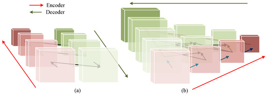
Figure 1.
Comparison diagram of network architecture. (a) UNet network architecture. (b) HRNet network architecture.
Our network adopts a similar architecture to that of HRNet [7]. As shown in Figure 1b, unlike the UNet architecture, which reduces image resolution in the encoding phase and restores image resolution in the decoding phase, our network maintains a high-resolution representation throughout the entire process of extracting information, and it simultaneously processes high-resolution and low-resolution features through multi-scale branches. Multi-resolution features are continuously merged throughout the network, to retain more detailed information. Since the design always retains high-resolution features, our network performs better in processing high-resolution images and is more suitable for the task of fine segmentation of clouds and cloud shadows.
It is well-known that Transformers can model long-distance dependencies and capture global feature information in images [8,9]. To address the CNN model’s limitations in global modeling [10,11], we integrate the Swin Transformer with the CNN model during feature extraction. Equal amounts of CNN and Transformer sub-modules are added at the same feature extraction stage. The interaction between the CNN model and the Transformer model enables the extraction of detailed and spatial features separately. Within the same feature extraction stage, it effectively combines fine and coarse, high-resolution and low-resolution features, establishing an information interaction platform between the Transformer and the CNN.
In HRNet, splicing or addition is employed as the fusion method within the same feature extraction stage. The fusion fails to effectively adjust the weight distribution of features and suppress the influence of unimportant features, which causes information redundancy. Moreover, simple fusion methods fail to capture dependencies between features, hindering the model’s ability to perceive global information. In the latest multi-scale feature fusion research, Yin [12] frequently used addition and splicing when performing differential information fusion. Lee [13] introduced MPvit, which splices fine and coarse features from Transformer and CNN at the same feature level. Xu [14] proposed PIDNet, which uses Bag Model to connect the difference information of three branches. In some recent cloud detection studies, Chen [6] used Transformer to interact information between a CNN encoder and decoder and used pooling to enhance the deep features of the encoder. Using a CNN-based architecture, Dai [15] also used multi-scale pooling to enhance the information of the encoder’s deep features but used Location Attention to help effectively repair the features. However, these methods use splicing when dealing with feature fusion, which is not conducive to information interaction between features. This paper proposes a novel fusion method using attention mechanisms. Features with different scale information are introduced into ASMA, where the dependence between positions is analyzed pixel-by-pixel through interactive fusion of axial attention, leading to the reconstruction of features at different scales. Additionally, the attention mechanism [16,17,18,19] captures relationships and contextual information across spatial dimensions in the image. Its main goal is to model long-distance dependencies and enhance feature expression capabilities. It ignores the information interaction and feature expression capabilities between channels. Therefore, this paper adds Channel Attention to the AGM, to guide ASMA to better complete image pixel-level reconstruction. Through AGASMA (Attention Guide Axial Sharing Mixed Attention), the spatial and channel dimension information between multi-scale features is better integrated. In summary, this paper uses AGASMA to better integrate the multi-scale information provided by the CNN and the Transformer in the same feature extraction stage, and builds an interactive platform between the CNN and the Transformer, which provides a more effective solution for cloud detection tasks. The key contributions of this paper include the following:
- We have developed a network that preserves high resolution throughout the entire process for cloud and cloud shadow segmentation. We have adopted a method of parallel-connecting sub-networks from high to low scales, to maintain high-resolution features throughout the entire process. The network is capable of achieving high-quality cloud detection tasks.
- The parallel-connected Transformer and CNN sub-models create a platform for interaction between fine and coarse features at the same level. This approach mitigates the limitations of using the Transformer and CNN models separately, enhances the acquisition of semantic and detailed information, and improves the model’s ability to accurately locate and segment clouds and cloud shadows.
- Most polymerization of high and low resolutions use splicing and addition operations. On the contrary, we use ASMA to obtain the dependence of the spatial position of pixels in high-resolution images and low-resolution images, which effectively aggregates multi-scale information, mitigating issues such as difficult image positioning and unclear boundaries caused by information loss. Additionally, incorporating the AGM enhances the modeling capability of the self-attention channel, enhancing the integration of high- and low-resolution channels and spatial features.
2. Related Work
2.1. Cloud Detection
Traditional cloud detection usually uses a threshold method for detection [20,21,22], which segments the image based on the pixel value thresholds. Cloud pixels often have different brightness or color, so clouds and ground can be separated by selecting the appropriate threshold. However, the threshold method typically requires manual selection of an appropriate threshold to segment cloud and non-cloud areas in an image. This approach is highly dependent on manual parameter selection, while the shape, size, thickness, and color of clouds are highly variable. The traditional threshold method may not perform well in dealing with these complex weather and geomorphic conditions.
There are many difficulties and challenges in cloud detection tasks. Clouds and their shadows exhibit diverse shapes and structures, with complex textures that heighten detection complexity. Furthermore, varying lighting conditions and weather fluctuations can disrupt accurate cloud segmentation [23]. Similar colors and features among categories—such as clouds and snow, cloud shadows and water, and cloud shadows and dark ridges within the same image—add further complexity to cloud detection [24].
Nowadays, the method of deep learning provides a new idea for cloud detection [25,26,27,28]. Mohajerani [29] used the FCN (Fully Convolutional neural Network) to extract the characteristics of clouds, which can realize the segmentation of clouds of different sizes [30]. However, the straightforward splicing method used in the upsampling process led to significant loss of detailed information. Chen [31] proposed the ACDNet. This model can have good results in complex scenes, such as the coexistence of clouds and snow, and large interference. However, when there are thin clouds and clouds and snow in the scene at the same time, the large-scale missed detection and false detection of the model still exist. Zhang [32] proposed the MTDR-Net for high-resolution remote sensing cloud segmentation and snow segmentation tasks. The network exhibited strong capabilities for anti-interference, cloud boundary refinement, and thin cloud extraction. However, Zhang did not conduct further research on effectively fusing high and low resolutions. Dai [15] used multi-scale pooling and attention to achieve fine cloud detection. The aforementioned research relied on cloud detection using CNN models. CNNs are typically constrained by the size of their convolutional windows during feature extraction, resulting in a relatively fixed receptive field. While CNNs excel in extracting detailed information, they often lack comprehensive understanding of the semantic structure of the entire image. However, the Transformer can consider the semantic association between different positions of the whole image in a serialized way. In the actual cloud detection task, the semantic association between positions can be used to detect the segmentation between similar objects, such as the segmentation between cloud and snow, or between cloud shadow and water. Chen [33] proposed the DBNet by combining the CNN and the CVT [34]. The DBNet effectively utilizes the complementary advantages of the Transformer and the CNN to efficiently complete cloud detection tasks. However, the CVT integrates convolution into Transformer. Although it effectively alleviates the problem of the insufficient local information extraction of the Transformer model, it greatly increases the computational complexity. Additionally, the DBNet employs a straightforward concatenation operation for fusing the CNN and the Transformer features, which limits the effective integration of local and global information. Guo [35] proposed MMA, which integrates CNN and Transformer information within the same feature extraction stage, achieving precise segmentation of clouds and cloud shadows in complex backgrounds. However, MMA also faces the challenge of using a simplistic concatenation approach.
2.2. Remote Sensing Image Processing
In recent years, DCNNs (Deep Convolutional Neural Networks) have made remarkable breakthroughs in computer vision, significantly advancing various image processing tasks. The research starting point in this field can be traced back to some previous methods based on the CNN [36,37,38,39,40,41]. DCNNs perform well in image classification tasks and lay a solid foundation for pixel-level classification tasks. Despite the significant progress of DCNNs in handling image tasks, they still encounter challenges, particularly in capturing long-range dependencies. Although some methods alleviate this problem by extending the receptive field, they still cannot fully capture the global features [42]. In practical applications, we aim for models to comprehensively assess the entire image context, prioritize key information, and accurately perceive pixel correlations. Since pixels in images typically exhibit interdependencies, they often display varying degrees of correlation. Therefore, although methods like global average pooling [37] help the model capture the overall average of the feature map, they may not fully emphasize critical regions.
Here, the Transformer model [8,43] effectively alleviates the occurrence of such problems. The success of the Transformer model provides a new research idea for global dependency modeling. The Transformer, originally prominent in natural language processing, has made a significant impact since its introduction into the field of computer vision. Among these advancements, Carion et al. [44] introduced the DETR model, which employs the Transformer’s encoder–decoder architecture to model interactions among sequence elements. Similar to earlier CNN-based models, Chen et al. [19] devised a dual-branch Transformer architecture to capture feature representations across various scales. The findings indicate that multi-scale feature representation is beneficial for visual Transformer models, such as ViT [34,45]. Based on this idea, the Swin Transformer [46] came into being, which constructs a new Transformer structure and shows great potential in multiple intensive prediction tasks. In particular, models utilizing the Swin Transformer have shown significant advancements in medical image segmentation [47,48]. In remote sensing image processing, several Swin Transformer-based models [49] have also demonstrated promising results. Recently, the fusion of the Transformer and the CNN has introduced a novel research direction in remote sensing image processing [33,50,51,52]. This combination leverages the long-distance dependency capabilities of Transformer models and the local modeling strengths of the CNN, offering a modeling approach for the model discussed in this paper.
2.3. Multi-Scale Fusion
It is common to use multi-scale Backbone to change from high resolution to low resolution through multiple sub-networks. Finally, using the UNet architecture [53], the skip connection aids in incrementally recovering features from lower to higher resolutions, and low semantic information is merged into high semantic information. The commonly used method of parallel multi-scale is to use a similar scheme to PPM [37] and ASPP [5]. At the same feature level, the same feature is convolved into high-to-low features, which are then stitched or added together through image restoration operations, such as deconvolution. HRNet combines series multi-scale with parallel multi-scale, and it maintains high resolution throughout the process, making it very friendly towards intensive prediction tasks: this paper drew some inspiration from this scheme.
2.4. Attention
In the process of information fusion, self-attention functions as a mechanism for spatial region and channel selection [54,55]. Fu [56] introduced the DANet (Dual Attention Network), which utilizes a self-attention mechanism to capture feature dependencies across spatial and channel dimensions. It consists of two parallel attention modules: the PAM (Position Attention Module), which captures dependency relationships between any two positions in the feature map, and the CAM (Channel Attention Module), which captures dependency relationships between any two channels. However, the amount of calculation required is large and the time cost is large. Huang [17] proposed the CCNet (Criss-Cross attention for semantic segmentation), to address issues such as memory consumption and excessive computation caused by self-attention. By employing stacked axial attention across two dimensions, it mitigates the problem of computational complexity, to some extent, but it causes too much loss of multi-scale information during exchange, and it cannot effectively establish the dependence between different-scale image pixels. In this paper, AGASMA is inspired by the above model, to some extent.
3. Methodology
3.1. Network Structure
This paper proposes a high-resolution multi-scale model that spans the entire process. The structure primarily consists of parallel cross-connections between CNN and Swin Transformer sub-networks. Multi-scale is used in both parallel and serial dimensions, respectively. This multi-scale architecture effectively enables accurate identification of clouds and cloud shadows. The parallel structure of the CNN and the Transformer facilitates the generation of both detailed and coarse feature representations at the same hierarchical level, thereby achieving precise localization and fine segmentation of clouds and cloud shadows. This approach aids in establishing dependencies between pixels at both long distances and locally. To effectively integrate parallel multi-scale information and address the issue of multi-scale positioning of clouds and cloud shadows, this paper introduces the ASMA method. Unlike the simple information fusion of different scales in models like [57,58], ASMA establishes pixel-level dependencies across resolution images of varying scales. The application of SMA (Sharing Mixed Attention) alleviates the problem that the axial attention is limited to the window size in capturing information to a certain extent. The Cloud and Cloud Shadow dataset exhibits significant noise levels. To enhance the model’s resistance to interference and to improve ASMA’s ability to integrate high- and low-resolution features across spatial and channel dimensions, this study employed the AGM to guide ASMA and to augment the model’s channel-space modeling ability. Figure 2 illustrates the high-resolution multi-scale model, while Figure 3 and Figure 4 detail specific modules within Figure 2. Table 1 provides detailed information on the feature extraction module used.
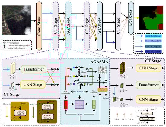
Figure 2.
High-resolution network overall architecture diagram. ‘Conv Stage’ represents the preparation stage of high-resolution image extraction, and ‘CNN Stage’ represents the convolution stage sub-network.’Transformer’ represents the Transformer-stage sub-network. ‘AGASMA’ represents the Attention Guide Axial Sharing Mixed Attention module. ‘Attention’ represents the Attention Guide Module. ‘Softmax’ is the activation function.
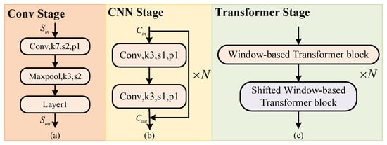
Figure 3.
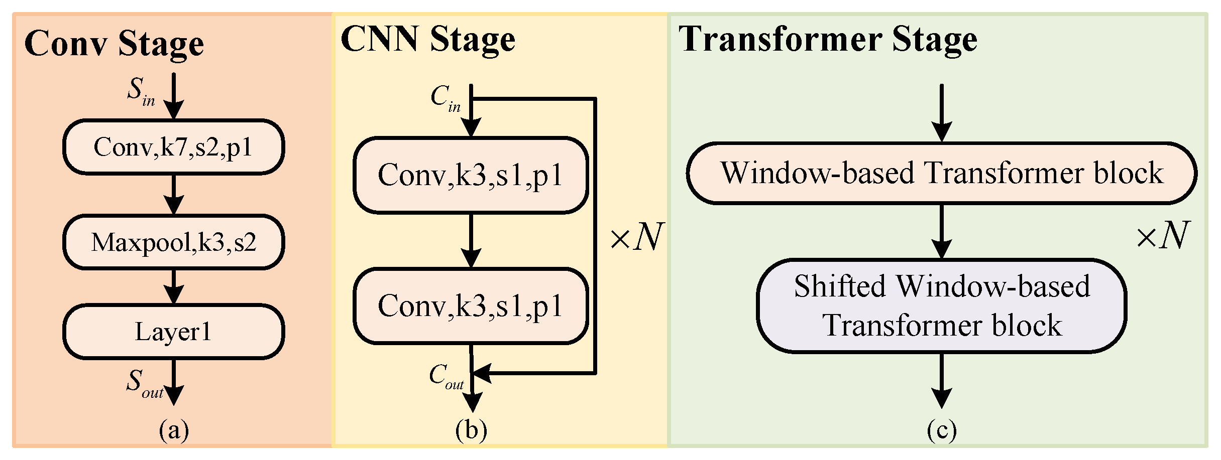
Conv, CNN, Transformer Stage architecture: (a) Conv Stage. (b) CNN Stage. (c) Transformer Stage.
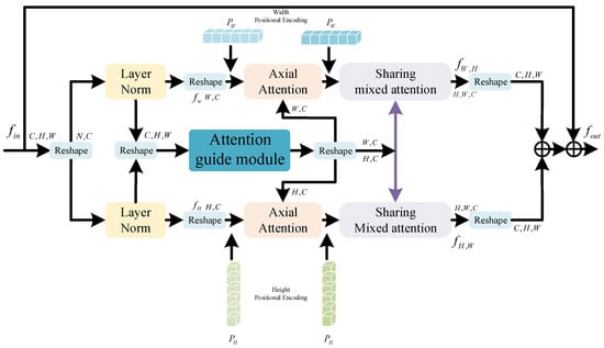
Figure 4.
Attention Guide Axial Sharing Mixed Attention module.

Table 1.
Architecture of the proposed method.
For a given remote sensing image with a size of X, a high-resolution image with certain semantic information is first generated through the Conv Stage, and the image size is . In order to obtain multi-scale features at the same feature level, a convolution is added before each layer after the Conv Stage, to increase the branch. Stage n increases the branch with a feature size of , and the channel is . Swin Transformer divides high-resolution features into non-overlapping patches. In contrast to image patches, there is no correlation between long sequence tokens. Pixels of the same type of objects in image patches have strong correlations, which can produce strong semantic associations. Therefore, unlike VIT [8] serializing images, in order to avoid excessive loss of semantic information in high-resolution features we use convolution to capture overlapping image patches from each feature. In the model, the patch size is 3 × 3, the overlap rate is 50%, and the stride is 1. Then, the data are flattened and projected into dimension . Finally, the Swin Transformer Stage based on the tandem Window-based Transformer block (W-T) and the Shifted Window-based Transformer block (SW-T) is used to establish long-distance dependencies between the data. In particular, this window-based encoder is susceptible to self-attention limitations. Therefore, by adding a parallel CNN sub-module to extract the pixel-level information of the feature, the semantic ambiguity problem caused by the limitation of the window is alleviated. The parallel Swin Transformer Stage and CNN Stage do not change the resolution and channel of the features.
In the feature fusion preparation stage, to facilitate information interaction among multi-scale features, the m features with varying resolutions obtained after the CT Stage undergo convolutional layers to enrich their semantic information. Subsequently, features are generated, comprising m groups of resolutions , each with m features, which are then passed on to the next stage. Low-resolution features will inevitably have semantic dilution after upsampling. We stitch features with the same resolution in the channel dimension. There are many irregular clouds, strip-shaped clouds, and small target clouds in the field of cloud and cloud shadow segmentation. Moreover, the number of global self-attention parameters are excessively large. Therefore, axial attention is first used to perform traditional self-attention in the H and W dimensions. However, although this self-attention can also achieve the effect of global modeling, it is limited by the size of the axial window, which limits the information exchange of some pixels in space. To this end, after this, SMA is used to build a bridge of information exchange in the H and W dimensions. In addition, in order to enhance attention to important information in V we incorporate original features that focus attention on channel and space. After AGASMA, the above operation is repeated, to obtain the final prediction mask.
3.2. Attention Guide Axial Sharing Mixed Attention Module (AGASMA)
Clouds and cloud shadows are irregular. Effectively segmenting thin clouds, strip clouds, and residual clouds has always been crucial for accurate cloud and cloud shadow segmentation [59]. This paper introduces a parallel multi-scale architecture to address these challenges, yet the issue of effectively integrating multi-scale information remains unresolved. To tackle this, we propose AGASMA in this paper. Figure 4 illustrates the architecture of the proposed model.
Unlike the traditional model based on axial attention, this paper used three branches to reconstruct the features. First, the input feature size was , and we serialized it and input it into three branches through the Layer normalization operation. Two of the branches mainly performed global attention on the features in the two dimensions of height and width. Because the Transformer ignores the position information when capturing the global information, the position encoding was embedded before the axial attention and SMA. For cloud detection tasks, there is usually a lot of noise in the dataset, which causes a lot of interference to accurate prediction. Therefore, this paper used an AGM based on channel and space to guide axial attention and V in SMA, so as to alleviate the interference of noise on prediction. Finally, the features were restored to the original size and fused with the original features.
3.2.1. Axial Attention
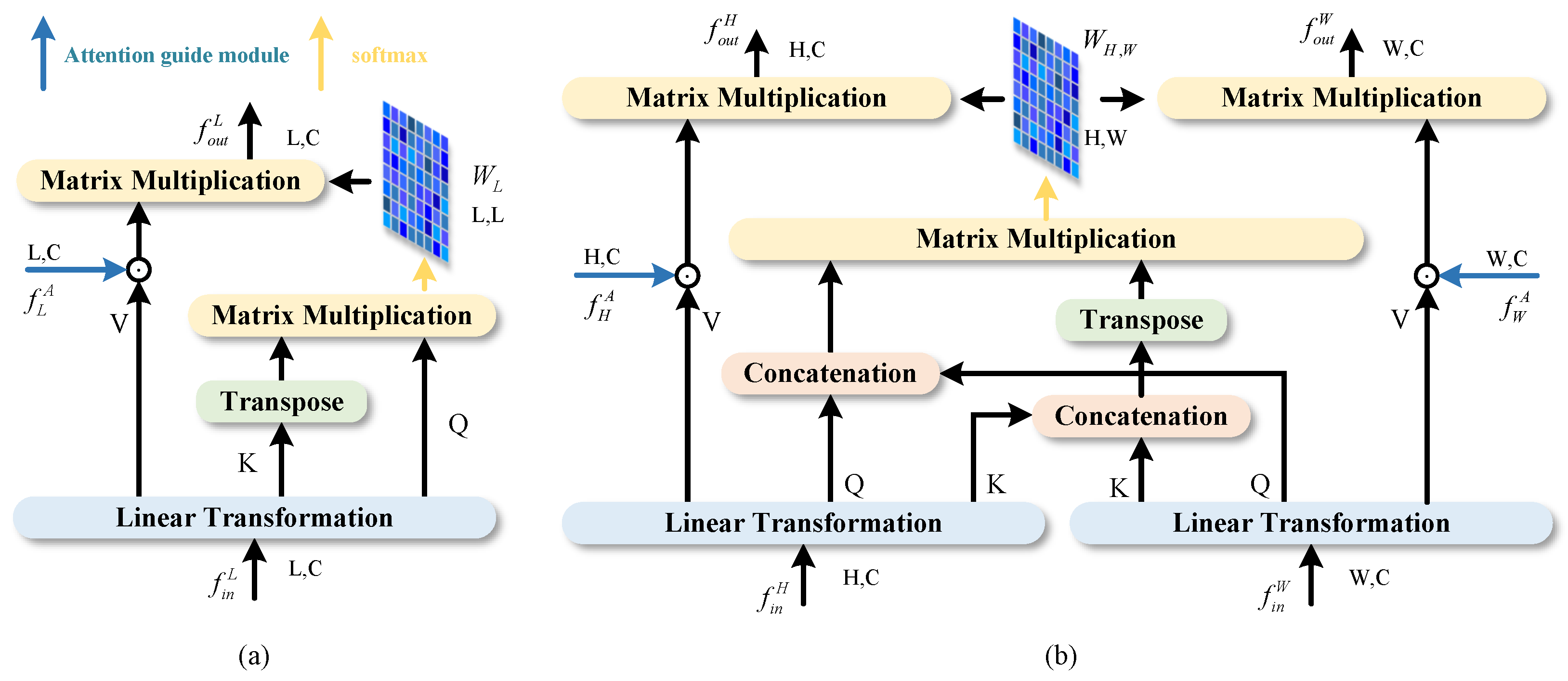
As mentioned above, although the traditional self-attention mechanism achieves the capability of global modeling, it consumes a lot of computing resources. To this end, this article introduces axial attention, as shown in Figure 5a. Axial attention can be represented as follows:
where represents Linear Transformation. The vector sequences , H, and W are, respectively, the height and weight of the features; C denotes the channel dimension; represents the feature from the AGM. Since axial attention only focuses on the information of height or width dimension, it alleviates the problem of excessive consumption of resources when using the self-attention mechanism, to a certain extent. At the same time, axial attention achieves better prediction results when dealing with images that contain strip features, such as strip clouds and residual clouds. However, limited by the size of the window, only using axial attention will lose the pixel dependencies between windows, which may lead to serious loss of semantic information. Axial information interaction between height and width seems to be a promising solution. For this reason, this paper adds SMA after axial attention.
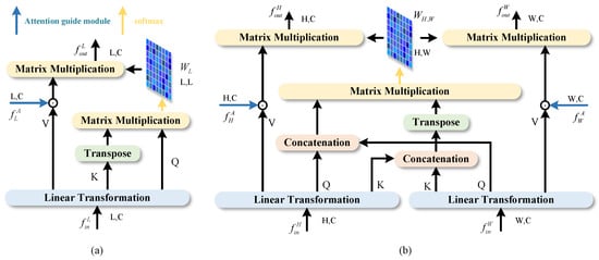
Figure 5.
Axial attention and SMA architecture diagram: (a) axial attention. (b) Sharing Mixed Attention.
3.2.2. Sharing Mixed Attention (SMA)
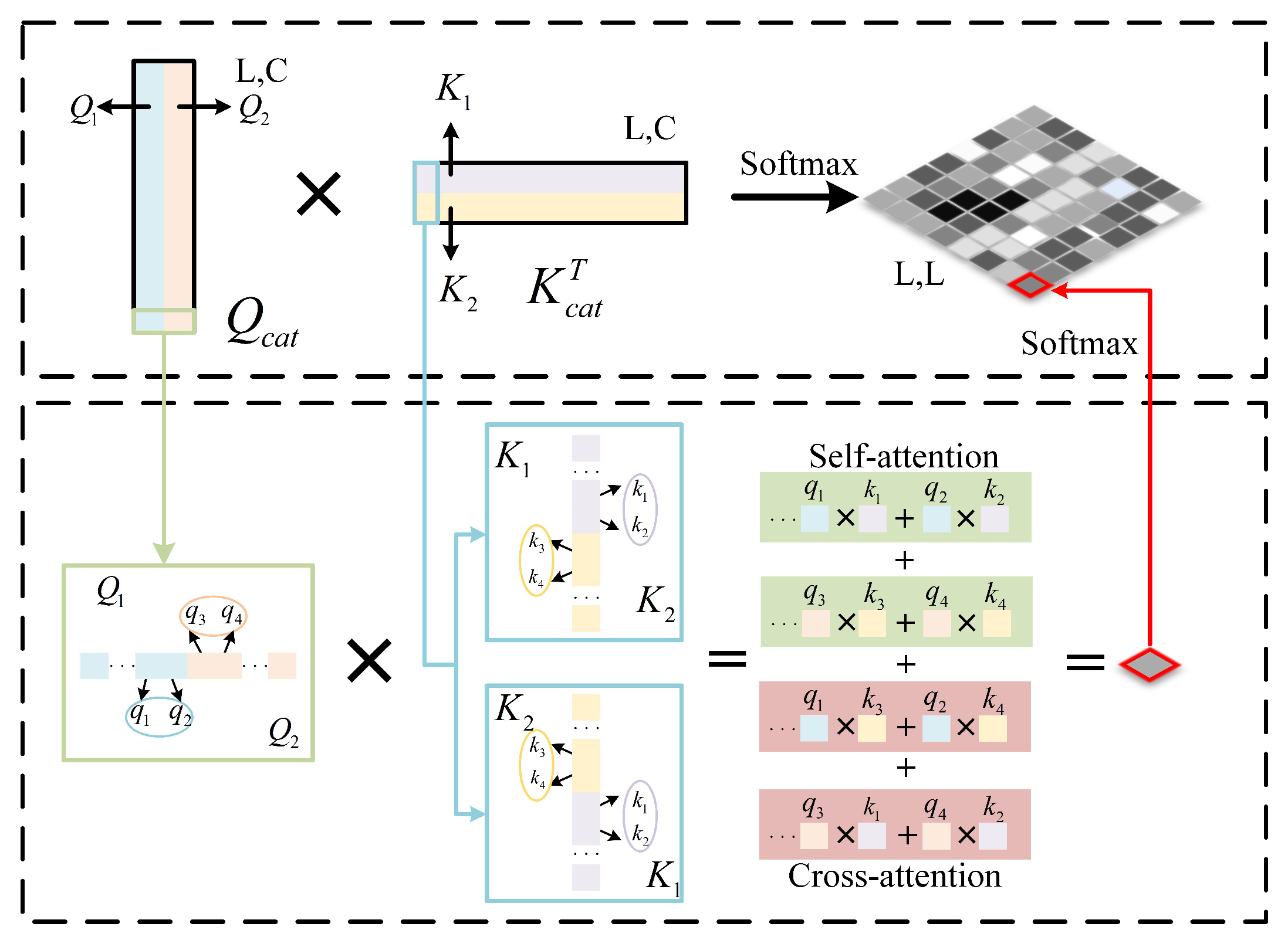
In order to fully integrate the information of different branches, this paper proposes SMA. As shown in Figure 5b, the shared information interaction method is used to exchange the axial information between height and width, and the original features after attention guidance are integrated into V. Firstly, the input features are processed from the axial attention, and the sizes are and , respectively. After Linear Transformation, , , and are obtained, respectively, and and are connected into and through a concatenation operation. In this way, the information between height and width is shared, and the number of heads of multi-head attention used in the module is 8. As shown in Figure 6, after sharing Q and K, self-attention and cross-attention can be learned at the same time, and Sharing Mixed Attention is obtained, which enhances the information exchange between different axes. Then, the similarity between global Q and K is obtained by Matrix Multiplication and Softmax processing. Like axial, the original features processed by the AGM are integrated into V, to enhance the effect of modeling in channel and spatial dimensions. ASMA can be expressed as follows:
where represents Concatenation, represents Sharing Mixed Attention, and indicates that the distribution involves both self-attention and cross-attention.
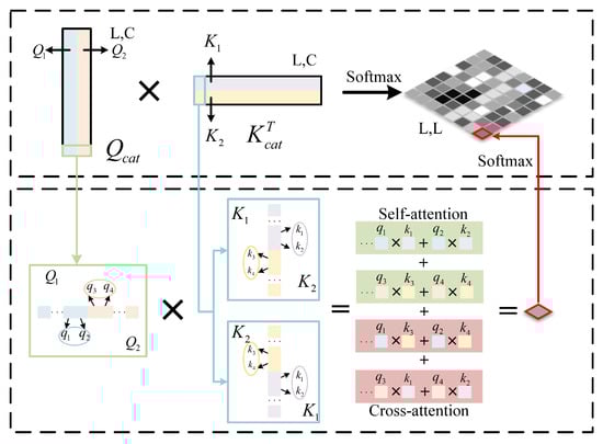
Figure 6.
Illustration of calculating Sharing Mixed Attention distribution.
In the actual segmentation of clouds and cloud shadows, there is much axial information, such as strip clouds and strip mountains. At this time, using axial attention can better extract axial feature information. When there is a need for global information to help accurate segmentation—for example, the background of the cloud in the picture is snow, and the background of the cloud shadow is the water area—the detection of the cloud and the cloud shadow is greatly affected by the background, and the global information perception ability is particularly important. At this time, the simple axial direction often cannot handle the information exchange of the entire picture well. While the self-attention mechanism effectively captures long-range dependencies, it typically demands substantial computational resources. Shared Q and K in SMA facilitate global information exchange, enhancing the model’s ability to capture global features while conserving computational resources.
Functionally, sharing the information of the two axes of height and width (mutual excitation of information from another scale) while retaining the information of their own attention effectively bridges the lack of global attention in a single axis. When conducting global attention, noise interference will inevitably occur. Adding the AGM, using Spatial Attention and Channel Attention guidance can effectively make up for the lack of anti-interference ability. In addition, the mutual guidance of the three branches reflects the advantages of both self-control and external control guidance. This can alleviate the lack of self-regulation, to a certain extent, and has the potential to suppress task-irrelevant interference, further promoting the learning effect of self-attention and enhancing more attention to the relevant objects.
3.2.3. Attention Guide Module (AGM)
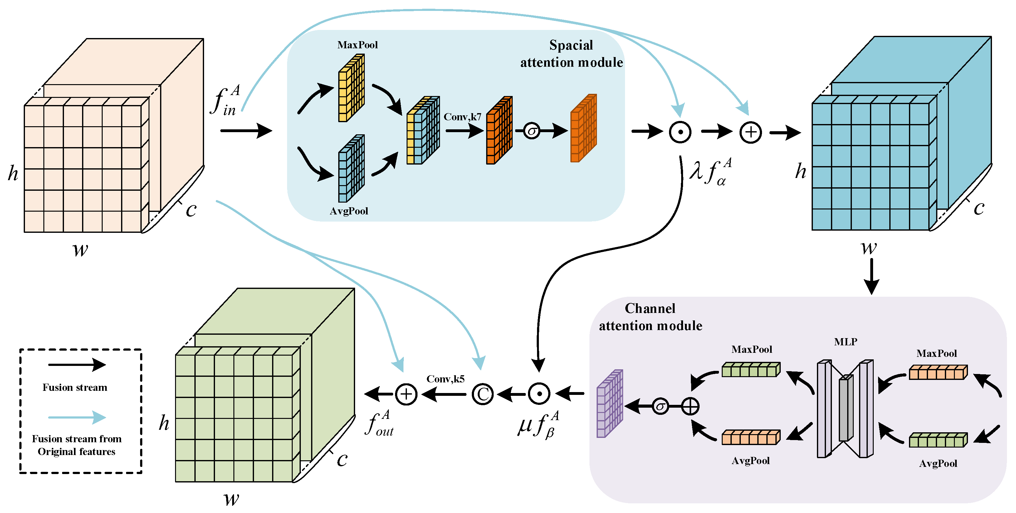
The texture distribution of cloud and cloud shadow is similar, and the target features, such as thin cloud and residual cloud, are not obvious. While models leveraging the self-attention mechanism provide a global perspective, they are susceptible to background noise interference. Recently, models integrating Channel Attention and Spatial Attention have demonstrated outstanding performance in reducing noise and prioritizing critical information [60]. Therefore, this paper constructed an AGM based on Channel Attention and Spacial Attention. The structure is shown in Figure 7, and we can express the AGM as follows:
where represents the sigmoid activation function, represents the global average pooling, represents spacial attention, and represents Channel Attention. The shared parameter and is initialized to 1 and then participates in back propagation for adaptive adjustment.

Figure 7.
Attention Guide Module.
In practical cloud detection tasks, there is often significant small target noise. To address this, we employ Channel Attention and Spatial Attention to highlight key information during cloud and cloud shadow detection. This enhances the detected features by reorganizing them across spatial and channel dimensions to better distinguish noise. Additionally, we incorporate a branch with original features, along with parameters and , to facilitate more effective weight redistribution.
The model based on self-attention is an attention mechanism for sequence data [16]. It calculates the correlation between different locations. At the same time, due to the need to reduce computing resources, the sequence length is limited by the size of the window, which weakens the global modeling ability of the Transformer, to some extent. Therefore, we add Spatial Attention, to strengthen the modeling of spatial dimension, better allocate the weight between pixels, and make Transformer more suitable for image tasks. At the same time, the above work lacks the modeling ability of the channel dimension. When clouds and shadows have similar distributions but different channels it may lead to confusion between objects [61]. Some methods (such as [12,56]) have shown that Channel Attention can enhance the ability of feature discrimination. Therefore, this paper introduces the CAM, to effectively model the channel. In addition, the SAM models the image space based on the pooling method, which can enhance the ability to obtain self-attention spatial information, to a certain extent. It can be seen from Figure 7 that the AGM contains two ways of information transmission. One is to strengthen the modeling of Spatial Attention and Channel Attention, and the other is to add the guidance of original features. This dual-branch guided architecture dynamically extracts crucial spatial and channel dimension information. It individually adjusts pixel weights across spatial channels, pixel by pixel, enhancing noise reduction and improving detection sensitivity for small-cloud edges and cloud shadow edges.
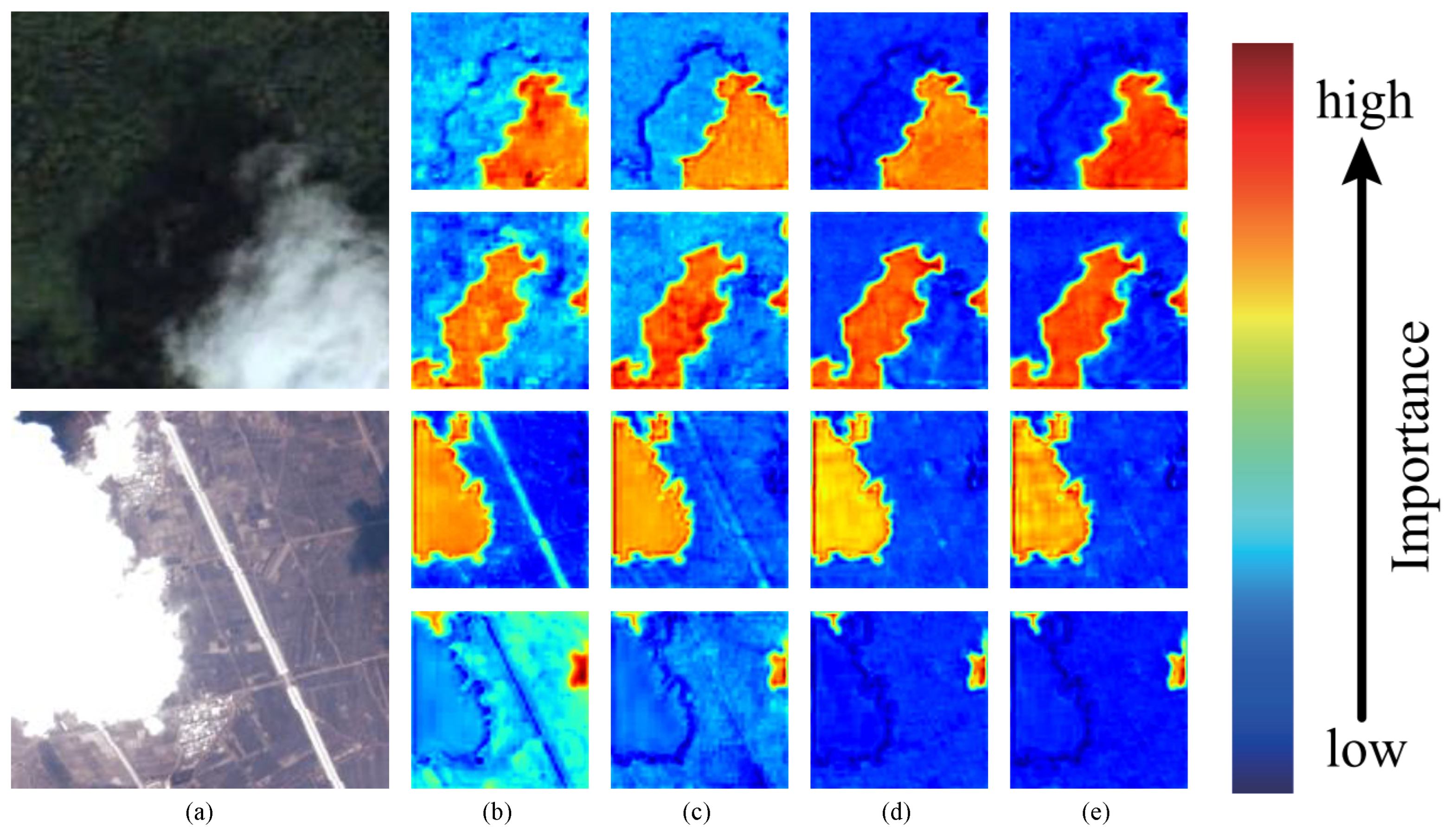
In Figure 8, a heatmap with different attention is visualized. The redder the image is, the higher the distribution weight is. The bluer the image is, the lower the weight is. The test image is shown in Figure 8a. The first line of each image is to detect the cloud, and the second line is to detect the cloud shadow; (b) and (c) are heatmaps without and with axial attention, respectively. It can be clearly seen that axial attention has excellent positioning ability for objects, and that boundary segmentation has also been improved. The position where attention needs to be focused becomes redder and the noise is reduced. After adding SMAtt, the information exchange between the two dimensions of height and width is strengthened. As shown in the heatmap (d), the model’s attention to the object that needs attention is significantly enhanced and the noise reduction effect is significant. At the same time, the segmentation boundary is clearer and the noise is further weakened. The Attention Guidance Module is added to (e) to further guide the axial attention in the spatial and channel dimensions. In addition to the predicted object, the attention is lighter, the pixel weight distribution is more reasonable, and the boundary prediction is at its clearest. The white road in the second image causes strong interference in the accurate detection of the cloud. After adding the axial attention, the interference is significantly reduced. After adding SMAtt, the interference of the white road is further reduced. After adding AGM, the interference is at its lowest and the attention to the cloud is also improved.
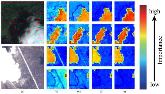
Figure 8.
Comparison of the effect of attention heatmap: (a) Test image. (b) Backbone. (c) Backbone + AxialAtt. (d) Backbone + AxialAtt + SMAtt. (e) Backbone + AxialAtt + SMAtt + AGM.
4. Datasets
4.1. Cloud and Cloud Shadow Dataset
The Cloud and Cloud Shadow dataset is our self-built dataset, consisting of manually calibrated data. The images in the dataset come from the high-resolution remote sensing image data on Google Earth, which are mainly collected by Landsat-8. Landsat-8 is equipped with an Operational Land Imager (OLI) and a thermal infrared sensor. There are 11 bands. We selected three of them—band 2 (Blue), band 3 (Green), and band 4 (Red)—with a spatial resolution of 30. The images in the dataset were mainly collected from the Yangtze River Delta, the Qinghai–Tibet Plateau, and from other regions, including complex backgrounds such as plateaus, cities, farmlands, waters, and hills. The original resolution was 4800 × 2692. In order to facilitate our research, we cut the original remote sensing image dataset to 224 × 224. After screening, we retained 22,000 images, of which 17,600 were training sets and 4400 were validation sets. The ratio of training set to validation set was 8:2. A sample is shown in Figure 9.
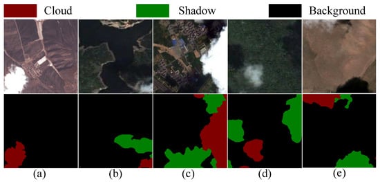
Figure 9.
Cloud and Cloud Shadow dataset part of the image display: (a) Hilly. (b) Waters. (c) Town. (d) Forest. (e) Desert.
4.2. SPARCS Dataset
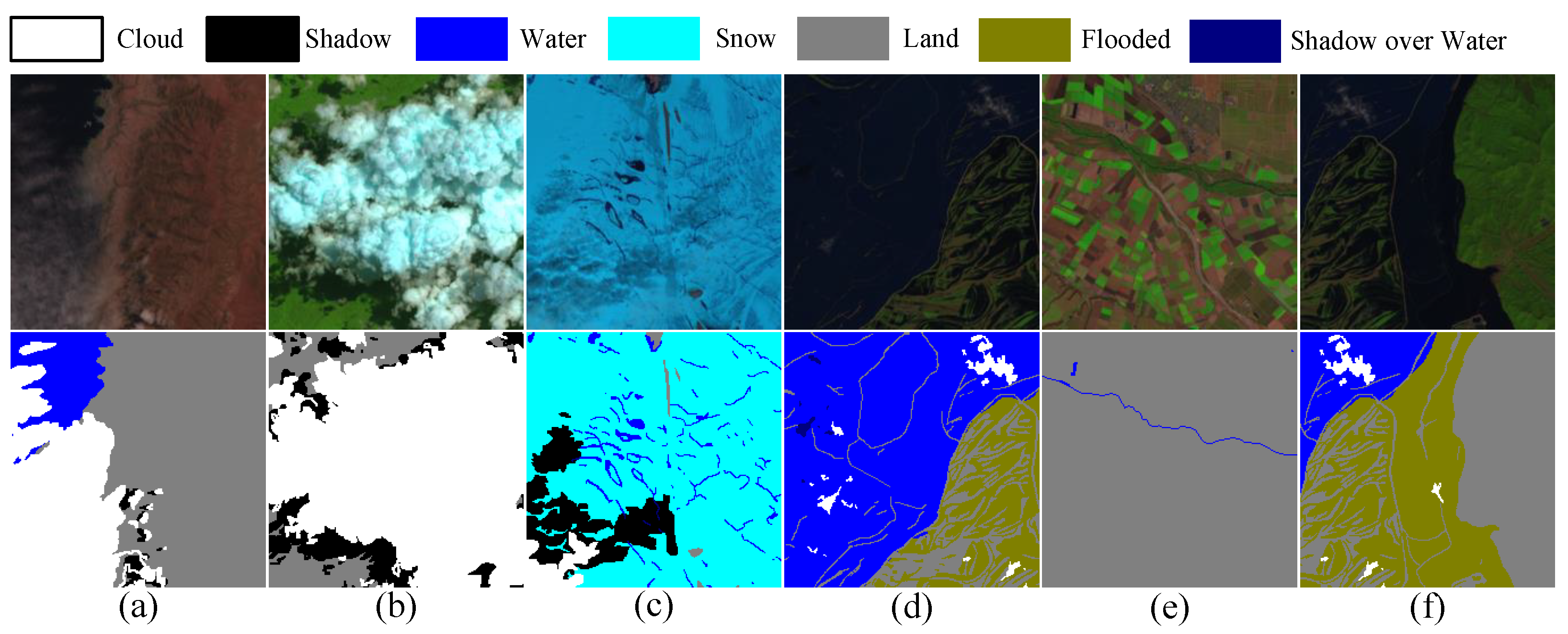
The SPARCS dataset is also derived from the Landsat8 satellite, created by M. Joseph Hughes [62]. The original dataset contains 80 images of 1000 × 1000, including various types of scenes, such as hilly, forest, snowfield, waters, farmland, flooded, etc. It is divided into seven categories: Cloud, Shadow, Water, Snow, Land, Flooded, and Shadow over Water. In order to facilitate our training, we cut the original image of 1000 × 1000 into a small image of 224 × 224 and obtained a total of 2880 images. In order to get more data for full experiments, we enhanced the data of the cropped images and we then divided the training set and the verification set according to a ratio of 8:2. The training set finally obtained 8000 images, and the verification set finally obtained 2000 images. The details of the dataset are shown in Figure 10 and Table 2.
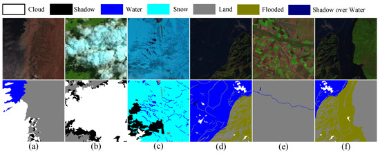
Figure 10.
SPARCS dataset part of the image display: (a) Hilly. (b) Forest. (c) Snowfield. (d) Waters. (e) Farmland. (f) Flooded.
Table 2.
SPARCS dataset.
4.3. CSWV Dataset
The CSWV dataset is a public dataset [63] that contains a large amount of information with cloud and snow content. The dataset contains many types of scenes, such as forest, town, desert, hilly, waters. There are three categories in the dataset: cloud, snow, and background. In order to facilitate our training, the original images in our dataset were cut into small images of 224 × 224 size, and a total of 4000 images were obtained. In order to obtain more data for full experiments, we enhanced the data of the cut images and then divided them into training and validation sets according to a ratio of 8:2. The training set finally obtained 8000 pictures and the verification set finally obtained 2000 pictures. The dataset sample is shown in Figure 11.
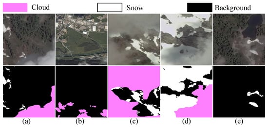
Figure 11.
CSWV dataset part of the image display: (a) Forest. (b) Town. (c) Desert. (d) Hilly. (e) Waters.
5. Experimental Analysis
The experiments in this paper were based on the PyTorch 1.12 platform, and the GPU used is NVIDIA 3070, produced by Taipei, China. In this paper, the Adam optimizer was used to optimize the experimental parameters, where was set to 0.9, was set to 0.999, and the learning rate strategy was the Step Learning Rate Schedule (StepLR). The formula is as follows:
where the benchmark learning rate is set to 0.001, the adjustment multiple is 0.95 times, the adjustment interval is 3, and the number of iterations is 300 times. The loss function used was the cross-entropy loss function, which is limited by the memory capacity of 8G. The experiment in this paper was carried out under a batchsize equal to 8.
We chose Pixel Accuracy (PA), Recall (R), category Mean Pixel Accuracy (MPA), F1, and Mean Intersection Over Union (MIOU) to evaluate the performance of different models in regard to cloud segmentation and cloud shadow segmentation. The formula of the above indicators is as follows:
Here, , , and denote the counts of pixels originally belonging to category i (j, i) but predicted as category i (i, j), respectively. TP represents the count of pixels correctly predicted for the categories (cloud, cloud shadow), while FN represents the count of pixels incorrectly predicted for the categories. K represents the total number of the categories, excluding the background.
5.1. Multi-Scale Fusion Experiment
In the traditional HRNet, multi-scale fusion is often used many times to exchange information with different scale features when adding new sub-modules. The multi-scale fusion method is depicted in the middle of the CT stage and AGASMA in Figure 2. Clearly, this model reduces the frequency of multi-scale fusions. This paper posits that frequent fusion of multi-scale information may hinder the extraction of deep semantic information. This conjecture is supported by the results in Table 3, which display the MIOU (%) from the experiments on the specified dataset.
Table 3.
Multi-scale fusion experiment.
In the table, ‘CC’ represents the Cloud and Cloud Shadow dataset. ’SPARCS’ represents the SPARCS dataset. ‘CSWV’ represents the CSWV dataset. ‘Ours (HRNet)’ represents that our model used the same number of multi-scale fusions as HRNet; that is, a multi-scale fusion layer was added between every four layers in L2 and L3, as shown in Table 2. ‘Ours’ represents our model. As observed from the table, reducing the number of multi-scale fusions improved the MIOU (%) in our experiments across the three datasets.
5.2. Backbone Fusion Experiment
In this paper, when extracting features, the architecture of maintaining high-resolution features throughout the process was adopted. When extracting features using sub-modules, the parallel scheme of the Transformer and CNN sub-modules was selected. By constructing a parallel interaction platform between the Transformer and the CNN (the fusion of fine features and rough features) different scale features were realized. To explore the optimal combination, experiments were conducted, and the results are shown in Table 4.
Table 4.
Backbone fusion experiment.
In the experiment, we selected eight ways of combining the CNN and the Transformer on the Cloud and Cloud Shadow dataset for research, with the MIOU (%) as the final evaluation basis. From the table, it is evident that the combination of Swin and Basic Block achieved the highest MIOU value in the experiment, having achieved 92.68%. Therefore, this scheme was selected as the Backbone of this paper.
5.3. Comparative Study of Attention Mechanism
As mentioned above, this paper uses a full-range high-resolution network. Hence, repeating the fusion of multi-scale information becomes necessary to fully integrate and effectively extract information. This paper proposes axial attention, which models the features globally in height and width, respectively, greatly enriching the semantic information of the features. However, the axial attention window is limited, making SMA a promising solution in this paper. A comparative study of SMA is presented in Table 5. The result in the table represents the MIOU (%) from the experiment on the specified dataset.
Table 5.
Comparative study of attention mechanisms.
In the table, ‘Without’ represents the case without Sharing-mixed-attention. ‘Cross-attention’ represents in Equation (12), which uses only cross-attention. ‘Mixed-attention (a)’ represents in Equation (12). ‘Mixed-attention (b)’ represents in Equation (12). In the two mixed-attention schemes, both self-attention and cross-attention are utilized. The ‘Sharing-mixed-attention’ scheme in this paper integrated identical self-attention and cross-attention into both branches. As shown in Table 5, it was verified that the MIOU (%) of the attention in the three datasets was improved, and that the MIOU (%) on different datasets was improved by 1.36%, 2.05%, and 1.27%, respectively, which fully reflects the effectiveness of Sharing-mixed-attention in dealing with multi-scale information fusion.
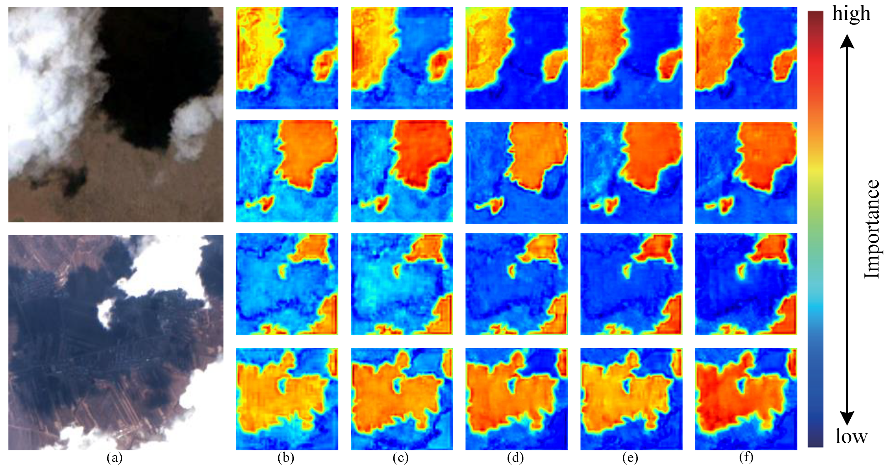
Traditional axial attention can only model the features globally in a single dimension, and it is easy to lose the dependence of pixels between some dimensions. In contrast, in our model design, Sharing-mixed-attention can effectively alleviate the information-loss problem of single-dimensional modeling, and it is used to better model the feature interaction between multi-scale images through shared part representation. A comparative study of a set of attention mechanisms is visualized in Figure 12. From the figure, it is evident that the attention mechanism proposed in this paper effectively identifies clouds and cloud shadows in scenes with noise and thin clouds by assigning higher weights accordingly. Furthermore, compared to other attention fusion methods, our model exhibits superior performance in reducing interference.
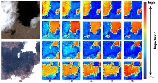
Figure 12.
Comparative study of attention mechanisms: (a) Test image. (b) Without. (c) Cross-attention. (d) Mixed-attention (a). (e) Mixed-attention (b). (f) Sharing-mixed-attention.
5.4. Network Ablation Experiments
To evaluate the performance of the proposed network structure and modules, we applied our Backbone (that is, the number of HRNet multi-scale fusions was the same as the architecture in this paper) to perform ablation studies on the Cloud and Cloud Shadow dataset, the SPARCS dataset, and the CSWV dataset. All the parameters in the experiment were set to default values, and our experimental results are presented in Table 6. The performance of our model was primarily evaluated using the MIOU parameter.
Table 6.
Network ablation experiments.
- Effect of CNN and Transformer cross-architecture: The results are presented in Table 6. The architecture incorporating CNN and Transformer parallel sub-modules effectively enhanced the segmentation performance of the Backbone. By substituting certain CNN sub-modules with Transformer sub-modules, we achieved a fusion of fine and coarse features at the same feature level. Compared with Backbone, this model improved the MIOU by 0.61%, 1.48%, and 0.40% on the three datasets, respectively. In Figure 13, the heatmaps before and after the Swin Transformer module are visualized. From the figure, it is evident that the global receptive field enhanced the model’s semantic information and improved target prediction accuracy.
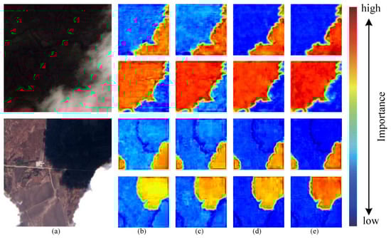 Figure 13. Network ablation experiment: (a) Test image. (b) Backbone. (c) Backbone + Swin. (d) Backbone + Swin + ASMA. (e) Backbone + Swin + AGASMA.
 - Effect of Axial Sharing Mixed Attention (ASMA) module: Table 6 shows that after adding the Axial Sharing Mixed Attention (ASMA) module, the segmentation results increased by 1.11%, 1.55%, and 1.28% on the MIOU. It is verified that this attention mechanism for multi-scale fusion can effectively reconstruct the dependencies between pixels. More intuitively, the visual segmentation results are shown in Figure 13. For the above image, the use of ASMA alleviated the interference of the thin cloud and residual cloud on the boundary segmentation. For the second image, high ground noise significantly affected the accurate identification of clouds and cloud shadows, but using ASMA greatly reduced this interference. These results demonstrate that integrating ASMA to efficiently fuse multi-scale features enhances the model’s segmentation accuracy in complex backgrounds, including thin clouds, residual clouds, and high noise.
- Effect of the Attention Guide Module: As shown in Table 6, we added the CBAM and the AGM on the basis of Backbone + Swin + ASMA, respectively. Our experiments showed that AGM is significantly better than CBAM in performance, and that the MIOU was improved by 0.29%, 0.55%, and 0.24% on the three datasets, respectively, verifying the effectiveness of the AGM in our network. For the noise-interference and target-positioning problems mentioned above, our model achieved the best results. In Figure 13, the visualization indicates that the areas of cloud and cloud shadow positioning appear more red, highlighting a concentrated weight distribution in the target areas. Noise interference was minimized, resulting in less impact on non-target areas, which appear bluer. The results demonstrate that integrating the ASM guided attention mechanism for feature fusion effectively reduces noise interference and enhances the model’s accuracy in target positioning.
5.5. Comparative Experiments of Different Algorithms on Cloud and Cloud Shadow Dataset
To fully assess our model’s performance, we conducted comparative experiments on the Cloud and Cloud Shadow dataset. The experiments compared the current cutting-edge semantic segmentation techniques. To ensure experiment objectivity, we used default parameters. In this experiment, Flops and Parameter were calculated on an image with a size of 224 × 224 × 3. The detailed data of this experiment are recorded in Table 7.
Table 7.
Comparative experiments of different algorithms in the Cloud and Cloud Shadow dataset.
In our experiment, we compared some existing popular models. When selecting the comparison model, we took into account the similarity between other models and our model. Among these, UNet [4], SwinUNet [47], DBNet [33], and DBPNet [52] use encoder and decoder structures based on UNet, to be compared with the model in this paper. CVT [34], SwinUNet, PVTv2 [65] were compared with the model in this paper, as encoders based on the Transformer. DANet [56] and CCNet [17] use attention to reconstruct the dependencies between pixels, which is similar to the model in this paper. CloudNet [27] and DBNet, as cloud detection networks, were compared with the model in this paper. CMT [64], MPvit [13], HRvit [66], DBNet, DBPNet employ a method that combines the CNN and the Transformer, as did this article. DeepLabv3 [5], MPvit, and PSPNet [37] adopt multi-scale to strengthen semantic information, which is similar to this paper. HRNet, HRvit, and OCRNet [67] are similar to this article’s architecture.
Table 7 presents the results of each semantic segmentation method. Our model was superior to other methods, except that P (%) and R (%) in Cloud were slightly lower than OCRNet and HRvit. UNet et al. used the encoding-and-decoding method based on UNet as the baseline, which can effectively alleviate the serious problem of information loss in high-resolution prediction maps. Our model maintained a high-resolution representation throughout the process, ensuring richer semantic information in the features. PVTv2 and others used global receptive fields to obtain information. Although it used a similar architecture to the CNN encoder, which was conducive to dense prediction and had the highest MIOU in the Transformer model, our model was 1.83% higher than the MIOU. The dual attention mechanism of models such as DANet was slightly inferior to our ASMA in global modeling. DeepLabv3 and others added multi-scale modules to further enrich the semantic information of the high semantic features. Although OCRNet and others were similar to the architecture of our model, there was still a big gap between the MIOU value and our model. Most of the other models combining CNN and Transformer achieved good results for the MIOU. Most of them adopted the same parallel structure as this paper, thus verifying, to some extent, that combining fine and coarse features can effectively improve model prediction accuracy.
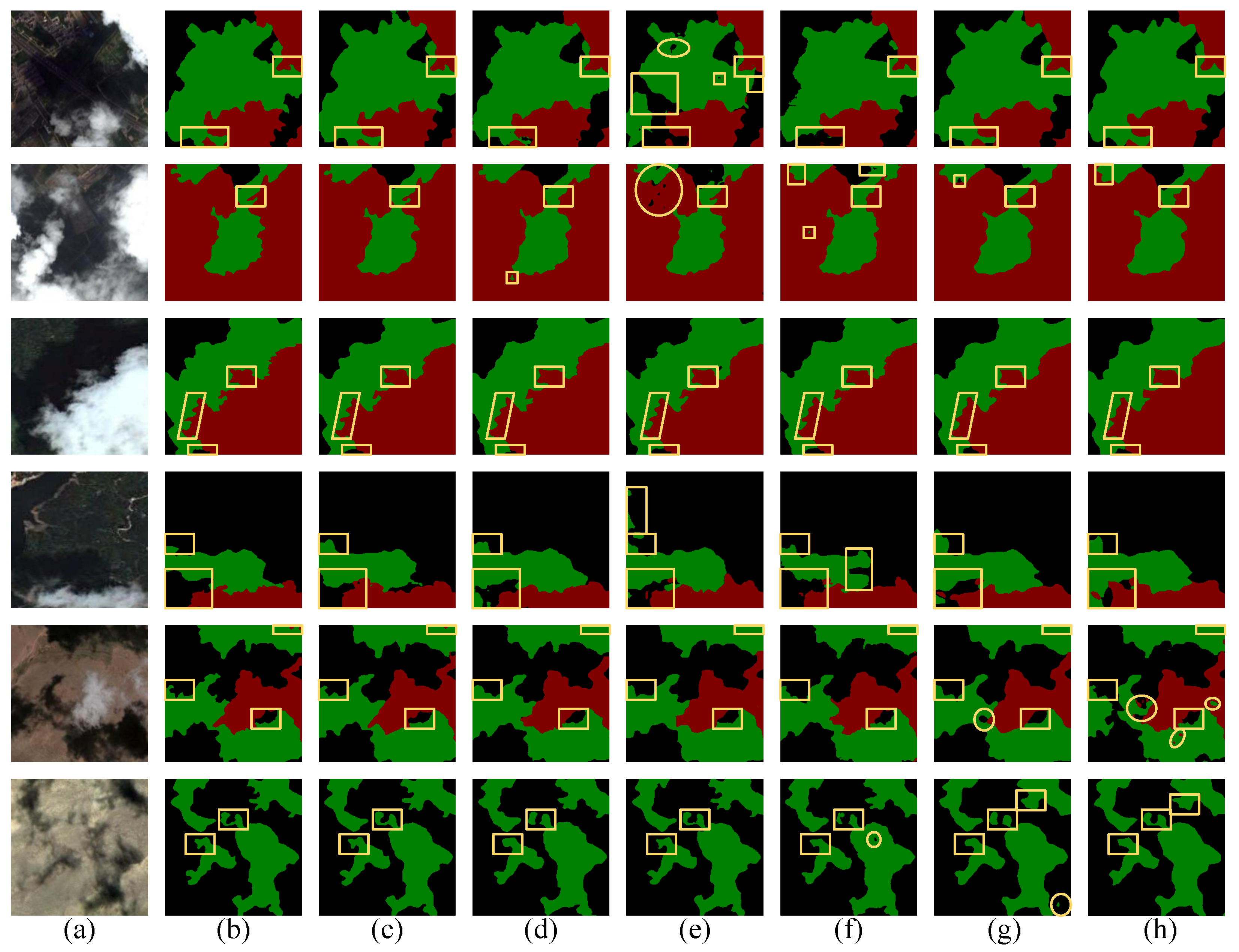
Figure 14 and Figure 15 display the prediction results of several models, showcasing their superior performance, as summarized in Table 7. It is evident that while the PSPNet, a CNN-based model, leveraged the PPM to compensate for global modeling deficiencies, there was still a big gap in the global modeling of the Transformer. In the prediction map, the edge segmentation was not obvious, and the edge thin cloud detection was difficult. DBNet, like our model, is a cloud detection model that combines the CNN and the Transformer. As shown in Figure 14, DBNet missed thin clouds and some cloud shadows in the first image, and there was a big gap with our model in the boundary segmentation of the second, third, fourth, and fifth images. In the last image, thin cloud shadows were missed. DBNet also had a high false detection rate in Figure 15. This was due to its simple splicing when dealing with the fusion problem of the CNN and the Transformer, and the unreasonable distribution of feature weights, resulting in a large amount of information redundancy. Compared to the other models, our predictions improved the accuracy of cloud and cloud shadow edge segmentation.
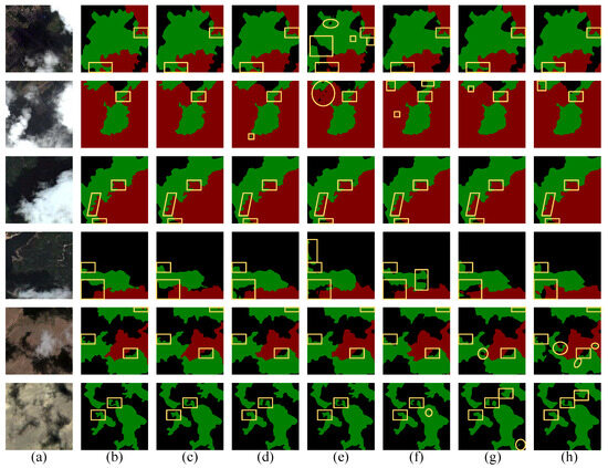
Figure 14.
Comparison of different methods in different scenarios for the Cloud and Cloud Shadow dataset: (a) Test images. (b) Label. (c) Ours. (d) DBPNet. (e) OCRNet. (f) DBNet. (g) HRvit. (h) PSPNet.
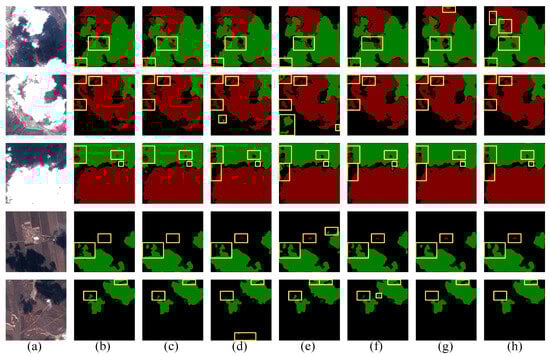
Figure 15.
Anti-noise comparison of different models in the Cloud and Cloud Shadow dataset: (a) Test images. (b) Label. (c) Ours. (d) DBPNet. (e) OCRNet. (f) DBNet. (g) HRvit. (h) PSPNet.
As shown in Figure 14, in the first three lines, there was a large gap between our model and other models, in terms of edge recognition of thin clouds and cloud shadows. In line 4, other methods incorrectly identified the water area as a cloud shadow, while our model made an accurate judgment. In the last two lines, our model also showed excellent positioning ability for residual clouds and irregular clouds. In addition, Figure 15 displays prediction maps demonstrating the model’s resistance to interference. Specifically, our model exhibited fewer false detections in areas with high-brightness houses and roads. In contrast, other models performed poorly in the face of such strong interference. On the whole, the model presented in this paper achieved excellent performance in resisting interference.
5.6. Comparative Experiments of Different Algorithms in SPARCS Dataset
Table 8 presents the segmentation results of each method on the SPARCS Dataset, validating the effectiveness of our model (with experimental parameters consistent with the Cloud and Cloud Shadow dataset). Our model achieved superior performance, with the MIOU at 81.48% and F1 at 85.52%, surpassing the other models. In terms of single-precision metrics, our model achieved the highest values on Cloud, Shadow, Snow, and Land, slightly lower than DeepLabv3 on Water and Shadow over Water, and slightly lower than DBPNet on Flooded. On the multi-class dataset, the global view becomes particularly important. DeepLabv3, which benefits from the receptive field expander ASPP, showed strong performance on this dataset. However, some CNN-based models, such as UNet and DANet, did not perform well. Although our model is based on the CNN and Transformer parallel structure, ASMA provides a global view and effectively improves the ability to obtain spatial information. Therefore, our model achieved excellent results in multi-classification networks.
Table 8.
Comparative experiments of different algorithms on SPARCS dataset.
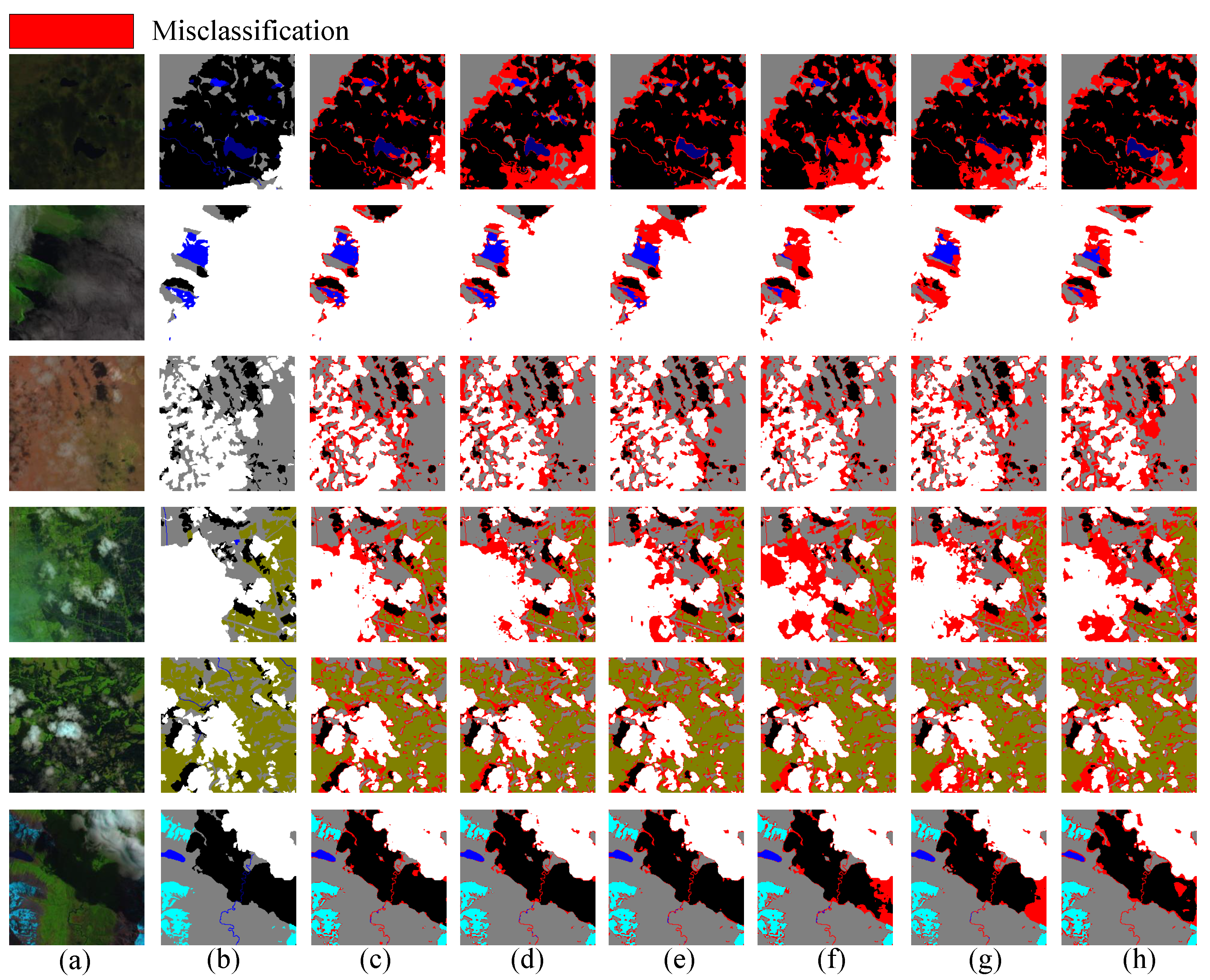
In Figure 16, we visualize the segmentation results on the SPARCS dataset. The red areas indicate missed and false detections. In the first row, the dim light made it harder to identify thin clouds, water, and cloud shadows, leading to more severe false and missed detections by the model. In contrast, the prediction effect of our model was better. In the second line, it was very difficult to accurately identify the waters covered by thin clouds. Here, the advantages of mixing the spatial features and local features of our model were revealed. In the third row, the cloud appeared lighter in color, and there were more small targets. The architecture of our high-resolution representation ensured our excellent performance. In the fourth and fifth lines, the lines of flood were more complex. Compared with the other models, our model more accurately distinguished flood and land. In the last line, the cloud shadow color was darker, and it was easy to misdetect into waters. OCRNet and DBNet had a large range of misdetection.
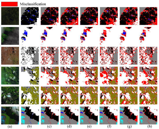
Figure 16.
Comparison of different methods in different scenarios of SPARCS dataset: (a) Test images. (b) Label. (c) Ours. (d) DBPNet. (e) DeepLabv3. (f) OCRNet. (g) DBNet. (h) MPvit.
5.7. Comparative Experiments of Different Algorithms in CSWV Datasets
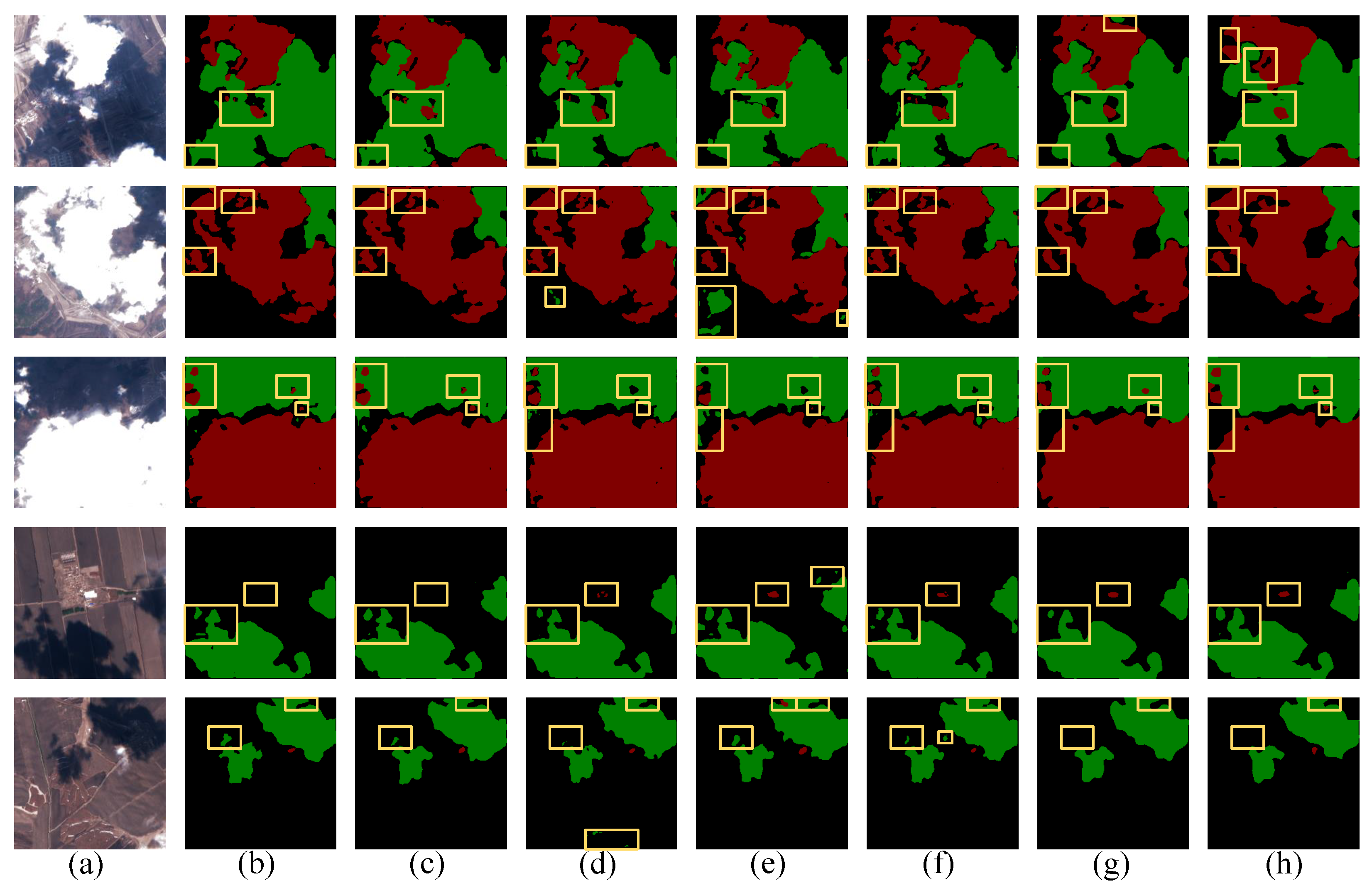
To further verify our model’s generalization ability, Table 9 shows the segmentation performance of each method on the CSWV dataset (the experimental parameters were consistent with the Cloud and Cloud Shadow dataset). Our model achieved the highest scores in PA (%), MPA (%), R (%), F1 (%), and MIOU (%). In CSWV, the similar colors and shapes of clouds and snow, along with complex backgrounds like thin clouds and snow cover, increased detection difficulty. Additionally, light intensity significantly affected the model’s performance, posing a challenge in accurately segmenting the target.
Table 9.
Comparative experiments of different algorithms in CSWV dataset.
A set of segmentation results on the CSWV dataset is visualized in Figure 17. As shown in the top row, the boundary of the thin cloud was not well-recognized, HRNet lacked the global receptive field, and DBNet, DeepLabv3, and DBPNet had weak spatial information acquisition capabilities, resulting in a large range of false detection. As shown in the second line, our model better dealt with the problem of cloud blocking snow. DeepLabv3 misdetected snow as clouds, and other models failed to deal with the problem of cloud–snow boundary segmentation. As shown in the third row, the cloud was too thin to be distinguished by the naked eye. Our model had the fewest missed detections and false positives. As shown in the fourth row, the distribution of snow was finer and the target area was smaller. OCRNet and DBPNet failed to identify snow, and our model recognition effect was good. As shown in the fifth row, the distribution of cloud and snow was more complex, resulting in more severe false detections and missed detections. In dealing with the boundary between cloud and cloud shadow, our model performed well. As shown in the sixth row, there was a problem of thin clouds blocking snow. DBPNet, DeepLabv3, DBNet, and HRNet all exhibited many false detections. In contrast, our model showed better accuracy with fewer false detections.
Figure 17.
Comparison of different methods in different scenarios for CSWV dataset: (a) Test images. (b) Label. (c) Ours. (d) OCRNet. (e) DBPNet. (f) DeepLabv3. (g) DBNet. (h) HRNet.
6. Conclusions
This paper focused on enhancing the accurate recognition of cloud and cloud shadow by extracting more comprehensive semantic and spatial information from images. We used parallel CNN and Transformer sub-modules on Backbone to construct a semantic segmentation architecture that maintains high-resolution representation throughout. Specifically, the proposed CNN and Transformer parallel structure effectively aggregates spatial and local information. In addition, for the problem of multi-resolution aggregation, ASMA was engineered to address the issue of information loss during the fusion of multi-resolution networks, the interaction between height and width information, and the reconstruction of the dependencies between pixels. At the same time, the global modeling capability partially mitigates the issue of limited window size in Swin Transformer models. However, when dealing with the problem of object segmentation, we should not only consider the modeling of spatial dimension. Therefore, we propose the AGM, which reduces the limitation of the self-attention mechanism, to a certain extent. Our experimental results demonstrated the effectiveness of our model on various datasets, including the Cloud and Cloud Shadow dataset, the SPARCS dataset, and the CSWV dataset.
Author Contributions
Conceptualization, G.G. and Z.W.; methodology, L.W.; software, G.G.; validation, L.W. and H.L.; formal analysis, Z.W.; investigation, Z.Z.; resources, L.W.; data curation, L.Z. and G.G.; writing—original draft preparation, G.G.; writing—review and editing, Z.W. and Z.Z.; visualization, L.Z. and G.G.; supervision, L.W.; project administration, L.W.; funding acquisition, L.W. All authors have read and agreed to the published version of the manuscript.
Funding
This work was supported in part by the National Natural Science Foundation of PR China (42075130).
Data Availability Statement
Data are contained within the article.
Conflicts of Interest
The authors declare no conflicts of interest.
References
- Ceppi, P.; Nowack, P. Observational evidence that cloud feedback amplifies global warming. Proc. Natl. Acad. Sci. USA 2021, 118, e2026290118. [Google Scholar] [CrossRef]
- Chen, K.; Dai, X.; Xia, M.; Weng, L.; Hu, K.; Lin, H. MSFANet: Multi-Scale Strip Feature Attention Network for Cloud and Cloud Shadow Segmentation. Remote Sens. 2023, 15, 4853. [Google Scholar] [CrossRef]
- Carn, S.A.; Krueger, A.J.; Krotkov, N.A.; Yang, K.; Evans, K. Tracking volcanic sulfur dioxide clouds for aviation hazard mitigation. Nat. Hazards 2009, 51, 325–343. [Google Scholar] [CrossRef]
- Ronneberger, O.; Fischer, P.; Brox, T. U-net: Convolutional networks for biomedical image segmentation. In Proceedings of the Medical Image Computing and Computer-Assisted Intervention–MICCAI 2015: 18th International Conference, Munich, Germany, 5–9 October 2015; Proceedings, Part III 18. Springer: Berlin/Heidelberg, Germany, 2015; pp. 234–241. [Google Scholar]
- Chen, L.C.; Zhu, Y.; Papandreou, G.; Schroff, F.; Adam, H. Encoder-decoder with atrous separable convolution for semantic image segmentation. In Proceedings of the European Conference on Computer Vision (ECCV), Munich, Germany, 8–14 September 2018; pp. 801–818. [Google Scholar]
- Chen, K.; Xia, M.; Lin, H.; Qian, M. Multi-scale Attention Feature Aggregation Network for Cloud and Cloud Shadow Segmentation. IEEE Trans. Geosci. Remote Sens. 2023, 61, 5612216. [Google Scholar]
- Sun, K.; Xiao, B.; Liu, D.; Wang, J. Deep high-resolution representation learning for human pose estimation. In Proceedings of the IEEE/CVF Conference on Computer Vision and Pattern Recognition, Long Beach, CA, USA, 15–20 June 2019; pp. 5693–5703. [Google Scholar]
- Dosovitskiy, A.; Beyer, L.; Kolesnikov, A.; Weissenborn, D.; Zhai, X.; Unterthiner, T.; Dehghani, M.; Minderer, M.; Heigold, G.; Gelly, S.; et al. An image is worth 16 × 16 words: Transformers for image recognition at scale. arXiv 2020, arXiv:2010.11929. [Google Scholar]
- Ren, H.; Xia, M.; Weng, L.; Hu, K.; Lin, H. Dual-Attention-Guided Multiscale Feature Aggregation Network for Remote Sensing Image Change Detection. IEEE J. Sel. Top. Appl. Earth Obs. Remote Sens. 2024, 17, 4899–4916. [Google Scholar] [CrossRef]
- Dai, X.; Xia, M.; Weng, L.; Hu, K.; Lin, H.; Qian, M. Multi-Scale Location Attention Network for Building and Water Segmentation of Remote Sensing Image. IEEE Trans. Geosci. Remote Sens. 2023, 61, 5609519. [Google Scholar] [CrossRef]
- Ren, W.; Wang, Z.; Xia, M.; Lin, H. MFINet: Multi-Scale Feature Interaction Network for Change Detection of High-Resolution Remote Sensing Images. Remote Sens. 2024, 16, 1269. [Google Scholar] [CrossRef]
- Yin, H.; Weng, L.; Li, Y.; Xia, M.; Hu, K.; Lin, H.; Qian, M. Attention-guided siamese networks for change detection in high resolution remote sensing images. Int. J. Appl. Earth Obs. Geoinf. 2023, 117, 103206. [Google Scholar] [CrossRef]
- Lee, Y.; Kim, J.; Willette, J.; Hwang, S.J. Mpvit: Multi-path vision transformer for dense prediction. In Proceedings of the IEEE/CVF Conference on Computer Vision and Pattern Recognition, New Orleans, LA, USA, 18–24 June 2022; pp. 7287–7296. [Google Scholar]
- Xu, J.; Xiong, Z.; Bhattacharyya, S.P. PIDNet: A Real-Time Semantic Segmentation Network Inspired by PID Controllers. In Proceedings of the IEEE/CVF Conference on Computer Vision and Pattern Recognition, Vancouver, BC, Canada, 17–24 June 2023; pp. 19529–19539. [Google Scholar]
- Dai, X.; Chen, K.; Xia, M.; Weng, L.; Lin, H. LPMSNet: Location pooling multi-scale network for cloud and cloud shadow segmentation. Remote Sens. 2023, 15, 4005. [Google Scholar] [CrossRef]
- Vaswani, A.; Shazeer, N.; Parmar, N.; Uszkoreit, J.; Jones, L.; Gomez, A.N.; Kaiser, Ł.; Polosukhin, I. Attention is all you need. Adv. Neural Inf. Process. Syst. 2017, 30. [Google Scholar]
- Huang, Z.; Wang, X.; Huang, L.; Huang, C.; Wei, Y.; Liu, W. Ccnet: Criss-cross attention for semantic segmentation. In Proceedings of the IEEE/CVF International Conference on Computer Vision, Seoul, Republic of Korea, 27 October–2 November 2019; pp. 603–612. [Google Scholar]
- Feng, Y.; Jiang, J.; Xu, H.; Zheng, J. Change detection on remote sensing images using dual-branch multilevel intertemporal network. IEEE Trans. Geosci. Remote Sens. 2023, 61, 4401015. [Google Scholar] [CrossRef]
- Chen, C.F.R.; Fan, Q.; Panda, R. Crossvit: Cross-attention multi-scale vision transformer for image classification. In Proceedings of the IEEE/CVF International Conference on Computer Vision, Montreal, BC, Canada, 11–17 October 2021; pp. 357–366. [Google Scholar]
- Manolakis, D.G.; Shaw, G.A.; Keshava, N. Comparative analysis of hyperspectral adaptive matched filter detectors. In Proceedings of the Algorithms for Multispectral, Hyperspectral, and Ultraspectral Imagery VI, Orlando, FL, USA, 23 August 2000; SPIE: Bellingham, WA, USA, 2000; Volume 4049, pp. 2–17. [Google Scholar]
- Liu, X.; Xu, J.m.; Du, B. A bi-channel dynamic thershold algorithm used in automatically identifying clouds on gms-5 imagery. J. Appl. Meteorl. Sci. 2005, 16, 134–444. [Google Scholar]
- Ma, F.; Zhang, Q.; Guo, N.; Zhang, J. The study of cloud detection with multi-channel data of satellite. Chin. J. Atmos. Sci.-Chin. Ed. 2007, 31, 119. [Google Scholar]
- Ji, H.; Xia, M.; Zhang, D.; Lin, H. Multi-Supervised Feature Fusion Attention Network for Clouds and Shadows Detection. ISPRS Int. J. Geo-Inf. 2023, 12, 247. [Google Scholar] [CrossRef]
- Ding, L.; Xia, M.; Lin, H.; Hu, K. Multi-Level Attention Interactive Network for Cloud and Snow Detection Segmentation. Remote Sens. 2024, 16, 112. [Google Scholar] [CrossRef]
- Gkioxari, G.; Toshev, A.; Jaitly, N. Chained predictions using convolutional neural networks. In Proceedings of the Computer Vision–ECCV 2016: 14th European Conference, Amsterdam, The Netherlands, 11–14 October 2016; Proceedings, Part IV 14. Springer: Berlin/Heidelberg, Germany, 2016; pp. 728–743. [Google Scholar]
- Yao, J.; Zhai, H.; Wang, G. Cloud detection of multi-feature remote sensing images based on deep learning. In Proceedings of the IOP Conference Series: Earth and Environmental Science; IOP Publishing: Bristol, UK, 2021; Volume 687, p. 012155. [Google Scholar]
- Xia, M.; Wang, T.; Zhang, Y.; Liu, J.; Xu, Y. Cloud/shadow segmentation based on global attention feature fusion residual network for remote sensing imagery. Int. J. Remote Sens. 2021, 42, 2022–2045. [Google Scholar] [CrossRef]
- Hu, Z.; Weng, L.; Xia, M.; Hu, K.; Lin, H. HyCloudX: A Multibranch Hybrid Segmentation Network With Band Fusion for Cloud/Shadow. IEEE J. Sel. Top. Appl. Earth Obs. Remote Sens. 2024, 17, 6762–6778. [Google Scholar] [CrossRef]
- Mohajerani, S.; Saeedi, P. Cloud-Net: An end-to-end cloud detection algorithm for Landsat 8 imagery. In Proceedings of the IGARSS 2019-2019 IEEE International Geoscience and Remote Sensing Symposium, Yokohama, Japan, 28 July–2 August 2019; IEEE: Piscataway, NJ, USA, 2019; pp. 1029–1032. [Google Scholar]
- Jiang, S.; Lin, H.; Ren, H.; Hu, Z.; Weng, L.; Xia, M. MDANet: A High-Resolution City Change Detection Network Based on Difference and Attention Mechanisms under Multi-Scale Feature Fusion. Remote Sens. 2024, 16, 1387. [Google Scholar] [CrossRef]
- Chen, Y.; Weng, Q.; Tang, L.; Liu, Q.; Fan, R. An automatic cloud detection neural network for high-resolution remote sensing imagery with cloud–snow coexistence. IEEE Geosci. Remote Sens. Lett. 2021, 19, 6004205. [Google Scholar] [CrossRef]
- Zhang, G.; Gao, X.; Yang, J.; Yang, Y.; Tan, M.; Xu, J.; Wang, Y. A multi-task driven and reconfigurable network for cloud detection in cloud-snow coexistence regions from very-high-resolution remote sensing images. Int. J. Appl. Earth Obs. Geoinf. 2022, 114, 103070. [Google Scholar] [CrossRef]
- Lu, C.; Xia, M.; Qian, M.; Chen, B. Dual-branch network for cloud and cloud shadow segmentation. IEEE Trans. Geosci. Remote Sens. 2022, 60, 5410012. [Google Scholar] [CrossRef]
- Wu, H.; Xiao, B.; Codella, N.; Liu, M.; Dai, X.; Yuan, L.; Zhang, L. Cvt: Introducing convolutions to vision transformers. In Proceedings of the IEEE/CVF International Conference on Computer Vision, Montreal, BC, Canada, 10–17 October 2021; pp. 22–31. [Google Scholar]
- Gu, G.; Weng, L.; Xia, M.; Hu, K.; Lin, H. Muti-path Muti-scale Attention Network for Cloud and Cloud shadow segmentation. IEEE Trans. Geosci. Remote Sens. 2024, 62, 5404215. [Google Scholar] [CrossRef]
- Long, J.; Shelhamer, E.; Darrell, T. Fully convolutional networks for semantic segmentation. In Proceedings of the IEEE Conference on Computer Vision and Pattern Recognition, Boston, MA, USA, 7–12 June 2015; pp. 3431–3440. [Google Scholar]
- Zhao, H.; Shi, J.; Qi, X.; Wang, X.; Jia, J. Pyramid scene parsing network. In Proceedings of the IEEE Conference on Computer Vision and Pattern Recognition, Honolulu, HI, USA, 21–26 July 2017; pp. 2881–2890. [Google Scholar]
- Yang, J.; Matsushita, B.; Zhang, H. Improving building rooftop segmentation accuracy through the optimization of UNet basic elements and image foreground-background balance. ISPRS J. Photogramm. Remote Sens. 2023, 201, 123–137. [Google Scholar] [CrossRef]
- Yu, C.; Wang, J.; Peng, C.; Gao, C.; Yu, G.; Sang, N. Bisenet: Bilateral segmentation network for real-time semantic segmentation. In Proceedings of the European Conference on Computer Vision (ECCV), Munich, Germany, 8–14 September 2018; pp. 325–341. [Google Scholar]
- Zhao, H.; Qi, X.; Shen, X.; Shi, J.; Jia, J. Icnet for real-time semantic segmentation on high-resolution images. In Proceedings of the European Conference on Computer Vision (ECCV), Munich, Germany, 8–14 September 2018; pp. 405–420. [Google Scholar]
- Szegedy, C.; Ioffe, S.; Vanhoucke, V.; Alemi, A. Inception-v4, inception-resnet and the impact of residual connections on learning. In Proceedings of the AAAI Conference on Artificial Intelligence, San Francisco, CA, USA, 4–9 February 2017; Volume 31. [Google Scholar]
- Li, Y.; Weng, L.; Xia, M.; Hu, K.; Lin, H. Multi-Scale Fusion Siamese Network Based on Three-Branch Attention Mechanism for High-Resolution Remote Sensing Image Change Detection. Remote Sens. 2024, 16, 1665. [Google Scholar] [CrossRef]
- Kitaev, N.; Kaiser, Ł.; Levskaya, A. Reformer: The efficient transformer. arXiv 2020, arXiv:2001.04451. [Google Scholar]
- Carion, N.; Massa, F.; Synnaeve, G.; Usunier, N.; Kirillov, A.; Zagoruyko, S. End-to-end object detection with transformers. In Proceedings of the European Conference on Computer Vision; Springer: Berlin/Heidelberg, Germany, 2020; pp. 213–229. [Google Scholar]
- Wang, W.; Xie, E.; Li, X.; Fan, D.P.; Song, K.; Liang, D.; Lu, T.; Luo, P.; Shao, L. Pyramid vision transformer: A versatile backbone for dense prediction without convolutions. In Proceedings of the IEEE/CVF International Conference on Computer Vision, Montreal, BC, Canada, 11–17 October 2021; pp. 568–578. [Google Scholar]
- Liu, Z.; Lin, Y.; Cao, Y.; Hu, H.; Wei, Y.; Zhang, Z.; Lin, S.; Guo, B. Swin transformer: Hierarchical vision transformer using shifted windows. In Proceedings of the IEEE/CVF International Conference on Computer Vision, Montreal, BC, Canada, 11–17 October 2021; pp. 10012–10022. [Google Scholar]
- Cao, H.; Wang, Y.; Chen, J.; Jiang, D.; Zhang, X.; Tian, Q.; Wang, M. Swin-unet: Unet-like pure transformer for medical image segmentation. In Proceedings of the European Conference on Computer Vision; Springer: Berlin/Heidelberg, Germany, 2022; pp. 205–218. [Google Scholar]
- Lin, A.; Chen, B.; Xu, J.; Zhang, Z.; Lu, G.; Zhang, D. Ds-transunet: Dual swin transformer u-net for medical image segmentation. IEEE Trans. Instrum. Meas. 2022, 71, 4005615. [Google Scholar] [CrossRef]
- He, X.; Zhou, Y.; Zhao, J.; Zhang, D.; Yao, R.; Xue, Y. Swin transformer embedding UNet for remote sensing image semantic segmentation. IEEE Trans. Geosci. Remote Sens. 2022, 60, 4408715. [Google Scholar] [CrossRef]
- Wang, L.; Li, R.; Zhang, C.; Fang, S.; Duan, C.; Meng, X.; Atkinson, P.M. UNetFormer: A UNet-like transformer for efficient semantic segmentation of remote sensing urban scene imagery. ISPRS J. Photogramm. Remote Sens. 2022, 190, 196–214. [Google Scholar] [CrossRef]
- Xu, F.; Wong, M.S.; Zhu, R.; Heo, J.; Shi, G. Semantic segmentation of urban building surface materials using multi-scale contextual attention network. ISPRS J. Photogramm. Remote Sens. 2023, 202, 158–168. [Google Scholar] [CrossRef]
- Chen, J.; Xia, M.; Wang, D.; Lin, H. Double Branch Parallel Network for Segmentation of Buildings and Waters in Remote Sensing Images. Remote Sens. 2023, 15, 1536. [Google Scholar] [CrossRef]
- Wang, Z.; Xia, M.; Weng, L.; Hu, K.; Lin, H. Dual Encoder–Decoder Network for Land Cover Segmentation of Remote Sensing Image. IEEE J. Sel. Top. Appl. Earth Obs. Remote Sens. 2024, 17, 2372–2385. [Google Scholar] [CrossRef]
- Zhan, Z.; Ren, H.; Xia, M.; Lin, H.; Wang, X.; Li, X. AMFNet: Attention-Guided Multi-Scale Fusion Network for Bi-Temporal Change Detection in Remote Sensing Images. Remote Sens. 2024, 16, 1765. [Google Scholar] [CrossRef]
- Wang, Z.; Gu, G.; Xia, M.; Weng, L.; Hu, K. Bitemporal Attention Sharing Network for Remote Sensing Image Change Detection. IEEE J. Sel. Top. Appl. Earth Obs. Remote Sens. 2024, 17, 10368–10379. [Google Scholar] [CrossRef]
- Fu, J.; Liu, J.; Tian, H.; Li, Y.; Bao, Y.; Fang, Z.; Lu, H. Dual attention network for scene segmentation. In Proceedings of the IEEE/CVF Conference on Computer Vision and Pattern Recognition, Long Beach, CA, USA, 15–20 June 2019; pp. 3146–3154. [Google Scholar]
- Chai, D.; Newsam, S.; Zhang, H.K.; Qiu, Y.; Huang, J. Cloud and cloud shadow detection in Landsat imagery based on deep convolutional neural networks. Remote Sens. Environ. 2019, 225, 307–316. [Google Scholar] [CrossRef]
- He, K.; Zhang, X.; Ren, S.; Sun, J. Deep residual learning for image recognition. In Proceedings of the IEEE Conference on Computer Vision and Pattern Recognition, Las Vegas, NV, USA, 27–30 June 2016; pp. 770–778. [Google Scholar]
- Jeppesen, J.H.; Jacobsen, R.H.; Inceoglu, F.; Toftegaard, T.S. A cloud detection algorithm for satellite imagery based on deep learning. Remote Sens. Environ. 2019, 229, 247–259. [Google Scholar] [CrossRef]
- Woo, S.; Park, J.; Lee, J.Y.; Kweon, I.S. Cbam: Convolutional block attention module. In Proceedings of the European Conference on Computer Vision (ECCV), Munich, Germany, 8–14 September 2018; pp. 3–19. [Google Scholar]
- Mou, L.; Hua, Y.; Zhu, X.X. Relation matters: Relational context-aware fully convolutional network for semantic segmentation of high-resolution aerial images. IEEE Trans. Geosci. Remote Sens. 2020, 58, 7557–7569. [Google Scholar] [CrossRef]
- Hughes, M.J.; Hayes, D.J. Automated detection of cloud and cloud shadow in single-date Landsat imagery using neural networks and spatial post-processing. Remote Sens. 2014, 6, 4907–4926. [Google Scholar] [CrossRef]
- Zhang, G.; Gao, X.; Yang, Y.; Wang, M.; Ran, S. Controllably deep supervision and multi-scale feature fusion network for cloud and snow detection based on medium-and high-resolution imagery dataset. Remote Sens. 2021, 13, 4805. [Google Scholar] [CrossRef]
- Guo, J.; Han, K.; Wu, H.; Tang, Y.; Chen, X.; Wang, Y.; Xu, C. Cmt: Convolutional neural networks meet vision transformers. In Proceedings of the IEEE/CVF Conference on Computer Vision and Pattern Recognition, New Orleans, LA, USA, 18–24 June 2022; pp. 12175–12185. [Google Scholar]
- Wang, W.; Xie, E.; Li, X.; Fan, D.P.; Song, K.; Liang, D.; Lu, T.; Luo, P.; Shao, L. Pvt v2: Improved baselines with pyramid vision transformer. Comput. Vis. Media 2022, 8, 415–424. [Google Scholar] [CrossRef]
- Gu, J.; Kwon, H.; Wang, D.; Ye, W.; Li, M.; Chen, Y.H.; Lai, L.; Chandra, V.; Pan, D.Z. Multi-scale high-resolution vision transformer for semantic segmentation. In Proceedings of the IEEE/CVF Conference on Computer Vision and Pattern Recognition, New Orleans, LA, USA, 18–24 June 2022; pp. 12094–12103. [Google Scholar]
- Yuan, Y.; Chen, X.; Wang, J. Object-contextual representations for semantic segmentation. In Proceedings of the Computer Vision–ECCV 2020: 16th European Conference, Glasgow, UK, 23–28 August 2020; Proceedings, Part VI 16. Springer: Berlin/Heidelberg, Germany, 2020; pp. 173–190. [Google Scholar]


Disclaimer/Publisher’s Note: The statements, opinions and data contained in all publications are solely those of the individual author(s) and contributor(s) and not of MDPI and/or the editor(s). MDPI and/or the editor(s) disclaim responsibility for any injury to people or property resulting from any ideas, methods, instructions or products referred to in the content. |
© 2024 by the authors. Licensee MDPI, Basel, Switzerland. This article is an open access article distributed under the terms and conditions of the Creative Commons Attribution (CC BY) license (https://creativecommons.org/licenses/by/4.0/).