Abstract
Cyanobacterial harmful algal blooms release toxins and form thick blanket layers on the water surface causing widespread problems, including serious threats to human health, water ecosystem, economics, and recreation. To identify the potential drivers for the bloom, there is a need for extensive observations of the water sources with bloom occurrences. However, the traditional methods for monitoring water sources, such as collection of point ground samples, have proven limited due to spatial and temporal variability of water resources, and the cost associated with collecting samples that accurately represent this variability. These limitations can be addressed through the use of high-frequency satellite data. In this study, we explored the use of Random Forest (RF), which is one of the widely used machine learning architectures, to evaluate the performance of Sentinel-3 OLCI (Ocean and Land Color Imager) images in predicting bloom proxies in the western region of Lake Erie. The sixteen available bands of Sentinel-3 images were used as the predictor variables, while four proxies of the cyanobacterial masses, including Chlorophyll-a, Microcystin, Phycocyanin, and Secchi-depth, were considered as response variables in the RF models, with one RF model per proxy. Each of the proxies comes with a unique set of traits that can help with bloom detection. Among four RF models, the model for Chlorophyll-a performed the best with R2 = 0.55 and RMSE = 20.84 µg/L, while R2 performance for the rest of the other proxies was less than 0.5. This is because Chlorophyll-a is the most dominant and optically active pigment in water, while Phycocyanin, which is a strong indicator of harmful bloom, is present in low concentrations. Additionally, Microcystin, responsible for bloom toxicity, has limited spectral sensitivity, and Secchi-depth could be influenced by various factors besides blooms, such as colored dissolved organic and inorganic matter. On further examining the relationship between the proxies, Microcystin and Secchi-depth were significantly correlated with Chlorophyll-a, which enhances the usefulness of Chlorophyll-a in accurately identifying the presence of algal blooms.
1. Introduction
The proliferation of harmful algal blooms (HABs) in water bodies is recognized as a major water quality issue. HABs can produce toxins that have adverse effects on aquatic life and human health and incur high economic costs for water treatment procedures [1]. Among the most affected water sources in the U.S. is Lake Erie, which was declared ‘impaired’ in 2018 by the Ohio Environmental Protection Agency (EPA) [2]. Besides natural morphological characteristics (shallow depth among all the Great Lakes) and climatic drivers (warm temperature over the summer), non-point source pollution from agricultural sectors is driving the increasing frequency of algal blooms in Lake Erie [3,4].
Since cyanobacterial blooms expand significantly in a short period, it is difficult to frequently collect a representative number of ground truth data that are often useful for monitoring blooms at a larger geographic scale in a cost time-effective manner [5,6,7]; Since cyanobacterial blooms can grow rapidly, relying solely on ground-collected datasets to monitor the bloom is not entirely feasible. Satellite images can serve as an alternative valuable source to fill the gap of information from the traditional methods to monitor the bloom dynamically and address the spatial heterogeneity over a large stretch cost-effectively [8,9,10,11].
The use of satellite images for bloom monitoring began in 1978 when the Coastal Zone Color Scanner (CZCS) equipped with six spectral bands was successfully tested in identifying the presence of high levels of Chlorophyll in the Gulf of Mexico [12,13,14]. Afterward, several remote sensors such as Sea-viewing Wide Field-of-view Sensor (SeaWiFS), MODerate resolution Imaging Spectroradiometer (MODIS), Operational Land Imager (OLI), and the Thermal Infrared Sensor (TIRS) on Landsat satellite, and Medium Resolution Imaging Spectrometer (MERIS) were used for water quality monitoring [5,15,16].
The suitability of satellite sensors for HAB monitoring depends on various factors, including spatial resolution, temporal revisit frequency, and spectral resolution. Among these, spectral capabilities are the most important criterion as HABs could be better differentiated based on their inherent spectral signature [5,13]. Since MERIS sensor on the ENVISAT satellite had high radiometric sensitivity with dedicated ocean color sensors focusing on the optical properties of water, it was employed in several studies [17,18,19]. After MERIS ended its mission in 2012, Sentinel-3 satellite from the Copernicus Earth Observation Program has become one of the most sought-after options for water quality monitoring [20,21,22]. Sentinel-3 equipped with an OLCI MultiSpectral Instrument (MSI) sensor includes a wide range of 21 bands that are useful for water quality monitoring, particularly detecting bloom proxies. [21] used Sentinel-3 OLCI imagery to estimate Phycocyanin (PC) and Chlorophyll-a (Chl-a) at Lake Erie from 2016 to 2018. Similarly, [15] leveraged Sentinel-2 and Sentinel-3 images to monitor the presence of and extension of the algal biomass during the COVID-19 lockdown.
While there are myriad studies of bloom monitoring and detection based on satellite images, a majority of these studies have used Chl-a as a proxy of cyanobacterial bloom [17,20,22,23,24,25]. A review study that focuses on spatiotemporal trends in HAB detection and monitoring using remote sensing methods showed that around 80% of researchers used Chl-a as an indicator of algal abundance [25]. The rest 20% used indices such as the Floating Algal Index (FAI), Normalized Difference Chlorophyll Index (NDCI), and Cyanobacterial Index (CI), while merely 2% focused on PC. While detecting Chl-a is relatively straightforward, even within the visible spectrum, inferring the presence of cyanobacterial bloom using this pigment is much more difficult. There are several studies that have been conducted on individual HAB proxies such as turbidity [26,27], microcystin (MC) [28,29], and PC [30,31].
A multitude of approaches entailing detection and monitoring of the bloom proxies have been practiced over the years. As per the review by [25], a total of 67% of the studies involve regression as a method for estimating HABs, while machine learning holds only 5% of the domain. To this date, this number is growing more than ever. Ref. [32] developed a multiple linear regression (MLR) to establish the relationship between the Landsat TM band reflectance as well as its ratio and the counted algal densities. Similarly, the relationships between the HAB proxies were analyzed using MLR to predict the Chl-a levels [33]. Although the MLR is simple and easy to use, it might not be sufficient to reflect the non-linear relationship between band reflectance and HAB proxies [6,34,35]. Machine learning offers significant advantages due to its ability to approximate complex nonlinear responses of the variables. These particularly include handling multi-dimensional datasets, unraveling trends, and automating the identification of correlation among variables [10,36,37,38]. Some studies like [39] utilized the regression-based Extreme Gradient Boosting (XGBoost) model to analyze the lake water clarity across the U.S. on a multi-decadal scale while others like [40] used a Random Forest (RF) classification-based model to investigate highly toxic 18 marine microalgae at the genus level. Given the demonstrated effectiveness of RF models in prior studies [6,20,41,42,43], we employed RF model in our study to assess the efficacy of Sentinel-3 OLCI Level-2 dataset to independently predict four bloom proxies (i.e., Chl-a, PC, MC, and Secchi Depth), which are also considered surrogates. This model utilizes spectral information from satellite images along with ground-based measurements, considering the nonlinear relationship between the two [6,40]. While each of these proxies has a significant role in determining the existence of algal mass, some are more sensitive to band reflectance than others. Further, we explored the relationships between these proxies that help explain the presence of algal mass.
2. Study Area and Datasets
2.1. Study Area
The study is focused on the Western Lake Erie basin, which is one of the three basins of Lake Erie. Lake Erie (42°30′N, 81°00′W) is the fourth largest among the five Great Lakes in North America, with its boundaries shared with Canada (Ontario) on the northern side and with the state of Michigan, Ohio, Pennsylvania, and New York on the west, south, and east sides (Figure 1). It is naturally divided into three basins, including eastern, central, and western, based on batahymetric, geological, thermal, and tropical characteristics [44]. Unlike other basins, there is a high recurrence of algal blooms in the Western basin, which is mainly attributed to the loading of high nutrients and sediments from anthropogenic activities such as urbanization, industrialization, and agriculture [45,46].
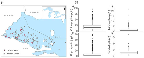
Figure 1.
(I) Ground samples distributed in the Western Lake Erie basin. The location map shows Lake Erie as part of the Great Lakes Basin. (II) Boxplot of the values for algal bloom proxies (a) Chlorophyll-a, (b) Phycocyanin, (c) Microcystin, and (d) Secchi-depth. The box indicates the interquartile range, i.e., 25–75 percentile and the line inside the box shows the median. The dots following the whisker (error bar) represent the outliers.
2.2. Datasets
2.2.1. Sentinel-3A OLCI Level-2 Dataset
This study uses OLCI Level-2 Water Full Resolution (OL_2_WFR) data product from Sentinel-3A, a satellite that was launched in February 2016 and is currently operational [47]. We focused on the period between 2016 and 2021. OLCI sensor on Sentinel-3A provides multi-channel spectral measurements for land and water surfaces at a spatial resolution of 300 m and a daily temporal frequency [48,49]. Specifically, it comprises a wide range of 21 spectral bands, covering visible to near-infrared regions (400 nm to 1020 nm) of the wavelength spectrum [47]. In addition, OLCI has a channel at 1.02 µm to improve the atmospheric correction and another at 673 nm for better observations of Chlorophyll fluorescence [50].
The OLCI Level-2 product, which was reprocessed based on the latest standards, was accessed from two sources. One of them was Copernicus Online Data Access CODA web portal (https://user.eumetsat.int/data-access/data-centre, accessed on 1 August 2022) which provides data on a one-year rolling archive basis while data older than a year were retrieved from EUMETSAT Data Center [51]. The final Level-2 product includes 16 bands excluding bands 13, 14, 15, 19, and 20 which are meant to be used for measuring atmospheric gas absorption [52].
2.2.2. Ground-Based Station Datasets
For a study period of 2016 through 2021, in-situ data for four proxies, Chl-a, PC, MC, and SD, were compiled from two ground-based monitoring programs, one conducted by National Oceanic and Atmospheric Administration Great Lakes Environmental Research Laboratory (NOAA GLERL) and another by Ohio Sea Grant Stone Lab Algal and Water Quality Laboratory (https://ohioseagrant.osu.edu/research/live/water, accessed on 5 August 2022). The distribution of the measurements in the study area is illustrated in Figure 1. Among the ground samples that matched with the satellite images, 240 were collected from NOAA GLERL while the rest 127 samples were from Stone Lab Algal and Water Quality Laboratory. A sample of a raw Sentinel-3A image, along with the distribution of Chl-a, PC, MC, and SD for the same date overlaid on the Sentinel-3 image, can be found in the Supporting Document (Figure S1).
The water quality monitoring of the western basin of Lake Erie started in 2012, with the collaboration between the NOAA GLERL, the Cooperative Institute for Great Lakes Research (CIGLR), and the University of Michigan (UM). CIGLR deployed buoys to gather in situ observations that involve the parameters like wind speed, depth, water temperature, turbidity, dissolved oxygen, Chl-a, PC, nitrate, and phosphate through recurring weekly sampling trips to a set of stations before, during, and after HAB events (from May–October) [53]. The physical, chemical, and biological water quality data are available through Water Quality and Buoy Data Portal (https://www.glerl.noaa.gov/res/HABs_and_Hypoxia/habsMon.html, accessed on 5 August 2022).
Datasets from Ohio Sea Grant Stone Lab, also commonly called “Charters Captain” datasets, are collected by charter boat captains and aboard Stone Lab science cruises using a surface-to-2-m intergraded tube sampler under the support of Ohio EPA Environmental Education Fund and Surface Water Improvement Fund [54]. The samples are analyzed in the laboratory to detect the presence of water quality indicators namely, Chl-a (an indicator of algal biomass), MC (a toxin generated by cyanobacteria), total suspended solids (mass of all particulates in the water), total phosphorus and nitrogen (indicators of maximum biomass potential), dissolved nitrate, phosphate, and silicate (nutrients accessible for algae) while the ancillary datasets like GPS location, water temperature, and Secchi disk depth (an indicator of water clarity) are also recorded. The dataset holds water quality information from 2013 to 2022 and can be accessed through Stone Lab Algal and Water Quality Laboratory website (https://ohioseagrant.osu.edu/research/live/water, accessed on 5 August 2022).
2.3. Cyanobacteria Proxies
Chl-a is a primary photosynthetic pigment in phytoplankton (or algae) and is thus considered a proxy for the bloom [55,56]. Since it is a general measure of identification for all phytoplankton, it can be less useful in categorizing distinct phytoplankton species. Phycocyanin (PC) is another type of photo-pigment widely found in cyanobacteria and thus it can be useful in measuring pigments specific to cyanobacteria [30]. Even though it may not be as effective as Chl-a at low cyanobacterial biomass, the implicit link between remotely-sensed PC and the toxicity of the algal group can provide important information about any potential harm [57].
While Chl-a and PC indicate the presence of cyanobacterial bloom, MC indicates cyanotoxins that are seen in cyanobacterial blooms [28,56]. However, MC comes with poor optical sensitivity. With the waters that is heavily infested with cyanobacteria, [58] suggested that high algal biomass represented by high Chl-a concentration could indicate the chances of high cyanotoxin concentration. As such, MC has commonly been explained based on its relationship with Chl-a and PC [59,60].
In addition to the chemical parameters mentioned above, Secchi depth (SD), a physical parameter indicating water clarity, is estimated based on how light is absorbed and scattered by the water and, consequently, how deep it may penetrate the water [61]. Most often, excessive presence of bloom at the water body surface hinders the penetration of light, consequently, affecting the SD [62,63]. Primarily, SD is more indicative of water clarity than the bloom itself and is influenced by various factors such as suspended inorganic particles, colored dissolved organic matter (CDOM), and the resuspension of bottom sediments. It is one of the simple yet inexpensive method to provide a reasonable estimate of bloom [64]. When used in conjunction with other chemical parameters like Chl-a, it can offer a better understanding of the bloom phenomenon. Therefore, an empirical correlation between SD and Chl-a has been established, as Chlorophyll is the dominant attenuating substance in the bloom [61].
2.4. Data Quality Control
Before analyzing the collected ground samples, a quality control process was conducted to ensure the accuracy and reliability of the dataset. Certain criteria were followed in filtering the datasets. Since the use of clouded pixels hinders the interpretation of the details, the ground samples for which the corresponding reflectance (pixel) values from Sentinel-3 OLCI images were flagged as cloud-ambiguous or cloud margins, were discarded. Similarly, to ensure that only near-surface samples are considered, samples collected at depths greater than 0.5 m were not taken into consideration. Additionally, to avoid the mixed pixel effect, samples collected within or less than 300 m (the pixel size of OLCI images), were removed. Furthermore, the ground samples collected from shallow waters along the shoreline were ignored as the reflection of light off the waterbed can interfere with the accuracy of the measurements. Moreover, the negative values of the proxies in ground-collected samples were considered outliers and hence discarded. For further analysis, a total of 367 ground-based samples that matched the OLCI images were taken into consideration.
2.5. Spatial Matchups
To accurately identify spatial matchups, satellite overpasses that were in close proximity to in situ measurements sites, both geographically temporally, were considered. This approach ensures that the satellite data and the ground-based observations are comparable. Given the large pixel size and significant variability observed even within a short distance, a single pixel from the satellite data containing the station coordinates were selected. By focusing on one specific pixel, potential discrepancies arising from spatial heterogeneity are minimized, thereby enhancing the reliability of the comparative analysis.
3. Methods
The overall workflow considered in the study is illustrated in Figure 2. This involves the compilation of water quality proxies from ground datasets and band reflectance from Sentinel-3, followed by data preparation and pre-processing to train and validate four RF models, with each model per proxy.
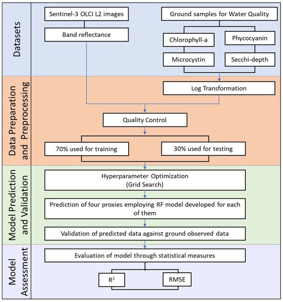
Figure 2.
Flowchart showing the different stages of working methodology involving acquisition of datasets, data preparation and pre-processing, model prediction and validation, and model assessment.
3.1. Overview of the Algorithm: Random Forest
This study utilized the RF model, a well-known ensemble learning method, to assess Chl-a, PC, MC, and SD. It has been used for a wide variety of applications for its ability to depict the nonlinear effect of involved variables and its robustness to outliers [8,41,65]. In addition, the ability to assess the relative importance of the predictor variables and identify the most relevant ones helps reduce the dimension of the model [31]. The RF is built on multiple decision trees, each of which is trained on a subset of the input variable set, which is randomly chosen at each node known as feature bagging [66,67,68]. Hence, an uncorrelated forest of decision trees is produced by incorporating randomness into the model. The RF regression model averages the results of these decision trees to make the final prediction [67]. The averaging out of uncorrelated trees helps in bringing down the variance, therefore reducing the chances of overfitting. In this study, the models were trained on 70% (257 samples) of the datasets, while the rest 30% (110 samples) were used in testing the performance of the model.
In the model, while 16 spectral bands act as predictors, four HAB proxies (i.e., Chl-a, MC, PC, and SD) act as the response variables. To address the skewness and heteroscedasticity exhibited by the residuals of response variables, they are log-transformed before being used in the model. As an example, Figure 3 shows the transformation of Chl-a measurements to a log-normal distribution.
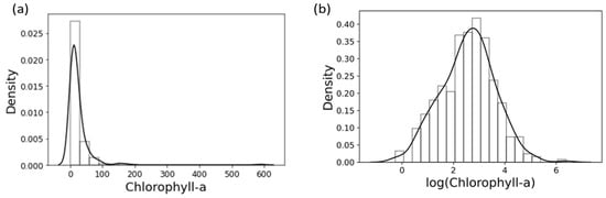
Figure 3.
Histogram with a fitted density curve represented by a solid black line for Chlorophyll-a (a) Before and (b) After log-transformation.
The RF models were built using the scikit-learn machine learning library in a Python environment. The model was tuned using four hyperparameters, including maximum depth, minimum sample leaf, minimum leaf split, and the number of regression trees (also referred to as N_estimator), to optimize the model performance. To automate the process of identifying an optimal combination of hyperparameters values that offers the best RF model performance, the function GridSearchCV from scikit-learn was implemented. It carries out k-fold cross-validation internally for every set of hyperparameters. Specifically, the dataset is divided into k folds. The model is then trained on k-1 folds and validated on the remaining fold. This process is repeated k times. The performance is averaged over all folds to determine which combination of hyperparameters yields the highest performance [68]. In this study, GridSearchCV used 5-fold cross-validation. Table 1 lists hyperparameters obtained from GridSearchCV, utilized for each of the three response variables in the RF models.

Table 1.
Hyperparameters used for the random forest modeling.
The relative importance of each band in the model was derived from the built-in feature importance method for Random Forest available in Scikit-learn library in python. The values inherited from the importance table are helpful in understanding that not all the bands substantially affect the prediction in the model. Therefore, sensitivity analysis was conducted to assess how the model’s performance varied with different combinations of bands. For the sensitivity analysis, all the predictor variables were present at the beginning of the model run, followed by successive elimination of the predictor variable with the lowest relative importance to a given response variable from the model. This process was done for all four proxies. Further, the relationship between the number of spectral bands used in the model and the model performance was assessed.
3.2. Model Performance Assessment
To assess the performance of the RF models, two metrics, including root mean square error (RMSE) and coefficient of determination (R2), were used on the testing dataset (Equations (1) and (2)). In the equations, is the measured value for ith observation, is the predicted values for corresponding to the , while is the average of y with N number of samples.
Since the dependent variables are subjected to logarithmic transformation while fitting into the model, the predictions were transformed back to their original range before calculating the error metrics that involve them. Since a straightforward method of taking an antilog would essentially add a bias during back transformation, the back-transformed estimates are multiplied by an exponential of half the variance of transformed variable errors [69,70].
Relationship between Chl-a, PC, MC, and SD were further assessed as they reflect similar behaviors in some band spectrums. Given the easier detection of Chl-a compared to other proxies, Chl-a could be used as a stand-in for other proxies representing the harmful algal bloom. Since the RF models underperformed with the low concentrations of proxies, the relationship between Chl-a and other proxies during peak bloom periods with warm temperatures and comparatively high concentrations were investigated. Similar analysis was conducted in prior work [71]. Specifically, for the study period of 2016 to 2021, monthly average of proxies from April through October were examined.
4. Results
4.1. Model Prediction and Feature Importance
The RF model estimates for Chl-a, PC, MC, and SD in relation to ground observations for the test dataset are illustrated in Figure 4. Chl-a showed the highest prediction accuracy, with the RF model explaining 55% of the variability and an RMSE of 20.84 µg/L. Followed by Chl-a are SD (R2 = 0.47 and RMSE = 0.71 m), PC (R2 = 0.46 and RMSE = 70.92 µg/L), and MC (R2 = 0.44 and RMSE = 3.39 µg/L), all with the comparable performances. Section 4.2 delves deeper into the relationships between these proxies.
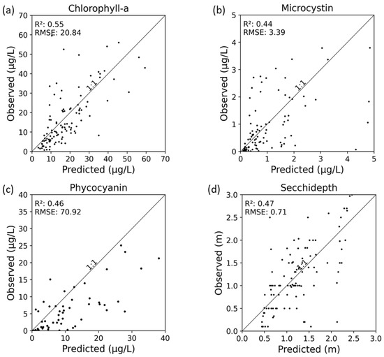
Figure 4.
Predicted and observed values for (a) Chlorophyll-a, (b) Microcystin, (c) Phycocyanin, and (d) Secchi-depth.
To determine the importance of 16 spectral bands on the prediction of each proxy, they were ranked based on their relative importance as illustrated in Figure 5. Among 16 bands, Band 04 peaked with a large fold for three out of four proxies, Chl-a, PC, and MC. In addition to Band 04, Chl-a was also influenced by a few other bands, including Bands 16, 11, 21, and 03. Similar to Chl-a, Bands 04, 03, and 11 were the most influential for PC when all bands were included. Like Chl-a, Band 04 among all other bands showed a high importance for MC. This illustrated how, despite MC’s lower sensitivity to optical sensors, it was correlated with Chl-a. Contrarily, for the SD model, spectral Bands 12, followed by 16 and 11 played the most important role, unlike the rest of other proxies.
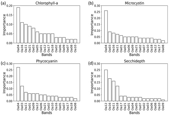
Figure 5.
Ranking of the relative importance of 16 bands which are predictor estimates of HAB proxies (a) Chlorophyll-a, (b) Microcystin, (c) Phycocyanin, and (d) Secchi-depth. The OLCI bands are represented by “Oa” followed by the band number.
The sensitivity analyses indicated that RMSE and R2 remained relatively stable for Chl-a until 10 bands were dropped and only 6 were included in the model (Figure 6). Similarly, the use of 10 bands as predictors yielded the highest R2 and lowest RMSE for both PC and MC, while some spikes and falls were observed after the saturation point. For example, a significant decrease in R2 was observed for MC after the number of bands dropped from 10 to 8, but the change in RMSE was not as pronounced. Among four different proxies, SD required a larger number of predictors (13 bands) to reach tentative saturation compared to other proxies. All proxies showed a sharp decrease in R2 as the number of bands reduced to 2–4, while the corresponding changes in RMSE were less pronounced. The overall result confirmed that eliminating a certain number of bands yielded the best statistical performances for all the proxies.
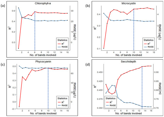
Figure 6.
Variation of statistical metrics with respect to the number of predictor variables for (a) Chlorophyll-a, (b) Microcystin, (c) Phycocyanin, and (d) Secchi-depth at each step through the elimination procedure. The dotted blue vertical lines denote the tentative saturation levels of both metrics.
4.2. Association of MC, PC, and SD with Chl-a
PC and MC tend to emulate the nature of Chl-a as demonstrated by the similar trend in monthly averages across all years (Figure 7). Notably, with an increase in algal mass in water, the concentration of Chl-a increases while there is a corresponding decrease in SD This inverse relationship of SD with all the other proxies was observed in most months except when the graph transcends from April to May and September to October. Also, in September, the anticipated positive association between Chl-a and MC was not observed.
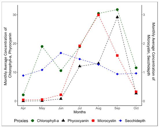
Figure 7.
Monthly average concentration of the proxies across the years 2016 through 2021 for the months of April through October (months witnessing the highest algal blooms).
When proxies were analyzed for the peak bloom months, there was a relatively strong linear relationship between Chl-a and MC with R2 = 0.83 (Figure 8a). The observed linear relationship provided further evidence of the strong affinity between MC and Chl-a, in addition to the previously noted strong model accuracy of MC and its ability to mimic the band importance of Chl-a. The linear relationship of PC in Figure 8b was poorer than MC with Chl-a explaining only 34% of the variance in PC. On the other hand, a peculiar hyperbolic relationship between Chl-a and SD could be observed where Chl-a was able to explain 30% of variance present in SD. With Chl-a concentration less than 50 µg/L, the SD indicated a decline, after which it saturated as the Chl-a increased. Since the number of Chl-a observations greater than 50 µg/L is low, the relationship between SD and Chl-a values in the higher Chl-a concentration range could not be discerned.
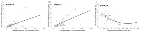
Figure 8.
Linear regression of Chlorophyll-a with (a) Microcystin (b) Phycocyanin and (c) Non-linear polynomial regression with Secchi-depth, respectively. The solid black lines represent the best fit of the regression models.
5. Discussion
Prior studies have investigated various models that employ different combinations of spectral bands, such as two bands, three bands, or multiple band ratios, to estimate Chl-a concentrations in water bodies. For instance, for Chl-a estimation, there are studies that used a three-band model incorporating MERIS spectral bands (660–670 nm, 703.75–713.75 nm, and 750–757.5 nm) and the 2-band model with MODIS spectral bands (662–672 nm and 743–753 nm) [72], while some experimented with multiple band ratios (e.g., green-blue band ratios, green-red band ratio, NIR-red band ratios, and three-band ratio) [73]. Unlike these studies, this study incorporated all the available 16 spectral bands in RF models to capture the potential subtle variations in the spectral signature to predict HAB proxies. Specifically, a RF model was employed for each of the four proxies, and the results demonstrated varying levels of prediction accuracy. Notably, Chl-a exhibited the highest predictability compared to other proxies. It could be attributed to the fact that Chl-a has a higher dominance on harmful algae as compared to other variables. Compared to Chl-a, PC is usually less prevalent in the bloom and in this study, PC concentration used was very low (less than 10 µg/L), resulting in relatively low variability. On the other hand, MC, despite being a chemical toxin that is hard to detect through remote sensing, and SD being a coarse measure of water quality still depicted performances similar to PC.
5.1. Model Prediction and Feature Importance
In the study, the prediction model for Chl-a showed the highest accuracy compared to three other proxies. It could be attributed to Chl-a’s higher dominance in harmful algal blooms. Compared to Chl-a, PC is less prevalent in blooms, and its concentration in this study was below 10 µg/L (Figure 8b). This could be linked to lower sensitivity and poor model performance. Similar behavior was found in the study carried out by [74] where PC estimates retrieved from field radiometric and pigment data collected over the Netherlands and Spain had the highest errors for PC levels lower than 50 µg/L. Another study that used Sentinel-3 imagery suggested that the inclusion of datasets with the majority of PC concentrations lower than 10 µg/L and Chl-a concentrations lower than 50 µg/L may have influenced the models’ subpar performance [21]. Employing semi-empirical algorithms, they achieved maximum R2 of 0.136 and 0.163 for PC and Chl-a respectively.
In the study, we included 16 spectral bands as predictor variables for each of the four proxies, aiming to analyze the efficacy of each band in explaining variability in the bloom proxies. However, it’s important to note that when we analyzed the importance of these 16 spectral bands in predicting each proxy (Figure 6), we observed that a reduced number of bands may be sufficient to achieve acceptable model performance. This finding could have implications for data acquisition and processing in future application.
The importance of spectral bands, including Band 03 (442.5 nm), Band 04 (490 nm), Band 11 (708.75 nm), Band 16 (778.75 nm), and Band 21 (1020 nm), in predicting Chl-a can be attributed to the role of Chl-a as a major light-harvesting pigment involved in photosynthesis for algal masses [17]. Band 04 is situated at the borderline of the blue and green regions, Band 11 falls within red, and Band 16 and Band 21 belong to the infrared region. This highlights the distinctive trait of Chl-a, which shows low reflectance in the blue-green region and high absorption in the red and near-infrared region [52,75,76]. A recent study [77] evaluating the satellite-based algorithm for detecting cyanobacteria blooms found that PC absorption at 620 nm is two to three times lower than that of Chl-a. This means it takes two to three times the concentration of PC to achieve the same sensitivity as compared to Chl-a. In this study, low PC concentration likely led the model to prioritize Band 03 and Band 04 over Band 07. In general, a high abundance of phytoplankton species that outcompete the cyanobacteria could lead to a low PC concentration. In such situation, there are less pigment molecules to absorb the incoming light and as a result, less light gets absorbed by the sample causing lower signal in the spectral bands that correspond to the absorption of PC [78].
The better modeling for MC and SD observed in this study could be linked to their relationship with Chl-a, which has higher sensitivity to the spectral bands used. Prior works suggest that MC does not exhibit a strong affinity for specific spectral bands within the visible or near-infrared regions, unlike Chl-a and PC [29,58,77]. But we observed similar results between MC and Chl-a in the scatter plot showing the model performance (Figure 4) and the feature importance table (Figure 5). Therefore, it is plausible that a significant portion of the spectral characteristics displayed by MCs is due to their interaction with Chl-a. The relationship between these two proxies is discussed further in Section 5.2.
Spectral bands (i.e., Band 11, 12, 16, and 18) in red and NIR regions were found to be important in explaining variability in SD. Blooms strongly absorb light in the red and NIR regions [79], and SD typically has an inverse relationship with bloom biomass [62,80]. This implies that the deeper the SD, the lower the bloom and thus higher the reflectance in the red and NIR bands. Based on this potential relationship between the bloom and SD, prior works have used red and NIR bands of satellite images to estimate SD [81,82,83]. This suggests that in the absence of proxies like Chl-a, PC, and MC, SD could also be employed to estimate the spatial and temporal extent of algal blooms in water resources.
5.2. Temporal Association between the Parameters
HABs in the Lake Erie basin are normally expected to reach the peak bloom sometime between July to October [84]. Therefore, the association between Chl-a with other proxies (i.e., PC, MC, and SD) was examined for the peak bloom months of August and September to shed light on the significance of combining multiple proxies to guide bloom monitoring. A strong linear relationship between Chl-a and MC with R2 of 0.83 observed in the study (Figure 8a), suggests that a considerable portion of the Chl-a can explain the presence of HABs, as it is strongly associated with MC. While the information on Chl-a alone does not suffice to explain the presence of HAB as Chl-a is present in many other phytoplankton species, incorporating the information from different proxies elevates the applicability of Chl-a in determining the presence of the bloom.
The closeness in the trend of Chl-a and PC in the monthly averages (Figure 7) demonstrates the affinity between these two pigments. For some months, such as May, Chl-a increased significantly but not PC, suggesting that the increase in Chl-a may have been due to phytoplankton biomass rather than algal blooms. Despite their similar monthly trends, the weak linkage between Chl-a and PC (Figure 8b) can be attributed to the low mean concentration of PC (Section 5.1).
An exponential decline in SD with increasing Chl-a (Figure 8c) suggests the inverse relationship between SD and Chl-a. It was observed that, at Chl-a concentrations below 50 µg/L, even a small change in Chl-a concentration resulted in substantial changes in SD. For instance, increasing Chl-a concentration from 0 µg/L to 10 µg/L resulted in a total decrease of 0.41 m in SD (from 1.97 m to 1.56 m). However, the change in SD became less significant as the Chl-a concentration increased above 50 µg/L, where a change in Chl-a concentration from 50 µg/L to 60 µg/L led to a total change in SD of just 0.09 m (from 0.54 m to 0.45 m). These observed relationships between Chl-a and SD suggest that a Chl-a concentration of 50 µg/L could serve as a threshold for using SD as a water quality metric in bloom-affected areas. Conversely, SD is not an effective proxy of changes in algal blooms in eutrophic waters with Chl-a values above 50 µg/L, where SD and Chl-a are barely related to each other.
The findings from each of the proxies highlight the importance of incorporating complementary measures, such as MC, PC, and SD as opposed to using only a common proxy like Chl-a, to give a clear picture of the bloom. The analysis from this study could offer a strong foundation that can be extended to future research using multiple proxies in determining the existence of bloom. Additionally, incorporating hydrometeorological conditions, such as temperature, precipitation, and wind, can enhance bloom monitoring by accounting for their significant influence on bloom behavior.
Overall, interpretability obtained from RF algorithm offered valuable insights into the relative importance of different predictor variables, supporting more informed decision-making for bloom presence and thereby, water resource management. Our study demonstrates the benefits of using advanced machine learning, specifically RF with Sentinel-3 OLCI satellite imagery, for efficient HAB monitoring, especially in situations where acquiring real-time in-situ data across different spatial scales is immensely challenging. Future research could enhance predictive capabilities by integrating more machine learning algorithms and multispectral data sources.
6. Conclusions
This study leveraged high-frequency multispectral Sentinel-3 satellite imageries to identify HAB proxies in response to their distinctive spectral characteristics. Based on the performance of RF models curated for four proxies of algal bloom and the assessment of spectral bands used in model development, proxies were found to be specifically more sensitive to blue-green, red, and infrared regions. The RF model for Chl-a explained variability in ground-truth data more strongly (R2 = 0.55 and RMSE = 20.84 µg/L) as compared to the RF models for MC (R2 = 0.44 and RMSE = 3.39 µg/L), PC (R2 = 0.46 and RMSE = 70.92 µg/L), and SD (R2 = 0.47 and RMSE = 0.71 m). MC, which is hard to detect using only spectral information, was found to closely imitate the behavior of Chl-a. The link between Chl-a and MC, given that MC is the toxic component of the bloom, could help identify the existence of toxic cyanobacterial blooms from the non-toxic blooms. Similarly, the association of SD and Chl-a can help establish an ecological bloom threshold for the use of SD as a metric of water quality in bloom-affected waters. However, due to PC’s low concentration, it did not exhibit a strong relationship with Chl-a. With four proxies involved in explaining the bloom phenomena, the correlation between them suggests that utilizing multiple proxies can offset the disadvantages of one proxy with the advantages of the other. Overall, leveraging the satellite data alongside the available proxies indicating the bloom, hold immense potential for generating valuable insights that can assist in the development of effective mitigation measures against the nuisance caused by toxic algal bloom.
Supplementary Materials
The following supporting information can be downloaded at: https://www.mdpi.com/article/10.3390/rs16132444/s1, Figure S1. Raw Sentinel 3A OLCI image in the background from June 22, 2021; Figure S2. Model performances (R2 and RMSE) for five random sets of samples from the dataset.
Author Contributions
Conceptualization, S.K. and K.Z.; methodology, N.J., S.K., K.Z. and J.P.; software, N.J.; validation, N.J., S.K., K.Z. and J.P.; formal analysis, N.J.; investigation, N.J.; resources, S.K.; data curation, N.J. and A.L.; writing—N.J.; writing—review and editing, S.K., K.Z. and J.P.; visualization, N.J.; supervision, S.K., K.Z. and J.P.; project administration, S.K.; funding acquisition, S.K. and K.Z. All authors have read and agreed to the published version of the manuscript.
Funding
This work was partially funded by a Harmful Algal Bloom Research Initiative grant from the Ohio Department of Higher Education (#GR119061) and the OSU Graduate School Fellowship programs, including College Allocated and Environmental Fellowships.
Data Availability Statement
Sentinel-3 OLCI data can be downloaded from CODA (Copernicus Online Data Access) Web Service (https://coda.eumetsat.int/, accessed on 1 August 2022) and the data older than a year are stored in a rolling archive accessible in https://www.eumetsat.int/website/home/Data/DataDelivery/EUMETSATDataCentre/index.html (accessed on 1 August 2022). The ground-based water quality dataset can be downloaded from https://ohioseagrant.osu.edu/research/live/water (accessed on 5 August 2022).
Conflicts of Interest
Neha Joshi is employed by Arcadis U.S., Inc. The authors declare no conflict of interest.
References
- Ho, J.C.; Michalak, A.M. Challenges in Tracking Harmful Algal Blooms: A Synthesis of Evidence from Lake Erie. J. Great Lakes Res. 2015, 41, 317–325. [Google Scholar] [CrossRef]
- Nemes, J. Ohio EPA Declares Western Lake Erie Impaired. Environmental Law & Policy Center: Chicago, IL, USA, 2018. Available online: https://elpc.org/blog/ohio-epa-declares-western-lake-erie-impaired/ (accessed on 26 October 2022).
- Mohamed, M.N.; Wellen, C.; Parsons, C.T.; Taylor, W.D.; Arhonditsis, G.; Chomicki, K.M.; Boyd, D.; Weidman, P.; Mundle, S.O.C.; Van Cappellen, P.; et al. Understanding and managing the re-eutrophication of Lake Erie: Knowledge gaps and research priorities. Freshw. Sci. 2019, 38, 675–691. [Google Scholar] [CrossRef]
- Watson, S.B.; Miller, C.; Arhonditsis, G.; Boyer, G.L.; Carmichael, W.; Charlton, M.N.; Confesor, R.; Depew, D.C.; Höök, T.O.; Ludsin, S.A.; et al. The Re-Eutrophication Of Lake Erie: Harmful Algal Blooms and Hypoxia. Harmful Algae 2016, 56, 44–66. [Google Scholar] [CrossRef] [PubMed]
- Caballero, I.; Fernández, R.; Escalante, O.M.; Mamán, L.; Navarro, G. New Capabilities of Sentinel-2A/B Satellites Combined with in Situ Data for Monitoring Small Harmful Algal Blooms in Complex Coastal Waters. Sci. Rep. 2020, 10, 8743. [Google Scholar] [CrossRef] [PubMed]
- Izadi, M.; Sultan, M.; Kadiri, R.E.; Ghannadi, A.; Abdelmohsen, K. A Remote Sensing and Machine Learning-Based Approach to Forecast the Onset of Harmful Algal Bloom. Remote Sens. 2021, 13, 3863. [Google Scholar] [CrossRef]
- Yang, H.; Kong, J.; Hu, H.; Du, Y.; Gao, M.; Chen, F. A Review of Remote Sensing for Water Quality Retrieval: Progress and Challenges. Remote Sens. 2022, 14, 1770. [Google Scholar] [CrossRef]
- Douna, V.; Barraza, V.; Grings, F.; Huete, A.; Restrepo-Coupe, N.; Beringer, J. Towards a Remote Sensing Data Based Evapotranspiration Estimation in Northern Australia Using a Simple Random Forest Approach. J. Arid Environ. 2021, 191, 104513. [Google Scholar] [CrossRef]
- Rubin, H.J.; Lutz, D.A.; Steele, B.G.; Cottingham, K.L.; Weathers, K.C.; Ducey, M.J.; Palace, M.; Johnson, K.M.; Chipman, J.W. Remote Sensing of Lake Water Clarity: Performance and Transferability of Both Historical Algorithms and Machine Learning. Remote Sens. 2021, 13, 1434. [Google Scholar] [CrossRef]
- Wen, J.; Yang, J.; Li, Y.; Gao, L. Harmful Algal Bloom Warning Based on Machine Learning in Maritime Site Monitoring. Knowl.-Based Syst. 2022, 245, 108569. [Google Scholar] [CrossRef]
- Zhang, F.; Hu, C.; Shum, C.K.; Liang, S.; Lee, J. Satellite Remote Sensing of Drinking Water Intakes in Lake Erie for Cyanobacteria Population Using Two MODIS-Based Indicators as a Potential Tool for Toxin Tracking. Front. Mar. Sci. 2017, 4, 124. [Google Scholar] [CrossRef]
- Klemas, V. Remote Sensing of Algal Blooms: An Overview with Case Studies. J. Coast. Res. 2012, 28, 34–43. [Google Scholar] [CrossRef]
- Shen, L.; Xu, H.; Guo, X. Satellite Remote Sensing of Harmful Algal Blooms (HABs) and a Potential Synthesized Framework. Sensors 2012, 12, 7778–7803. [Google Scholar] [CrossRef]
- Stumpf, R.P.; Culver, M.E.; Tester, P.A.; Tomlinson, M.; Kirkpatrick, G.J.; Pederson, B.A.; Truby, E.; Ransibrahmanakul, V.; Soracco, M. Monitoring Karenia Brevis Blooms in the Gulf of Mexico Using Satellite Ocean Color Imagery and Other Data. Harmful Algae 2003, 2, 147–160. [Google Scholar] [CrossRef]
- Rodríguez-Benito, C.V.; Navarro, G.; Caballero, I. Using Copernicus Sentinel-2 and Sentinel-3 Data to Monitor Harmful Algal Blooms in Southern Chile during the COVID-19 Lockdown. Mar. Pollut. Bull. 2020, 161, 111722. [Google Scholar] [CrossRef]
- Urquhart, E.A.; Schaeffer, B.A. Envisat MERIS and Sentinel-3 OLCI Satellite Lake Biophysical Water Quality Flag Dataset for the Contiguous United States. Data Br. 2020, 28, 104826. [Google Scholar] [CrossRef]
- Ali, K.; Witter, D.; Ortiz, J. Application of Empirical and Semi-Analytical Algorithms to MERIS Data for Estimating Chlorophyll a in Case 2 Waters of Lake Erie. Environ. Earth Sci. 2014, 71, 4209–4220. [Google Scholar] [CrossRef]
- Matthews, M.W.; Bernard, S.; Winter, K. Remote Sensing of Cyanobacteria-Dominant Algal Blooms and Water Quality Parameters in Zeekoevlei, a Small Hypertrophic Lake, Using MERIS. Remote Sens. Environ. 2010, 114, 2070–2087. [Google Scholar] [CrossRef]
- Seegers, B.N.; Werdell, P.J.; Vandermeulen, R.A.; Salls, W.; Stumpf, R.P.; Schaeffer, B.A.; Owens, T.J.; Bailey, S.W.; Scott, J.P.; Loftin, K.A. Satellites for Long-Term Monitoring of Inland U.S. Lakes: The MERIS Time Series and Application for Chlorophyll-A. Remote Sens. Environ. 2021, 266, 112685. [Google Scholar] [CrossRef]
- Cherif, E.K.; Mozetič, P.; Francé, J.; Flander-Putrle, V.; Faganeli-Pucer, J.; Vodopivec, M. Comparison of In-Situ Chlorophyll-a Time Series and Sentinel-3 Ocean and Land Color Instrument Data in Slovenian National Waters (Gulf of Trieste, Adriatic Sea). Water 2021, 13, 1903. [Google Scholar] [CrossRef]
- Ogashawara, I. The Use of Sentinel-3 Imagery to Monitor Cyanobacterial Blooms. Environments 2019, 6, 60. [Google Scholar] [CrossRef]
- Pirasteh, S.; Mollaee, S.; Narges Fatholahi, S.; Li, J. Estimation of Phytoplankton Chlorophyll-a Concentrations in the Western Basin of Lake Erie Using Sentinel-2 and Sentinel-3 Data. Can. J. Remote Sens. 2020, 46, 585–602. [Google Scholar] [CrossRef]
- Binding, C.E.; Greenberg, T.A.; McCullough, G.; Watson, S.B.; Page, E. An Analysis of Satellite-Derived Chlorophyll and Algal Bloom Indices on Lake Winnipeg. J. Great Lakes Res. 2018, 44, 436–446. [Google Scholar] [CrossRef]
- Papenfus, M.; Schaeffer, B.; Pollard, A.I.; Loftin, K. Exploring the Potential Value of Satellite Remote Sensing to Monitor Chlorophyll-a for US Lakes and Reservoirs. Environ. Monit. Assess. 2020, 192, 1–22. [Google Scholar] [CrossRef]
- Khan, R.M.; Salehi, B.; Mahdianpari, M.; Mohammadimanesh, F.; Mountrakis, G.; Quackenbush, L.J. A Meta-Analysis on Harmful Algal Bloom (Hab) Detection and Monitoring: A Remote Sensing Perspective. Remote Sens. 2021, 13, 4347. [Google Scholar] [CrossRef]
- Beck, R.; Xu, M.; Zhan, S.; Johansen, R.; Liu, H.; Tong, S.; Yang, B.; Shu, S.; Wu, Q.; Wang, S.; et al. Comparison of Satellite Reflectance Algorithms for Estimating Turbidity and Cyanobacterial Concentrations in Productive Freshwaters Using Hyperspectral Aircraft Imagery and Dense Coincident Surface Observations EPA Public Access. J. Great Lakes Res. 2019, 45, 413–433. [Google Scholar] [CrossRef]
- Kuhn, C.; de Matos Valerio, A.; Ward, N.; Loken, L.; Sawakuchi, H.O.; Kampel, M.; Richey, J.; Stadler, P.; Crawford, J.; Striegl, R.; et al. Performance of Landsat-8 and Sentinel-2 Surface Reflectance Products for River Remote Sensing Retrievals of Chlorophyll-a and Turbidity. Remote Sens. Environ. 2019, 224, 104–118. [Google Scholar] [CrossRef]
- Liu, Q.; Rowe, M.D.; Anderson, E.J.; Stow, C.A.; Stumpf, R.P.; Johengen, T.H. Probabilistic Forecast of Microcystin Toxin Using Satellite Remote Sensing, in Situ Observations and Numerical Modeling. Environ. Model. Softw. 2020, 128, 104705. [Google Scholar] [CrossRef]
- Francy, D.S.; Brady, A.M.G.; Stelzer, E.A.; Cicale, J.R.; Hackney, C.; Dalby, H.D.; Struffolino, P.; Dwyer, D.F. Predicting Microcystin Concentration Action-Level Exceedances Resulting from Cyanobacterial Blooms in Selected Lake Sites in Ohio. Environ. Monit. Assess. 2020, 192, 1–27. [Google Scholar] [CrossRef] [PubMed]
- McHau, G.J.; Makule, E.; Machunda, R.; Gong, Y.Y.; Kimanya, M. Phycocyanin as a Proxy for Algal Blooms in Surface Waters: Case Study of Ukerewe Island, Tanzania. Water Pract. Technol. 2019, 14, 229–239. [Google Scholar] [CrossRef]
- Zolfaghari, K.; Pahlevan, N.; Binding, C.; Gurlin, D.; Simis, S.G.H.; Verdu, A.R.; Li, L.; Crawford, C.J.; Vanderwoude, A.; Errera, R.; et al. Impact of Spectral Resolution on Quantifying Cyanobacteria in Lakes and Reservoirs: A Machine-Learning Assessment. IEEE Trans. Geosci. Remote Sens. 2022, 60, 1–20. [Google Scholar] [CrossRef]
- Chang, K.W.; Shen, Y.; Chen, P.C. Predicting Algal Bloom in the Techi Reservoir Using Landsat TM Data. Int. J. Remote Sens. 2010, 25, 3411–3422. [Google Scholar] [CrossRef]
- Çamdevýren, H.; Demýr, N.; Kanik, A.; Keskýn, S. Use of Principal Component Scores in Multiple Linear Regression Models for Prediction of Chlorophyll-a in Reservoirs. Ecol. Modell. 2005, 181, 581–589. [Google Scholar] [CrossRef]
- Yu, P.; Gao, R.; Zhang, D.; Liu, Z.P. Predicting Coastal Algal Blooms with Environmental Factors by Machine Learning Methods. Ecol. Indic. 2021, 123, 107334. [Google Scholar] [CrossRef]
- Ly, Q.V.; Nguyen, X.C.; Lê, N.C.; Truong, T.D.; Hoang, T.H.T.; Park, T.J.; Maqbool, T.; Pyo, J.C.; Cho, K.H.; Lee, K.S.; et al. Application of Machine Learning for Eutrophication Analysis and Algal Bloom Prediction in an Urban River: A 10-Year Study of the Han River, South Korea. Sci. Total Environ. 2021, 797, 149040. [Google Scholar] [CrossRef] [PubMed]
- Prasad, S.; Saluja, R.; Garg, J.K. International Journal of Remote Sensing Assessing the Efficacy of Landsat-8 OLI Imagery Derived Models for Remotely Estimating Chlorophyll-a Concentration in the Upper Ganga River, India Assessing the Efficacy of Landsat-8 OLI Imagery Derived Models for R. Int. J. Remote Sens. 2020, 41, 2439–2456. [Google Scholar] [CrossRef]
- Cao, Z.; Ma, R.; Duan, H.; Pahlevan, N.; Melack, J.; Shen, M.; Xue, K. A Machine Learning Approach to Estimate Chlorophyll-a from Landsat-8 Measurements in Inland Lakes. Remote Sens. Environ. 2020, 248, 111974. [Google Scholar] [CrossRef]
- Park, Y.; Cho, K.H.; Park, J.; Cha, S.M.; Kim, J.H. Development of Early-Warning Protocol for Predicting Chlorophyll-a Concentration Using Machine Learning Models in Freshwater and Estuarine Reservoirs, Korea. Sci. Total Environ. 2015, 502, 31–41. [Google Scholar] [CrossRef] [PubMed]
- Topp, S.N.; Pavelsky, T.M.; Stanley, E.H.; Yang, X.; Griffin, C.G.; Ross, M.R.V. Multi-Decadal Improvement in US Lake Water Clarity. Environ. Res. Lett. 2021, 16, 055025. [Google Scholar] [CrossRef]
- Tamvakis, A.; Tsirtsis, G.; Karydis, M.; Patsidis, K.; Kokkoris, G.D. Drivers of Harmful Algal Blooms in Coastal Areas of Eastern Mediterranean: A Machine Learning Methodological Approach. Math. Biosci. Eng. 2021, 18, 6484–6505. [Google Scholar] [CrossRef]
- Gibson, R.; Danaher, T.; Hehir, W.; Collins, L. A Remote Sensing Approach to Mapping Fire Severity in South-Eastern Australia Using Sentinel 2 and Random Forest. Remote Sens. Environ. 2020, 240, 111702. [Google Scholar] [CrossRef]
- Shah, S.H.; Angel, Y.; Houborg, R.; Ali, S.; McCabe, M.F. A Random Forest Machine Learning Approach for the Retrieval of Leaf Chlorophyll Content in Wheat. Remote Sens. 2019, 11, 920. [Google Scholar] [CrossRef]
- Nelson, N.G.; Muñ Oz-Carpena, R.; Phlips, E.J.; Kaplan, D.; Sucsy, P.; Hendrickson, J. Revealing Biotic and Abiotic Controls of Harmful Algal Blooms in a Shallow Subtropical Lake through Statistical Machine Learning. Environ. Sci. Technol 2018, 52, 53. [Google Scholar] [CrossRef]
- Bartish, T. A Review of Exchange Processes among the Three Basins of Lake Erie. J. Great Lakes Res. 1987, 13, 607–618. [Google Scholar] [CrossRef]
- Chaffin, J.; Bratton, J.F.; Verhamme, E.M.; Bair, H.B.; Beecher, A.A.; Binding, C.E.; Birbeck, J.A.; Bridgeman, T.B.; Chang, X.; Crossman, J.; et al. The Lake Erie HABs Grab: A Binational Collaboration to Characterize the Western Basin Cyanobacterial Harmful Algal Blooms at an Unprecedented High-Resolution Spatial Scale. Harmful Algae 2021, 108, 102080. [Google Scholar] [CrossRef]
- Cousino, L.K.; Becker, R.H.; Zmijewski, K.A. Modeling the Effects of Climate Change on Water, Sediment, and Nutrient Yields from the Maumee River Watershed. J. Hydrol. Reg. Stud. 2015, 4, 762–775. [Google Scholar] [CrossRef]
- ESA Ocean Processing—Sentinel Online, European Space Agency—ESA. 2021. Available online: https://sentinels.copernicus.eu/web/sentinel/technical-guides/sentinel-3-olci/level-2/ocean-processing (accessed on 18 August 2022).
- Donlon, C.; Berruti, B.; Buongiorno, A.; Ferreira, M.H.; Féménias, P.; Frerick, J.; Goryl, P.; Klein, U.; Laur, H.; Mavrocordatos, C.; et al. The Global Monitoring for Environment and Security (GMES) Sentinel-3 Mission. Remote Sens. Environ. 2012, 120, 37–57. [Google Scholar] [CrossRef]
- EUMETSAT. Sentinel-3 Instrumentation. EUMETSAT: Darmstadt, Germany. Available online: https://training.eumetsat.int/mod/book/tool/print/index.php?id=13025 (accessed on 17 August 2022).
- Kyryliuk, D.; Kratzer, S. Evaluation of Sentinel-3A OLCI Products Derived Using the Case-2 Regional CoastColour Processor over the Baltic Sea. Sensors 2019, 19, 3609. [Google Scholar] [CrossRef] [PubMed]
- EUMETSAT. Sentinel 3 Marine Copernicus Data Access User Manual; EUMETSAT: Darmstadt, Germany, 2018. Available online: https://coda.eumetsat.int/manual/CODA-user-manual.pdf (accessed on 18 August 2022).
- EUMETSAT. Sentinel-3 OLCI Marine User Handbook; EUMETSAT: Darmstadt, Germany, 2021. Available online: http://www.eumetsat.int (accessed on 19 August 2022).
- Cooperative Institute for Great Lakes Research, University of Michigan; NOAA Great Lakes Environmental Research Laboratory. Physical, Chemical, and Biological Water Quality Monitoring Data to Support Detection of Harmful Algal Blooms (HABs) in Western Lake Erie, Collected by the Great Lakes Environmental Research Laboratory and the Cooperative Institute for Great Lakes Research since 2012; NOAA National Centers for Environmental Information: Asheville, NC, USA, 2019. [CrossRef]
- Chaffin, J. Stone Lab Algal and Water Quality Laboratory. Ohio Sea Grant: Columbus, OH, USA, 2018. Available online: https://ohioseagrant.osu.edu/research/live/water (accessed on 18 August 2022).
- Dev, P.J.; Sukenik, A.; Mishra, D.R.; Ostrovsky, I. Cyanobacterial Pigment Concentrations in Inland Waters: Novel Semi-Analytical Algorithms for Multi- and Hyperspectral Remote Sensing Data. Sci. Total Environ. 2022, 805, 150423. [Google Scholar] [CrossRef]
- Merel, S.; Walker, D.; Chicana, R.; Snyder, S.; Baurès, E.; Thomas, O. State of Knowledge and Concerns on Cyanobacterial Blooms and Cyanotoxins. Environ. Int. 2013, 59, 303–327. [Google Scholar] [CrossRef] [PubMed]
- Ogashawara, I. Determination of Phycocyanin from Space-A Bibliometric Analysis. Remote Sens. 2020, 12, 567. [Google Scholar] [CrossRef]
- Stumpf, R.P.; Davis, T.W.; Wynne, T.T.; Graham, J.L.; Loftin, K.A.; Johengen, T.H.; Gossiaux, D.; Palladino, D.; Burtner, A. Challenges for Mapping Cyanotoxin Patterns from Remote Sensing of Cyanobacteria. Harmful Algae 2016, 54, 160–173. [Google Scholar] [CrossRef] [PubMed]
- Pip, E.; Bowman, L. Microcystin and Algal Chlorophyll in Relation to Nearshore Nutrient Concentrations in Lake Winnipeg, Canada. Environ. Pollut. 2014, 3, 36–47. [Google Scholar] [CrossRef][Green Version]
- Hollister, J.W.; Kreakie, B.J.; Wilson, A.E.; Marion, J.W. Associations between Chlorophyll a and Various Microcystin Health Advisory Concentrations. F1000Research 2016, 5, 151. [Google Scholar] [CrossRef] [PubMed]
- Simpson, J.; Carlson, R. A Coordinator’s Guide to Volunteer Lake Monitoring Methods. N. Am. Lake Manag. Soc. 1996, 96, 305. [Google Scholar]
- Lee, G.F.; Jones-Lee, A.; Rast, W.; Macero, A. El Secchi Depth as a Water Quality Parameter. Environ. Sci. 1995. publication pending. [Google Scholar]
- Fuller, L.M.; Minnerick, R.J. Predicting Water Quality by Relating Secchi-Disk Transparency and Chlorophyll a Measurements to Landsat Satellite Imagery for Michigan Inland Lakes, 2001–2006. U.S. Geological Survey: Reston, VA, USA, 2007; pp. 1–4. Available online: http://pubs.usgs.gov/fs/2007/3022/pdf/FS2007-3022.pdf (accessed on 5 September 2022).
- Brezonik, P.L.; Bouchard, R.W.; Finlay, J.C.; Griffin, C.G.; Olmanson, L.G.; Anderson, J.P.; Arnold, W.A.; Hozalski, R. Color, Chlorophyll a, and Suspended Solids Effects on Secchi Depth in Lakes: Implications for Trophic State Assessment. Ecol. Appl. 2019, 29, e01871. [Google Scholar] [CrossRef] [PubMed]
- Wang, Q.; Wang, L.; Zhu, X.; Ge, Y.; Tong, X.; Atkinson, P.M. Remote Sensing Image Gap Filling Based on Spatial-Spectral Random Forests. Sci. Remote Sens. 2022, 5, 100048. [Google Scholar] [CrossRef]
- Biau, G. Analysis of a Random Forests Model. J. Mach. Learn. Res. 2012, 13, 1063–1095. [Google Scholar]
- Breiman, L. Random Forests. Mach. Learn. 2001, 45, 5–32. [Google Scholar] [CrossRef]
- Schonlau, M.; Zou, R.Y. The Random Forest Algorithm for Statistical Learning. State J. 2020, 20, 3–29. [Google Scholar] [CrossRef]
- Sprugel, D.G. Correcting for Bias in Log-Transformed Allometric Equations. Ecology 1983, 64, 209–210. [Google Scholar] [CrossRef]
- Strimbu, B. Correction for Bias of Models with Lognormal Distributed Variables in Absence of Original Data. Ann. For. Res. 2012, 55, 66. [Google Scholar]
- Stumpf, R.P.; Wynne, T.T.; Baker, D.B.; Fahnenstiel, G.L. Interannual Variability of Cyanobacterial Blooms in Lake Erie. PLoS ONE 2012, 7, e42444. [Google Scholar] [CrossRef] [PubMed]
- Gitelson, A.A.; Dall’Olmo, G.; Moses, W.; Rundquist, D.C.; Barrow, T.; Fisher, T.R.; Gurlin, D.; Holz, J. A Simple Semi-Analytical Model for Remote Estimation of Chlorophyll-a in Turbid Waters: Validation. Remote Sens. Environ. 2008, 112, 3582–3593. [Google Scholar] [CrossRef]
- Van Nguyen, M.; Lin, C.H.; Chu, H.J.; Jaelani, L.M.; Syariz, M.A. Spectral Feature Selection Optimization for Water Quality Estimation. Int. J. Environ. Res. Public Health 2020, 17, 272. [Google Scholar] [CrossRef]
- Ruiz-Verdú, A.; Simis, S.G.H.; de Hoyos, C.; Gons, H.J.; Peña-Martínez, R. An Evaluation of Algorithms for the Remote Sensing of Cyanobacterial Biomass. Remote Sens. Environ. 2008, 112, 3996–4008. [Google Scholar] [CrossRef]
- Ha, N.T.T.; Thao, N.T.P.; Koike, K.; Nhuan, M.T. Selecting the Best Band Ratio to Estimate Chlorophyll-a Concentration in a Tropical Freshwater Lake Using Sentinel 2A Images from a Case Study of Lake Ba Be (Northern Vietnam). ISPRS Int. J. Geo-Inf. 2017, 6, 290. [Google Scholar] [CrossRef]
- Simis, S.G.H.; Ruiz-Verdú, A.; Domínguez-Gómez, J.A.; Peña-Martinez, R.; Peters, S.W.M.; Gons, H.J. Influence of Phytoplankton Pigment Composition on Remote Sensing of Cyanobacterial Biomass. Remote Sens. Environ. 2007, 106, 414–427. [Google Scholar] [CrossRef]
- Mishra, S.; Stumpf, R.P.; Schaeffer, B.; Werdell, P.J.; Loftin, K.A.; Meredith, A. Evaluation of a Satellite-Based Cyanobacteria Bloom Detection Algorithm Using Field-Measured Microcystin Data. Sci. Total Environ. 2021, 774, 145462. [Google Scholar] [CrossRef]
- Yacobi, Y.Z.; Köhler, J.; Leunert, F.; Gitelson, A. Phycocyanin-Specific Absorption Coefficient: Eliminating the Effect of Chlorophylls Absorption. Limnol. Oceanogr. Methods 2015, 13, 157–168. [Google Scholar] [CrossRef]
- Zhao, Y.; Liu, D.; Wei, X. Monitoring Cyanobacterial Harmful Algal Blooms at High Spatiotemporal Resolution by Fusing Landsat and MODIS Imagery. Environ. Adv. 2020, 2, 100008. [Google Scholar] [CrossRef]
- Harvey, E.T.; Walve, J.; Andersson, A.; Karlson, B.; Kratzer, S. The Effect of Optical Properties on Secchi Depth and Implications for Eutrophication Management. Front. Mar. Sci. 2019, 5, 496. [Google Scholar] [CrossRef]
- Wu, M.; Zhang, W.; Wang, X.; Luo, D. Application of MODIS Satellite Data in Monitoring Water Quality Parameters of Chaohu Lake in China. Environ. Monit. Assess. 2009, 148, 255–264. [Google Scholar] [CrossRef] [PubMed]
- Yip, H.D.; Johansson, J.; Hudson, J.J. A 29-Year Assessment of the Water Clarity and Chlorophyll-a Concentration of a Large Reservoir: Investigating Spatial and Temporal Changes Using Landsat Imagery. J. Great Lakes Res. 2015, 41, 34–44. [Google Scholar] [CrossRef]
- Moses, W.J.; Gitelson, A.A.; Berdnikov, S.; Povazhnyy, V. Satellite Estimation of Chlorophyll-a Concentration Using the Red and NIR Bands of MERISThe Azov Sea Case Study. IEEE Geosci. Remote Sens. Lett. 2009, 6, 845–849. [Google Scholar] [CrossRef]
- Tewari, M.; Kishtawal, C.M.; Moriarty, V.W.; Ray, P.; Singh, T.; Zhang, L.; Treinish, L.; Tewari, K. Improved Seasonal Prediction of Harmful Algal Blooms in Lake Erie Using Large-Scale Climate Indices. Commun. Earth Environ. 2022, 3, 195. [Google Scholar] [CrossRef]
Disclaimer/Publisher’s Note: The statements, opinions and data contained in all publications are solely those of the individual author(s) and contributor(s) and not of MDPI and/or the editor(s). MDPI and/or the editor(s) disclaim responsibility for any injury to people or property resulting from any ideas, methods, instructions or products referred to in the content. |
© 2024 by the authors. Licensee MDPI, Basel, Switzerland. This article is an open access article distributed under the terms and conditions of the Creative Commons Attribution (CC BY) license (https://creativecommons.org/licenses/by/4.0/).