Abstract
Automated progress monitoring of construction sites using cameras has been proposed in recent years. Although previous studies have tried to identify the most informative camera views according to 4D BIM to optimize installation plans, video collection using fixed or pan-tilt-zoom cameras is still limited by their inability to adapt to the dynamic construction environment. Therefore, considerable attention has been paid to using camera-equipped unmanned aerial vehicles (CE-UAVs), which provide mobility for the camera, allowing it to fit its field of view automatically to the important parts of the construction site while avoiding occlusions. However, previous studies on optimizing video collection with CE-UAV are limited to the scanning of static objects on construction sites. Given the growing interest in construction activities, the existing methods are inadequate to meet the requirements for the collection of high-quality videos. In this study, the following requirements for and constraints on collecting construction-activity videos have been identified: (1) the FOV should be optimized to cover the areas of interest with the minimum possible occlusion; (2) the path of the UAV should be optimized to allow efficient data collection on multiple construction activities over a large construction site, considering the locations of activities at specific times; and (3) the data collection should consider the requirements for CV processes. Aiming to address these requirements and constraints, a method has been proposed to perform simulation-based optimization of path planning for CE-UAVs to allow automated and effective collection of videos of construction activities based on a detailed 4D simulation that includes a micro-schedule and the corresponding workspaces. This method can identify the most informative views of the workspaces and the optimal path for data capture. A case study was developed to demonstrate the feasibility of the proposed method.
Keywords:
construction activity; data collection; path planning; 4D BIM; UAV; simulation; optimization 1. Introduction
Construction projects generate a massive amount of data. Among the different sources of construction data, videos collected from construction sites can have a great impact on improving construction management [1]. With the emergence of advanced computer-vision (CV) techniques, it is now possible to extract rich semantics and detailed information from images, enabling the use of more comprehensive analysis in construction management [2]. Specifically, the advances in recognition of construction activity enable higher-level analysis to generate meaningful knowledge to improve management [3]. Although cameras at fixed locations have been used for video collection from construction sites for multiple applications [4], fixing the camera locations may affect the coverage because some parts of the site can be occluded even when 4D simulation is used to optimize the installation plan [5,6]. To overcome these limitations, considerable attention has been paid to automated video collection using camera-equipped unmanned aerial vehicles (CE-UAVs), which provide mobility to the camera, allowing it to fit its field of view (FOV) automatically to the important parts of the construction site while avoiding occlusion [7,8,9]. The available research related to path planning for the optimization of video collection by CE-UAV is limited to the scanning of static objects on construction sites [10,11,12]. These methods aim to optimize the path to meet the requirements of data processing for 3D reconstruction and inspection. While some efforts have been made to incorporate the schedule into the path optimization, the focus remains on static objects [10], disregarding the dynamic nature of construction activities across different times and locations on the site. Given the growing interest in construction-activity recognition within CV-based applications for analysis of safety and productivity [4], the existing methods are inadequate for collecting high-quality videos of construction activity. Therefore, there is a need for research on optimization of the UAV path for video collection that can be used for construction-activity recognition.
This paper proposes a method to perform simulation-based optimization of path planning for CE-UAVs that considers the time and location of construction activities. The main contributions of this research are as follows: (1) identifying the top-ranking VPs of CE-UAVs to capture videos of construction activities based on a detailed 4D simulation; (2) optimizing the path of a CE-UAV to minimize the travel duration while avoiding collisions; and (3) developing a prototype system that performs simulation-based optimization of path planning for CE-UAVs to collect videos of construction activities according to the micro-schedule. This paper is an extended version of our previous conference paper [13].
The rest of the paper is organized as follows. Section 2 reviews the related studies about video collection on construction sites. In addition, it reviews the various constraints and requirements associated with the application of computer vision (CV) to aerial videos. Section 3 proposes the method to optimize the path of a CE-UAV to collect videos of construction activities. Section 4 explains the development of the prototype system and the case study used to validate the proposed method. The conclusions are described and future work is discussed in Section 5.
2. Literature Review
This section reviews related studies about video collection on construction sites. In addition, it reviews the various constraints and requirements associated with the application of CV to aerial videos.
2.1. Conventional Video Collection for Construction Monitoring
The collection of videos for construction monitoring has been carried out in previous studies using either static or mobile cameras. Manual collection with handheld [14,15], equipment-mounted or wearable cameras [16,17] has been tested. However, such collection approaches usually suffer from low efficiency, leading to low added value [18]. On the other hand, stationary cameras enable automated and continuous video collection from construction sites. Many construction sites now use surveillance cameras for activity monitoring [19], progress monitoring [20,21], health-and-safety monitoring [6,22], and evidence collection for claims [23]. However, using fixed cameras to collect videos from construction sites has its challenges. For example, construction activities can be occluded, which negatively affects CV-based object detection and tracking [24,25,26]. Deploying cameras at high positions is an economical solution that allows coverage of a large area of the site while mitigating occlusion [27,28]. However, this approach may lead to far-field object detection with low resolution, which results in low accuracy. Increasing the number of cameras could help address this limitation [29] but is not practical in many construction scenarios [4]. Optimizing the location of stationary cameras on construction sites is the most common solution used to ensure coverage and quality while considering the feasibility and cost of installation [4,6].
Previous studies have optimized the camera placement, as shown in Table 1. For example, Albahri and Hammad [30] proposed a method that uses simulation based on Building Information Modeling (BIM) and a Genetic Algorithm (GA) to optimize the placement of fixed cameras in a building, considering the cameras’ coverage and cost. Kim et al. [31] and Yang et al. [32] applied multi-objective genetic algorithms (MOGAs) to optimize camera placement on construction sites based on the 2D site layout, considering the coverage of the job site, as limited by occlusion by the structure, and the cost of installation. Zhang et al. [33] proposed a method to optimize camera placement in a 3D space based on the coverage of pan-tilt-zoom (PTZ) cameras for a deep excavation area, considering occlusion. Other studies have attempted to optimize installation plans based on the most informative camera views according to 4D simulations [5,6]. In these studies, the site layout at different phases of the project is extracted from a BIM model according to the schedule. Then, MOGA is applied to find the optimal solution that achieves maximum coverage of the site layout in all phases. However, guaranteeing high-quality videos that can be used for construction-activity recognition is challenging because of potential occlusions.

Table 1.
Studies related to placement of fixed and PTZ cameras.
2.2. Data Collection Using UAV for Construction Monitoring
As explained in Section 1, to overcome the limitations of video capture using fixed cameras, considerable attention has been paid to automated video collection using a CE-UAV. The main previous studies of UAV path planning in the construction industry are summarized in Table 2.
Waypoint generation and routing can be viewed as two sequential tasks in path planning [34]. Some studies have proposed generating collision-free UAV paths based on a BIM model to facilitate visual inspection of buildings [35,36]. However, these methods focus only on generating safe flight paths with minimum flight costs, and the waypoints are selected manually. Other studies have proposed methods for sampling the viewpoints to achieve full visual coverage of the structure while considering the sensor (i.e., camera or laser scanner) specifications, such as FOV, focal length, and sensor size [37,38,39]. Then, routing algorithms are applied to generate the optimal path through the sampled viewpoints. Another method of path planning for bridge inspection using Light Detection And Ranging (LiDAR)-equipped UAV was suggested by Bolourian and Hammad [40] and was carried out in two steps. First, the viewpoints were sampled based on coverage, overlapping rate, and the criticality of the area. Then, a GA was used to generate the optimal path. In the work of Zheng et al. [12], multiple waypoints were generated using ArcGIS and the Solve Vehicle Routing Problem (SVRP) function was used to assign tasks to UAVs in the fleet and optimize the route. On the other hand, some previous path-planning methods have used a single-step approach. Chen et al. [41] proposed the use of the Opposition-Based Learning Artificial Bee Colony (OABC) Algorithm to generate the optimized flight path for 3D reconstruction. Ivić et al. [11] proposed a method developed based on the Heat Equation Driven Area Coverage (HEDAC) algorithm to generate optimized flight paths for 3D reconstruction. Ibrahim et al. [10] proposed a method of UAV path planning for progress monitoring during the construction phase that considers the schedule using waypoints and variable-length MOGA (VL-MOGA). Although the schedule was considered to identify a specific progress level of the BIM model, construction activities during the flight time were not considered. While most previous studies focused on constructed objects, Yu et al. [42] proposed a method to optimize the UAV path to collect aerial images used in daily safety inspection of construction sites (e.g., identifying unsafe stacking of materials, danger areas, and safety signs). Waypoints are sampled based on the specifications of the CE-UAV and the importance level and altitude of the areas of interest. An improved ACO algorithm was proposed to optimize the shortest path.
As shown in Table 2, the main difference between the method proposed in this study and the method described above is the focus on collecting videos with good visual coverage of construction activities (vs. covering static objects in previous studies), as will be explained in Section 3.
Table 2.
Path planning of UAVs in construction industry.
Table 2.
Path planning of UAVs in construction industry.
| Ref. | Sensor Type | Operation Environment | Waypoints Generation Method | Routing Algorithm | Schedule Considered | Application | Type of Target |
|---|---|---|---|---|---|---|---|
| [35] | Camera | Outdoor | Predefined | A* | No | Inspection | Constructed objects |
| [36] | n/a | Indoor | Predefined | A* | No | Inspection | Constructed objects |
| [37] | Camera | Outdoor/ Indoor | Sampling based on coverage | LKH and RRT* | No | 3D reconstruction and inspection | Constructed objects |
| [38] | Camera | Outdoor | Sampling based on coverage, sensor spec., and overlapping rate | DPSO and A* | No | 3D reconstruction and inspection | Constructed objects |
| [39] | Camera | Outdoor | Refining the nun-occluded sampled viewpoints to minimize the number of waypoints | A* | No | Inspection | Constructed objects |
| [40] | Laser scanner | Outdoor | Sampling based on coverage, sensor spec., overlapping rate, and criticality levels of different zones | GA and A* | No | Inspection | Constructed objects |
| [12] | Camera | Outdoor | Sampling | SVRP from ArcGIS | No | 3D reconstruction | Constructed objects |
| [41] | Camera | Outdoor | OABC Algorithm | No | 3D reconstruction | Constructed objects | |
| [11] | Camera | Outdoor/ Indoor | HEDAC | No | 3D reconstruction | Constructed objects | |
| [10] | Camera | Outdoor | Sampling based on 3D grid-based flight plan template and VL-MOGA | Yes | 3D reconstruction, progress monitoring | Constructed objects | |
| [42] | Camera | Outdoor | Sampling waypoints in the areas of interest | Improved ACO algorithm | No | Construction safety inspection | Safety risks on construction site |
| This paper | Camera | Outdoor | NSGA-II | A* and random-key GA | Yes | Activity monitoring | Construction activities |
2.3. Challenges in Applying Activity Recognition Techniques on Aerial Videos
With the emergence of advanced CV techniques, it is possible to use computers for automatic recognition of construction activities [19,28]. However, the majority of existing CV methods for activity recognition are based on stationary cameras, while CE-UAV-based activity recognition is less explored [43,44]. As articulated in previous studies [45,46], human-activity recognition from aerial imagery can be impeded by the small size of objects within the aerial frame and motion blur. In addition, the angle of view, the resolution of objects in the frame, occlusion, vibrations, illumination, shadows, and battery life are also critical aspects to be considered when planning CE-UAVs for the collection of videos for construction-activity recognition [47,48].
3. Proposed Method
In this section, the proposed method is described first in an overview, then in an in-depth explanation of each module.
3.1. Method Overview
As explained in the previous section, the requirements for data collection on construction sites using CE-UAV are as follows: (1) the FOV should be optimized to cover the areas of interest with the minimum possible occlusion; (2) the path of the UAV should be optimized to allow efficient data collection on multiple construction activities over a large construction site, considering the locations of activities at specific times; and (3) the data collection should consider the requirements for CV processes. For example, the distance from the camera to the objects should be less than a certain maximum value. Additionally, it is essential to maintain a proper tilt angle (e.g., near 45°) to clearly show the pose of workers and equipment. Furthermore, a stable FOV is needed. It has been demonstrated that aerial videos captured while the UAV is hovering offer distinct advantages, as they enable the capture of finer scene details and intricacies [48]. Moreover, hovering time should be sufficient for gathering essential data from the optimal viewpoints (VPs). In this research, it is assumed that the CE-UAV will collect videos in both traveling and hovering states. However, the focus is on spending more time collecting videos while hovering.
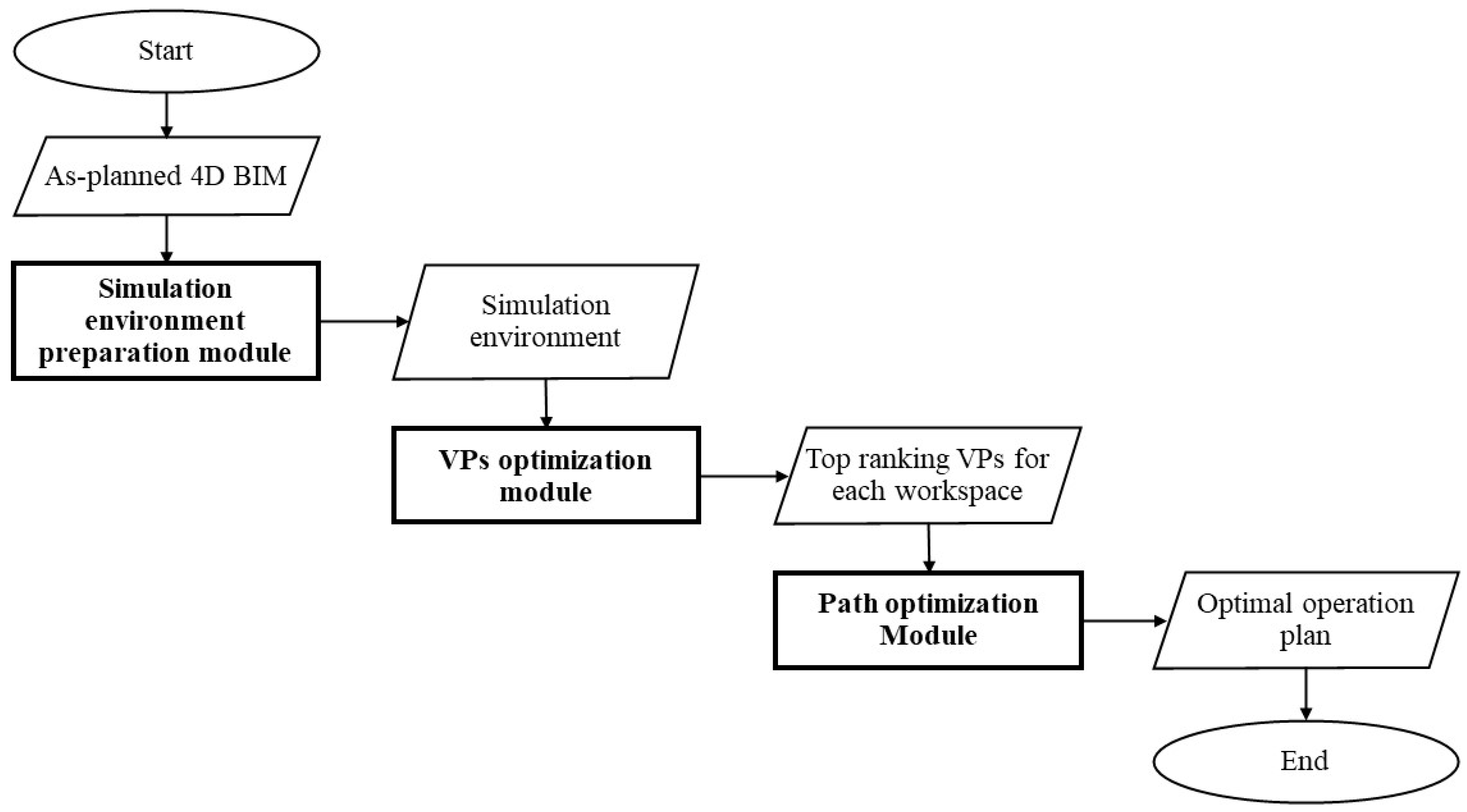
The proposed method considers the abovementioned requirements and optimizes the path of a CE-UAV that will hover at the top-ranking VPs to collect videos about construction activities of workers and equipment in different workspaces based on a micro-schedule. The proposed method consists of three modules, as shown in Figure 1: (1) preparation of the simulation platform; (2) VPs-optimization module; and (3) path-optimization module. These modules will be detailed in the subsequent sections.
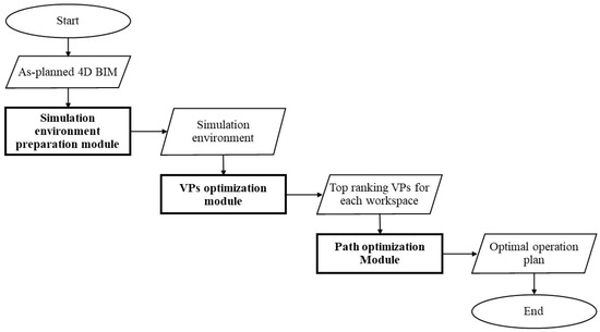
Figure 1.
Overview of proposed method.
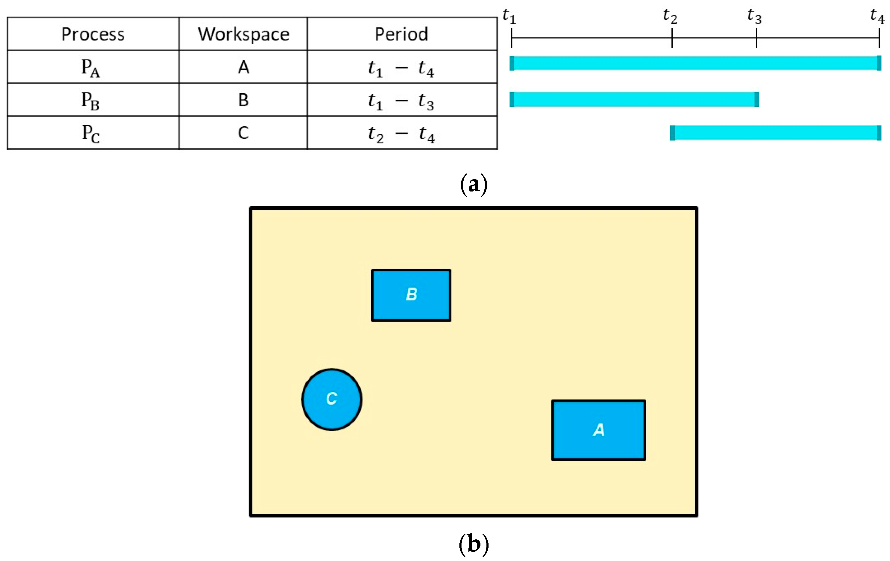
An example of a micro-schedule and the corresponding workspaces in the simulation environment are shown in Figure 2a and Figure 2b, respectively. In this example, three workspaces (i.e., A, B, and C) are identified from the as-planned 4D simulation of the project. A is the workspace for process PA, which is active during ; B is the workspace for PB during –; and C is the workspace for PC during –. The search space for each workspace is defined based on the solution variables, as will be explained in Section 3.2. Then, cubic cells are generated within the workspaces to prepare the simulation environment to calculate the camera coverage of the workspaces. Importance values (IVs) are assigned to the cells, considering the location (i.e., whether the cell is near the constructed objects) and the importance level of the associated task. In the VPs-optimization module, considering the workspaces and search spaces in each period, the top-ranking VPs, which are those in which the hovering camera has good coverage of the workspace while minimizing the distance to the workspace, are selected using a MOGA. In the path-optimization module, the Generalized Traveling Salesman Problem (GTSP) is solved by adapting a random-key GA to find the minimum-duration path that will allow the CE-UAV to collect videos from one of the top-ranking VPs in each workspace in a cyclic manner. The GTSP is an NP-hard problem and a variation of TSP, which aims to find the optimal Hamiltonian tour passing through one node from each cluster of nodes.
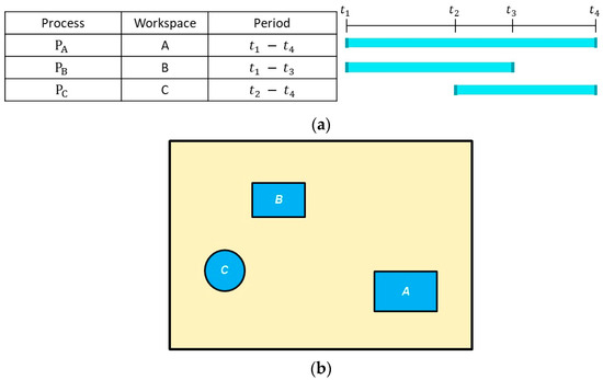
Figure 2.
Micro-schedule and corresponding workspaces. (a) Example of micro-schedule; (b) Corresponding workspaces.
Figure 3 shows the UAV optimal cycle paths in different periods for the above example. During , workspaces A and B are active. Multiple top-ranking VPs are identified in their corresponding search spaces (e.g., for workspace A, for workspace B). refers to the hovering time at point m. refers to the travel duration between point m and point n. Then, using the GA to solve the GTSP, and are selected as the top-ranking VPs to generate the path with the minimum travel duration. For the periods and , similar steps are followed to select the top-ranking VPs and to generate the optimal cycle paths. The cycle-path duration is determined by considering the desired data-capturing frequency (i.e., the expected number of cycles) and the maximum operation duration according to the UAV battery and payloads. Lastly, the hovering duration at each VP in one cycle is calculated, considering the importance level of the process.
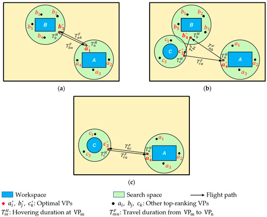
Figure 3.
UAV optimal cycle paths in different periods. (a) Period t1–t2; (b) Period t2–t3; (c) Period t3–t4.
3.2. Simulation-Environment-Preparation Module
Figure 4 shows the steps for preparing the simulation environment. In this module, the workspaces are identified from a detailed 4D simulation [49]. The hierarchy of a construction project used in this study is mainly adapted from [50], wherein five levels are identified: project, activity, construction operation, construction process, and work task. In practice, the project schedule is based on work packages representing activities and operations, which will take weeks or days. In this study, a micro-schedule is considered for workspace planning based on a sequence of processes, which will take hours or minutes. A CE-UAV can be used to capture videos of the activities of workers and equipment according to the micro-schedule, which will be used to extract detailed information about atomic activities.
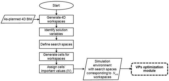
Figure 4.
Simulation-environment-preparation module.
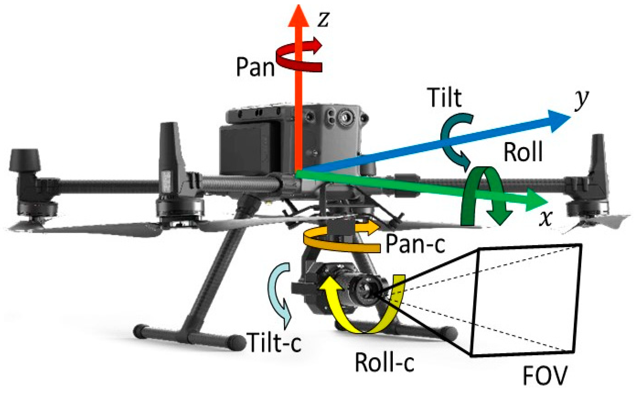
Then, the solution variables for the VPs-optimization module are identified. As shown in Figure 5, a CE-UAV has ten DoFs, six of which are related to the UAV’s pose (i.e., , ,, pan, tilt, and roll) and the other four of which control the mounted camera (pan-c, tilt-c, roll-c, and FOV). Incorporating the roll angle during image capture can increase the complexity and computational cost of CV processing. Therefore, in the proposed method, the sum of the rolls of the UAV and the camera is assumed to be zero. In addition, to simplify the variables in the optimization problem, the tilt angle of the UAV is assumed to be 0°, and the pan angle of the camera is assumed to be 0° to avoid occlusion by the legs of the UAV.
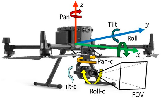
Figure 5.
Degrees of freedom of UAV and camera.
Moreover, the FOV of the camera is fixed to the default value (e.g., a diagonal FOV of 94°). Consequently, only the position of the UAV (, ,), the pan angle of the UAV (φ), and the tilt angle of the camera (θ) will be considered in the optimization.
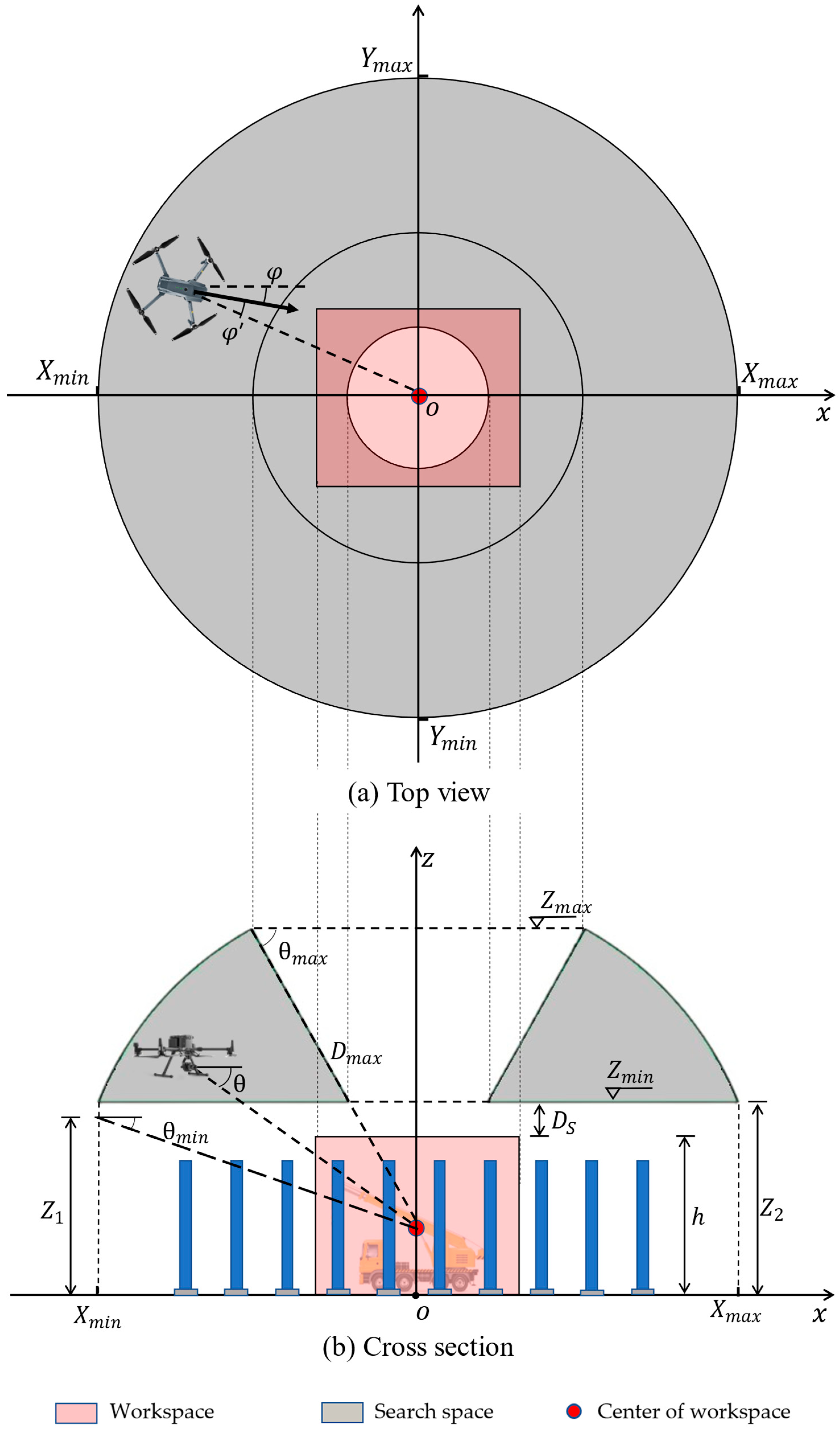
Figure 6a and Figure 6b show the top view and cross-section of the search space, respectively. Figure 6 also shows the solution variables (, ,, φ, and θ). In order to ensure good coverage of the workspace and capture the most informative scenes, the camera focus should be near the center of the workspace, where most of the construction activities are expected to happen. Instead of the pan angle () in the world coordinate system, the deviation () from the vector connecting the camera and the center of the workspace is used in the optimization, as shown in Figure 6a. The range for φ’ is set according to Equation (1), considering the trade-off between a larger search range and a faster optimization process.
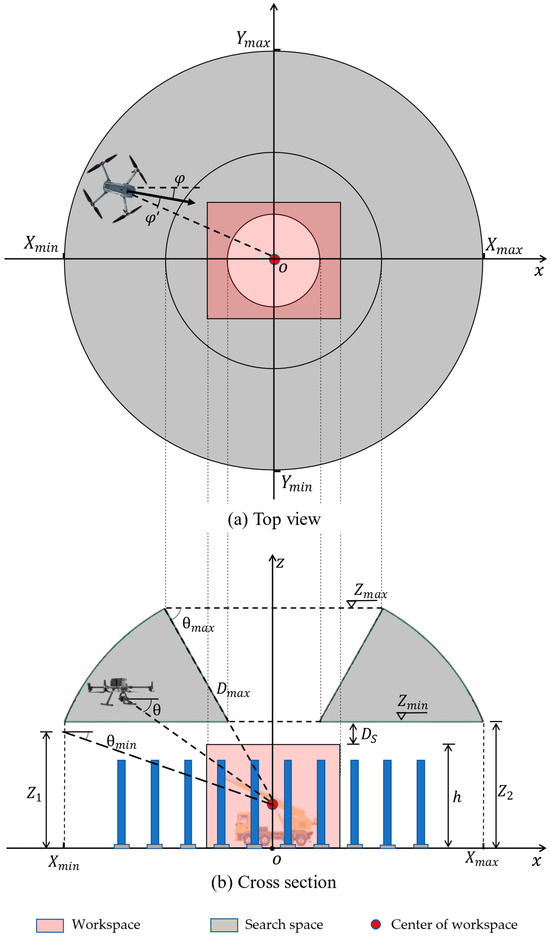
Figure 6.
Solution variables and the definition of the search space.
In addition, it is essential to maintain a tilt angle of the camera () that can clearly show the pose of workers and equipment according to Equation (2), as follows:
To define the range of (, ,), an assumption is made that and are set in a way that the focus of the camera is on the center of the workspace, as mentioned above. It is necessary to emphasize that this assumption applies only to the definition of the search space. As shown in Figure 6, for each workspace, the search space can be generated by considering the requirements explained in the previous section. The main constraints of the search space are the maximum distance () between the camera and the center of the workspace, the safe operation distance (), and the tilt angle range of the camera, subject to Equations (2)–(4). is the distance between the camera and the center of the workspace, which should be smaller than to avoid far-object detection with low resolution. To capture videos with an acceptable tilt angle, a limit is imposed on by considering and according to Equation (5), where is the height of the workspace. On the other hand, as shown in Equation (6), the value of is determined as the larger of two values: the minimum height (), as determined by according to Equation (7), and the sum of the workspace height and the safe operation distance, determined according to Equation (8). For instance, in the example depicted in Figure 6, is smaller than , resulting in being equal to . As a result of the above constraints, the search space is shown in the grey area in Figure 6.
The next step in preparing the simulation environment is generating cubic cells within the workspaces to calculate the camera coverage of workspaces. A trade-off is necessary between the accuracy of the coverage calculation and the computation time when defining the size of cells. Then, importance values () are calculated for these cells according to Equation (9), where is the base importance value of the cell, which is assigned according to the area in which the cell is located within the workspace. Specifically, the cells near the constructed objects are assigned higher values of . represents the weight assigned to the corresponding work process in the workspace, which indicates the complexity level of the associated processes. The weight of a workspace should be defined based on the project manager’s knowledge.
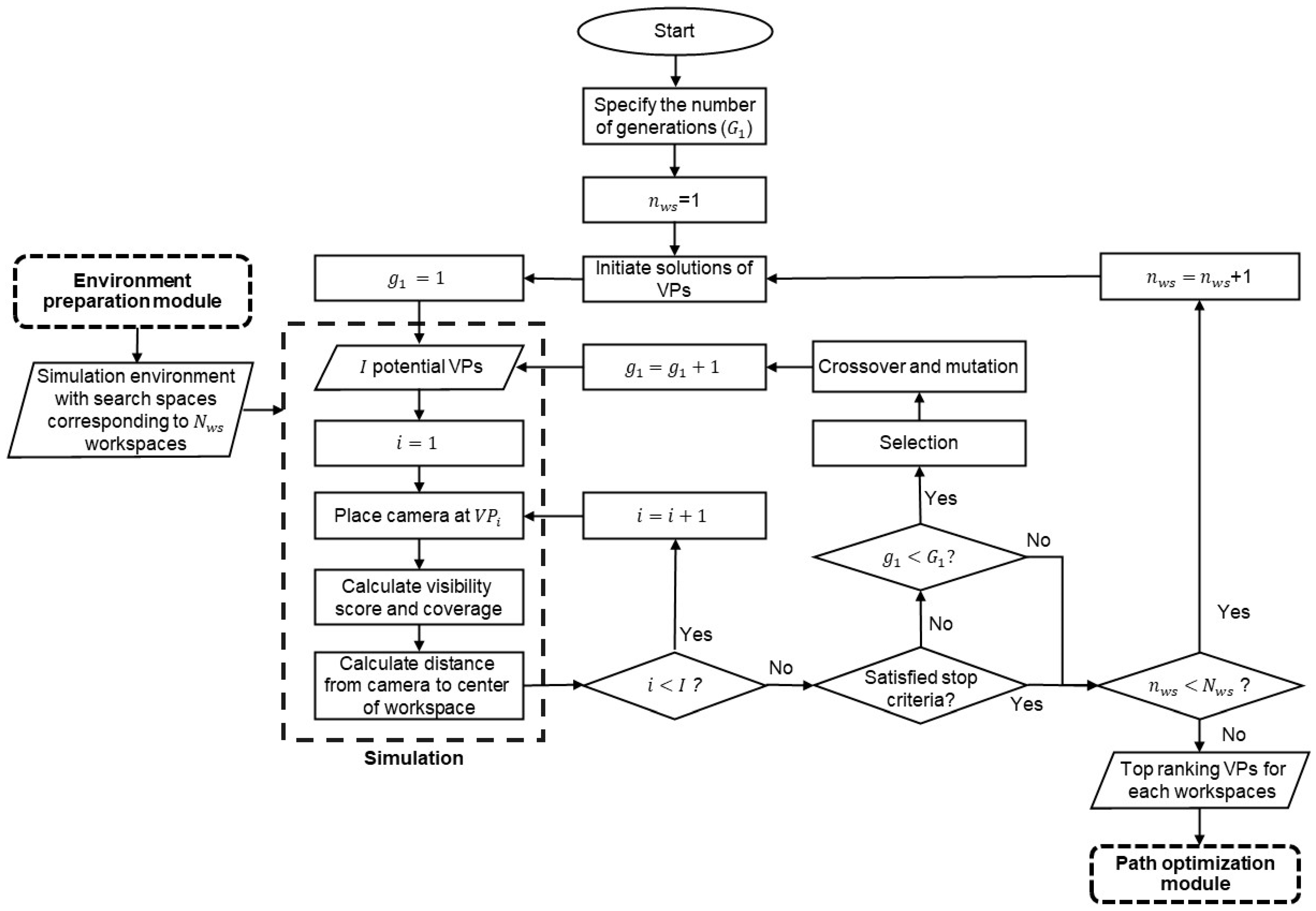
3.3. VPs-Optimization Module
Figure 7 shows the VPs-optimization process. The optimization of VPs is based on the camera’s visual coverage of the corresponding workspace and the distance from the camera to the center of the workspace, which are calculated in the simulation environment.

Figure 7.
VPs optimization module.
In this module, NSGA-II is adapted to identify the top-ranking VPs for each of the generated workspaces. NSGA-II was selected because of its remarkable computational efficiency in searching near-optimal solutions and its robust capability in managing uncertainty when compared with other metaheuristics algorithms (e.g., other GAs, Ant Colony Optimization (ACO), Particle Swarm Optimization (PSO)) for solving multiple-objective optimization problems [51]. Furthermore, NSGA-II’s simplicity and interpretability facilitate easy modification and enhancement, making it well-suited for addressing complex optimization problems [52], especially when additional conditions will be introduced to the simulation problem in the future.
It should be mentioned that some MOGA variants mentioned in Table 1 and Table 2 are not suitable for this purpose. Specifically, the Semantic-Cost GA [31] uses an inefficient selection operator, which selects solutions based on the probability derived from the fitness value. PMGA [5] and VL-MOGA [10] are specialized in other optimization aspects: PMGA performs multi-objective optimization in parallel across different scenarios to find the optimal VP for a fixed camera, considering various construction scenarios and stages. VL-MOGA optimizes a sequence of sampled VPs to improve the video-capturing plan for constructed buildings. However, neither of these methods can meet the requirements (as explained in Section 3.1) for identifying the top-ranking hovering VPs to capture videos of construction activities in a specific period according to the micro-schedule.
In each generation, a number of VPs are randomly generated within the search space. Then, the virtual CE-UAV is placed at each VP to calculate the visual coverage of the workspace through simulation. This simulation process can be illustrated using Equations (10) and (11). For the camera at , the set of visible cells is found using Equation (10), where is a visible cell, is the total number of visible cells when the camera is placed at , is a ray-tracing function that generates a collision-free ray between and the camera at , and is the field of view of the camera at . Based on the set of visible cells, the module then calculates the visibility score (), which is the summation of the IVs of visible cells according to Equation (11), where is a function that retrieves the IV of a cell.
The first objective function of the optimization maximizes the camera’s visual coverage () according to Equation (12), which is the visibility score divided by the sum of the IVs of the cells in the workspace. The second objective function minimizes the distance () from the to the center of the workspace, as shown in Equation (13), where is the position vector of the center of the workspace and is the position vector of . Using MOGA enables the identification of solutions (i.e., VPs) in the Pareto front that optimize the two objective functions. However, it is important to note that some of these solutions compromise visibility to minimize the distance to the workspace, such that the FOV does not cover the entire workspace. To avoid this issue, a constraint is imposed according to Equation (14), stipulating that the camera’s FOV at must encompass the entirety of the workspace, where denotes the generation of a ray originating from any cell within the workspace () towards the , regardless of occlusion. The multi-objective problem is constrained by Equations (1)–(4) and Equation (14).
The solution is subject to Equations (1)–(4)
Through the optimization, for each workspace, multiple top-ranking VPs will be identified. These VPs will then be ranked according to the fitness value, which should consider both objective functions. Therefore, normalization is applied to convert the distance used in Equation (13) into a percentage. Furthermore, since the other objective function is to maximize the coverage, Equation (15) is used to calculate the normalized distance () while transferring the objective function from a minimization to a maximization function. This is done by considering the distance from to the outer boundary of the search space along the vector from the center point of the workspace divided by the distance from the closest possible VP to the outer boundary. The fitness value is calculated using Equation (16), with weights and assigned to the visual coverage and normalized distance, respectively. The sum of the two weights should be 1, with a greater weight attributed to the visual coverage, reflecting its higher significance over a shorter distance. Finally, the ranked VPs are passed to the third module for path optimization.
3.4. Path-Optimization Module
Figure 8 shows the process of path optimization with the top-ranking VPs identified from the VPs-optimization module. This module solves the GTSP for the selection of the path with the shortest travel duration to collect videos from one of the top-ranking VPs for each workspace. For simplification, a simple UAV kinematic model is used without considering acceleration or turning constraints. It is considered that the CE-UAV will take off from the base station and travel to the first VP to start the monitoring for multiple cycle paths. After the last cycle is finished, the CE-UAV will return to the base station. The total duration of one cycle path is equal to the total flight time between the VPs () and the total hovering time at each of them as shown in Equation (17).
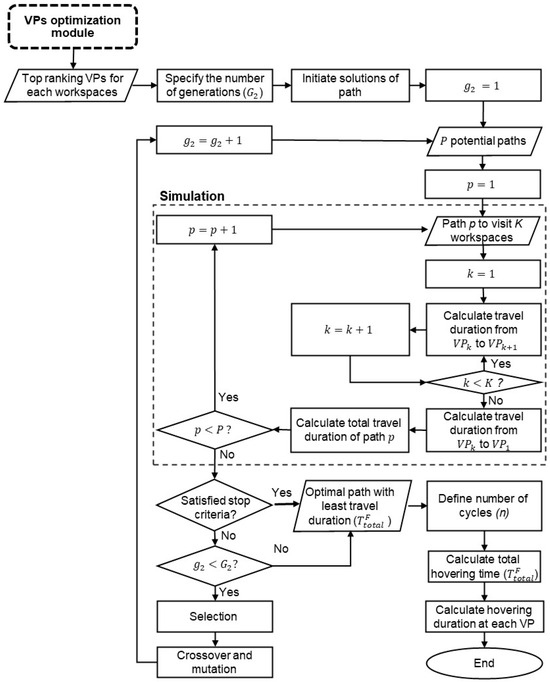
Figure 8.
Path-optimization module.
Assuming that the maximum operation time of the fully charged battery is , then the sum of , , and should be equal to the adjusted maximum operation time according to Equation (18), as follows:
where is a safety factor, n is the number of cycles, is the time needed for taking off and traveling from the base station to the first VP, and is the time needed to return to the base station. The proposed method aims to find the optimal path of one cycle by minimizing according to Equation (19). Then, the number of cycles n, the hovering time at each VP, and the first VP on the path connecting to the base station will be considered to generate the flight plan.
To find the optimal cycle path with the minimum , two variables are identified as necessary in this optimization problem: the ID of the VP to be selected in each workspace and the sequence in which the selected VPs are visited. The random-key GA [53] is adapted to solve this GTSP. The selection of this GA over alternative optimization techniques (e.g., PSO, ACO) is substantiated by its ability to find near-optimal solutions with short convergence time. In addition, while compared with other studies that applied simple GA for solving GTSP (e.g., [40] as shown in Table 2), the random-key GA is more robust regarding scalability and global search capability due to its lightweight encoding plan.
In this GA, the number of genes in the chromosome is determined based on the number of active workspaces that will be visited during a given period. For example, during t2–t3 in Figure 3b, the number of genes is three because there are three workspaces. The genes in the chromosome are in the order of the workspaces. A random float number between zero and the number of top-ranking VPs of the workspace is assigned to the kth gene. For decoding, each gene in the chromosome is divided into two components: an integer part and a fractional part. The integer part represents the index of the VP to be selected from the corresponding list of top-ranking VPs in workspace , where 0 denotes the first VP. Meanwhile, the fractional part corresponds to a random key. By sorting these random keys in ascending order, the sequence of workspaces to be visited can be obtained. For example, Table 3 shows an example of decoding a chromosome {3.83, 3.25, 1.77} for the case in Figure 3b. In workspace A, the integer part corresponds to 3, indicating the selection of the fourth VP in the list (). The same decoding process is applied to workspaces B and C to select the VPs to be visited. After the VPs have been sorted by their random keys in ascending order, the resulting sequence for visiting is ––.
Table 3.
Example of decoding a chromosome.
To complete the path to visit each VP generated by the GA, the first step entails identifying potential collisions between two consecutive VPs. If there is no obstacle on the path between them, a direct trajectory is generated. When the flight duration along this trajectory is computed, it should be noted that the UAV’s velocity constraints change when it moves vertically or horizontally. For example, in the case of DJI Matrice 100, the UAV ascends at a maximum speed of 5 m/s, descends at a maximum speed of 4 m/s, and reaches a maximum speed of 17 m/s when moving horizontally in GPS mode [54]. To address this, a weighted approach is employed to calculate the UAV’s velocity on the direct trajectory from one VP to another according to Equation (20), where is the maximum horizontal velocity, is the maximum vertical velocity in the corresponding move direction, and and are the horizontal distance and vertical distance between the two VPs, respectively.
On the other hand, if a potential collision is detected, the A* search algorithm is used to find the collision-free UAV trajectory between two consecutive VPs. The A* algorithm was selected due to its robust overall performance in efficiently and accurately finding collision-free optimal paths within various 3D maps [55]. Additionally, its simplicity in application within the simulation environment of this study was a significant factor. The 3D space is discretized into a 3D cubic grid. The A* algorithm searches the trajectory based on the time needed for the UAV to travel from the given starting node to the node while avoiding collision and the estimated remaining time for the UAV to travel from to the goal position GP. can be calculated according to Equation (21), where is the travel time needed for the UAV to travel from to . Meanwhile, is calculated according to Equation (22), where is the heuristic function used to estimate the travel time from to the GP regardless of collision. The sum of these two times will be used to determine whether the trajectory should go through node , according to Equation (23).
with the optimal cycle path, it is possible to select the first VP on the path that is closest to the base station and to calculate and . The next step is to calculate the hovering duration at each VP and the number of cycles that the CE-UAV can complete in one flight with a fully charged battery. Based on Equations (17) and (18), the equation for determining can be derived as shown in Equation (24). To determine , a trade-off is needed between frequent monitoring (i.e., the value of n) and longer hovering duration in each cycle. In other words, a shorter cycle-path time with more cycles in one operation results in less time spent hovering at each VP and relatively longer travel time between VPs. On the other hand, a longer cycle-path time may lead to missing some events at certain VPs because the CE-UAV is hovering at other VPs and the frequency of visits to all VPs is lower.
The distribution of at different VPs should prioritize the coverage achievable at each VP and the importance level of the task. Therefore, the hovering time at each is calculated based on the coverage ) of the corresponding workspace and the importance level of the task, according to Equation (25), where is the assigned weight for workspace , as explained in Section 3.2.
4. Implementation and Case Study
In this section, the implementation of the proposed method is introduced and a case study is conducted to validate the performance of the proposed method.
4.1. Implementation
A prototype system was developed using the Unity3D game engine (v.2022.3.27f1, San Francisco, CA, USA) [56] and Python programming language (v.3.10.12) [57]. The BIM model of the case-study project was imported into Unity3D to create a simulation platform for calculating visibility scores using the Raycast function to detect potential occlusion between the VPs and the generated cells of the workspace. NSGA-II was applied for the optimization of VPs using the open-source Pymoo library [58] (East Lansing, MI, USA) in Python. In addition, the path-optimization module customized the random-key GA based on Pymoo to solve the GTSP. A collider was generated in the game engine based on the positions of the two VPs in the path to detect potential collision risks while considering the safe operation distance. If any potential collision was detected, A* 3D pathfinding function [59] in Unity3D was used to determine the optimal path between them. The communication between Unity3D (client) and Python (server) was established using the Transmission Control Protocol/Internet Protocol (TCP/IP). The prototype system was tested on a computer with Intel i7-6800k CPU (Santa Clara, CA, USA), 64 GB of random-access memory (RAM) and two Nvidia GTX 1070 GPUs (Santa Clara, CA, USA).
4.2. Case Study
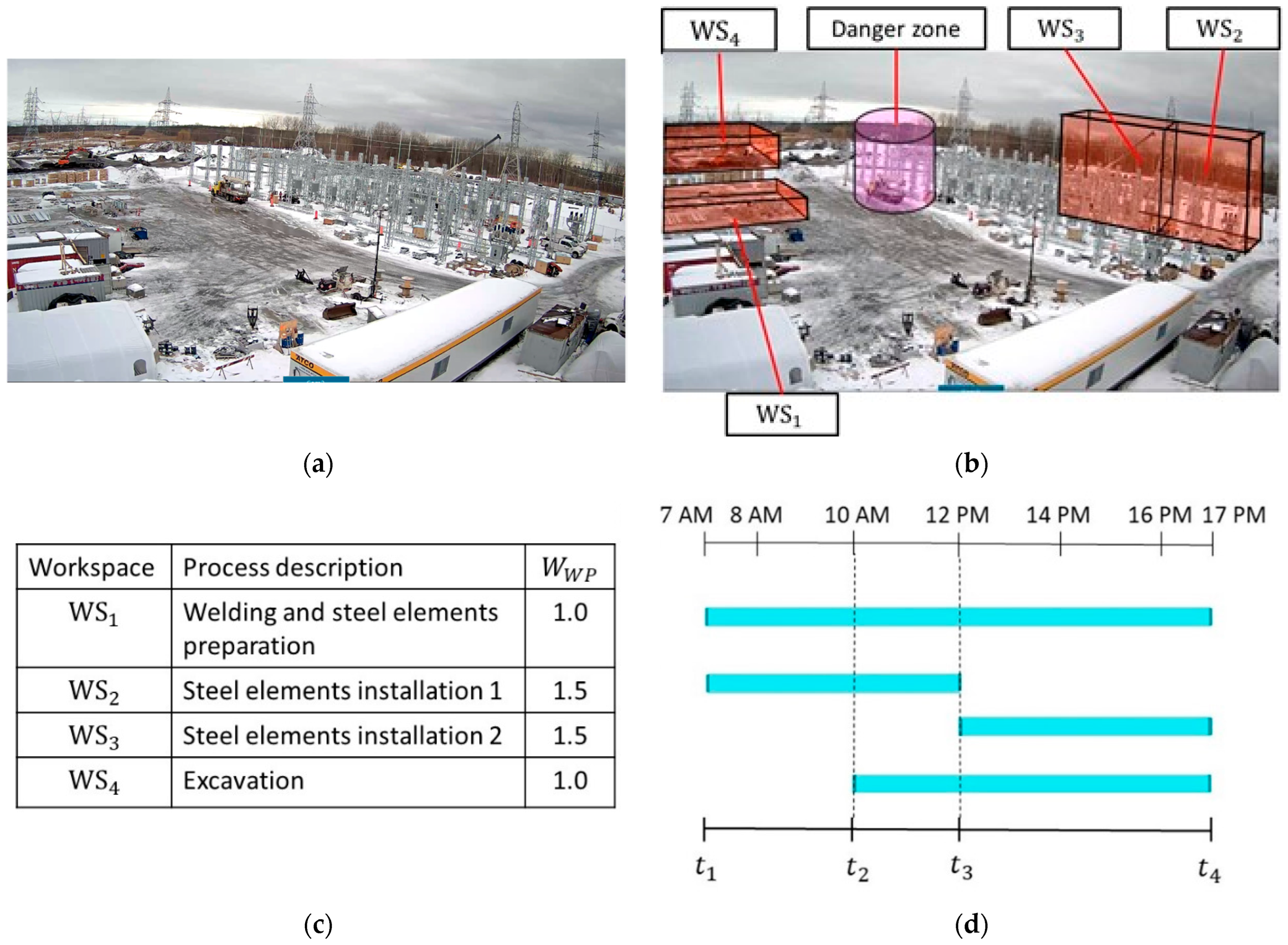
A case study was conducted to validate the applicability of the proposed method and the developed prototype system. The case study was developed based on activities during one day on the construction site of an electric substation. Figure 9 shows the workspaces on the construction site and the schedule of the corresponding processes. The process of welding and steel-element preparation were carried out in WS1. The processes of steel elements installation were split into two separate workspaces due to the crane’s relocation. The process of steel-element installation 1 was carried out in WS2 during –. During –, the crane was relocated to WS3 to finish the process of steel-element installation 2. In addition, one excavator was doing earthwork in WS4 during –. Near the middle of the construction site, a cylindric volume with a radius of 10 m and a height of 20 m was reserved for an idling crane as a danger zone for the UAV. Due to the higher level of complexity associated with the processes of steel-element installation compared to the other two processes, a higher weight () of 1.5 was assigned to WS2 and WS3, given that the of the regular processes (in WS1 and WS4) had a value of 1.
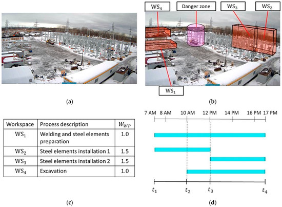
Figure 9.
(a) Construction site; (b) workspaces and danger zone; (c) workspace details; and (d) micro-schedule.
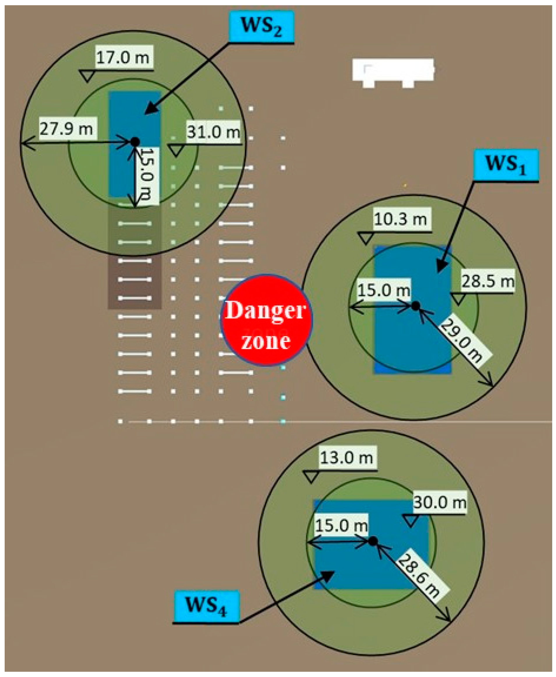
By combining the 3D BIM and the schedule, 4D simulation was generated and used as the input for generating the workspace model in Unity3D. The safe operation distance () was set to 5 m, and the maximum distance () was set to 30 m. The search space was then generated according to the steps explained in Section 3.2. Table 4 lists the location of each workspace and the range of attribute values of the corresponding search space. As an example, Figure 10 shows the top view of the search spaces for the three workspaces during –. Then, cells were generated with the dimensions 1 m × 1 m × 1 m, and the base importance value of each cell was set to 1 for simplification.
Table 4.
Search-space dimensions.
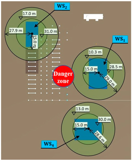
Figure 10.
Search spaces for period t2–t3.
The UAV considered in the case study is a DJI Matrice 100 (Shenzhen, China) equipped with a DJI TB48D battery, which can ascend at a maximum speed of 5 m/s, descend at a maximum speed of 4 m/s, and reach a top speed of 17 m/s in GPS mode. Therefore, the time the UAV takes to travel between two points at different heights will vary, as explained in Section 3.4. The only payload carried by the UAV is assumed to be the DJI Zenmuse X3 4K camera (Shenzhen, China), which has a diagonal FOV of 94° (vertical FOV of about 62° and horizontal FOV of about 84°). This payload allows for an approximate flight time of 24 min [40]. The safety factor for the maximum operation duration was set to 0.9.
In the NSGA-II, which was used to identify the top-ranking VPs, the number of generations was set at 70, with a population size of 300. The algorithm employs a two-point crossover with a probability of 80% and a polynomial mutation with a mutation probability that can be calculated according to Equation (26) [60]. is determined by the number of variables. In this case study, with five variables in the VPs optimization (), was 20%. In addition, the distribution index for mutation () was set to 30, noting that a lower leads to a wider spread of the mutated value. Moreover, to rank the VPs generated by the VPs-optimization module, and (Equation (16)) were set to 0.8 and 0.2, respectively.
The GA for GTSP used 100 generations but a smaller population size of 200 due to the smaller search space. It employed a single-point crossover with a probability of 80% and random mutation with a probability of 5%.
4.3. Pilot Test for Evaluating the VPs-Optimization Module
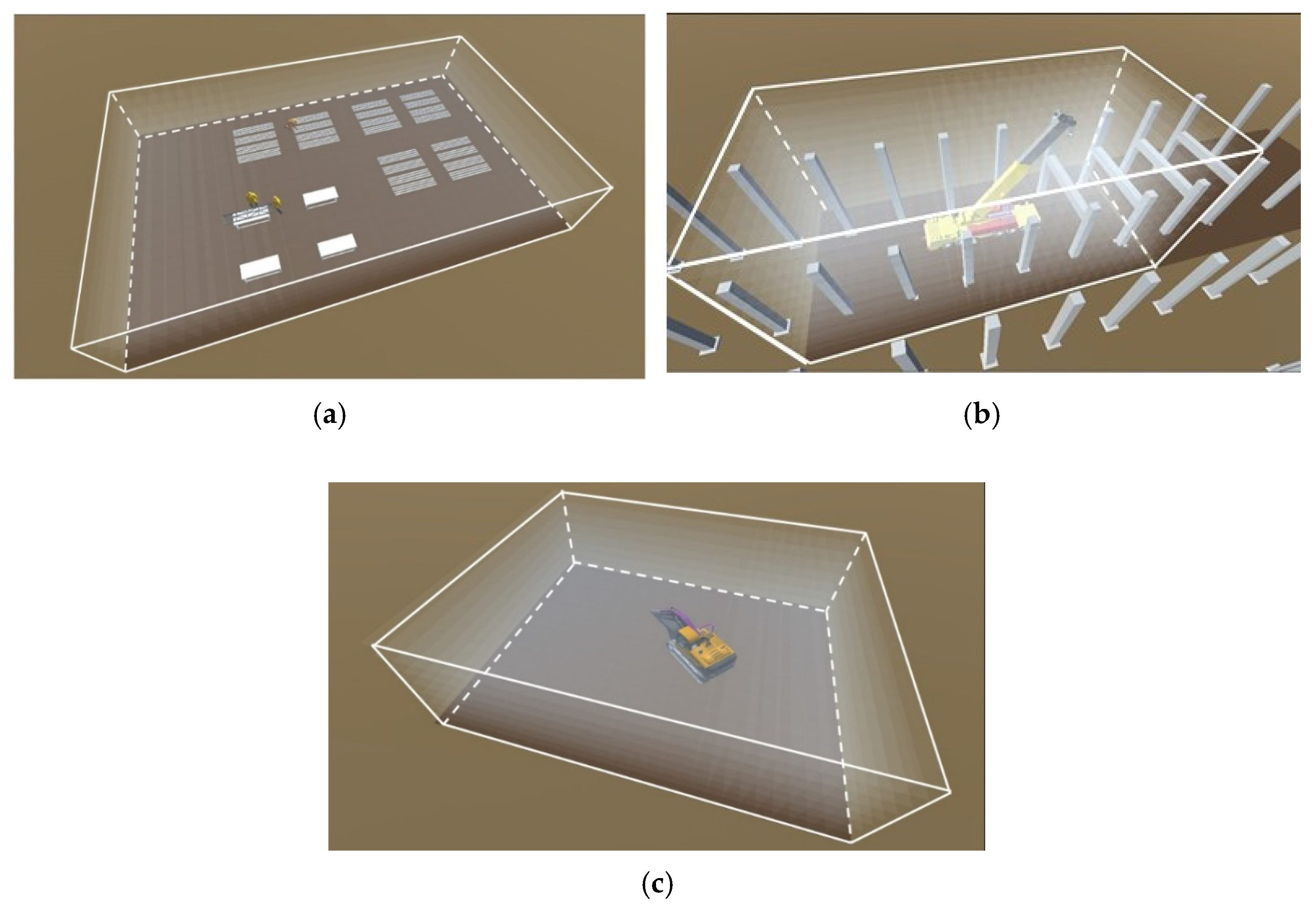
A pilot test was conducted to evaluate the performance of the VPs optimization module under various hypothetical conditions with artificial walls, ranging from highly confined workspaces to open environments. Three distinct scenarios were generated, as shown in Figure 11, focusing on WS2. In the first scenario (Figure 11a), the workspace was positioned in an open space with minimal nearby structures serving as potential obstacles. Figure 11b depicts the second scenario, where the workspace was surrounded by 12-m-high walls acting as primary obstacles. Gaps were intentionally left between the walls to enable the CE-UAV to observe the workspace from the outside. The third scenario, as illustrated in Figure 11c, presented an extreme condition in which the workspace was surrounded by tall walls 20 m in height. The views of cameras form the optimal VP in each scenario are also shown correspondingly. In this figure, the cells that are completely or partially invisible to the camera are highlighted in red. It is important to note that some invisible cells may still appear within the cameras’ views because these cells are only partially occluded.

Figure 11.
Pilot test and the optimal VP in each scenario.
The VPs-optimization module identified multiple top-ranking VPs for each scenario, as listed in Table 5. The optimal VPs with the highest fitness value in each scenario are marked in the table. In general, the optimization module successfully identified VPs that provided optimal coverage with a short distance to the workspace in different scenarios. Even when faced with artificial obstacles, the module could still find the VPs that covered over 95% of the workspace. However, extreme conditions can introduce constraints on the positions of the identified VPs, leading to increased distances between the VPs and the workspace. In particular, the taller walls in Scenario 3 resulted in greater distances between the VPs and the workspace.
Table 5.
Optimized VPs in different scenarios.
4.4. Results of the Case Study
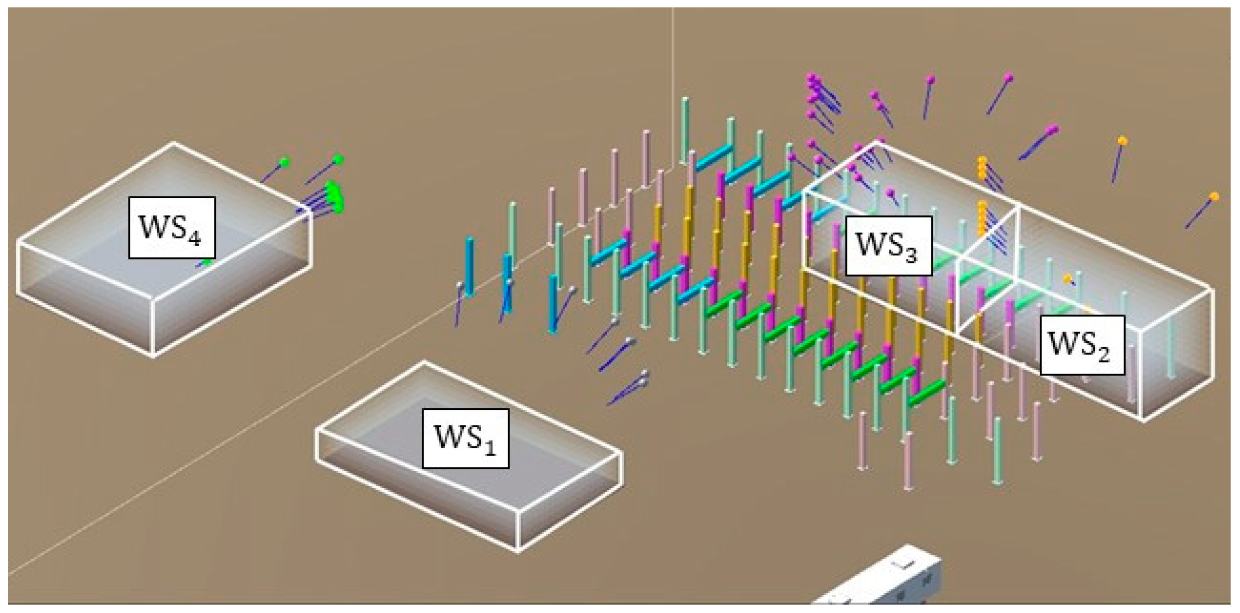
In the VPs-optimization module, multiple top-ranking VPs for each workspace can be identified, as shown in Figure 12. To save processing time in the path-optimization module, only the best three VPs are retained. As a result, Table 6 lists the VPs that were passed to the path-optimization module, along with their position, orientation, coverage, distance to the center of the workspace, and fitness value. For WS2 and WS3, the overall coverage at each of the top-ranking VPs exceeded 90%. For WS1 and WS4, where there were no obstacles, the visual coverage was 100%. These results demonstrate the effectiveness of the selected VPs in providing high coverage of the workspaces while minimizing the distance to the workspace.
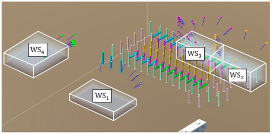
Figure 12.
Top-ranking VPs for each workspace.
Table 6.
Selected VPs.
With the top-ranking VPs, the path-optimization module generated the optimized path for each time period. The optimal paths and their corresponding durations are shown in Table 7. During –, VP1-VP4-VP1 was the optimal path. VP1, which was the closest VP to the UAV base station, near the construction-site office, was selected as the first destination. As a result of the differing ascent and descent speeds, the take-off time from the base station to VP1 was 4.15 s and the landing time was 4.66 s. The total flight duration between the VPs within one cycle was 5.93 s. In the period –, the optimal path was VP3-VP12-VP4-VP3, with VP3 as the first destination. The take-off time was 5.04 s, and the landing time was 5.58 s. The total flight duration between the VPs in one cycle was 10.97 s. During –, the optimal path was VP3-VP12-VP8-VP3, where VP3 remained the first destination. The total flight duration between VPs within one cycle was 9.37 s.
Table 7.
Optimal paths and path durations in different periods.
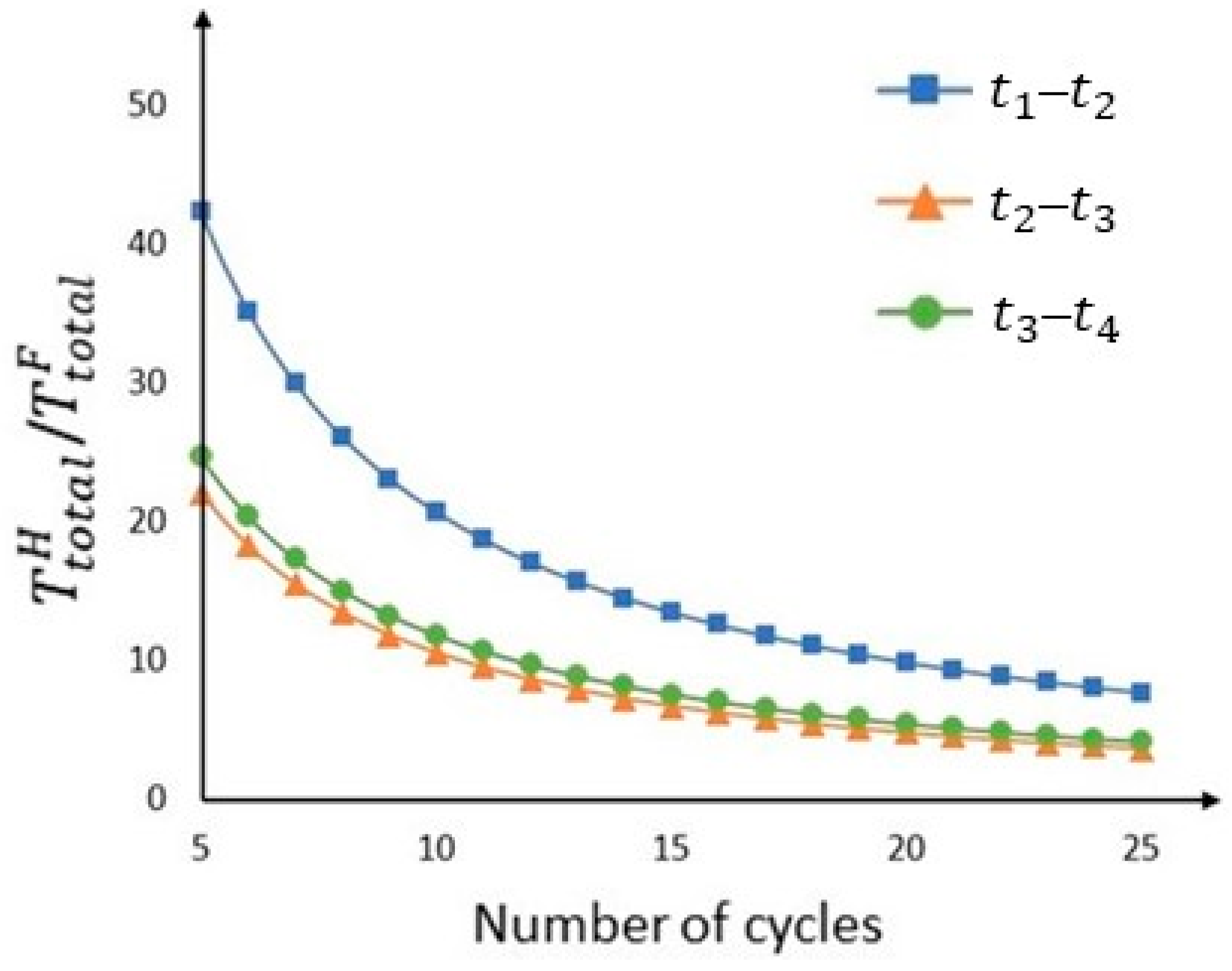
Then, the total hovering times were calculated according to Section 3.4. As mentioned in Section 4.2, the flight time was 24 min. With a safety factor of 0.9, the maximum operation duration was 1296 s. Designating more cycles within one operation led to more frequent visits by the VPs but shorter hovering times and relatively more time spent in transit. Figure 13 shows the relationship between the number of cycles and the ratio /. As explained in Section 3.4, there is a trade-off between and n. Therefore, in this case study, n was set to 11, resulting in a of less than 2 min for all durations, as shown in Table 7.

Figure 13.
Relationship between the number of cycles and the ratio /.
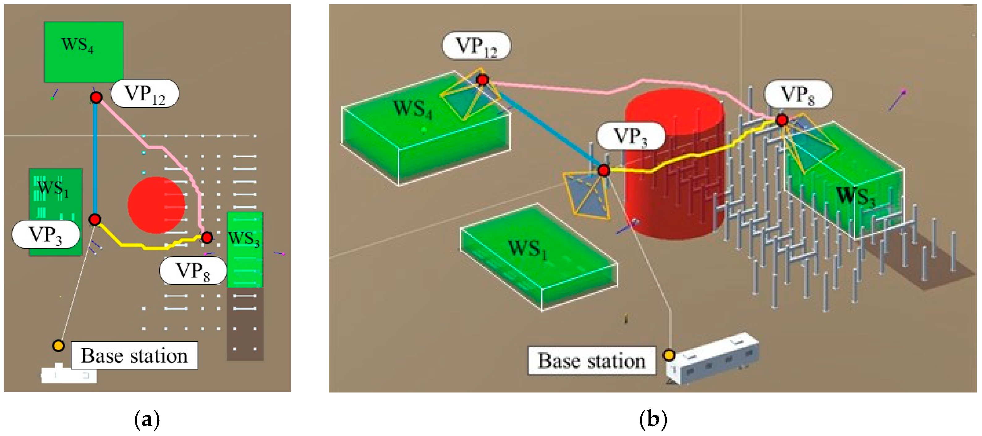
The distributions of the hovering times for each of the VPs were calculated according to Equation (25), as shown in Figure 14. Figure 15 shows the optimal path during –. Figure 16 shows the simulated views of the camera hovering at the three VPs for the optimal path.
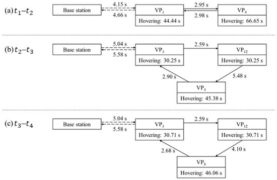
Figure 14.
Optimal paths in different periods. (a) Period –; (b) Period –; (c) Period –.
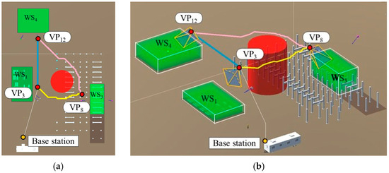
Figure 15.
Optimal path in the period t3–t4. (a) Top view; (b) 3D view.

Figure 16.
Simulated views of the camera hovering at optimal VPs in the period t3–t4. (a) View of the workshop (WS1) from VP3; (b) view of the crane installing steel elements (WS3) from VP8; (c) view of excavation work (WS4) from VP12.
5. Conclusions and Future Work
In this paper, a method is proposed for optimizing the path of a CE-UAV to collect videos showing the construction activities of workers and equipment. The proposed method includes a simulation-based VPs optimization using a MOGA that identifies the top-ranking VPs for various workspaces. Subsequently, a GA algorithm is applied to minimize the travel duration by solving the GTSP based on the identified VPs, which generates an optimal path. As explained in Section 2.2, this method focuses on collecting videos with good visual coverage of dynamic construction activities, while previous studies focused on the scanning of the constructed objects. To evaluate the proposed method, a case study was conducted using a prototype system developed using the Unity3D game engine and Python. The results of the pilot test show that the VPs-optimization module can find the optimal VPs with excellent workspace coverage while minimizing the distance to the workspaces in different scenarios with different occlusions. In addition, the case-study results demonstrate that the method can effectively optimize the VPs for different workspaces and generate optimal paths with the shortest travel durations to collect videos of construction activities according to the micro-schedule.
The main contributions of this research are as follows: (1) developing a method to identify the top-ranking VPs of CE-UAVs to capture videos of construction activities based on a detailed 4D simulation; (2) developing a method for planning the optimal path of a CE-UAV to minimize travel time while avoiding collisions; and (3) developing a prototype system based on the proposed method that validated the feasibility and applicability in a simulated environment.
There are several limitations in this research: (1) the proposed method generates the optimal paths based on the information available in the 4D simulation without considering other potential unexpected temporary obstacles, such as equipment passing by; (2) the case study presented in this research is based on a medium-scale construction site situated in an open space, where the likelihood of occlusion is relatively low; (3) the optimized path has been validated only in a simulation environment. It is necessary to deploy path optimization on actual construction sites using autonomous UAVs to further verify the effectiveness of the proposed method; (4) the optimization and pathfinding algorithms were selected for their robustness in solving the specific problems described in Section 3.3 and Section 3.4. However, these algorithms may have limitations, particularly when additional conditions and constraints are introduced to the optimization problem; and (5) the continuous collection of video of construction activities is limited by the operation time of the UAV, which is relatively short due to the battery capacity.
When considering the application of the research, the abovementioned limitations have to be addressed in future work, as follows: (1) more efforts should be made in the future to apply real-time obstacle detection and avoidance; (2) a more comprehensive case study should be conducted to test the effectiveness of the proposed method in diverse construction environments, such as indoor environments with more potential occlusions; (3) further field tests should be conducted to deploy path optimization on real construction sites using autonomous UAVs, providing practical validation of the method beyond simulation environments; (4) future work should compare the selected optimization and pathfinding algorithms with their competent alternatives, aiming to refine the methodology regarding accuracy and efficiency; and (5) future research should explore new solutions to mitigate the challenge of the short operation time, such as utilizing multiple UAVs or tethered UAVs.
Author Contributions
Conceptualization, Y.H. and A.H.; Methodology, Y.H.; Writing—original draft, Y.H.; Writing—review & editing, A.H.; Supervision, A.H. All authors have read and agreed to the published version of the manuscript.
Funding
This research received no external funding.
Data Availability Statement
The raw data supporting the conclusions of this article will be made available by the authors on request.
Conflicts of Interest
The authors declare no conflict of interest.
References
- Alizadehsalehi, S.; Yitmen, I. The Impact of Field Data Capturing Technologies on Automated Construction Project Progress Monitoring. Procedia Eng. 2016, 161, 97–103. [Google Scholar] [CrossRef]
- Yang, J.; Park, M.-W.; Vela, P.A.; Golparvar-Fard, M. Construction Performance Monitoring via Still Images, Time-Lapse Photos, and Video Streams: Now, Tomorrow, and the Future. Adv. Eng. Inform. 2015, 29, 211–224. [Google Scholar] [CrossRef]
- Paneru, S.; Jeelani, I. Computer Vision Applications in Construction: Current State, Opportunities & Challenges. Autom. Constr. 2021, 132, 103940. [Google Scholar] [CrossRef]
- Xu, S.; Wang, J.; Shou, W.; Ngo, T.; Sadick, A.-M.; Wang, X. Computer Vision Techniques in Construction: A Critical Review. Arch. Comput. Methods Eng. 2021, 28, 3383–3397. [Google Scholar] [CrossRef]
- Chen, X.; Zhu, Y.; Chen, H.; Ouyang, Y.; Luo, X.; Wu, X. BIM-Based Optimization of Camera Placement for Indoor Construction Monitoring Considering the Construction Schedule. Autom. Constr. 2021, 130, 103825. [Google Scholar] [CrossRef]
- Tran, S.V.-T.; Nguyen, T.L.; Chi, H.-L.; Lee, D.; Park, C. Generative Planning for Construction Safety Surveillance Camera Installation in 4D BIM Environment. Autom. Constr. 2022, 134, 104103. [Google Scholar] [CrossRef]
- Asadi, K.; Kalkunte Suresh, A.; Ender, A.; Gotad, S.; Maniyar, S.; Anand, S.; Noghabaei, M.; Han, K.; Lobaton, E.; Wu, T. An Integrated UGV-UAV System for Construction Site Data Collection. Autom. Constr. 2020, 112, 103068. [Google Scholar] [CrossRef]
- Ham, Y.; Han, K.K.; Lin, J.J.; Golparvar-Fard, M. Visual Monitoring of Civil Infrastructure Systems via Camera-Equipped Unmanned Aerial Vehicles (UAVs): A Review of Related Works. Vis. Eng. 2016, 4, 1. [Google Scholar] [CrossRef]
- Jeelani, I.; Gheisari, M. Safety Challenges of UAV Integration in Construction: Conceptual Analysis and Future Research Roadmap. Saf. Sci. 2021, 144, 105473. [Google Scholar] [CrossRef]
- Ibrahim, A.; Golparvar-Fard, M.; El-Rayes, K. Multiobjective Optimization of Reality Capture Plans for Computer Vision–Driven Construction Monitoring with Camera-Equipped UAVs. J. Comput. Civ. Eng. 2022, 36, 04022018. [Google Scholar] [CrossRef]
- Ivić, S.; Crnković, B.; Grbčić, L.; Matleković, L. Multi-UAV Trajectory Planning for 3D Visual Inspection of Complex Structures. Autom. Constr. 2023, 147, 104709. [Google Scholar] [CrossRef]
- Zheng, X.; Wang, F.; Li, Z. A Multi-UAV Cooperative Route Planning Methodology for 3D Fine-Resolution Building Model Reconstruction. ISPRS J. Photogramm. Remote Sens. 2018, 146, 483–494. [Google Scholar] [CrossRef]
- Huang, Y.; Amin, H. Simulation-Based Optimization of Path Planning for Camera-Equipped UAV Considering Construction Activities. In Proceedings of the Creative Construction Conference 2023, Keszthely, Hungary, 20–23 June 2023. [Google Scholar]
- Yang, J.; Shi, Z.; Wu, Z. Vision-Based Action Recognition of Construction Workers Using Dense Trajectories. Adv. Eng. Inform. 2016, 30, 327–336. [Google Scholar] [CrossRef]
- Roh, S.; Aziz, Z.; Peña-Mora, F. An Object-Based 3D Walk-through Model for Interior Construction Progress Monitoring. Autom. Constr. 2011, 20, 66–75. [Google Scholar] [CrossRef]
- Kropp, C.; Koch, C.; König, M. Interior Construction State Recognition with 4D BIM Registered Image Sequences. Autom. Constr. 2018, 86, 11–32. [Google Scholar] [CrossRef]
- Rebolj, D.; Pučko, Z.; Babič, N.Č.; Bizjak, M.; Mongus, D. Point Cloud Quality Requirements for Scan-vs-BIM Based Automated Construction Progress Monitoring. Autom. Constr. 2017, 84, 323–334. [Google Scholar] [CrossRef]
- Son, H.; Bosché, F.; Kim, C. As-Built Data Acquisition and Its Use in Production Monitoring and Automated Layout of Civil Infrastructure: A Survey. Adv. Eng. Inform. 2015, 29, 172–183. [Google Scholar] [CrossRef]
- Chen, C.; Zhu, Z.; Hammad, A. Automated Excavators Activity Recognition and Productivity Analysis from Construction Site Surveillance Videos. Autom. Constr. 2020, 110, 103045. [Google Scholar] [CrossRef]
- Wang, Z.; Zhang, Q.; Yang, B.; Wu, T.; Lei, K.; Zhang, B.; Fang, T. Vision-Based Framework for Automatic Progress Monitoring of Precast Walls by Using Surveillance Videos during the Construction Phase. J. Comput. Civ. Eng. 2021, 35, 04020056. [Google Scholar] [CrossRef]
- Arif, F.; Khan, W.A. Smart Progress Monitoring Framework for Building Construction Elements Using Videography–MATLAB–BIM Integration. Int. J. Civ. Eng. 2021, 19, 717–732. [Google Scholar] [CrossRef]
- Soltani, M.M.; Zhu, Z.; Hammad, A. Framework for Location Data Fusion and Pose Estimation of Excavators Using Stereo Vision. J. Comput. Civ. Eng. 2018, 32, 04018045. [Google Scholar] [CrossRef]
- Bohn, J.S.; Teizer, J. Benefits and Barriers of Construction Project Monitoring Using High-Resolution Automated Cameras. J. Constr. Eng. Manag. 2010, 136, 632–640. [Google Scholar] [CrossRef]
- Fang, W.; Ding, L.; Luo, H.; Love, P.E.D. Falls from Heights: A Computer Vision-Based Approach for Safety Harness Detection. Autom. Constr. 2018, 91, 53–61. [Google Scholar] [CrossRef]
- Zhang, H.; Yan, X.; Li, H. Ergonomic Posture Recognition Using 3D View-Invariant Features from Single Ordinary Camera. Autom. Constr. 2018, 94, 1–10. [Google Scholar] [CrossRef]
- Bügler, M.; Borrmann, A.; Ogunmakin, G.; Vela, P.A.; Teizer, J. Fusion of Photogrammetry and Video Analysis for Productivity Assessment of Earthwork Processes. Comput.-Aided Civ. Infrastruct. Eng. 2017, 32, 107–123. [Google Scholar] [CrossRef]
- Luo, X.; Li, H.; Yang, X.; Yu, Y.; Cao, D. Capturing and Understanding Workers’ Activities in Far-Field Surveillance Videos with Deep Action Recognition and Bayesian Nonparametric Learning. Comput.-Aided Civ. Infrastruct. Eng. 2019, 34, 333–351. [Google Scholar] [CrossRef]
- Torabi, G.; Hammad, A.; Bouguila, N. Two-Dimensional and Three-Dimensional CNN-Based Simultaneous Detection and Activity Classification of Construction Workers. J. Comput. Civ. Eng. 2022, 36, 04022009. [Google Scholar] [CrossRef]
- Park, M.-W.; Elsafty, N.; Zhu, Z. Hardhat-Wearing Detection for Enhancing On-Site Safety of Construction Workers. J. Constr. Eng. Manag. 2015, 141, 04015024. [Google Scholar] [CrossRef]
- Albahri, A.H.; Hammad, A. Simulation-Based Optimization of Surveillance Camera Types, Number, and Placement in Buildings Using BIM. J. Comput. Civ. Eng. 2017, 31, 04017055. [Google Scholar] [CrossRef]
- Kim, J.; Ham, Y.; Chung, Y.; Chi, S. Systematic Camera Placement Framework for Operation-Level Visual Monitoring on Construction Jobsites. J. Constr. Eng. Manag. 2019, 145, 04019019. [Google Scholar] [CrossRef]
- Yang, X.; Li, H.; Huang, T.; Zhai, X.; Wang, F.; Wang, C. Computer-Aided Optimization of Surveillance Cameras Placement on Construction Sites. Comput.-Aided Civ. Infrastruct. Eng. 2018, 33, 1110–1126. [Google Scholar] [CrossRef]
- Zhang, Y.; Luo, H.; Skitmore, M.; Li, Q.; Zhong, B. Optimal Camera Placement for Monitoring Safety in Metro Station Construction Work. J. Constr. Eng. Manag. 2019, 145, 04018118. [Google Scholar] [CrossRef]
- Maboudi, M.; Homaei, M.; Song, S.; Malihi, S.; Saadatseresht, M.; Gerke, M. A Review on Viewpoints and Path Planning for UAV-Based 3-D Reconstruction. IEEE J. Sel. Top. Appl. Earth Obs. Remote Sens. 2023, 16, 5026–5048. [Google Scholar] [CrossRef]
- Freimuth, H.; König, M. Planning and Executing Construction Inspections with Unmanned Aerial Vehicles. Autom. Constr. 2018, 96, 540–553. [Google Scholar] [CrossRef]
- Li, F.; Zlatanova, S.; Koopman, M.; Bai, X.; Diakité, A. Universal Path Planning for an Indoor Drone. Autom. Constr. 2018, 95, 275–283. [Google Scholar] [CrossRef]
- Bircher, A.; Kamel, M.; Alexis, K.; Burri, M.; Oettershagen, P.; Omari, S.; Mantel, T.; Siegwart, R. Three-Dimensional Coverage Path Planning via Viewpoint Resampling and Tour Optimization for Aerial Robots. Auton. Robots 2016, 40, 1059–1078. [Google Scholar] [CrossRef]
- Phung, M.D.; Quach, C.H.; Dinh, T.H.; Ha, Q. Enhanced Discrete Particle Swarm Optimization Path Planning for UAV Vision-Based Surface Inspection. Autom. Constr. 2017, 81, 25–33. [Google Scholar] [CrossRef]
- Huang, X.; Liu, Y.; Huang, L.; Stikbakke, S.; Onstein, E. BIM-Supported Drone Path Planning for Building Exterior Surface Inspection. Comput. Ind. 2023, 153, 104019. [Google Scholar] [CrossRef]
- Bolourian, N.; Hammad, A. LiDAR-Equipped UAV Path Planning Considering Potential Locations of Defects for Bridge Inspection. Autom. Constr. 2020, 117, 103250. [Google Scholar] [CrossRef]
- Chen, H.; Liang, Y.; Meng, X. A UAV Path Planning Method for Building Surface Information Acquisition Utilizing Opposition-Based Learning Artificial Bee Colony Algorithm. Remote Sens. 2023, 15, 4312. [Google Scholar] [CrossRef]
- Yu, L.; Huang, M.M.; Jiang, S.; Wang, C.; Wu, M. Unmanned Aircraft Path Planning for Construction Safety Inspections. Autom. Constr. 2023, 154, 105005. [Google Scholar] [CrossRef]
- Mliki, H.; Bouhlel, F.; Hammami, M. Human Activity Recognition from UAV-Captured Video Sequences. Pattern Recognit. 2020, 100, 107140. [Google Scholar] [CrossRef]
- Li, T.; Liu, J.; Zhang, W.; Ni, Y.; Wang, W.; Li, Z. UAV-Human: A Large Benchmark for Human Behavior Understanding with Unmanned Aerial Vehicles. In Proceedings of the IEEE/CVF Conference on Computer Vision and Pattern Recognition, Nashville, TN, USA, 20–25 June 2021; pp. 16266–16275. [Google Scholar]
- Peng, H.; Razi, A. Fully Autonomous UAV-Based Action Recognition System Using Aerial Imagery. In Proceedings of the Advances in Visual Computing, San Diego, CA, USA, 5–7 October 2020; Bebis, G., Yin, Z., Kim, E., Bender, J., Subr, K., Kwon, B.C., Zhao, J., Kalkofen, D., Baciu, G., Eds.; Springer International Publishing: Cham, Switzerland, 2020; pp. 276–290. [Google Scholar]
- Aldahoul, N.; Karim, H.A.; Sabri, A.Q.M.; Tan, M.J.T.; Momo, M.A.; Fermin, J.L. A Comparison Between Various Human Detectors and CNN-Based Feature Extractors for Human Activity Recognition via Aerial Captured Video Sequences. IEEE Access 2022, 10, 63532–63553. [Google Scholar] [CrossRef]
- Gundu, S.; Syed, H. Vision-Based HAR in UAV Videos Using Histograms and Deep Learning Techniques. Sensors 2023, 23, 2569. [Google Scholar] [CrossRef]
- Othman, N.A.; Aydin, I. Challenges and Limitations in Human Action Recognition on Unmanned Aerial Vehicles: A Comprehensive Survey. Trait. Signal 2021, 38, 1403–1411. [Google Scholar] [CrossRef]
- Guévremont, M.; Hammad, A. Ontology for Linking Delay Claims with 4D Simulation to Analyze Effects-Causes and Responsibilities. J. Leg. Aff. Dispute Resolut. Eng. Constr. 2021, 13, 04521024. [Google Scholar] [CrossRef]
- Halpin, D.W.; Riggs, L.S. Planning and Analysis of Construction Operations; John Wiley & Sons: Hoboken, NJ, USA, 1992; ISBN 978-0-471-55510-0. [Google Scholar]
- Cho, J.-H.; Wang, Y.; Chen, I.-R.; Chan, K.S.; Swami, A. A Survey on Modeling and Optimizing Multi-Objective Systems. IEEE Commun. Surv. Tutor. 2017, 19, 1867–1901. [Google Scholar] [CrossRef]
- Verma, S.; Pant, M.; Snasel, V. A Comprehensive Review on NSGA-II for Multi-Objective Combinatorial Optimization Problems. IEEE Access 2021, 9, 57757–57791. [Google Scholar] [CrossRef]
- Snyder, L.V.; Daskin, M.S. A Random-Key Genetic Algorithm for the Generalized Traveling Salesman Problem. Eur. J. Oper. Res. 2006, 174, 38–53. [Google Scholar] [CrossRef]
- Matrice 100-Product Information-DJI. Available online: https://www.dji.com/ca/matrice100/info (accessed on 19 January 2024).
- Dewangan, R.K.; Shukla, A.; Godfrey, W.W. Three Dimensional Path Planning Using Grey Wolf Optimizer for UAVs. Appl. Intell. 2019, 49, 2201–2217. [Google Scholar] [CrossRef]
- Unity 2021.3. Available online: https://docs.unity3d.com/Manual/index.html (accessed on 10 April 2023).
- Python 3.11.3. Available online: https://docs.python.org/3/contents.html (accessed on 10 April 2023).
- Blank, J.; Deb, K. Pymoo: Multi-Objective Optimization in Python. IEEE Access 2020, 8, 89497–89509. [Google Scholar] [CrossRef]
- Ultimate A* Pathfinding Solution. Available online: https://assetstore.unity.com/packages/tools/ai/ultimate-a-pathfinding-solution-224082 (accessed on 29 May 2023).
- Deb, K.; Deb, D. Analysing Mutation Schemes for Real-Parameter Genetic Algorithms. Int. J. Artif. Intell. Soft Comput. 2014, 4, 1–28. [Google Scholar] [CrossRef]


Disclaimer/Publisher’s Note: The statements, opinions and data contained in all publications are solely those of the individual author(s) and contributor(s) and not of MDPI and/or the editor(s). MDPI and/or the editor(s) disclaim responsibility for any injury to people or property resulting from any ideas, methods, instructions or products referred to in the content. |
© 2024 by the authors. Licensee MDPI, Basel, Switzerland. This article is an open access article distributed under the terms and conditions of the Creative Commons Attribution (CC BY) license (https://creativecommons.org/licenses/by/4.0/).