Parameterization of Dust Emissions from Heaps and Excavations Based on Measurement Results and Mathematical Modelling

Abstract

Assessment of the concentrations of dust pollution resulting from both measurements at reference stations and those determined using mathematical modelling requires accurate identification of the sources of emission. Although the concentration of dust results from several complex transport processes, as well as chemical and microphysical transformations of aerosols, sources of emissions may have a significant impact on the local level of pollution. This pilot study aimed to use measurements of the concentrations of dust (with the specification of the PM10 and PM2.5 fractions) made over a heap/excavation and its surroundings using an airship equipped with equipment for testing the optical and microphysical properties of atmospheric aerosols, and a ground station located at the facility. On the basis of the measurements, the function of the source of emissions of dust was estimated. According to our study, the yearly emission of dust varies between 42,470 and 886,289 kg for PM10, and between 42,470 and 803,893 for PM2.5 (minimum and maximum values). A model of local air quality was also used, which allowed us to verify the parameterization of emissions of dust pollutants for the PM10 and PM2.5 fractions from heaps and excavations based on the modelling results.

1. Introduction

Air pollution is among the main issues that cause health problems and contribute to premature deaths in Europe [1,2,3,4]. To determine areas where air pollution is the major problem, monitoring is carried out by air quality stations. However, reference stations are not sufficiently dense to measure air pollution across the entire country. One of the reasons why air quality models are used is to cover areas that are not monitored by reference stations [5,6,7]. The spatial resolution of air quality models has increased significantly in recent years [8,9,10]. However, more accurate emission data are required to use models at higher resolutions [11,12,13,14]. The pollutant with the biggest impact on human health, especially in Poland, is particulate matter (PM) [15,16]. According to the Polish National Inventory [17] and the Polish Central Emission DataBase (CED), the biggest source of PM10 and PM2.5 is residential combustion, which accounts for approximately 70% and 80% of total national emissions, respectively. Nevertheless, secondary emissions from heaps and excavations can pose a significant problem locally.

Currently, to determine the emissions of the PM10 and PM2.5 dust fractions from heaps and mine workings, the CED uses Australian [18] indicators, which allow the calculation of emissions from a given facility using only information about its surface. This enables the calculation of emissions from heaps and mine workings throughout Poland, using land cover data from the Database of Topographic Objects (BDOT 10K). This is the only indicator of emissions (documented in the literature) that allows the calculation of emissions from this sector without the use of very detailed data.

The works of Ciszewski and Wojciechowski [19] and Pastuszka [20] stated that it is necessary to provide the fractional composition of the heap. Meanwhile, according to the EPA formula, the number of disturbances (mechanical works) on a given heap should also be provided. Other methods of calculating emissions from heaps apply only to coal heaps and are based on the amount of material extracted or stored. The concentrations of dust in the vicinity of heaps and workings modelled by The Institute of Environmental Protection—National Research Institute (IEP-NRI), as part of the statutory air quality assessments for Poland based on emissions calculated in this way, are relatively high. The lack of measurements from the National Environmental Monitoring network in these locations makes it impossible to verify the model results—both the input data on emissions as well as the results of modelling. Therefore, obtaining additional data at the national level is important, allowing for a more precise determination of both the emission rate of dust (divided into PM2.5 and PM10 fractions) and consequently, the volume of the emissions of dust from the areas of heaps and workings.

In addition to the reference methodology specified in the EU Directive 2008/50/EC, both remote sensing techniques and in situ methods using various atmospheric sounding platforms are used to determine the optical and microphysical properties of atmospheric aerosols, as well as their content in the atmosphere. Modern miniature devices for measuring the concentration of suspended dust (e.g., the PM2.5 and PM10 fractions) can be mounted on tethered balloons, drones, and cable cars to perform vertical atmospheric profiles. The pilot study presented here aimed to use measurements of the concentrations of dust (specifically the PM10 and PM2.5 fractions) made over the heap/excavation and its surroundings using an airship equipped with equipment for testing the optical and microphysical properties of atmospheric aerosols. The air quality model used by IOŚ-PIB was applied to verify the parameterization of emissions of dust pollutants for the PM10 and PM2.5 fractions from heaps and excavations, based on the results of modelling and comparison with the measurements.

Aerosol fluxes (emissions and depositions) in the atmospheric boundary layer are a complex research topic. This issue encompasses such fields of knowledge as micrometeorology, microphysics, and atmospheric chemistry. The complexity of possible combinations of the characteristic chemical composition of aerosols and their atmospheric transport can vary significantly. The primary factor responsible for the vertical transport of particles in the atmosphere is turbulent diffusion, which is directly influenced by wind speed. However, depending on the type of particles, their chemical composition and the conditions prevailing in the atmospheric boundary layer (including atmospheric stability related to the Monin–Obukhov (M-O) parameter), this diffusion can vary significantly within the same measurement area.

The development of measurement techniques in recent years has allowed for expanding the scope of analyses. The emergence of miniature particle counters has made it possible to place them on mobile measurement platforms such as drones, balloons, or mountain railways [21]. This advancement allows for direct measurement of concentrations of aerosols [22], depending on the height, facilitating the determination of the profile in the boundary layer. In addition, the emergence of fast particle counters has made it possible not only to measure the classical variability of concentrations of aerosols over time but also to measure the pulsations of these concentrations, which, in combination with measurements of turbulent pulsations of wind speed, enables direct measurement of the particle flux using the so-called eddy covariance method.

The first work published by Monin and Obukhov in 1954 is considered to be the beginning of modern micrometeorology [23,24]. Since then, scientists have made significant strides in understanding the processes of exchange occurring in the planetary boundary layer. However, these studies focused on analyzing basic atmospheric variables, namely wind, temperature, pressure, and humidity. Over time, fast gas sensors have also emerged, enabling the study of gas fluxes (water vapor, carbon dioxide, or methane).

Due to the lack of available measurement techniques, studies enabling a comprehensive description of aerosol fluxes have become feasible only recently. The first attempt to determine the coefficient of emissions of aerosol using micrometeorological techniques was undertaken in Stockholm in 2006, based on measurements from a telecommunication tower [25]. Since then, several studies have continued this research (e.g., [26,27,28,29]).

While the aforementioned studies focused on measurements in large urban areas, there is a lack of appropriate measurements dedicated to emissions of dust from industrial landfills such as spoil heaps and excavations. The problem is particularly critical because dust emitted from such sources poses significant risks to human health [30,31,32].

In this study, the authors aimed to address the following questions:

• What are the PM emissions from heaps and do they align with the functions from literature sources?
• What are the differences in heap-based emissions between vehicle activity and undisturbed conditions?
• What is the impact of new source functions on emissions modelled on the national scale?
• Is the proposed new methodology for parametrization and calculating emissions from heaps and excavations validated through modelling air quality?

2. Materials and Methods

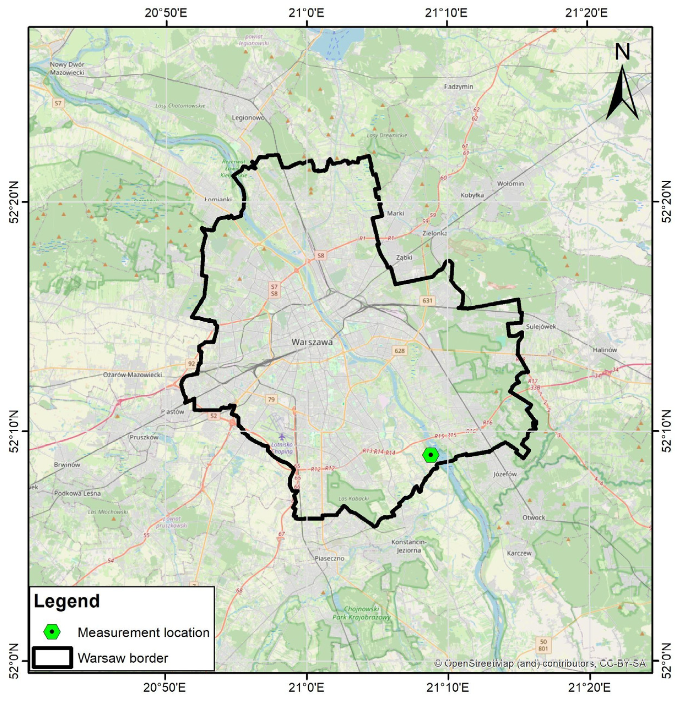
2.1. Study Area

The measurements were carried out on a partially reclaimed heap of the Siekierki thermal power plant managed by PGNiG TERMIKA S.A., located in Warsaw (21°8′47″E; 52°8′59″N). The location of the measurements is shown on the map (Figure 1).

Although most of the area has been reclaimed, there are still uncovered ash dumps from the thermal power plant in this vicinity. The examined area included one of the landfill sites with an area of approximately 2 ha. It is located on the northeastern slope of the Zawada heap, the so-called Section 3. There are agricultural fields and single-family buildings to the west and a riparian forest to the east, in the vicinity of the heap. Due to the wind’s direction during the campaign, the operation of the landfill area with an active sandpit near the borders on the east did not affect the measurements of the heap.

2.2. Measurement Techniques

Vertical atmospheric soundings were conducted during the project, using a tethered aerostat equipped with instruments capable of measuring the concentrations of suspended particulate matter (PM2.5 and PM10), as well as black carbon (BC) concentrations. Additional measurements were carried out at a ground station at heights of 2 and 10 m above ground level (agl).

2.2.1. Ground Station

In the measurement area, a ground station was installed, equipped with the following.

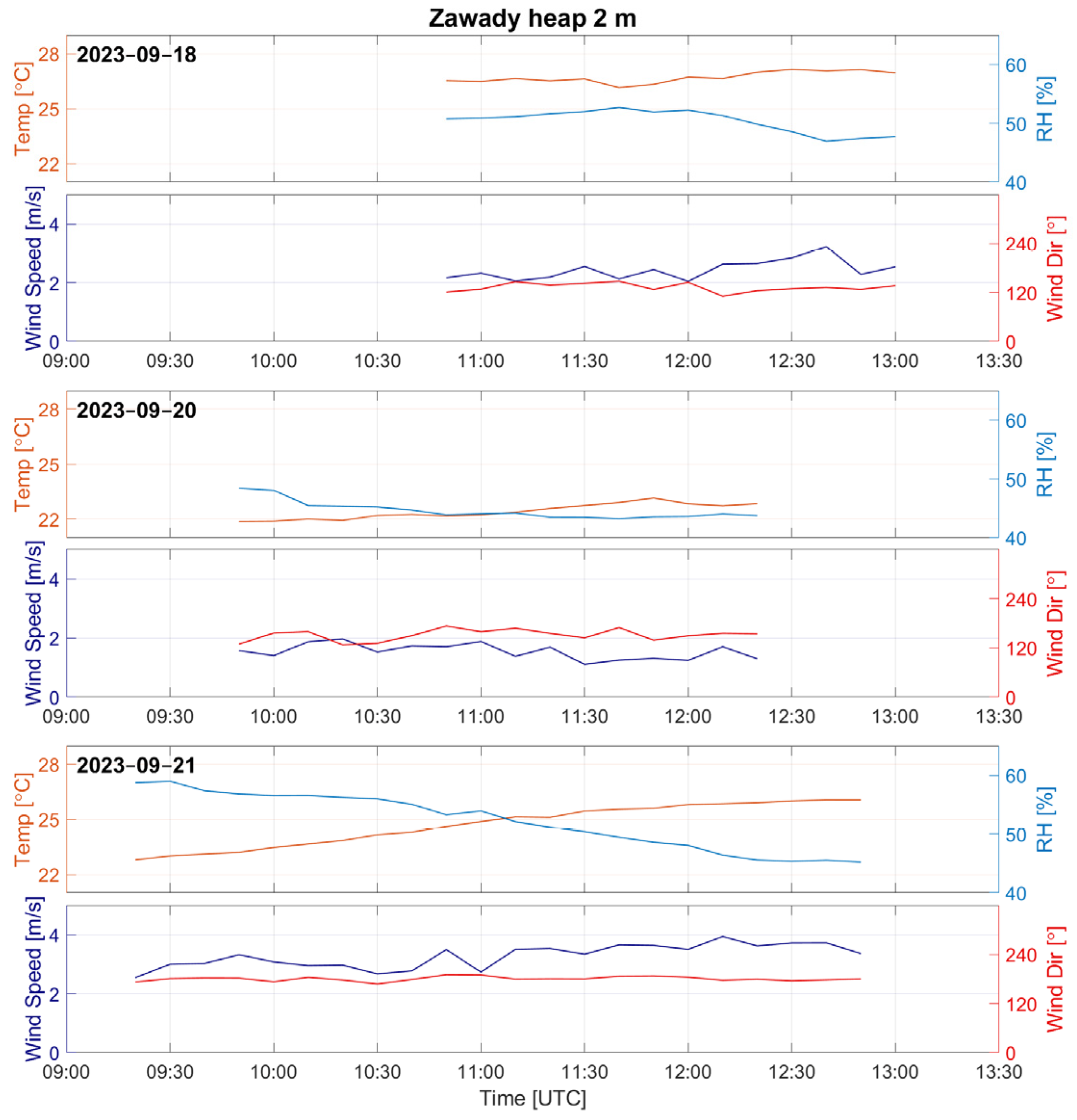
• A Gill MetConnect meteorological station measuring air pressure, temperature, humidity, and the wind’s direction and speed. It was placed 2 m agl, with the data recorded at a temporal resolution of 1 s.
• A station for measuring the particle size distribution, equipped with an SPS30 sensor for measuring concentrations of suspended particulate matter (PM2.5 and PM10). The sensor, positioned 2 m above ground level, recorded data at a temporal resolution of 1 s. Additionally, the station recorded the temperature and relative humidity of the air entering the sensor.
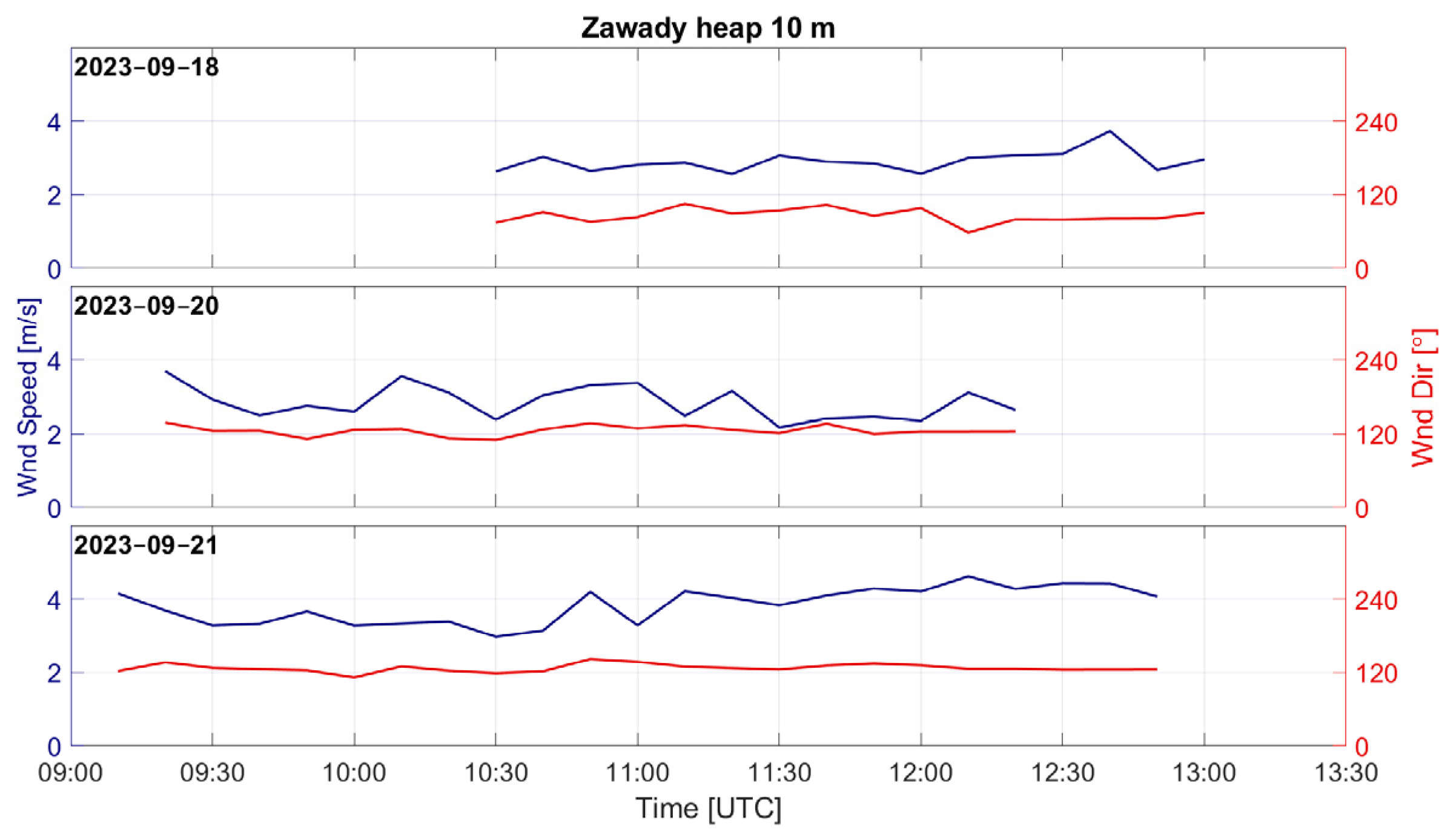
• An ultrasonic anemometer (Anemometer TriSonica), positioned at a height of 10 m agl, measuring three components of wind speed at a temporal resolution of 10 Hz.

2.2.2. Flying Measurement Platform

For vertical profiling of PM2.5, PM10, and BC, a MoniKite tethered aerostat was used as the measurement platform [33]. The length of the aerostat used was 8 m, with a maximum payload of 5 kg. Due to its proximity to Warsaw Chopin Airport (EPWA), flights were restricted to a maximum altitude of 250 m.

The payload of the aerostat consisted of equipment for studying the properties of atmospheric aerosols. The set included an optical particle counter (SPS30) for measuring particle size distribution and the concentrations of particulate matter (PM2.5 and PM10), as well as a counter for measuring the concentration of BC (AE51). The aerostat was equipped with a complete set of meteorological sensors for measuring the air temperature, relative humidity, and atmospheric pressure. Additionally, a GPS receiver was mounted. The sensors onboard the aerostat recorded data at a temporal resolution of 1 s.

2.3. Parameterization of Emission Fluxes

2.3.1. Description of the Selected Parameterization Method

The gradient method [34] was used to estimate aerosol fluxes. This method served as a parallel technique to the eddy covariance method. In the eddy covariance method, the flux is directly determined from measurements based on the covariance calculated between the fluctuations of a selected meteorological scalar (e.g., temperature, the concentration of gas, or the concentration of aerosols) and the vertical component of fluctuations in wind velocity. In contrast, the gradient method estimates the flux based on the concentration gradient of aerosols.

2.3.2. Theoretical Foundations

As mentioned in the introduction, turbulent diffusion is the dominant process in the atmospheric boundary layer. It is primarily responsible for the vertical transport of mass to higher altitudes. Conversely, the gravitational settling of aerosol particles is responsible for their removal. The concentration of aerosols can be decomposed into a mean and a fluctuating component using Reynolds decomposition: $n\left(D_p\right)=\overline{n\left(D_p\right)}+n’(D_p)$. After applying the same decomposition to the vertical component of wind velocity, the turbulent flux of particles and the settling flux can be expressed as

$$f_t\left(D_p\right)=\overline{n^{\prime }\left(D_p\right)·w^{\prime }}$$

(1a)

$$f_d\left(D_p\right)=V_g\left(D_p\right)·\overline{n\left(D_p\right)}$$

(1b)

where w′ represents the fluctuating vertical velocity of wind and Vg denotes the gravitational settling velocity of the particles.

The overbar in the notation above denotes the time averaging of the fluctuations over the measurement period, which is justified by the assumption of the ergodicity of the parameters. Assuming horizontal homogeneity, expanding and differentiating the general transport equation for particles, and assuming a zero mean for the component of wind velocity, we can write:

$$\overline{n^{\prime }\left(D_p\right)·w^{\prime }}+V_g\left(D_p\right)·\overline{n\left(D_p\right)}=const.$$

(2)

This equation satisfies the principle of constant fluxes in the boundary layer. On the basis of this equation, we concluded that to obtain the correct balance of the transported mass, we needed to determine its two components (a positive value denotes emission, and a negative value denotes deposition).

Using the M-O theory, we can define the scale of the concentration of aerosols as

$$N_{*}=\frac{F}{u_{*}}$$

(3)

where F denotes the aerosol flux and u_⁎ represents the friction velocity. On the basis of this scale, we can define a dimensionless concentration gradient scale as a function of the parameter ζ:

$$\frac{z}{N_{*}}\frac{\partial N}{\partial z}=\Phi (\zeta )$$

(4)

Integrating the expression over the height in the limits from z₂ to z₁, we obtained

$$N\left(z_2\right)-N\left(z_1\right)=N_{*}\left[\phi \left(\frac{z_2}{L}\right)-\phi \left(\frac{z_1}{L}\right)\right]$$

(5)

where φ is the primitive function of z⁻¹Φ(ζ).

According to the M-O theory, a logarithmic asymptote of the function φ is assumed for any ζ approaching zero. Therefore, we can finally write the formula for the vertical distribution of the concentration of aerosols as:

$$N\left(z\right)=N_{*}lnln\left(z\right)+C.$$

(6)

On the basis of the relationship above, it is possible to determine the dimensionless parameter Ψ given the horizontal distribution of the concentration of aerosols (profile), while the flux itself can be determined using Formula (3).

2.3.3. Limitations of the Method

The application of this technique requires us to acknowledge certain limitations. In its present form, the method assumes neutral atmospheric stability and a neutral gradient profile for the concentration. While there are numerous descriptions of the boundary layer for other types of atmospheric stratification (e.g., Sorbjan [35]), they focused on classical scalars describing the boundary layer (temperature, humidity). There is a lack of research specifically addressing the direct relationship between the profile of aerosols and turbulent diffusion coefficients for different types of atmospheric stability.

In the case of meteorological measurements, it is also crucial to operate within appropriate time scales. For the eddy covariance method, it is assumed that measuring a single flux requires at least 30 min to cover the entire spectral range of turbulent eddies. In the case of the gradient method applied in this study, this aspect is less significant, as the measurement involves calculating the gradient based on the average concentrations of aerosols. However, the necessity of capturing the forced secondary emissions from the spoil heap compelled us to shorten the time scale.

When conducting measurements of the turbulence, it is also important to consider larger time scales of variability. Measuring a single flux requires the observation of the entire cross-section of turbulent eddy sizes, which is why a 30-min measurement period was chosen. This allowed the capture of the variability of the inertial subrange in the spectral space of turbulence. However, to investigate the variability and physical processes influencing the transport processes, significantly longer periods of observation are required. From the perspective of basic micrometeorological processes, the absolute minimum appears to be the synoptic time scale, which is approximately 7 days. Planning such measurements offers the opportunity to observe various classes of wind speed and, consequently, the turbulent processes occurring at different levels.

2.3.4. Parameterization Calculations Based on the Measurements

The first step in calculating the fluxes was to determine the concentration gradient of the aerosols using Equation (6). This process entailed computing the N_⁎ values, which corresponded to calculating the linear regression coefficients of the straight line fitted between the concentration profiles of mass and the natural logarithm of the measurement height. The slope of such a line is denoted N_⁎.

The aerosol fluxes were calculated via Formula (3). For this purpose, it was necessary to estimate the friction velocity u_⁎. For the needs of this work, the formula proposed by Plate [36] and confirmed in the literature [37] was used

$$u_{*}=\frac{\kappa \underset{\_}{u}(h)}{ln(h/z_0)}.$$

(7)

where κ = 0.41 is the von Karman constant, $\underset{\_}{u}$ is the average wind speed at height h, and z₀ is the roughness parameter; for the needs of this work, a value of 10⁻³ was assumed, which corresponds to a flat sandy surface [38].

The determined fluxes were compared with the average wind speeds, and the function of the sources of aerosol emissions was determined. For the needs of this work, linear regression was used to obtain a simple relationship between wind speed and aerosol fluxes for the case of no forced emissions and for the case of forced secondary emissions.

2.4. GEM-AQ Model

The national air quality modelling system based on the GEM-AQ model [9] was used for this study. GEM-AQ is a semi-Lagrangian chemical weather model in which air quality processes (chemistry and aerosols) and tropospheric chemistry are implemented online in a weather prediction model, the Global Environmental Multiscale (GEM) [39] model, which was developed by Environment Canada. The gas-phase chemistry mechanism used in the GEM-AQ model is based on a modified version of the acid deposition and oxidants model (ADOM) [40], where additional reactions in the free troposphere are included. Aerosol processes are represented by parameters of nucleation, coagulation, and intra-cloud processes, including liquid phase chemistry for sulfur compounds and leaching inside the cloud, as well as sedimentation, and dry and wet deposition. Transport processes include advection, turbulence diffusion, and deep convection. The distribution of mass is represented in 12 particle size ranges of aerosols, describing the logarithmic increase in the particles’ radius. The modelled values of PM10 and PM2.5 concentrations were calculated as the sum of the fractions of the individual chemical components. The model has been evaluated in several research projects [10,41,42,43].

Since 2018, the model has been used for the national air quality forecasts and assessments for the Chief Inspectorate of Environmental Protection and operates as a partner model in the Copernicus Atmosphere Monitoring Service—Regional Production (CAMS2_40) [H]. Emission data for Poland are stored in the Central Emission Database, which was compiled using a high-resolution bottom-up inventory developed and maintained by the National Centre for Emission Management. For the energy production sector and industry, the data are based on annual reporting by facilities. The methodology for modelling residential emissions was described in [17]. Annual emissions are transformed into monthly emission rates using weighting factors from annual emission profiles. Emission profiles are assigned to the Standard Nomenclature for Air Pollution (SNAP) categories [44]. Computations were performed using a grid with a 0.025-degree resolution. The GEM-AQ model is set up to perform calculations using 28 vertical layers. The lower 21 layers are in the troposphere. The hourly output of PM2.5 and PM10 concentrations from the surface layer were used to calculate averages and comparisons with fields calculated to support the air quality policy in Poland (Environmental Protection Act, Art 86, Paragraph 6).

3. Results

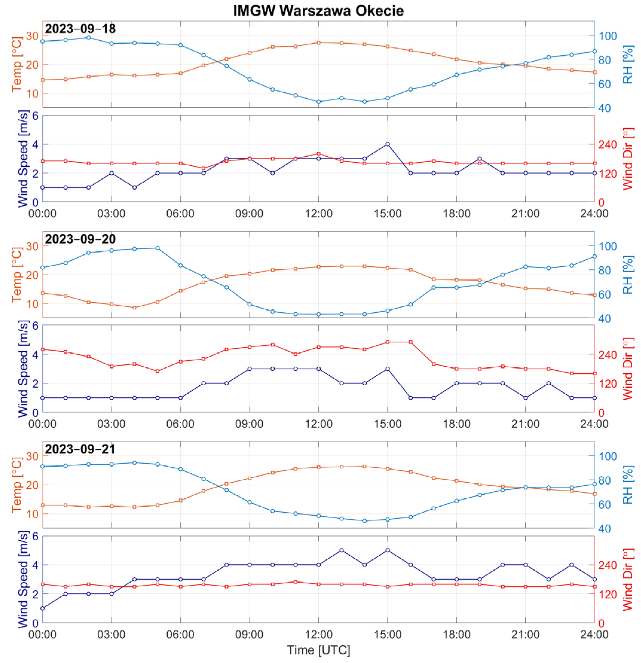
3.1. Variability in the Meteorological Conditions in the Warsaw Region

The weather conditions from the IMGW Warsaw Okecie station (12 km from the measurement site, 1 h time resolution) are presented in Figure 2. The temperature trends during the measurement days were quite similar. Air temperatures ranged at about 8–12 °C at night and in the early morning. During the day, temperatures reached maximums of 22–28 °C. Relative humidity fluctuated from approximately 95% during the night and early morning to about 40% during the day. On 18 and 21 September 2023, the prevailing wind was from the ESE direction, while on 20 September 2023, the dominant wind direction was from the SSW–SW direction. Wind speeds during the measurement period on the heap ranged from a minimum of 1–2 m/s to a maximum of 4–6 m/s. While the measurements were taken, no precipitation was present.

Figure 3 shows the meteorological conditions at the measurement site on the Zawady heap: the air temperature, relative humidity, wind direction, and wind speed. On 18–21 September 2023, temperatures reached 23–26 °C, while humidity fluctuated between 40% and 60%. The wind varied from 1 to 4 m/s from the ESE direction. The consistent wind direction in the recorded data resulted from the terrain’s features at the measurement site.

The wind direction and wind speed measured at 10 m on the measurement days are presented in Figure 4. The variability in both wind direction and wind speed recorded at the height of 10 m was similar to the trends observed at 2 m above ground level; however, the speed was approximately 1–2 m/s higher than at the ground station. The wind direction at 10 m shifted approximately 20° westward compared with the ground station.

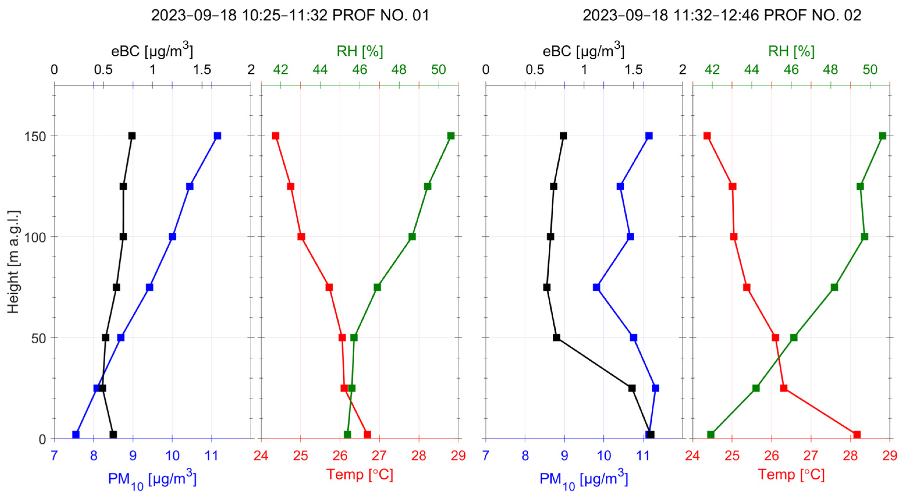
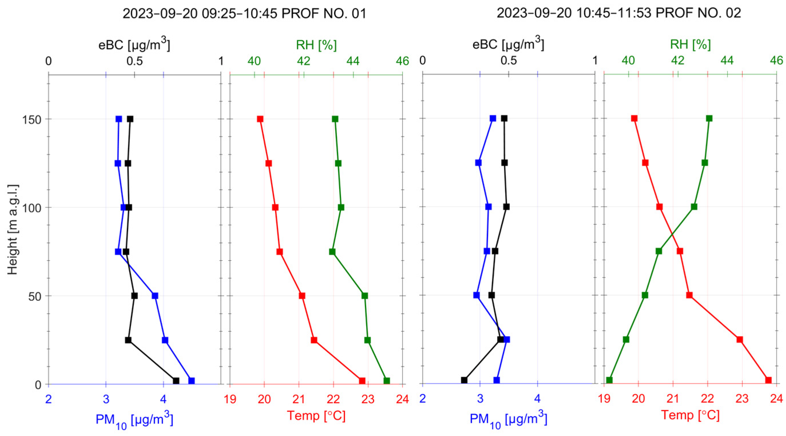
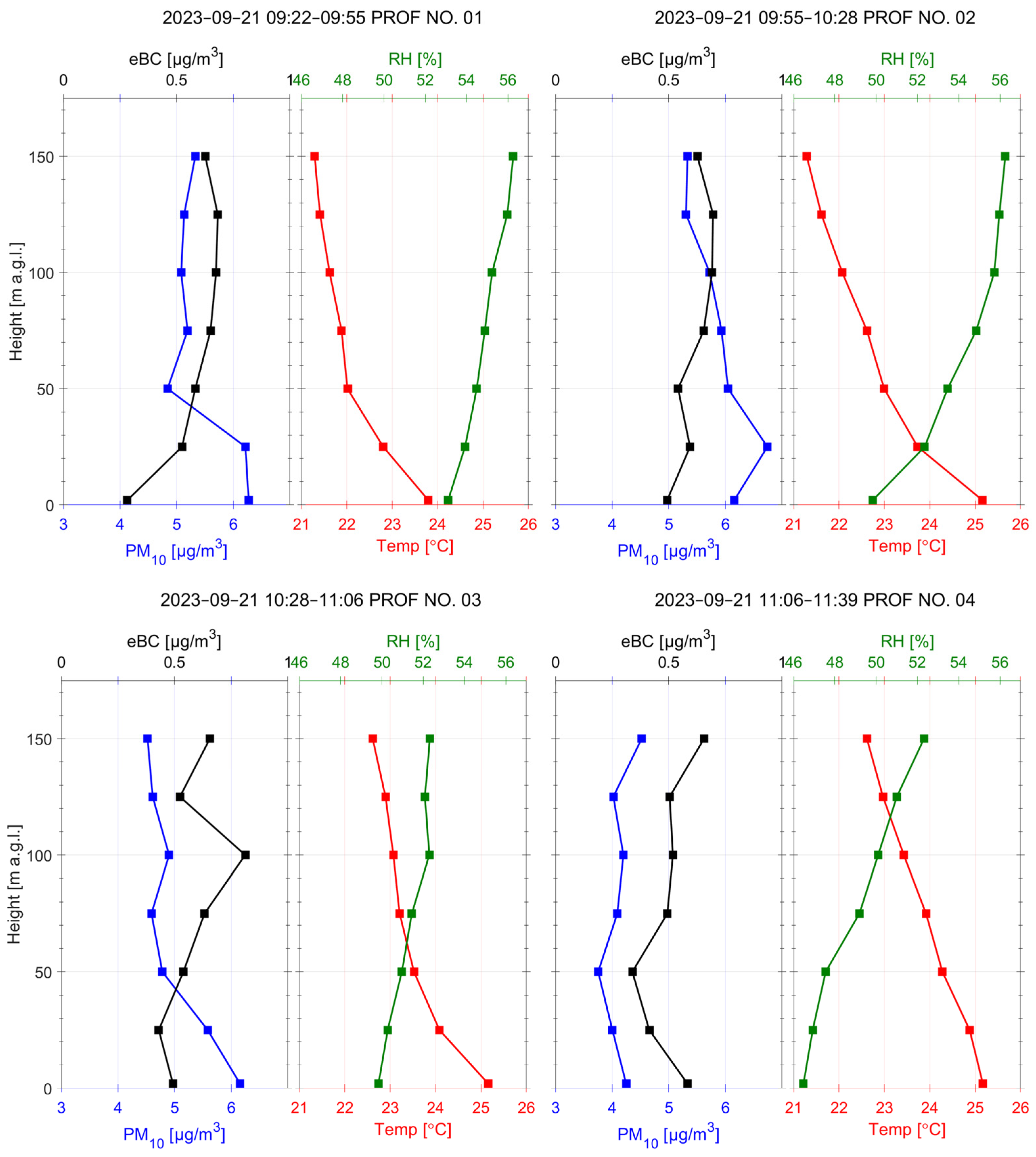
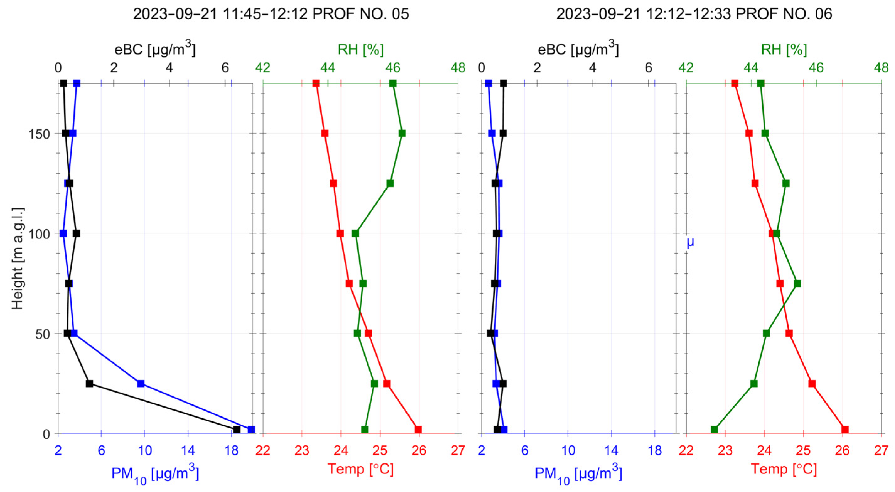
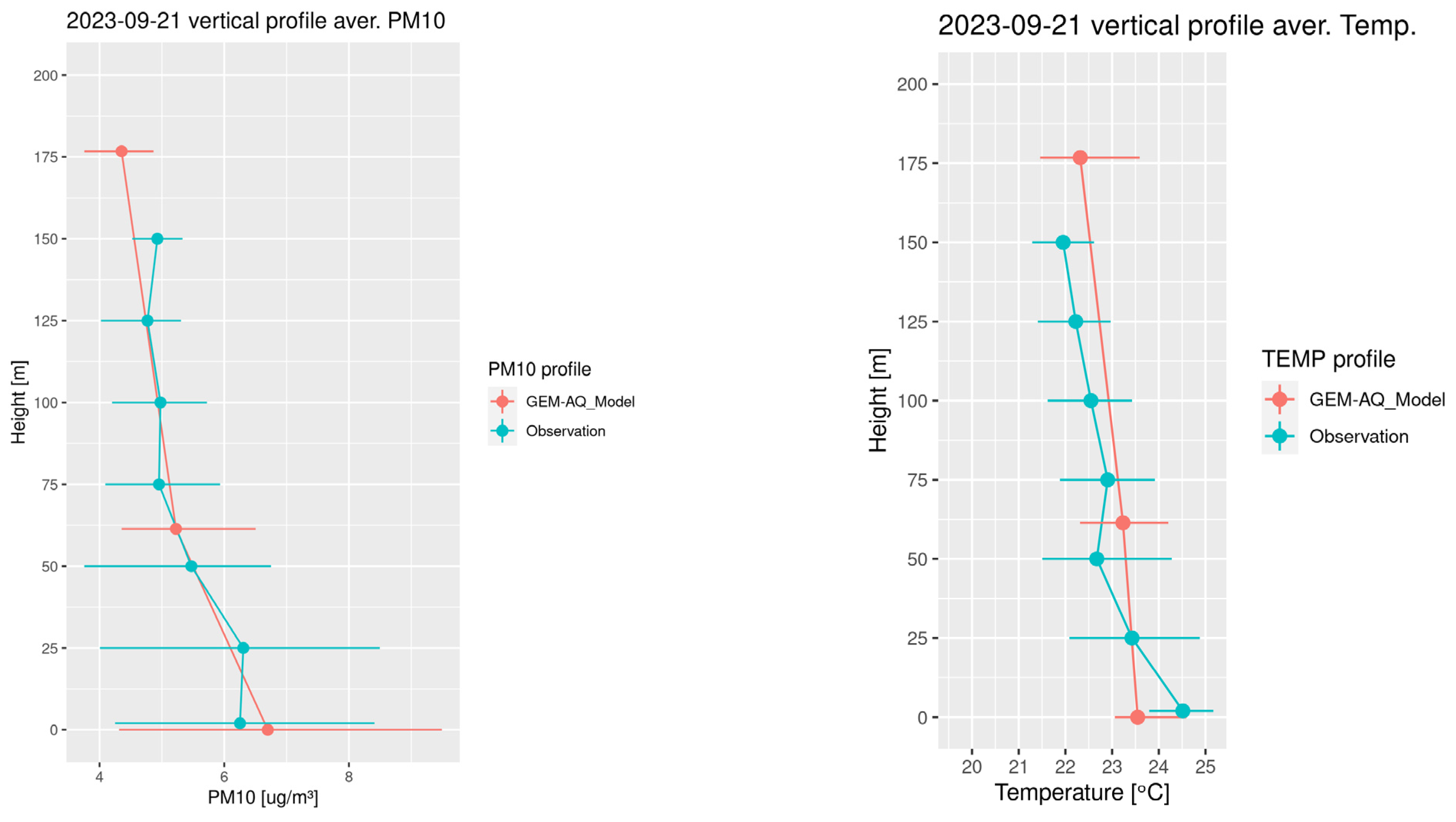
3.2. The Vertical Variability of Concentrations of PM2.5, PM10, and BC

In the following section, the results of atmospheric profiling using the MoniKite aerostat are presented. Measurements were taken every 25 m. The aerostat stayed at each level for 5 to 10 min, depending on the conditions.

On 18 September, two vertical profiles were measured up to a height of 150 m (Figure 5). The first profile was measured in an undisturbed area of the landfill. The ground-level concentration of BC was higher than the concentration of BC at 25 m. During the second profile, vehicle movements occurred in the landfill area. Profile 2 clearly showed dust rising to a height of 50–70 m, which was noticeable in the profiles of PM2.5, PM10, and BC.

It is worth noting that in all profiles and measurement data, the concentrations of PM2.5 and PM10 have identical values, indicating small particle sizes.

On 20 September 2023, two profiles were evaluated (Figure 6). The first profile showed a decrease in concentrations the of BC, PM2.5, and PM10, with concentrations three times lower than the previous day’s measurements.

For the profiles of 21 September 2023 (Figure 7), a decrease in the PM10 concentration was visible up to 50 m above ground level in the first profile and up to 125 m in the second profile. In the profiles of the BC concentration, an increase in concentrations was observed at ground level (Profiles 3 and 4) as well as in the altitude range of 50–100 m above ground level.

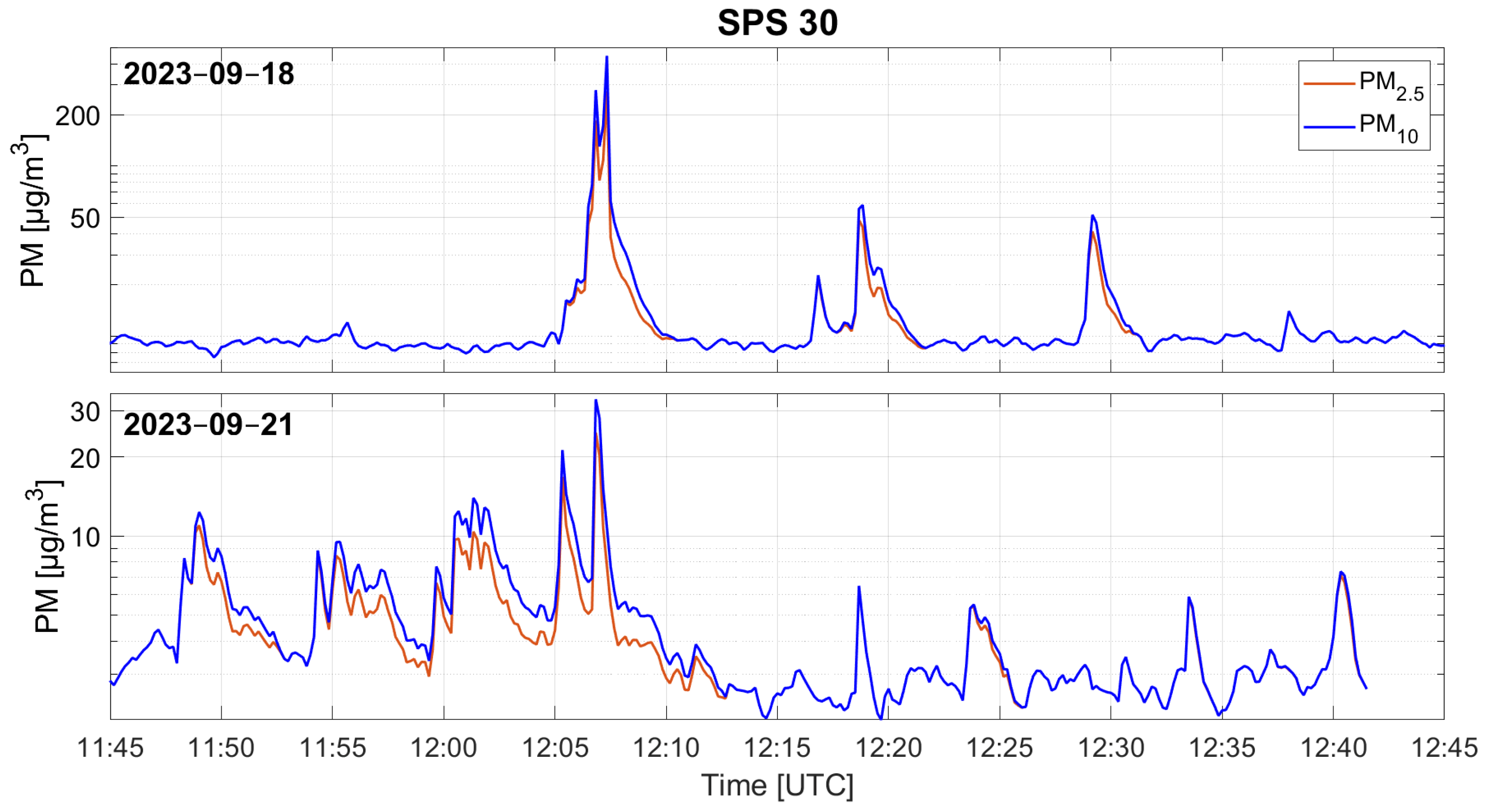
3.3. The Variability in PM2.5 and PM10 Concentrations during Vehicle Movements

During the measurements, a test was conducted to examine the impact of vehicle movements within the landfill area on emissions. This involved driving a car in the southern part of the landfill while conducting soundings. These tests were carried out on 18 and 21 September 2023.

Figure 8 shows the profiles of the PM2.5 and PM10 concentrations recorded at a height of 2 m above ground level. The upper panels depict data from 18 September 2023. Three vehicle passes were made around 12:06, 12:18, and 12:29 UTC. In the lower panel, data from 21 September 2023 are presented, showing four vehicle passes at approximately 11:48, 11:54, 12:00, and 12:04.

It is worth noting that only measurements taken during the machine’s operation showed a visible differentiation between the PM2.5 and PM10 fractions. This related to the appearance of larger particles (with a diameter larger than 2.5 μm).

In the profiles from the aerostat (Figure 9), there was a clear increase in the concentrations of PM2.5, PM10, and BC in the surface layer up to a height of 50 m above ground level. This profile was evaluated up to a height of 220 m above ground level. Fluctuations in the concentrations of BC, PM2.5, and PM10 with height were visible, consistent with the previous profiles from 21 September 2023. After the vehicle had passed, an additional profile was recorded, showing minimal changes in the surface layer.

3.4. Measurement—Conclusions

The measurements conducted at the Zawady landfill were pilot studies. They allowed us to test measurement techniques and technical solutions for such measurements.

A crucial aspect when conducting these measurements is selecting the location. The landfill should be situated away from other emission sources, such as cities or production facilities. Additionally, the landfill should be devoid of vegetation cover, as it significantly reduces surface emissions.

Weather conditions in the days before measurements are also a non-trivial issue. Precipitation notably increases the surface humidity of the landfill, leading to a notable reduction in dust emissions. When conducting such measurements, it is essential to measure soil moisture.

For the measurements at the Zawady landfill, a single ground station was utilized, which was situated on the windward side. For longer measurement campaigns, it is recommended to deploy a network of monitoring stations equipped with sensors for measuring PM2.5, PM10, BC, wind speed, wind direction, and basic meteorological data. These stations should be placed in a star-shaped pattern around the landfill and at a certain distance from it to observe the dispersion of dust depending on the wind direction.

The vertical soundings using a tethered aerostat conducted between 18 and 21 September 2023 indicated that dust from the landfill rose to about 50 m. It would be worthwhile to investigate how quickly it descends and how far it is transported. Hence, conducting additional vertical soundings at a distance from the landfill on the windward side is suggested.

3.5. Results of Parameterization

The results of calculating the aerosol fluxes are presented below. The results are divided into two types of fluxes, PM2.5 and PM10, which are marked on the graphs. The vertical axes in the description of the time series are marked with F_m, which refers to the English term “mass flux”.

For the measurement series without forced secondary emissions, the maximum values of aerosol flux were 0.0144 µg/s/m² and 0.0144 µg/s/m² for PM2.5 and PM10, respectively. The minimum values were −0.0327 µg/s/m² and −0.0327 µg/s/m². A positive value represents emissions, while a negative value represents deposition of aerosols.

In the case of measurements during the initiation of secondary emissions (with movement of a vehicle), the maximum values were 0.2217 µg/s/m² and 0.3636 µg/s/m², and the minimum values were −0.4064 µg/s/m² and −0.6713 µg/s/m².

As can be seen, the differences between the case without disturbance and the situation of forced emissions were high. To show the mutual relationship, the values presented above were divided by each other. The ratio of the maximum values was 16 and 25, and the ratio of the minimum values was 12 and 21. This means that in the case of PM10, the values of emissions in the case of disturbance of the spoil heap were 25 times higher, and for PM2.5, they were 12 times higher.

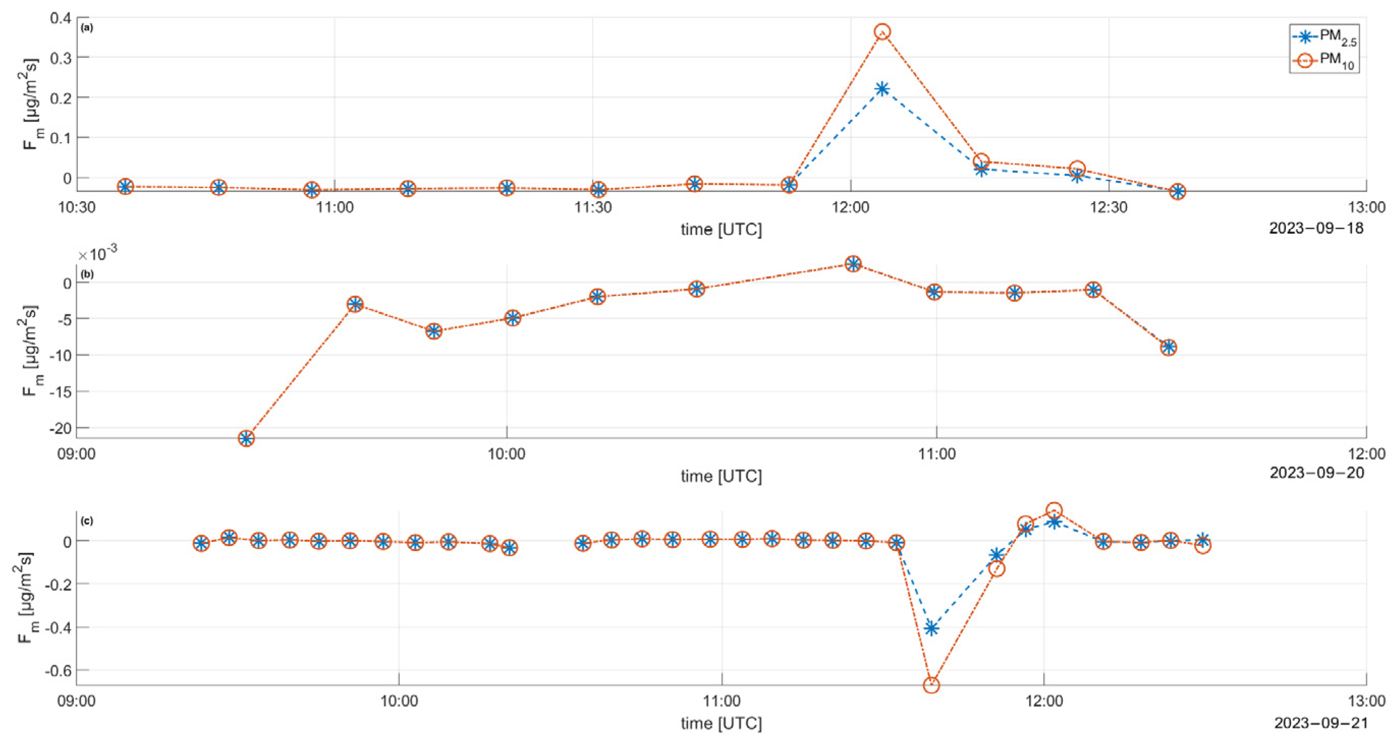
3.5.1. Description of the Time Series of Flux

Figure 10 presents the temporal variability of the aerosol fluxes determined during three consecutive days of the measurement campaign. Across all three measurement periods, without forced emissions, we observed very low aerosol fluxes, predominantly indicating the deposition of aerosols. This suggests a stable process of advection and deposition of aerosols from urban areas.

In Figure 10, for the case of 18 September, after 12:00, we observed a sharp increase in emissions caused by the initiation of secondary emissions induced by a moving vehicle. The initiated emissions decreased further during the measurement period, eventually returning to values close to the initial ones. On 20 September, we observed a very low mass exchange, with a prolonged period of weak deposition of aerosols, likely influenced by advection.

In the first part of the measurements on 21 September until 11:30, a low exchange was observed again, with a dominance of deposition of aerosols. After 11:30, we first observed a very strong negative aerosol flux, followed by an emission of a slightly smaller magnitude. This likely occurred because the cloud of resuspended dust initially reached the sensor on the aerostat. Later, with the progressive dispersion of the particles, the pollution signal also reached the sensor located on the measurement tower. This observation was crucial, as it highlighted how the measurements’ time scale can affect the measurement of dust transported in the surface layer, particularly when the turbulence conditions are not well developed.

The convergent values for both measurement ranges during periods without forced emissions suggested the presence of smaller particles. The emission of particles larger than 2.5 microns only occurred during forced emissions.

3.5.2. Dependence of Flux on Wind Speed—Parametrization of Dust Emissions

Figure 11 presents the relationship between the measured aerosol emissions and wind speed. The results are presented using the convention of dividing the fluxes into periods without forced secondary emissions (blue color) and during emissions (red color).

For each case, a linear function was fitted to the data using the linear regression method according to the formula

$$F_{PMx}\left(u\right)=a_{x}u+b_x$$

(8)

where x denotes the size range (PM2.5 and PM10), and the coefficients a and b are the linear fitting coefficients presented in

Table 1. Linear fitting coefficients representing the functions of the sources of aerosol emissions according to Formula (8). The subscript w refers to emissions from mechanical disturbance of the aerosol. The functional dependencies are fitted to the calculated values of dust flux and therefore allow for estimation of the emissions in units of µg/s/m².

	ax	bx
FPM10 (u)	0.0017	−0.0007
FPM2.5 (u)	0.0017	−0.0007
FwPM10 (u > 2.5 m/s)	0.0272	0.0038
FwPM10 (u < 2.5 m/s)	0.0049	0.0582
FwPM2.5 (u)	0.0041	0.0492

. The subscript PM with a tilde indicates a linear fit to the data measured during secondary resuspension of aerosols. For wind speeds lower than 2.5 m/s, we assumed the same rate of decrease for both size ranges, which has been marked in the brackets of the functions.

The figure shows that the fitted functional relationships describing the aerosol flux during forced emissions were an order of magnitude higher than those in the absence of secondary emissions. The ratio of the averaged values of the functions representing the secondary emissions F_wPM10 to F_wPM2.5 was 1.6, which indicated that the observed PM10 emissions were almost twice as high as the PM2.5 emissions.

Another conclusion from the developed fitting is that the functions F_PM2.5 and F_PM10 were identical. This is because smaller particles dominated in the absence of forced emissions, as mentioned in the previous subsection.

3.6. Calculation of Emissions

To calculate emissions from all heaps in Poland, the following data and assumptions were used:

• Developed parameterization,
• Average daily wind speed fields from the GEM-AQ model for 2022, and
• Outlines of heaps and workings from BDOT.

The average daily wind speed was adjusted to each heap’s outline, using the GIS tool. Several scenarios were calculated to obtain the daily and yearly emissions for all heaps/dumps in Poland using defined parameterization:

• No commotion,
• Commotion for 8 h a day but only on working days (252 working days),
• Commotion for 8 h for 365 days, and
• Continuous commotion

The equations used to calculate the annual emissions for a specific facility for each scenario were as follows.

• No commotion
• For PM10:

  $$E_{PM10}={\sum }_{i=1}^{365}{F}_{PM10}\ast 24\ast A\ast 3600\ast {10}^{-9}\left[\frac{kg}{y}\right]$$

  (9)
• For PM2.5:

  $$E_{PM2.5}={\sum }_{i=1}^{365}{F}_{PM2.5}\ast 24\ast A\ast 3600\ast {10}^{-9}\left[\frac{kg}{y}\right]$$

  (10)
• Commotion for 8 h a day but only on working days (252 working days)
• For PM10:

  $$E_{PM10}=({\sum }_{i=1}^{256}{F}_{wPM10}\ast 8+{\sum }_{i=1}^{256}{F}_{PM10}\ast 16+{\sum }_{i=1}^{109}{F}_{PM10}\ast 24)\ast A\ast 3600\ast {10}^{-9}\left[\frac{kg}{y}\right]$$

  (11)
• For PM2.5

  $$E_{PM25}=({\sum }_{i=1}^{256}{F}_{wPM2.5}\ast 8+{\sum }_{i=1}^{256}{F}_{PM2.5}\ast 16+{\sum }_{i=1}^{109}{F}_{PM2.5}\ast 24)\ast A\ast 3600\ast {10}^{-9}\left[\frac{kg}{y}\right]$$

  (12)
• Commotion for 8 h for 365 days
• For PM10:

  $$E_{PM10}=({\sum }_{i=1}^{256}{F}_{wPM10}\ast 8+{\sum }_{i=1}^{256}{F}_{PM10}\ast 16+{\sum }_{i=1}^{109}{F}_{PM10}\ast 24)\ast A\ast 3600\ast {10}^{-9}\left[\frac{kg}{y}\right]$$

  (13)
• For PM2.5:

  $$E_{PM25}=({\sum }_{i=1}^{256}{F}_{wPM2.5}\ast 8+{\sum }_{i=1}^{256}{F}_{PM2.5}\ast 16+{\sum }_{i=1}^{109}{F}_{PM2.5}\ast 24)\ast A\ast 3600\ast {10}^{-9}\left[\frac{kg}{y}\right]$$

  (14)
• Continuous commotion
• For PM10:

  $$E_{PM10}={\sum }_{i=1}^{365}{F}_{wPM10}\ast 24\ast A\ast 3600\ast {10}^{-9}\left[\frac{kg}{rok}\right]$$

  (15)
• For PM2.5:

  $$E_{PM25}={\sum }_{i=1}^{365}{F}_{wPM2.5}\ast 24\ast A\ast 3600\ast {10}^{-9}\left[\frac{kg}{rok}\right]$$

  (16)
• In all these formulae,

  F_PM10 = 0.0017 × u − 0.0007

  F_PM2.₅ = 0.0017 × u – 0.0007

  F_wPM10 (u > 2.5 m/s) = 0.0272 × u + 0.0038

  F_wPM10 (u < 2.5 m/s) = 0.0049 × u + 0.0582

  F_wPM2.5 = 0.0041 × u − 0.0492

  where u is the average daily speed for the selected object (m/s) and A is the area of the selected object (m²).

In

Table 2. Quantity of yearly emissions in Poland calculated using parameterization and from the CED.

Emission Scenarios	PM10 [kg]	PM2.5 [kg]
No commotion	42,470	42,470
Commotion for 8 h a day but only on working days (252 working days)	236,364	217,674
Commotion for 8 h for 365 days	399,946	297,921
Continuous commotion	886,289	803,893
CED 2022	9,493,354	2,283,012

, the annual emissions of PM10 and PM2.5 from all heaps in Poland under various scenarios and from the CED are presented. In all scenarios, the calculated emissions were significantly lower than those from the CED. The parametrization above gives estimations of the emissions that are several times lower than the previously used parameterization [18], which predicted emissions of PM2.5 and PM10 dust at levels of 760 and 169.4 kg/ha/year, respectively.

A modelling scenario with 8 h of commotion for 365 days was chosen.

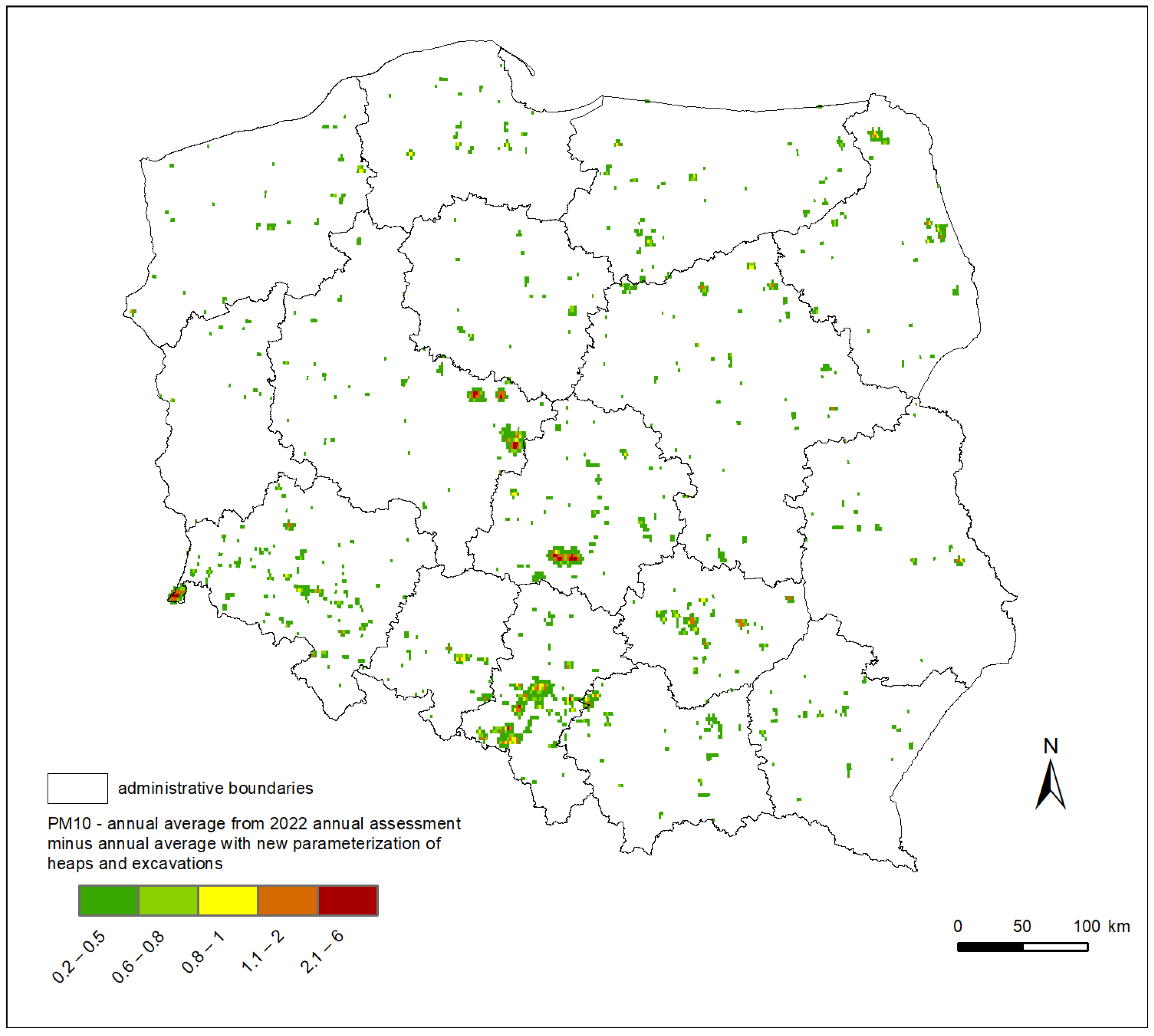
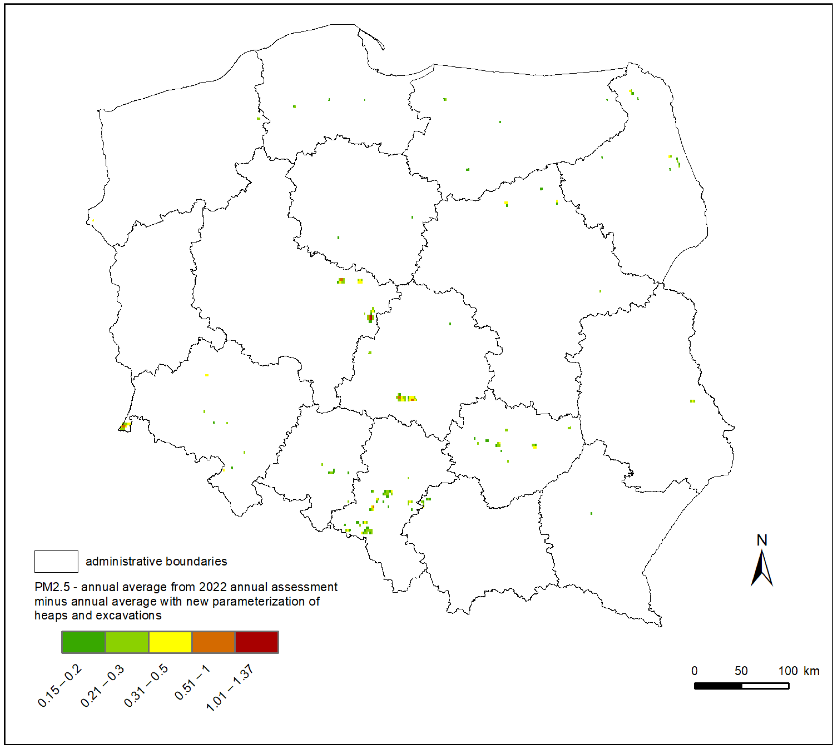
3.7. Modelling Results

Modelling simulations were conducted to calculate the differences in the particulate matter pollution resulting from changes in emissions from heaps and excavations. The national air quality modelling system based on the GEM-AQ model was used, with an updated CED, taking the parametrization described in Section 3.5 into account. Yearly average concentrations were calculated and compared with fields from simulations carried out within the scope of the annual national assessment for 2022 (Figure 12 and Figure 13).

The differences in the annual concentration of PM10 occurred primarily in the locations of heaps and excavations (Figure 12); as expected, they were proportional to their size. Most of the calculated differences ranged from 0.2 to 0.8 µg/m³. The highest was noticed in the vicinity of the largest national power plants and large industrial areas, ranging from 2 to 6 µg/m³, which may relate to a significant part of the total PM10 concentration modelled in these areas over a year.

The differences in the annual PM2.5 concentration were significantly smaller compared with those of PM10 and were primarily noticeable around the largest heaps and excavations in Poland (Figure 13). Annual concentrations from simulations based on emissions using the new parameterization differed by 0.15 to 0.5 µg/m³ compared with the concentrations calculated for the annual assessment for the year 2022. The most significant differences, reaching 0.5 to 1.4 µg/m³, were rarely seen and were concentrated in individual grid cells.

Furthermore, additional modelling simulations were calculated for the days when the measurement campaign was conducted. The following charts (Figure 14) compare the vertical measurement profiles of PM10 aerosols and air temperature obtained during the campaign with the results of the model simulations performed for the project. Measurements were taken every 25 m up to a height of 150 m. Approximately within this height range, the GEM-AQ model computed results for three layers with average heights of 2 m, 67.5 m, and 177 m above surface level. Concentrations at individual levels, both for the model and observations, were averaged over time and represented as points, while outliers are shown as horizontal lines (whiskers).

Figure 14 indicates strong agreement between the modelled results and the measured values during all days of the campaign. The difference in the PM10 concentrations was slight and varied from 0.5 to 1.5 ug/m³. Temperature discrepancies did not exceed 0.5–1 °C. In the case of both parameters, vertical variability was maintained.

Good agreement between the modelling results and measurements could lead to the conclusion that the emissions of particulate pollutants calculated on the basis of the proposed parameterization largely reflect possible emissions from heaps and excavations. It is recommended to conduct an additional campaign and analysis considering diverse meteorological conditions, with measurements possibly conducted at multiple heaps.

4. Discussion

There are many methods for determining emissions from heaps and excavations, as mentioned in the introduction, but they require precise information, e.g., about the fraction, mineral composition, or physical parameters of the object (height, angle of inclination, etc.). The main aim of this research was to develop a method enabling the determination of emissions from heaps and excavations using the available meteorological and physical data for the entire area of Poland.

In this study, a ground measurement station located on the leeward side was used for measurements. In the case of a longer measurement campaign, it is suggested to set up a grid of measurement stations arranged in a star-like manner at a certain distance and equipped with sensors for measuring PM2.5, PM10, BC, wind speed, wind direction, and basic meteorological data. Vertical probing using an aerostat showed that dust from the landfill rose to a height of approximately 50 m. It is worth examining how quickly it falls and how far it is transported. Therefore, it is suggested to perform additional vertical soundings away from the heap on the leeward side.

The estimated volume of emissions is many times lower than that previously used in the CED. The research was performed in a relatively short period during stable meteorological conditions. Moreover, the analysis was based on the forced dust emissions generated by one vehicle driving around the heap. The campaign, unfortunately, did not allow for measurements at higher wind speeds, which are necessary to observe emissions caused by the turbulent exchange of momentum between the wind and the ground. The parameterization was therefore extrapolated to higher wind speeds. To verify the actual level of emissions and complete the parameterization, it is necessary to carry out more extensive measurements. The best method is the eddy covariance method, which will allow for real measurements of dust fluxes. It will also be possible to perform a detailed identification of the source area and determine the so-called footprint function [45,46].

Other meteorological parameters may also affect emissions and transport. For example, high humidity and precipitation can contribute to the suppression or even stop emissions of dust. Atmospheric stability can also affect the process of transporting dust in the boundary layer. In the case of a stable atmosphere, the emitted pollutants can remain in the spoil heap’s area for a longer time, negatively affecting the local air quality. In the case of an unstable atmosphere, better mixing and greater dispersion of the emitted dust cloud can be expected.

Considering the conclusions drawn above, it seems reasonable to conduct a more comprehensive measurement campaign spanning an extended period. This will allow measurements that cover various weather scenarios and provide a comprehensive understanding of emissions of dust from the heap.

The modelling results of emissions developed according to parameterization described above indicated a clear reduction in PM10 concentrations and a noticeable reduction in PM2.5 over the areas of heaps and workings compared with the data from the CED. In areas with a high density of heaps (e.g., Silesia), the emission levels previously used in the CED could account for several additional days with exceedances in the modelling results submitted as part of the annual assessment.

However, the results obtained using modelling showed very good agreement with the parameters measured during the campaign. This indicates that the emissions of dust calculated on the basis of the proposed parameterization closely reflect the actual emissions from heaps and excavations.

The developed results will be used to calculate annual emissions from mine heaps for the CED. A major advantage of the methodology is the ability to update the data annually with the average annual wind speed, location, and size of individual objects.

5. Conclusions

This study developed a method for estimating emissions from heaps and excavations. In this method, emissions depend on wind speed and the area of the object, making it straightforward in terms of the data requirements and universally applicable for determining emissions across an entire country. The estimated emission rate was several times lower than the previously used parameterization [18], which predicted emissions of PM2.5 and PM10 dust at levels of 760 and 169.4 kg/ha/year, respectively.

Due to such a large discrepancy, it is important to note a few key issues regarding the interpretation of the obtained results. The analysis was based on the forced emissions of dust generated by a single vehicle moving on the spoil heap. In the case of more vehicles operating on the spoil heap, significantly higher emissions than those presented in this report can be expected. The type of work of the machines and the type of vehicles (speed of movement, mass, characteristics of the tires) may also be important. Another very important aspect is the meteorological conditions. Additionally, other meteorological parameters, such as high humidity, precipitation and atmospheric stability, may also influence emissions and transport.

Taking the conclusions above into account, it seems reasonable to carry out another, more extensive measurement campaign over a longer time. This will allow us to include measurements of different weather scenarios and to provide a more complete picture of the phenomenon of dust lifting from the spoil heap. Due to the small number of such analyses in the literature, the research should be continued.

References

1. Manisalidis, I.; Stavropoulou, E.; Stavropoulos, A.; Bezirtzoglou, E. Environmental and Health Impacts of Air Pollution: A Review. Front. Public Health 2020, 8, 505570. [Google Scholar] [CrossRef] [PubMed]
2. Lelieveld, J.; Evans, J.S.; Fnais, M.; Giannadaki, D.; Pozzer, A. The contribution of outdoor air pollution sources to premature mortality on a global scale. Nature 2015, 525, 367–371. [Google Scholar] [CrossRef] [PubMed]
3. Künzli, N.; Kaiser, R.; Medina, S.; Studnicka, M.; Chanel, O.; Filliger, P.; Herry, M.; Horak, S., Jr.; Puybonnieux-Texier, V.; Quénel, P.; et al. Public-health impact of outdoor and traffic-related air pollution: A European assessment. Lancet 2000, 356, 795–801. [Google Scholar] [CrossRef] [PubMed]
4. Agency, E.E. Air Quality in Europe 2022; Web Report; European Environment Agency: Copenhagen, Denmark, 2022.
5. José, R.S.; Baklanov, A.; Sokhi, R.S.; Karatzas, K.; Pérez, J.L. Air Quality Modeling. Encycl. Ecol. Five-Vol. Set 2008, 111–123. [Google Scholar] [CrossRef]
6. Chang, J.C.; Hanna, S.R. Air quality model performance evaluation. Meteorol. Atmos. Phys. 2004, 87, 167–196. [Google Scholar] [CrossRef]
7. Rao, S.T.; Galmarini, S.; Puckett, K. Air quality model evaluation international initiative (AQMEII): Advancing the state of the science in regional photochemical modeling and its applications. Bull. Am. Meteorol. Soc. 2011, 92, 23–30. [Google Scholar] [CrossRef]
8. Silveira, C.; Ferreira, J.; Miranda, A.I. The challenges of air quality modelling when crossing multiple spatial scales. Air Qual. Atmos. Health 2019, 12, 1003–1017. [Google Scholar] [CrossRef]
9. Kaminski, J.W.; Neary, L.; Struzewska, J.; McConnell, J.C.; Lupu, A.; Jarosz, J.; Toyota, K.; Gong, S.L.; Côté, J.; Liu, X.; et al. GEM-AQ, an on-line global multiscale chemical weather modelling system: Model description and evaluation of gas phase chemistry processes. Atmos. Chem. Phys. 2008, 8, 3255–3281. [Google Scholar] [CrossRef]
10. Struzewska, J.; Zdunek, M.; Kaminski, J.W.; Łobocki, L.; Porebska, M.; Jefimow, M.; Gawuc, L. Evaluation of the GEM-AQ model in the context of the AQMEII Phase 1 project. Atmos. Chem. Phys. 2015, 15, 3971–3990. [Google Scholar] [CrossRef]
11. Russell, A.; Dennis, R. NARSTO critical review of photochemical models and modeling. Atmos. Environ. 2000, 34, 2283–2324. [Google Scholar] [CrossRef]
12. Clappier, A.; Thunis, P. A probabilistic approach to screen and improve emission inventories. Atmos. Environ. 2020, 242, 7823–7830. [Google Scholar] [CrossRef]
13. De Meij, A.; Cuvelier, C.; Thunis, P.; Pisoni, E.; Bessagnet, B. Sensitivity of air quality model responses to emission changes: Comparison of results based on four EU inventories through FAIRMODE benchmarking methodology. Geosci. Model Dev. 2024, 17, 587–606. [Google Scholar] [CrossRef]
14. Thunis, P.; Kuenen, J.; Pisoni, E.; Bessagnet, B.; Banja, M.; Gawuc, L.; Szymankiewicz, K.; Guizardi, D.; Crippa, M.; Lopez-Aparicio, S.; et al. Emission ensemble approach to improve the development of multi-scale emission inventories. Egusph. Prepr. Repos. 2023, 17, 3631–3643. [Google Scholar] [CrossRef]
15. Nazar, W.; Niedoszytko, M. Air Pollution in Poland: A 2022 Narrative Review with Focus on Respiratory Diseases. Int. J. Environ. Res. Public Health 2022, 19, 895. [Google Scholar] [CrossRef] [PubMed]
16. Agency, E.E. Poland—Air Pollution Country Fact Sheet. 2023. Available online: https://www.eea.europa.eu/themes/air/country-fact-sheets/2023-country-fact-sheets/poland-air-pollution-country (accessed on 10 May 2024).
17. Gawuc, L.; Szymankiewicz, K.; Kawicka, D.; Mielczarek, E.; Marek, K.; Soliwoda, M.; Maciejewska, J. Bottom–up inventory of residential combustion emissions in Poland for national air quality modelling: Current status and perspectives. Atmosphere 2021, 12, 1460. [Google Scholar] [CrossRef]
18. National Pollutant Inventory. National Pollutant Inventory Emission Estimation Technique Manual for Mining and Processing of Non-Metallic Minerals Version 2.1; Australian Government: Canberra, Australia, 2012; p. 45.
19. Ciszewski, A.; Wojciechowski, K. Metody obliczania stanu zanieczyszczenia powietrza atmosferycznego powodowanego przez źródła powierzchniowe. Ochr. Powietrza 1982, 6, 78–82. [Google Scholar]
20. Pastuszka, J.S. Emisja pyłu ze zwałowisk węgla i miału. Ochr. Powietrza I Probl. Odpad. 1996, 30, 43–47. [Google Scholar]
21. Zawadzka, O.; Posyniak, M.; Nelken, K.; Markuszewski, P.; Chilinski, M.T.; Czyzewska, D.; Lisok, J.; Markowicz, K.M. Study of the vertical variability of aerosol properties based on cable cars in-situ measurements. Atmos. Pollut. Res. 2017, 8, 968–978. [Google Scholar] [CrossRef]
22. Hinds, W.C. Aerosol Technology: Properties, Behaviour, and Measurement of Airborne Particles; Wiley: Hoboken, NJ, USA, 1982. [Google Scholar]
23. Monin, A.S.; Obukhov, A.M. Basic laws of turbulent mixing in the surface layer of the atmosphere. Geophys. Inst. Acad. Sci. USSR 1959, 24, 163–187. [Google Scholar]
24. Foken, T. Micrometeorology, 2nd ed.; Springer: Berlin/Heidelberg, Germany, 2017. [Google Scholar]
25. Mårtensson, E.M.; Nilsson, E.D.; Buzorius, G.; Johansson, C. Eddy covariance measurements and parameterisation of traffic related particle emissions in an urban environment. Atmos. Chem. Phys. 2006, 6, 769–785. [Google Scholar] [CrossRef]
26. Johansson, C.; Norman, M.; Gidhagen, L. Spatial & temporal variations of PM10 and particle number concentrations in urban air. Environ. Monit. Assess. 2007, 127, 477–487. [Google Scholar]
27. Harrison, R.M.; Dall, M.; Beddows, D.C.S.; Thorpe, A.J.; Bloss, W.J.; Allan, J.D.; Coe, H.; Dorsey, J.R.; Gallagher, M.; Martin, C.; et al. Atmospheric chemistry and physics in the atmosphere of a developed megacity (London): An overview of the REPARTEE experiment and its conclusions. Atmos. Chem. Phys. 2012, 12, 3065–3114. [Google Scholar] [CrossRef]
28. Kontkanen, J.; Deng, C.; Fu, Y.; Dada, L.; Zhou, Y.; Cai, J.; Daellenbach, K.R.; Hakala, S.; Kokkonen, T.V.; Lin, Z.; et al. Size-resolved particle number emissions in Beijing determined from measured particle size distributions. Atmos. Chem. Phys. 2020, 20, 11329–11348. [Google Scholar] [CrossRef]
29. Farmer, D.K.; Boedicker, E.K.; Debolt, H.M. Dry Deposition of Atmospheric Aerosols: Approaches, Observations, and Mechanisms. Annu. Rev. Phys. Chem. 2020, 72, 375–397. [Google Scholar] [CrossRef]
30. Patra, A.K.; Gautam, S.; Kumar, P. Emissions and human health impact of particulate matter from surface mining operation—A review. Environ. Technol. Innov. 2016, 5, 233–249. [Google Scholar] [CrossRef]
31. Field, J.P.; Belnap, J.; Breshears, D.D.; Neff, J.C.; Okin, G.S.; Whicker, J.J.; Painter, T.H.; Ravi, S.; Reheis, M.C.; Reynolds, R.L. The ecology of dust. Front. Ecol. Environ. 2010, 8, 423–430. [Google Scholar] [CrossRef]
32. Hvistendahl, M. Coal Ash Is More Radioactive than Nuclear Waste By burning away all the pesky carbon and other impurities, coal power plants produce heaps of radiation. Sci. Am. 2007, 13, 104–109. [Google Scholar]
33. Knap, L.; Świercz, A.; Graczykowski, C.; Holnicki-Szulc, J. Self-deployable tensegrity structures for adaptive morphing of helium-filled aerostats. Arch. Civ. Mech. Eng. 2021, 21, 159. [Google Scholar] [CrossRef]
34. Markuszewski, P.; Petelski, T.; Zielinski, T. Marine aerosol fluxes determined by simultaneous measurements of eddy covariance and gradient method. Environ. Eng. Manag. J. 2018, 17, 261–265. [Google Scholar] [CrossRef]
35. Sorbjan, Z. Structure of the Atmospheric Boundary Layer; Prentice Hall: Englewood Cliffs, NJ, USA, 1989. [Google Scholar]
36. Plate, E.J. Aerodynamic Characteristics of Atmospheric Boundary Layers; Argonne National Lab., Ill. Karlsruhe University: Karlsruhe, Germany, 1971; Volume 51, pp. 622–623. [Google Scholar]
37. Seinfeld, J.H.; Pandis, S.N. Atmospheric Chemistry and Physics: From Air Pollution to Climate Change, 3rd ed.; Wiley: Hoboken, NJ, USA, 2016. [Google Scholar]
38. McRae, G.J.; Goodin, W.R.; Seinfeld, J.H. Numerical solution of the atmospheric diffusion equation for chemically reacting flows. J. Comput. Phys. 1982, 45, 1–42. [Google Scholar] [CrossRef]
39. Côté, J.; Gravel, S.; Méthot, A.; Patoine, A.; Roch, M.; Staniforth, A. The operational CMC-MRB global environmental multiscale (GEM) model. Part I: Design considerations and formulation. Mon. Weather Rev. 1998, 126, 1373–1395. [Google Scholar] [CrossRef]
40. Venkatram, A.; Karamchandani, P.K.; Misra, P.K. Testing a comprehensive acid deposition model. Atmos. Environ. 1988, 22, 737–747. [Google Scholar] [CrossRef]
41. Struzewska, J.; Kaminski, J.W. Impact of urban parameterization on high resolution air quality forecast with the GEM—AQ model. Atmos. Chem. Phys. 2012, 12, 10387–10404. [Google Scholar] [CrossRef]
42. Struzewska, J.; Kaminski, J.W. Formation and transport of photooxidants over Europe during the July 2006 heat wave—Observations and GEM-AQ model simulations. Atmos. Chem. Phys. 2008, 8, 721–736. [Google Scholar] [CrossRef]
43. Struzewska, J.; Kaminski, J.W.; Jefimow, M. Application of model output statistics to the GEM-AQ high resolution air quality forecast. Atmos. Res. 2016, 181, 186–199. [Google Scholar] [CrossRef]
44. Tagaris, E.; Sotiropoulou, R.E.P.; Gounaris, N.; Andronopoulos, S.; Vlachogiannis, D. Effect of the Standard Nomenclature for Air Pollution (SNAP) categories on air quality over europe. Atmosphere 2015, 6, 1119–1128. [Google Scholar] [CrossRef]
45. Kljun, N.; Calanca, P.; Rotach, M.W.; Schmid, H.P. A simple two-dimensional parameterisation for Flux Footprint Prediction (FFP). Geosci. Model Dev. 2015, 8, 3695–3713. [Google Scholar] [CrossRef]
46. Fortuniak, K. Funkcja śladu i obszar źródłowy strumieni turbulencyjnych—Podstawy teoretyczne i porównanie wybranych algorytmów na przykładzie Łodzi. Pr. Geogr. Inst. Geogr. i Gospod. Przestrz. Uniw. Jagiellońskiego 2009, 122, 9–22. [Google Scholar]
Figure 1. Location of the measurement site.
Remotesensing 16 02447 g001
Figure 2. Temporal evolution of air temperature, relative humidity, wind speed, and wind direction recorded at the IMGW Warsaw Okecie station on 18, 20, and 21 September 2023.
Remotesensing 16 02447 g002
Figure 3. Temporal evolution of air temperature, relative humidity, wind speed, and wind direction recorded at the Zawady heap at 2 m above ground level (10 min average) on 18, 20, and 21 September 2023.
Remotesensing 16 02447 g003
Figure 4. The temporal evolution of wind speed and wind direction was recorded at the Zawady landfill at a height of 10 m (10 min average) on 18, 20, and 21 September 2023.
Remotesensing 16 02447 g004
Figure 5. Vertical profiles of PM10, BC, temperature, and relative humidity on 18 September 2023.
Remotesensing 16 02447 g005
Figure 6. Vertical profiles of PM10, BC, temperature, and relative humidity on 20 September 2023.
Remotesensing 16 02447 g006
Figure 7. Vertical profiles of PM10, BC, temperature, and relative humidity on 21 September 2023.
Remotesensing 16 02447 g007
Figure 8. Concentrations of PM2.5 and PM10 registered at a height of 2 m above ground level during machine movement tests at the Zawady heap on 18 and 21 September 2023.
Remotesensing 16 02447 g008
Figure 9. Vertical profiles of PM10, BC, temperature, and relative humidity on 21 September 2023, during a machine’s movement.
Remotesensing 16 02447 g009
Figure 10. Time series of calculated aerosol fluxes on (a) 19 September 2023, (b) 20 September 2023, and (c) 21 September 2023. The variability in the mass fluxes for the PM2.5 and PM10 size ranges is presented.
Remotesensing 16 02447 g010
Figure 11. The red color indicates fluxes corresponding to forced secondary emissions (wPM); blue color indicates flux without disturbance (PM). The graph also shows the division into the mass flux ranges of PM2.5 and PM10. Functional dependencies fitted to the fluxes are also presented. The solid red and blue lines correspond to emissions in the ranges of wPM10 and wPM2.5, respectively. The overlapping light green lines with an asterisk and the light blue lines correspond to the emissions without disturbance, which are identical.
Remotesensing 16 02447 g011
Figure 12. Map of differences in yearly average PM10 concentrations modelled for annual national air quality assessments for the year 2022 and simulations based on the updated emission database, taking the new parametrization of emissions from heaps and excavations into account.
Remotesensing 16 02447 g012
Figure 13. Map of differences in yearly average PM2.5 concentrations modelled for national annual air quality assessments for the year 2022 and simulations based on the updated emissions database, taking the new parametrization of emissions from heaps and excavations into account.
Remotesensing 16 02447 g013
Figure 14. Comparison of the modelled (red color) vertical profiles of PM10 ((left) panel) and air temperature ((right) panel) with the observed values (green color) during the measurement campaign on 18–21 September 2023.
Remotesensing 16 02447 g014aRemotesensing 16 02447 g014b