Abstract
Point cloud registration is a critical problem because it is the basis of many 3D vision tasks. With the popularity of deep learning, many scholars have focused on leveraging deep neural networks to address the point cloud registration problem. However, many of these methods are still sensitive to partial overlap and differences in density distribution. For this reason, herein, we propose a method based on rotation-invariant features and using a sparse-to-dense matching strategy for robust point cloud registration. Firstly, we encode raw points as superpoints with a network combining KPConv and FPN, and their associated features are extracted. Then point pair features of these superpoints are computed and embedded into the transformer to learn the hybrid features, which makes the approach invariant to rigid transformation. Subsequently, a sparse-to-dense matching strategy is designed to address the registration problem. The correspondences of superpoints are obtained via sparse matching and then propagated to local dense points and, further, to global dense points, the byproduct of which is a series of transformation parameters. Finally, the enhanced features based on spatial consistency are repeatedly fed into the sparse-to-dense matching module to rebuild reliable correspondence, and the optimal transformation parameter is re-estimated for final alignment. Our experiments show that, with the proposed method, the inlier ratio and registration recall are effectively improved, and the performance is better than that of other point cloud registration methods on 3DMatch and ModelNet40.
1. Introduction
Point cloud registration is the fundamental and critical step in many 3D computer vision applications, typically used in 3D reconstruction [1], 3D localization [2], and pose estimation [3], the essence of which is to estimate the transformation matrix between point clouds. Driven by the development of 3D scanning devices and 3D point representation learning [4,5,6], point cloud registration technology has also been promoted and improved, an approach that has experienced a long development history, with traditional methods being proposed in the early stages and learning-based methods becoming mainstream in the latter stages. Iterative closest point (ICP) [7] was proposed as the most classic of the traditional methods and demonstrates how to compute the transformation matrix with SVD [8] when the correspondences are known. However, ICP does not perform well when the initial pose is poor because the correspondences obtained are based on spatial distance. Feature-based algorithms combined with RANSAC [9] methods have shown advantages in addressing this situation. These methods find correspondences based on the features of points, so they are less sensitive to the initial pose. The performance of registration depends on the expression ability of features. Unfortunately, these features are not robust enough in most cases, resulting in unsatisfactory registration results.
Recently, with the popularity of deep learning applications, many scholars have attempted to use learning-based methods for point cloud registration to improve the poor performance caused by the deficiencies of traditional technologies. Learning-based methods can be roughly divided into feature-based learning [10,11,12,13,14] and end-to-end learning [15,16,17,18,19]. The above models are designed and optimized for the point cloud registration pipeline and improve both robustness and efficiency compared with traditional methods. However, learning-based methods still have shortcomings in some aspects. On the one hand, feature-based learning methods build correspondences according to the salient point features extracted by a neural network and cannot obtain the final transformation matrix directly. The registration result not only depends on the correspondences established but is also affected by the subsequent matching algorithm. On the other hand, end-to-end learning methods utilize an end-to-end network to cope with the registration problem, which regards the estimation of the transformation matrix parameters as a regression problem. Many of these methods cannot be applied to a large point cloud because of a lack of global features, and some are limited by the initial pose.
Based on the aforementioned studies, we propose a method with a sparse-to-dense matching strategy based on rotation-invariant features named STDRIF to address partial point cloud registration robustly. In particular, we focus on improving the accuracy of low-overlap point cloud registration. We adopt a sparse-to-dense matching strategy, which first finds coarse correspondences based on superpoints through the learned distinctive features embedded as point pair features in the coarse stage. The learned features are rotation-invariant, which makes this approach robust for partial overlap even without a good initial pose. Subsequently, correspondences are propagated from superpoints to local dense points and, further, to global dense points. We first find local correspondences and estimate a transformation parameter for each patch. Then, the global correspondences are collected from all patches, and the transformation parameter with the least registration error is selected. Finally, the accuracy of registration is improved through a progressive alignment module. The optimal registration is gradually refined by repeatedly feeding enhanced features updated with spatial consistency into the sparse-to-dense matching module. Overall, our main contributions are as follows:
- A point pair feature Transformer module is introduced, which is composed of point pair feature self-attention (PPF-SA) and feature-base cross-attention (F-CA). PPF-SA embeds point pair features into the self-attention module, which encodes the internal structure for each point cloud. F-CA interacts with the information between two point clouds whose output are hybrid features that are rotation-invariant.
- A sparse-to-dense matching strategy is proposed to address point cloud registration. Seeking superpoint correspondences is the first task, and then the superpoints are propagated to local dense points and further to global dense points in order to obtain global correspondences.
- Spatial consistency is utilized to enhance features after dense matching, and the enhanced features are repeatedly fed into the sparse-to-dense matching module to rebuild more reliable correspondences for optimizing registration.
2. Related Work
2.1. Point Cloud Registration
Point cloud registration methods can be roughly divided into two categories, traditional and learning-based. Traditional point cloud registration methods are diverse and comprehensive. ICP [7] and its variants [20,21,22,23] implement point cloud registration in an iterative and progressive manner. Although the ICP family of methods is widely used in point cloud registration, these often fall into local optimality because of a lack of good initialization, which leads to wrong correspondences. Many researchers bypass the localization to solve point cloud registration by finding correspondences directly, the steps of which are as follows: (1) detect key points; (2) compute the feature descriptors for key points using approaches such as those detailed in [24,25,26]; (3) match features to find correspondences; and (4) estimate the transformation, typically using RANSAC. However, these methods tend to miss useful correspondences or generate wrong correspondences, which may lead to unsatisfactory registration results. There are other popular methods that attempt to regard the point cloud registration as a probability distribution. GMM-based methods [27,28] are inspired by likelihood maximization and can calculate the transformation matrix and the parameters with an optimal strategy. Although the sensitivity to noise and outliers has been improved to some extent, good localization is still necessary to avoid falling into local optimality. In general, traditional methods are developed based on careful feature design and pipeline optimization, and they have become the fundamental mainstream approaches. However, these methods still face great challenges in partially overlapping point cloud registration because of their sensitivity to noise and lack of good initialization.
Feature-based learning and end-to-end learning methods are the mainstream directions of learning-based point cloud registration. Feature-based learning methods utilize deep neural networks to learn robust features for seeking correspondences, which perform better than early descriptors against clutter and occlusion.
For example, 3DMatch [29] extracts local volumetric patch feature descriptors with a Siamese 3D CNN to establish correspondences. FCGF [30] proposed fully convolutional geometric features with similar performance to the best patch-based descriptor but several orders of magnitude faster. D3Feat [31] proposed a key point detection strategy that uses a 3D fully convolutional network to predict a detection score and a description feature. End-to-end learning methods leverage an end-to-end neural network to align point clouds directly. RPMNET [32] proposed an end-to-end framework combining the Sinkhorn layer with a deep neural network to establish soft correspondence from hybrid features, enhancing its robustness to noise. FMR [33] presents a feature-metric-based framework by combining deep learning and Lucas Kanade optimization, which converts the registration problem to minimizing feature differences. Although the learning-based methods mentioned above leverage the merits of traditional mathematics and deep learning and are effective in point cloud registration, their robustness, accuracy, and adaptability still decline dramatically when facing the mixture of noise, outliers, density differences, and low overlap.
2.2. Transformer-Based Methods
A point cloud is a set of irregular points without a specific order. Transformer [34] is suitable for point cloud data because of its core attention mechanism, which is inherently permutation-based and does not depend on connections between points. For this reason, many researchers have applied transformers to 3D point cloud processing and achieved significant success. The Deep Closest Point (DCP) [35] model was proposed to predict a rigid transformation, utilizing a feature embedding module [36,37] to extract features, applying a transformer to perform context aggregation between two embedded features, and using the Kabsch algorithm [38] to estimate transformation parameters. The deep graph matching-based framework (RGM) [39] was proposed by Fu et al. for robust point cloud registration. Fu et al. utilized a transformer to learn the node features and the soft edges of two nodes, which led to better correspondences in partially overlapping registration. REGTR [40] introduced an end-to-end Transformer framework aiming to find the final correspondences. The features extracted by KPConv [41] were fed into multi-head attention mechanisms to predict the correspondences, and it was argued that rigid transformations can be estimated without RANSAC. GCMTN [42] leverages dense graph convolution and a multilevel interaction transformer to reduce mismatching caused by repeated geometric structures, and it has been shown to perform well in low-overlap registration. A multilevel interaction transformer is applied to refine the internal features and perform feature interaction. The final transformation matrix is estimated according to the distribution overlap region predicted by an overlap prediction module.
The above transformer-based methods aim to extract features and encode contextual information. However, these methods only feed the Transformer with high-level point features, neglecting spatial structure and lacking geometric and positional discrimination, which leads to a large number of outlier matches.
2.3. Spatial Consistency Embedding Methods
Spatial consistency refers to the invariance property of the relative positions and orientations caused by the rigid transformation between two point clouds. Previous studies have demonstrated that embedding relative positions or orientations into feature extraction modules makes the learned features more distinguished in their geometric structure, resulting in an improvement of the inlier ratio. Point DSC [43] introduced a SCNonlocal module to learn a discriminative embedding space by using spatial consistency. Geotransformer [44] encodes point pair distances and point-triplet angles for each input point cloud for the extraction of distinctive geometric features, leading to high matching accuracy. RoITr [45] constructed a novel attention-based encoder-decoder architecture by embedding point pair features into an attention mechanism to address pose variations. DoPE [46] was proposed to encode positional information by computing the joint origin as the origin of the shared coordinate system for all points. OIF-PCR [47] proposed an efficient position encoding for point cloud registration that requires only a small addition of memory and computing overhead. The author first produced one virtual correspondence for the point cloud registration network and then carried out point-wise position encoding on the basis of two reference points corresponding to the virtual correspondence. Lepard [48] encoded the position information of the point cloud into the feature vector and explicitly represented the 3D relative distance between the point clouds through the dot product of the vectors, thereby improving the accuracy and robustness of point cloud matching and registration.
3. Methods
3.1. Problem State
The essence of point cloud registration is to estimate a transformation matrix so that the distance between two point clouds obtained from two perspectives can be minimized after transformation. We consider that there are two point clouds: the source point cloud and the target point cloud , the goal is to estimate the transformation matrix by solving the following problem:
where denotes the rotation parameter, denotes the translation parameter, and stands for the predicted correspondences between and .
3.2. Network Architecture
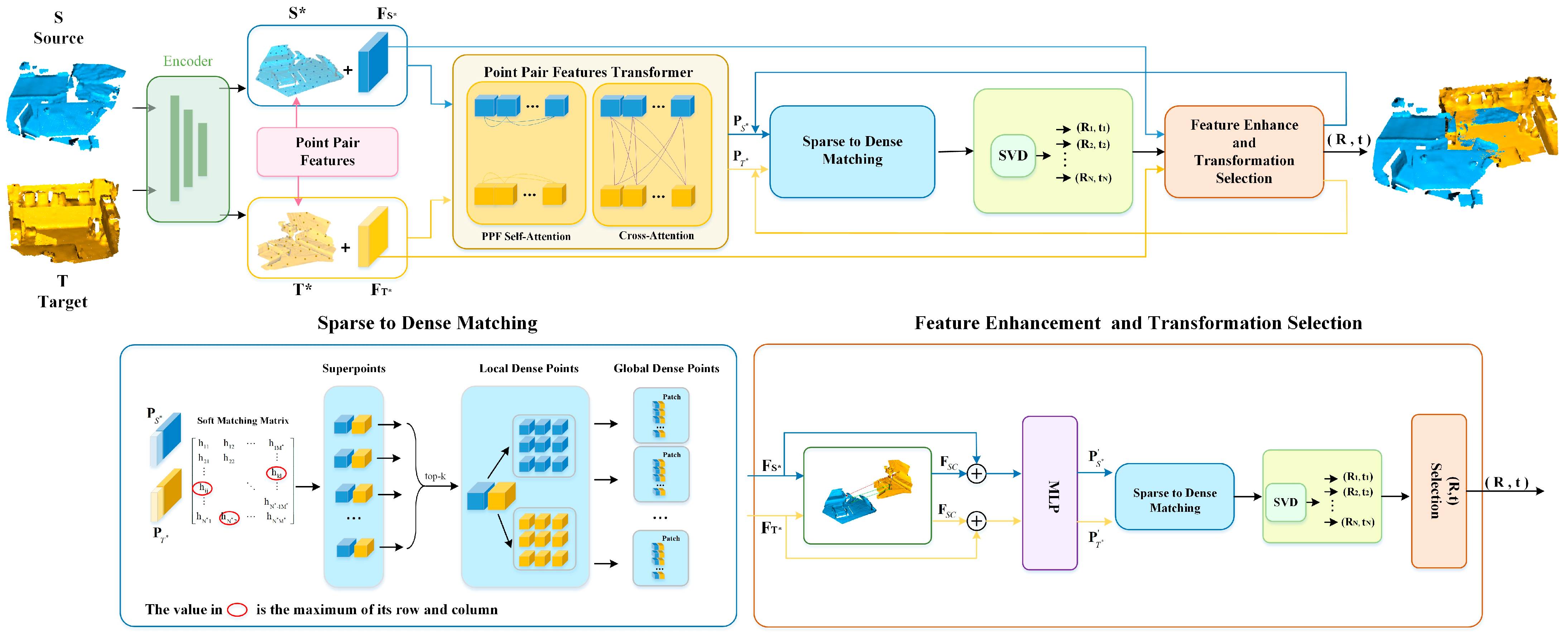
This section illustrates the network architecture as shown in Figure 1. In the encoder stage, the input point clouds and are, respectively, encoded into a set of superpoints with associated features through a KPConv-FPN backbone network, which is then fed into the point pair feature transformer to extract the rotation-invariant hybrid features in both geometric space and feature space. Subsequently, the sparse-to-dense matching module establishes correspondences between superpoints, which are then propagated to local dense points and, further, to global dense points. A set of correspondences is found in each superpoint corresponding patch, and a series of transformation parameters are obtained by utilizing SVD. Finally, spatial consistency is used to enhance the hybrid features, and the enhanced features are repeatedly fed into the sparse-to-dense matching module to rebuild more reliable correspondences and gradually optimize registration, which leads to the final transformation parameters.
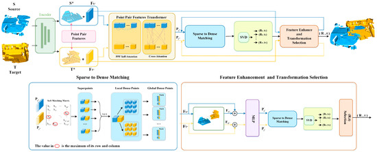
Figure 1.
Network architecture overview.
3.3. Encoder to Superpoint
We use the KPConv-FPN backbone [41,44,49] to aggregate the original point clouds into a much coarser subset of points with their associated features. In the above processing, grid sampling is adopted for downsampling, which can uniformly cover the points in space and make KPConv robust to different densities. Moreover, the learned latent features are enhanced by combining KPConv and a feature pyramid network (FPN), which extract multi-level features from point clouds of different resolutions. Many previous studies have proven that establishing correspondences with coarser points can reduce the number of useless correspondences.
In this paper, we treat the first down-sample points as dense points, and the points with the coarsest resolution are the superpoints. For the convenience of the following illustration, the superpoints corresponding to the source and target clouds are denoted as and , respectively, and their associated learned features are represented by and . Moreover, in order to preserve the information from the original point clouds, we integrate extracted features with point clouds as input features for subsequent processing. The integral features are denoted as and .
3.4. Point Pair Features Transformer Module
Capturing local features is not enough for point cloud registration, with the knowledge that it is necessary to unite the global context. The importance of global context has been shown in many registration tasks [50,51,52]. In order to enrich the contextual information of each input point cloud and exchange the information between the two input point clouds, we proposed a point pair feature [53] transformer (PPF Transformer) module, which contains a point pair feature self-attention (PPF SA) module and a feature-based cross-attention (F CA) module. Previous work has proven that encoding only high-level point features leads to numerous severe outlier matches [35,54]. To address this problem, we encode the internal structure of the point cloud, making it invariant to rigid transformation. PPF self-attention encodes geometric features between the point pairs for each point cloud, and feature-based cross-attention interacts with the feature information between the source point cloud and target point cloud in feature space.
3.4.1. Point Pair Feature Self-Attention
Point pair feature self-attention is designed to learn the rotation-invariant features in both feature space and structure space, which are used to enrich contextual information and measure the feature similarity for each point cloud. Given the input feature matrix, the output contextual feature matrix is updated by the following equation:
where is a three-layer full network; denotes the attention score which represents the similarity between and ; and is computed as follows:
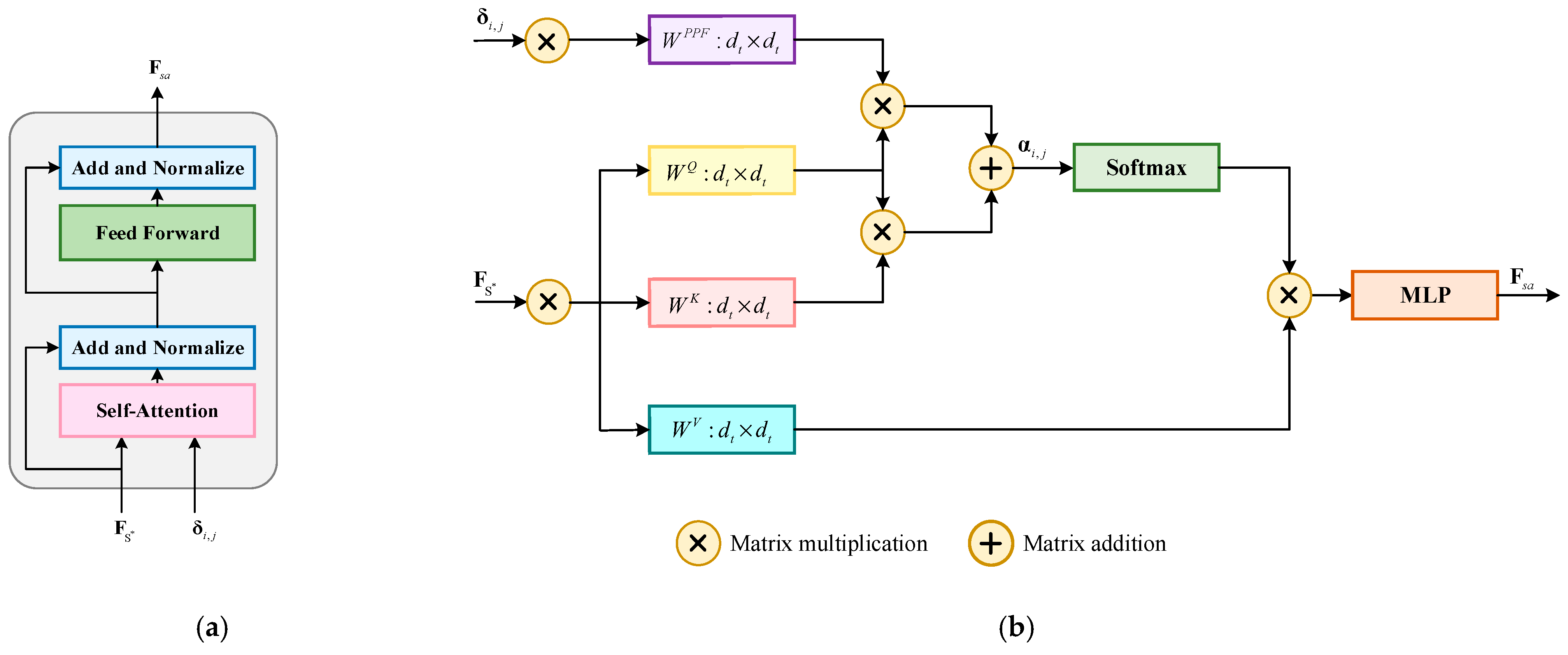
and are the associated features of two superpoints and , respectively; represents the point pair feature between and ; and , , , and denote the learnable weighted matrices for queries, keys, values, and point pair features, respectively. The structure and calculation method of PPF self-attention is shown in Figure 2, whose process is first carrying out a softmax on attention score , then multiplying the matrix obtained from the previous step by the value vector and then via an MLP layer, and finally summing the output result of the liner layer to obtain the final feature. The PPF self-attention features for the point cloud are obtained in the same way.
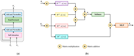
Figure 2.
Illustration of (a) the structure of the PPF self-attention layer and (b) the computation of the feature matrix .
For each superpoint, we construct a patch with the point-to-node strategy [44], and the patch is composed of a series of dense points which are defined as follows:
In order to generate rotation-invariant features, we embed the point pair feature into the attention score . Point pair feature consists of four components, as shown in Figure 3, which are defined as follows:
where and are the normals of superpoints and respectively, which are computed by using the k-nearest neighbors dense points of the superpoints. In Equation (5), is the distance between superpoints and , and denote the angles between the respective normals and the vector of two superpoints, is the angle between the two normals, and and are calculated as follows:

Figure 3.
Point pair feature of the superpoint. The red dots denote superpoints, and the blue dots denote the neighbor’s dense points of the superpoints.
3.4.2. Feature-Based Cross-Attention
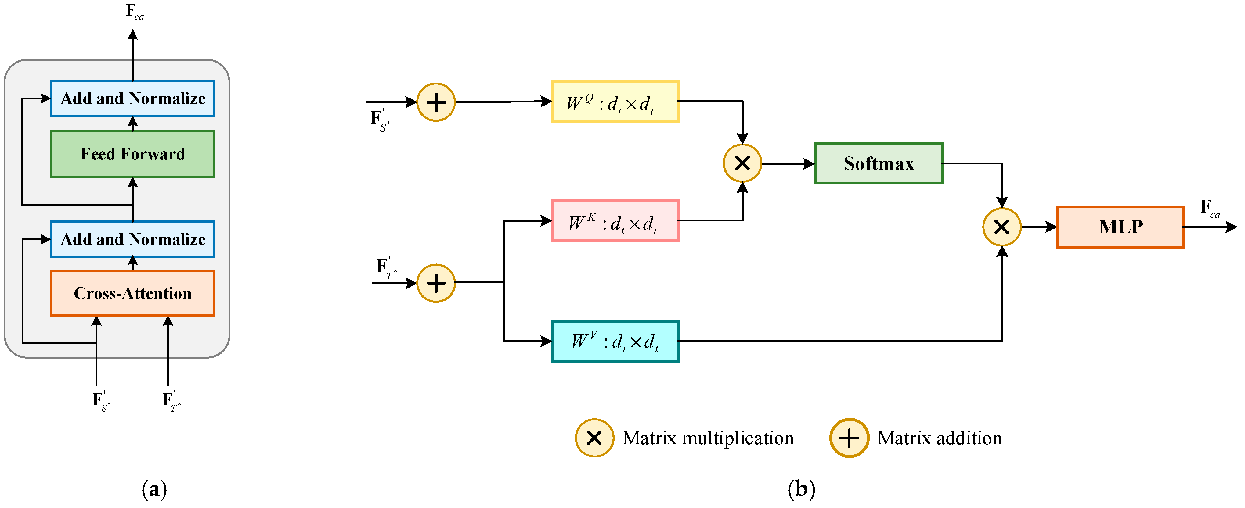
Cross-attention is utilized to exchange the information between two input point clouds, the structure and calculation method of cross-attention is shown in Figure 4. We denote the output feature matrices of the self-attention module for and as and , respectively, which are the input features of the cross-attention module, and the cross-attention features of can be computed as follows:
where is the correlation score between and , which is defined as follows:
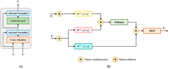
Figure 4.
Illustration of (a) the structure of the cross-attention layer and (b) the computation of the feature matrix .
The cross-attention features of can be computed in the same way, and so far, the information exchange has been completed. Benefiting from the rotation-invariant features encoded by the PPF SA module, the mixed features are rotation-invariant to rigid transformation and contribute to finding the superpoints’ correspondences.
3.5. Sparse-to-Dense Matching
3.5.1. Sparse Matching
Benefiting from the distinctive hybrid features and , we find the superpoints correspondences by utilizing a differentiable optimal transport. The similarity matrix is calculated as follows:
Subsequently, is computed as the augmented matrix of by appending a new row and a new column, as reported in [47], which is filled with a learnable dustbin parameter . Then, a Sinkhorn algorithm [55] is implemented on to calculate the soft matching matrix , and the sparse matching is converted to an optimal transport problem by computing the maximization of . The soft matching score can be obtained by removing the last row and column of . In practical terms, the soft matching score guides the ratio of inliers. For example, when the value is higher, the possibility of this point pair being the correct correspondence is greater. Here, we pick reliable superpoints correspondences based on the strategy with top-k matching scores, where a superpoints correspondence is selected if its matching score is the maximum in both its row and column. However, it is possible for the accuracy of superpoints’ correspondences to be compromised when there are repetitive and textureless structures in the scene. Thus, the proposed method needs to be further strengthened to reduce the mismatching caused by the above-mentioned issues.
3.5.2. Dense Matching
Sparse matching is effective in solving global ambiguity, and the dense matching module is designed to improve robustness at the level of dense points. The matching process propagates the establishment of superpoints’ correspondences to local dense points and, further, to global dense points. The final global correspondences are collected from all local correspondences. Based on the coarse correspondences, we first find the patch-wise correspondences in the same way in which we obtained the superpoints’ correspondences. The difference is that the similarity matrix is computed with the features generated by the backbone. Then we estimate a transformation parameter for each superpoints’ correspondence with their patches in the dense point cloud, generating the local correspondences in each patch. The transformation matrix is solved by the following:
where the soft matching score calculated above is used as the weighting coefficient , and this equation can be solved via SVD. Then, we choose a transformation parameter from to be used in global point matching, with the condition that the patch corresponding to has the highest inlier ratio among all patches.
Here, is the Iverson bracket and is the inlier threshold.
3.6. Progressive Alignment with Spatial Consistency
In this stage, spatial consistency features are learned repeatedly to enhance the distinctiveness of the above-learned features in order to find more reliable superpoints’ correspondences, and the matching results are gradually optimized with the more reliable correspondences. Spatial consistency is the byproduct of rigid transformation, which is determined by the property of isometric isomorphism. We leverage spatial consistency to obtain correct dense correspondences, which depend on the spatial geometric structure between all inlier points not changing with rotation and translation, as shown in Figure 5.
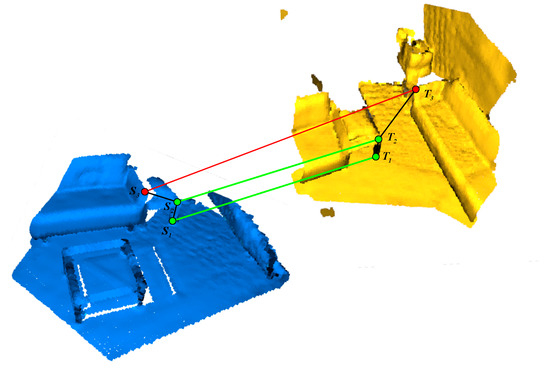
Figure 5.
Illustration of spatial consistency. The green line denotes inlier correspondence, and the red line denotes outlier correspondence.
According to the property of isometric isomorphism, we compute spatial consistency features and feed them into an MLP with 4 hidden layers after normalization; the output is a spatial consistency feature that is used to update the hybrid features via direct addition. Subsequently, we compute the spatial consistency feature with Equation (13), and the same goes for . The hybrid features are updated as shown in Equation (14).
Here, first computed with , and subsequently with computed using Equation (10); is a linear projection function; represents the dot-product similarity [43]; and, denotes the spatial consistency constraint, calculated as follows:
where is used to ensure that is always non-negative, is a distance parameter sensitive to length difference, and denotes the length difference between the segment of two points in point cloud and the segment of two corresponding points in point cloud ; definition of is as follows:
where and are the updated superpoints with the transformation matrix , which is the result of dense matching; and are calculated via Equation (17).
We repeat the operation of feature enhancement to rebuild reliable correspondences from the sparse matching stage, and then we re-estimate the optimal transformation parameters with surviving inliers in the dense matching stage. In fact, the transformation estimated via sparse matching is quite good, but the enhanced features are more distinctive and further improve the accuracy of registration, especially in scenes with many repetitive and textureless structures.
3.7. Loss Functions
In this paper, sparse matching and dense matching directly influence the quality of point cloud registration, so we designed superpoints matching loss and points matching loss to supervise the above two stages, and the total loss function is computed as follows:
In the following description, we take the loss on the source point cloud as an example, and the loss on the target point cloud can be computed in the same way, which will not be repeated later.
3.7.1. Superpoint Loss
We follow [44] and utilize the improved circle loss [56] to supervise the patch-wise feature descriptors for sparse matching in a metric-learning fashion. Here we consider that several patches of superpoints exist in the source point cloud , which have at least one positive patch in the target point cloud . The above patch pairs form the patch set . For each patch , the sets of its positive and negative patches in point cloud are represented as and respectively. Here, a positive patch means that the patch shares a >10% overlap region with patch , while a negative patch means that there is no overlap region. The superpoint matching loss on the point cloud is computed as follows:
where denotes the distance in feature space; is calculated as ; represents the overlap ratio between ; and are the positive and negative weights and are calculated as and , respectively, is a hyper-parameter; and and denotes the positive and negative margins, respectively, which are set to and empirically. The overall superpoint matching loss is .
3.7.2. Point Matching Loss
For point matching loss, we obtain the sets of ground-truth superpoint correspondences and dense correspondences with the ground-truth relative transformation and a matching radius . Here, the set of ground-truth dense correspondences in a pair of patches is denoted as , and those unmatched points of the patch-pairs are represented as and ; and the point matching loss is defined as follows:
4. Experiments and Results
In this section, a series of experiments and comparisons were implemented on several publicly available datasets to analyze the experimental results and evaluate our method. Firstly, we performed comparative experiments on the 3DMatch [29] and 3DLoMatch [54] datasets, and we evaluated the performance with three metrics: IR, FMR, and RR. Subsequently, we checked the effectiveness of our approach on ModelNet [57] and ModelLoNet [54] with another three metrics: RRE, RTE, and RR. Furthermore, we conducted a series of additional comparison experiments on KITTI datasets to verify the validation of our method in large scenes. Finally, extensive ablation studies were conducted to illustrate the validity of the submodules.
The experiments were trained in 40 epochs on 3DMatch, 200 epochs on ModelNet40, and 80 epochs on KITTI with the Adam optimizer and initial learning rates of 0.005, 0.01, and 0.05, respectively. The batch size was set to 1 and the weight decay was set to 1 × 10⁻⁶ in all experiments. The learning rate is exponentially decayed by 0.05 for each epoch on 3DMatch and ModelNet40, and every four epochs on KITTI. We implemented the project on a platform with an Intel i7-11700K CPU and a Geforce RTX 3090 GPU. All programs depended on the environment with Pytorch 1.7.1, Python 3.8, CUDA 11.1, and cuDNN 8.1.0.
4.1. Experiments on 3DMatch and 3DLoMatch
4.1.1. Dataset and Metrics
The 3DMatch dataset is a typical indoor dataset captured by different depth sensors; it contains 62 scenes combining earlier data from RGB-D Scenes and 7 scenes et al., providing great diversity. We divided all scenes into three sets, with 46 scenes, 8 scenes, and 8 scenes, which we used for training, validation, and testing, respectively. Each scene consists of a series of partially overlapped point clouds with their ground-truth transformation. In this paper, we evaluate the proposed approach on 3DMatch and 3DLoMatch datasets, and the difference between 3DMatch and 3DLoMatch is that the overlap of the point cloud pairs in 3DMatch is more than 30%, while in 3DLoMatch it is 10~30%.
We evaluated the performance with reference to [44,54] utilizing three metrics: inlier ratio (IR), feature matching recall (FMR), and registration recall (RR).
IR is computed as the ratio of assumed correspondences, whose residual distance is smaller than a practical value set to through the ground-truth transformation ; the definition is as follows:
FMR is the proportion of point cloud pairs whose IR is larger than a practical threshold (), which is used to measure the potential of success and computed as follows:
where denotes the number of all point cloud pairs.
RR is the most reliable metric since it evaluates the end-to-end performance for registration; it is computed as the proportion of correctly registered point cloud pairs whose transformation error is smaller than a certain threshold (). After applying the estimated transformation, the transformation error can be computed as follows:
And the registration recall is computed as follows:
4.1.2. Registration Results
The registration results of STDRIF were compared with six recent excellent methods: FCGF [30], D3Feat [31], Predator [54], SpinNet [10], REGTR [40], and Geotransformer [44]. We evaluated the performance with the FMR, IR, and RR metrics and reported the results on 3DMatch and 3DLoMatch with 5000, 2500, 1000, 500, and 250 correspondences, as shown in Table 1.

Table 1.
Evaluation results for 3DMatch and 3DLoMatch. The best two performances are highlighted in bold and underlined, respectively.
The evaluation results for 3DMatch and 3DLoMatch are exhibited separately on the left and right sides of Table 1, respectively. With the FMR metric, the performance was close to Geotransformer on 3DMatch, and it showed a better improvement on 3DLoMatch, verifying the validity of the submodules designed for finding correspondences. With the IR metric, the performance was superior to that of other methods, demonstrating the more reliable correspondences produced. RR was the most reliable and intuitive metric used to evaluate the performance of final registration, and the evaluation result directly proves the effectiveness of our approach. Overall, our approach performed best on 3DMatch, with close results compared to Geotransformer and significant improvements over other comparison methods. The performance on 3DLoMatch was still strongly competitive. The evaluation results verify the robustness of our method.
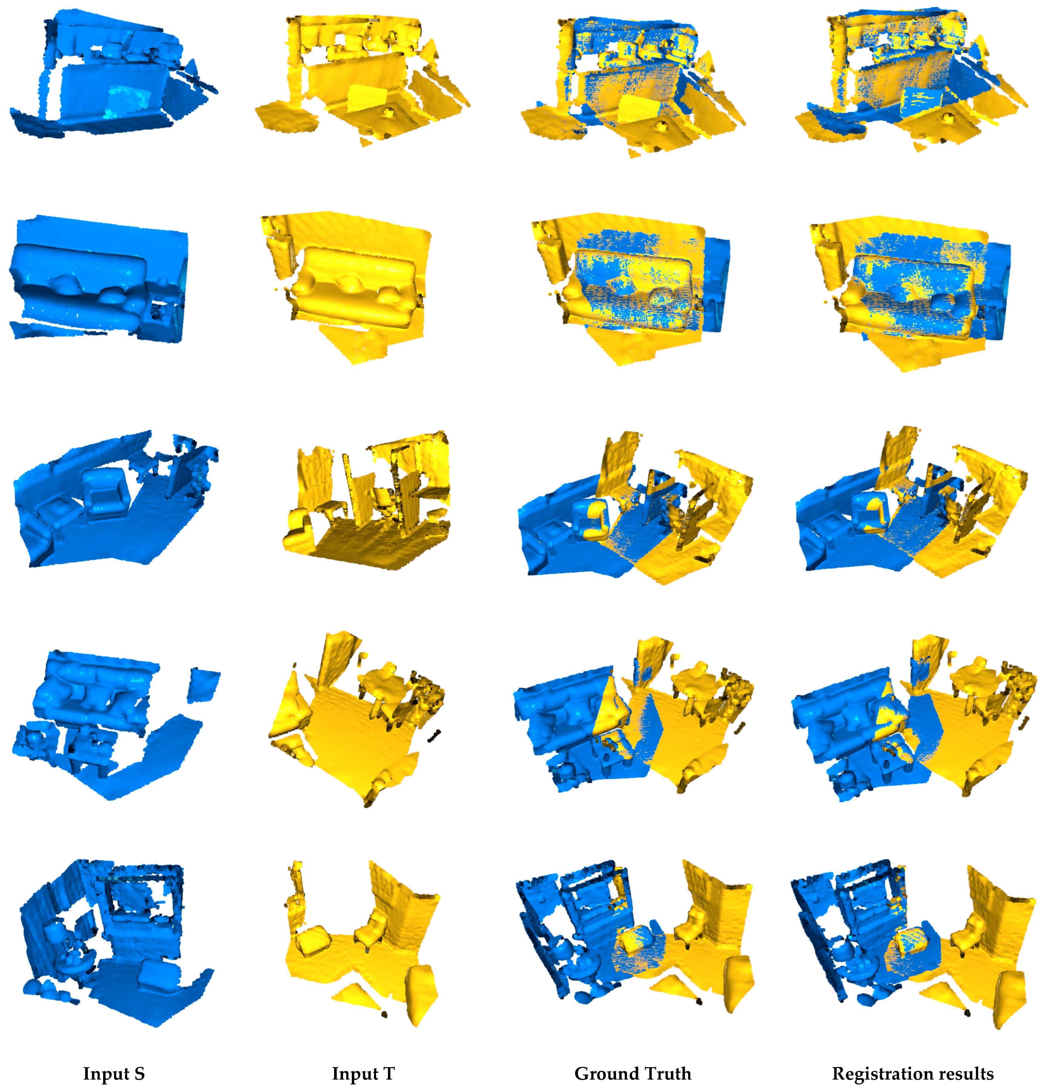
In order to show the reliability of our approach intuitively, a visualization of the registration results on 3DMatch and 3DLoMatch with 5000 correspondences is displayed in Figure 6, which contains five examples represented in five separate lines. In each example, the first two columns denote the source and target point clouds, respectively. The third column denotes the ground truth, and the last column denotes the registration result. From the comparison of the registration results and ground truth, it can be seen that our method performs satisfactorily, especially in low-overlap scenes.
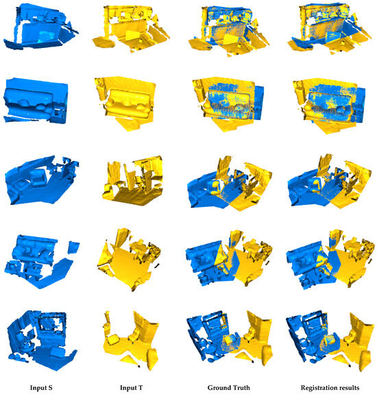
Figure 6.
Visualization of five registration result examples on 3DMatch and 3DLoMatch. In each example, the source point cloud S, target point cloud T, ground truth, and registration result are represented from left to right. The first two rows display the results of high-overlap registration, and the last three rows display the results of low-overlap registration.
4.2. Experiments on ModelNet40
4.2.1. Dataset and Metrics
ModelNet40 contains 40 different categories of CAD models, each of which consists of training and test data collected from these CAD models. We used the processed dataset as described in [54], among which are 5112 models for training, 1202 models for validation, and 1266 models for testing. We performed the experiments on both ModelNet and ModelLoNet, where the overlap of point cloud pairs in ModelNet was ~70%, while in ModelLoNet it was ~50%. On ModelNet40, we reported the relative rotation error (RRE), the relative translation error (RTE), and the chamfer distance (CD) to evaluate our method [32].
RRE is the geodesic and Euclidean distance between the estimated and ground-truth rotation matrices, which measures the differences between the predicted and ground-truth rotation matrix, computed as follows:
RTE is the Euclidean distance between the estimated and ground-truth translation vectors, which measures the differences between the predicted and ground-truth translation matrix, which is computed as follows:
CD is the average nearest squared distance between the predicted and ground-truth point clouds, which measures the similarity between the predicted and ground-truth point clouds, defined as follows:
4.2.2. Registration Results
We compared the registration results of our method with those of five other methods on ModelNet40: PointNetLK [15], DCP [35], RPM-Net [32], Predator [54], and REGTR [40]. Three metrics (RRE, RTE, and CD) were used to measure the performance of ModelNet and ModelLoNet, as shown in Table 2. The left and right sides of Table 2 present the evaluation results for ModelNet and ModelLoNet, respectively. According to the evaluation on ModelNet, although the result with RTE was inferior to that of REGTR, it can be seen that STDRIF performed better than the other comparison methods with the RTE and CD metrics in high-overlap and low-overlap models.
Table 2.
The registration results on ModelNet and ModelLoNet. The best two performances are highlighted in bold and underlined, respectively.
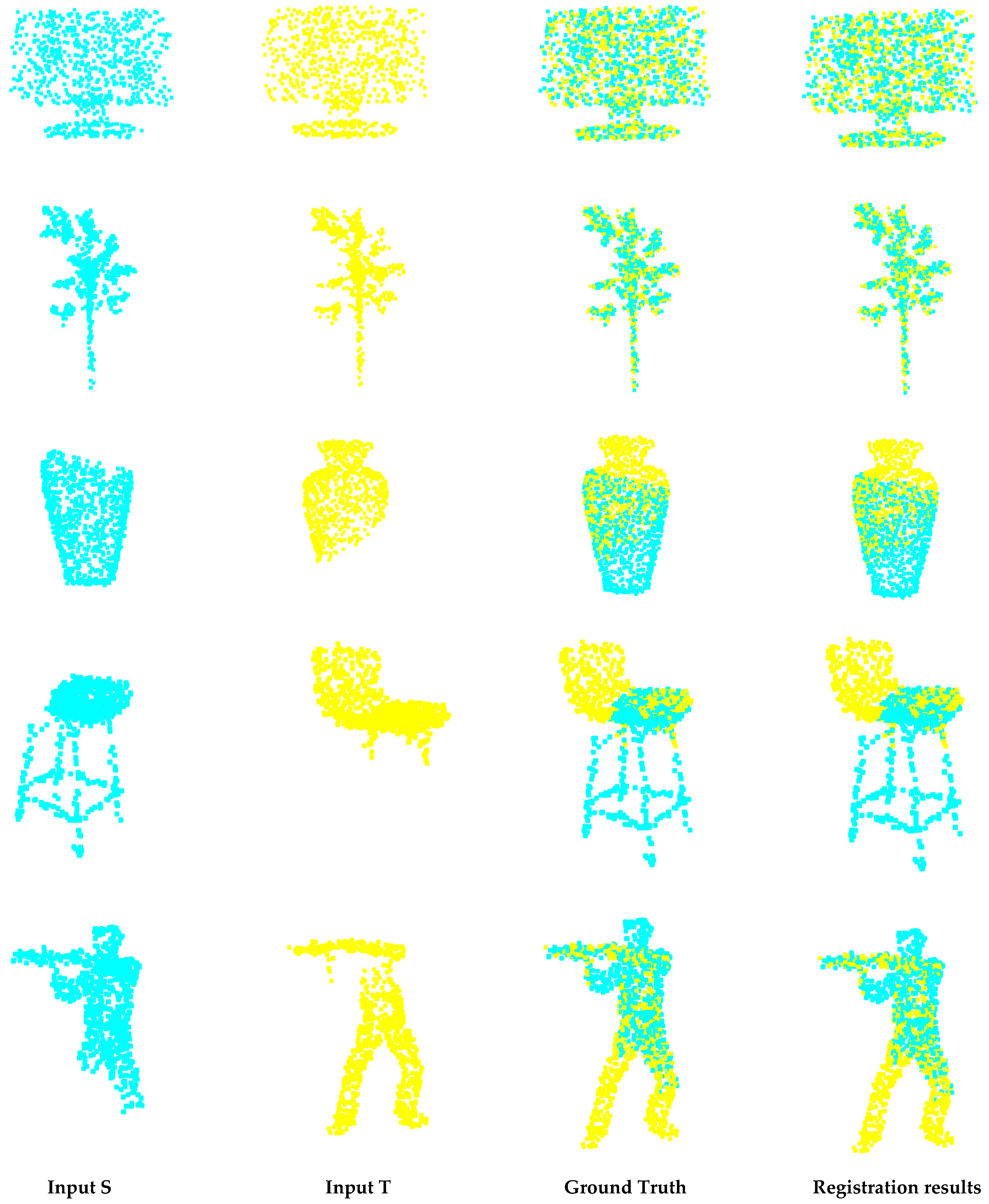
Figure 7 presents the registration results on ModelNet and ModelLoNet. Figure 8 displays the results of a comparison experiment between our method and Predator on ModelNet with different overlap ratios using the RRE and RTE metrics. In Figure 7, it can be seen that the registration results are close to the ground truth, which intuitively demonstrates the effectiveness of the proposed method. Figure 8 shows that the registration performance became worse with the decline in the overlap ratio; however, the results of our method were always superior to those of Predator with RRE and RTEe, which further proves that our method is competitive even for low-overlap registration.
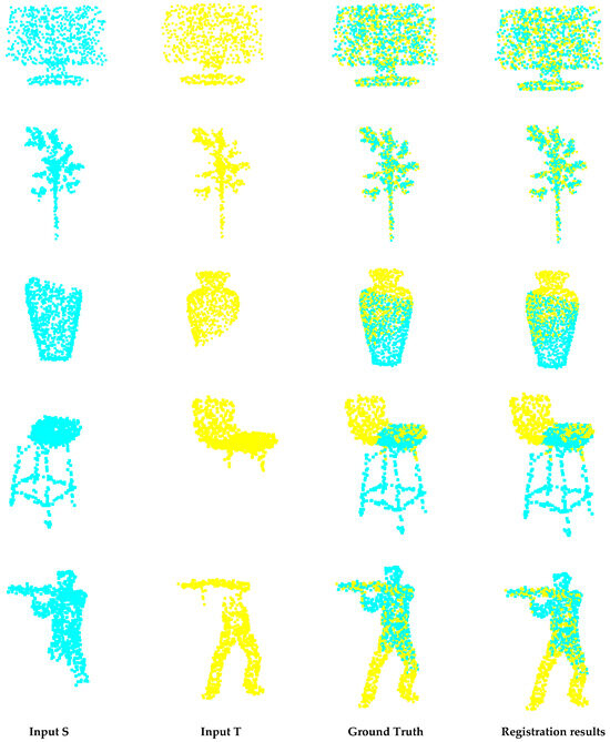
Figure 7.
Visualization of registration results on ModelNet and ModelLoNet. In each example, the input source point cloud S, input target point cloud T, ground truth, and registration result are represented from left to right. The first two rows display the results on ModelNet, and the last three rows display the results on ModelLoNet.
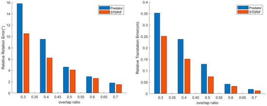
Figure 8.
Comparison performance of STDRIF and Predator on ModelNet40 with different overlap ratios.
4.3. Experiments on KITTI
4.3.1. Dataset and Metrics
OdometryKITTI [30,31,44,54] includes 11 sequences of outdoor driving scenarios scanned using Velodyne laser LIDAR, among which sequences 0–5 are for training, sequences 6–7 are for validation, and sequences 8–10 are for testing. We used the method of [44,54] to refine the ground truth pose with ICP, and we evaluated our method with the point cloud pairs that are up to 10 m away from one another. The evaluation metrics used on KITTI are RRE, RTE, and RR; these three metrics have already been introduced in Section 4.1.1 and Section 4.2.1 and they will not be repeated here.
4.3.2. Registration Results
A comparison of the registration results is shown in Table 3, and the comparison methods included five recent outstanding methods: 3DFeat-Net [58], FCGF [30], D3Feat [32], Predator [54], and Geotransformer [44]. With the RTE and RR metrics, we obtained the same performance as with Predator and Geotransformer. With RRE, the performance of our method was slightly inferior to that of Geotransformer. Overall, our method is still competitive in large scenes.
Table 3.
The registration results on KITTI. The best two performances are highlighted in bold and underlined, respectively.
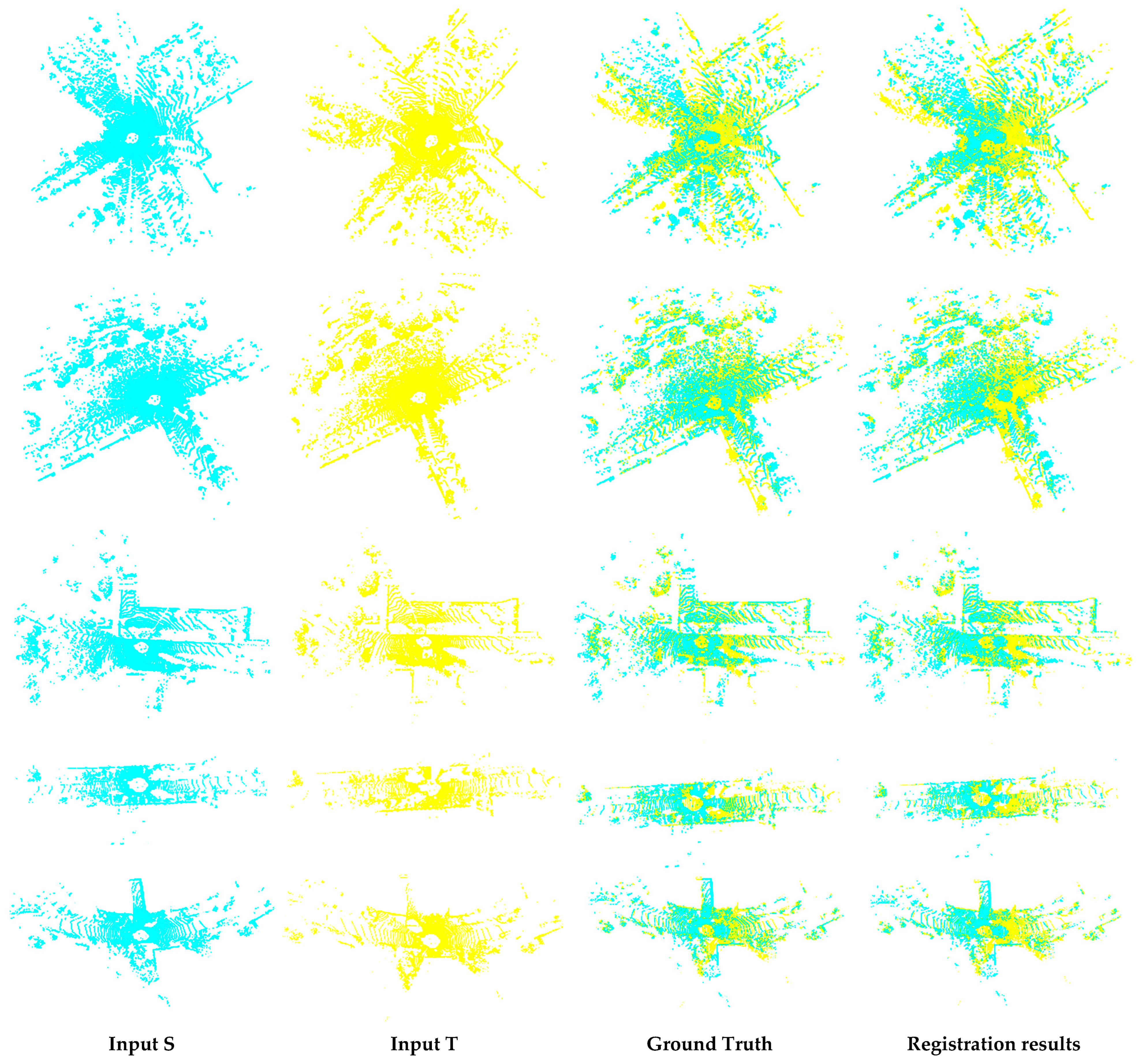
Figure 9 displays the five examples of visualization results of registration on odometryKITTI, which intuitively shows the reliability of our approach. In Figure 8, each line exhibits an example of the registration result. In each example, the first two columns denote the source and target point clouds, respectively. The third column denotes the ground truth, and the last column denotes the registration result. From the comparison of the registration results and ground truth, it can be seen that the proposed method performs satisfactorily in large scenes.
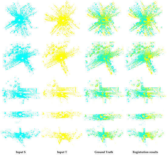
Figure 9.
Visualization of registration results on KITTI. In each example, the input source point cloud S, input target point cloud T, ground truth, and registration result are represented from left to right.
4.4. Ablation Studies
Extensive ablation studies were conducted by applying one proposed submodule to the baseline at each time. Since the registration results of our method were close to those reported in [40], we chose [54] as the baseline to present the corresponding contribution of each submodule. Table 4 shows the extensive results on 3DMatch and 3DLoMatch. Our method benefits from three key components: PPF Transformer (PPF), sparse-to-dense matching (STD), and progressive alignment (PA). It can be seen that FMR, IR, and RR improved with each component used in the baseline, and the performance was better when submodules were used in superposition. The method using three submodules on the 3DMatch and 3DLoMatch datasets led to an increase of 3% and 3.7% in the RR metric, respectively, compared to the baseline with no submodules. Furthermore, using three submodules on the 3DMatch and 3DLoMatch datasets, the RR increased more obviously on the 3DLoMatch, which demonstrates that our approach is more competitive for low-overlap point cloud registration tasks.
Table 4.
Ablation study for each submodule, tested with 5000 correspondences. The best two performances are highlighted in bold and underlined, respectively. The √ and x indicate whether or not the module is in use, respectively.
5. Discussion
5.1. Performance and Effectiveness Analysis
In this study, several experiments were implemented on the 3DMatch, ModelNet40, and KITTI datasets. For all datasets, in order to show the excellent performance of our method, we reported the evaluation results with respective metrics and displayed the visualization of the registration results in the Section 4.1, Section 4.2 and Section 4.3. The evaluation results verify that the registration performance of our approach is superior to that of other recent excellent methods, even in large scenes, and the visualization of the registration results demonstrates the practicability and feasibility of our method. In the Section 4.4, ablation studies were conducted to explore the influence of each submodule with the FMR, IR, and RR metrics on 3DMatch. The value of the metrics increased with each submodule applied to the baseline, demonstrating the validity of the proposed submodules. Ablation studies on 3DLoMatch showed more significant performance improvements than on 3DMatch, demonstrating that our approach remains competitive in low-overlap scenes.
5.2. Limitations and Future Improvement Directions
A series of experiments have shown that STDRIF performs excellently with high accuracy and robustness, especially for low-overlap registration tasks. However, the limitations of our approach must be discussed below for the improvement of future work. In the above illustration, the PPF Transformer module was leveraged to learn rotation-invariant features. We focused on the point pair features in the self-attention stage to enrich contextual information, but we neglected the awareness of spatial positions when exchanging and aggregating information in the cross-attention stage. Moreover, we followed the method of [44] to downsample the input point clouds with the grid sampling method, which may lead to numerous superpoints and cause an increase in the calculation cost. The limitations mentioned above will be improved upon in future work. Except for the above details in need of improvement, we hope our method can cover a wider range of applications, such as non-rigid registration, cross-modality registration, etc.
6. Conclusions
In this paper, we introduced a point cloud registration network based on rotation-invariant features with a sparse-to-dense matching strategy, and the registration results benefit from three key submodules: PPF, STD, and PA. The PPF transformer module embeds point pair features into the transformer, which learns the distinctive hybrid features that make it invariant to rigid transformation. Sparse-to-dense matching establishes reliable correspondences from sparse to dense. The progressive alignment module further optimizes the registration by finding higher inlier ratio superpoints correspondences based on consistency. We conducted several experiments on the 3DMatch, ModelNet40, and KITTI datasets, and we showed the visualization and evaluation of the registration results. We further conducted ablation studies on the 3DMatch dataset and demonstrated the effectiveness of the three key submodules. All of the experimental results verify the excellent performance of our method, especially for low-overlap registration tasks and in large scenes. Finally, we discussed the limitations and future improvement directions. The remaining issues will be addressed in our future work for more robust and applicable point cloud registration.
Author Contributions
Conceptualization, T.M.; validation, T.M. and G.H.; formal analysis, T.M., Y.C. and H.R.; investigation, T.M., Y.C. and H.R.; original draft preparation, T.M.; review and editing, T.M., Y.C., H.R. and G.H.; visualization, T.M.; funding acquisition, G.H. All authors have read and agreed to the published version of the manuscript.
Funding
This work was partially funded by the Department of Science and Technology of Jilin Province under Grant 20210201132GX.
Data Availability Statement
All datasets used in this work are available from the corresponding author upon request.
Conflicts of Interest
The authors declare no conflicts of interest.
References
- Eldefrawy, M.; King, S.A.; Starek, M. Partial Scene Reconstruction for Close Range Photogrammetry Using Deep Learning Pipeline for Region Masking. Remote Sens. 2022, 14, 3199. [Google Scholar] [CrossRef]
- Dubé, R.; Gollub, M.G.; Sommer, H.; Gilitschenski, I.; Siegwart, R.; Cadena, C.; Nieto, J.I. Incremental-Segment-Based Localization in 3-D Point Clouds. IEEE Robot. Autom. Lett. 2018, 3, 1832–1839. [Google Scholar] [CrossRef]
- Chua, C.-S.; Jarvis, R. Point Signatures: A New Representation for 3D Object Recognition. Int. J. Comput. Vis. 1997, 25, 63–85. [Google Scholar] [CrossRef]
- Qi, C.R.; Su, H.; Mo, K.; Guibas, L.J. PointNet: Deep Learning on Point Sets for 3D Classification and Segmentation. In Proceedings of the 2017 IEEE Conference on Computer Vision and Pattern Recognition, CVPR 2017, Honolulu, HI, USA, 21–26 July 2017; IEEE Computer Society: Washington, DC, USA, 2017; pp. 77–85. [Google Scholar]
- Ali, S.A.; Kahraman, K.; Reis, G. RPSRNet: End-to-End Trainable Rigid Point Set Registration Network using Barnes-Hut 2D-Tree Representation. arXiv 2021, arXiv:2104.05328. [Google Scholar]
- Noh, J.; Lee, S.; Ham, B. HVPR: Hybrid Voxel-Point Representation for Single-stage 3D Object Detectio. arXiv 2021, arXiv:2104.00902. [Google Scholar]
- Besl, P.J.; McKay, N.D. Method for registration of 3-D shapes. In Proceedings of the Sensor Fusion IV: Control Paradigms and Data Structures, Boston, MA, USA, 12–15 November 1991; SPIE: Bellingham, WA, USA, 1992; Volume 1611, pp. 586–606. [Google Scholar]
- Abdi, H. Singular value decomposition (SVD) and generalized singular value decomposition. Encycl. Meas. Stat. 2007, 907, 44. [Google Scholar]
- Fischler, M.A.; Bolles, R.C. Random sample consensus: A paradigm for model fitting with applications to image analysis and automated cartography. Commun. ACM 1981, 24, 381–395. [Google Scholar] [CrossRef]
- Ao, S.; Hu, Q.; Yang, B.; Markham, A.; Guo, Y. SpinNet: Learning a General Surface Descriptor for 3D Point Cloud Registration. In Proceedings of the IEEE Conference on Computer Vision and Pattern Recognition, CVPR 2021, Virtual, 19–25 June 2021; IEEE: New York, NY, USA, 2021; pp. 11753–11762. [Google Scholar]
- Deng, H.; Birdal, T.; Ilic, S. Ppfnet: Global context aware local features for robust 3d point matching. In Proceedings of the IEEE Conference on Computer Vision and Pattern Recognition, Salt Lake City, UT, USA, 18–23 June 2018; pp. 195–205. [Google Scholar]
- Li, J.; Zhang, C.; Xu, Z.; Zhou, H.; Zhang, C. Iterative distance-aware similarity matrix convolution with mutual-supervised point elimination for efficient point cloud registration. In Proceedings of the 16th European Conference on Computer Vision, Glasgow, UK, 23–28 August 2020; Springer: Cham, Switzerland, 2020; pp. 378–394. [Google Scholar]
- Chen, Z.; Yang, F.; Tao, W. Detarnet: Decoupling translation and rotation by siamese network for point cloud registration. In Proceedings of the AAAI Conference on Artificial Intelligence, Virtually, 22 February–1 March 2022; pp. 401–409. [Google Scholar]
- Gojcic, Z.; Zhou, C.; Wegner, J.D.; Wieser, A. The Perfect Match: 3D Point Cloud Matching with Smoothed Densities. In Proceedings of the IEEE Conference on Computer Vision and Pattern Recognition, CVPR 2019, Long Beach, CA, USA, 16–20 June 2019; IEEE: New York, NY, USA, 2019; pp. 5545–5554. [Google Scholar]
- Aoki, Y.; Goforth, H.; Srivatsan, R.A.; Lucey, S. PointNetLK: Robust&Efficient Point Cloud Registration Using PointNet. In Proceedings of the IEEE Conference on Computer Vision and Pattern Recognition, CVPR 2019, Long Beach, CA, USA, 16–20 June 2019; IEEE: New York, NY, USA, 2019; pp. 7163–7172. [Google Scholar]
- Wang, Y.; Solomon, J.M. Prnet: Self-supervised learning for partial-to-partial registration. arXiv 2019, arXiv:1910.12240. [Google Scholar]
- Yang, Z.; Pan, J.Z.; Luo, L.; Zhou, X.; Grauman, K.; Huang, Q. Extreme Relative Pose Estimation for RGB-D Scans via Scene Completion. In Proceedings of the IEEE Conference on Computer Vision and Pattern Recognition, CVPR 2019, Long Beach, CA, USA, 16–20 June 2019; IEEE: New York, NY, USA, 2019; pp. 4531–4540. [Google Scholar]
- Elbaz, G.; Avraham, T.; Fischer, A. 3D Point Cloud Registration for Localization Using a Deep Neural Network Auto-Encoder. In Proceedings of the 2017 IEEE Conference on Computer Vision and Pattern Recognition, CVPR 2017, Honolulu, HI, USA, 21–26 July 2017; IEEE Computer Society: Washington, DC, USA, 2017; pp. 4631–4640. [Google Scholar]
- Choy, C.; Dong, W.; Koltun, V. Deep global registration. In Proceedings of the 2020 IEEE/CVF Conference on Computer Vision and Pattern Recognition, CVPR 2020, Seattle, WA, USA, 13–19 June 2020; IEEE: New York, NY, USA, 2020; pp. 2514–2523. [Google Scholar]
- Yang, J.; Li, H.; Campbell, D.; Jia, Y. Go-ICP: A Globally Optimal Solution to 3D ICP Point-Set Registration. IEEE Trans. Pattern Anal. Mach. Intell. 2016, 38, 2241–2254. [Google Scholar] [CrossRef] [PubMed]
- Segal, A.; Hhnel, D.; Thrun, S. Generalized-ICP. In Robotics: Science and Systems V; IEEE: Seattle, WA, USA, 2019; p. 435. [Google Scholar]
- Parkison, S.A.; Gan, L.; Jadidi, M.G.; Eustice, R.M. Semantic Iterative Closest Point through Expectation-Maximization. In Proceedings of the British Machine Vision Conference 2018, BMVC 2018, Newcastle, UK, 3–6 September 2018; BMVA Press: Durham, UK, 2018; p. 280. [Google Scholar]
- Biber, P.; Straßer, W. The normal distributions transform: A new approach to laser scan matching. In Proceedings of the 2003 IEEE/RSJ International Conference on Intelligent Robots and Systems, Las Vegas, NV, USA, 27 October–1 November 2003; IEEE: New York, NY, USA, 2003; pp. 2743–2748. [Google Scholar]
- Rusu, R.B.; Blodow, N.; Beetz, M. Fast point feature histograms (FPFH) for 3D registration. In Proceedings of the 2009 IEEE International Conference on Robotics and Automation, Kobe, Japan, 12–17 May 2009; IEEE: Kobe, Japan, 2009; pp. 3212–3217. [Google Scholar]
- Aiger, D.; Mitra, N.J.; Cohen-Or, D. 4-points congruent sets for robust pairwise surface registration. ACM Trans. Graph. 2008, 27, 1–10. [Google Scholar] [CrossRef]
- Tombari, F.; Salti, S.; Di Stefano, L. Unique signatures of histograms for local surface description. In Proceedings of the 11th European Conference on Computer Vision, Heraklion, Greece, 5–11 September 2010; Springer: Berlin/Heidelberg, Germany, 2010; pp. 356–369. [Google Scholar]
- Jian, B.; Vemuri, B.C. Robust Point Set Registration Using Gaussian Mixture Models. IEEE Trans. Pattern Anal. Mach. Intell. 2011, 33, 1633–1645. [Google Scholar] [CrossRef] [PubMed]
- Eckart, B.; Kim, K.; Kautz, J. HGMR: Hierarchical Gaussian Mixtures for Adaptive 3D Registration. In Proceedings of the Computer Vision—ECCV 2018—15th European Conference, Munich, Germany, 8–14 September 2018; Ferrari, V., Hebert, M., Sminchisescu, C., Weiss, Y., Eds.; Proceedings, Part XV. Springer: Berlin/Heidelberg, Germany, 2018; Volume 11219, pp. 730–746. [Google Scholar]
- Zeng, A.; Song, S.; Nießner, M.; Fisher, M.; Xiao, J.; Funkhouser, T.A. 3DMatch: Learning Local Geometric Descriptors from RGB-D Reconstructions. In Proceedings of the 2017 IEEE Conference on Computer Vision and Pattern Recognition, CVPR 2017, Honolulu, HI, USA, 21–26 July 2017; IEEE Computer Society: Washington, DC, USA, 2017; pp. 199–208. [Google Scholar]
- Choy, C.B.; Park, J.; Koltun, V. Fully Convolutional Geometric Features. In Proceedings of the 2019 IEEE/CVF International Conference on Computer Vision, ICCV 2019, Seoul, Republic of Korea, 27 October–2 November 2019; IEEE: New York, NY, USA, 2019; pp. 8957–8965. [Google Scholar]
- Bai, X.; Luo, Z.; Zhou, L.; Fu, H.; Quan, L.; Tai, C.-L. D3Feat: Joint Learning of Dense Detection and Description of 3D Local Features. In Proceedings of the 2020 IEEE/CVF Conference on Computer Vision and Pattern Recognition, CVPR 2020, Seattle, WA, USA, 13–19 June 2020; IEEE: New York, NY, USA, 2020; pp. 6358–6366. [Google Scholar]
- Yew, Z.J.; Lee, G.H. Rpm-net: Robust point matching using learned features. In Proceedings of the IEEE/CVF Conference on Computer Vision and Pattern Recognition, Seattle, WA, USA, 13–19 June 2020; pp. 11824–11833. [Google Scholar]
- Huang, X.; Mei, G.; Zhang, J. Feature-metric registration: A fast semi-supervised approach for robust point cloud registration without correspondences. In Proceedings of the IEEE/CVF Conference on Computer Vision and Pattern Recognition, Seattle, WA, USA, 13–19 June 2020; pp. 11366–11374. [Google Scholar]
- Vaswani, A.; Shazeer, N.; Parmar, N.; Uszkoreit, J.; Jones, L.; Gomez, A.N.; Kaiser, L.; Polosukhin, I. Attention is All you Need. In Proceedings of the Advances in Neural Information Processing Systems 30: Annual Conference on Neural Information Processing Systems 2017, Long Beach, CA, USA, 4–9 December 2017; pp. 5998–6008. [Google Scholar]
- Wang, Y.; Solomon, J.M. Deep closest point: Learning representations for point cloud registration. In Proceedings of the IEEE/CVF International Conference on Computer Vision, Seoul, Republic of Korea, 27 October–2 November 2019; pp. 3523–3532. [Google Scholar]
- Qi, C.R.; Yi, L.; Su, H.; Guibas, L.J. Pointnet++: Deep hierarchical feature learning on point sets in a metric space. In Advances in neural Information Processing Systems; Morgan Kaufmann Publishers Inc.: San Francisco, CA, USA, 2017; p. 30. [Google Scholar]
- Wang, Y.; Sun, Y.; Liu, Z.; Sarma, S.E.; Bronstein, M.M.; Solomon, J.M. Dynamic Graph CNN for Learning on Point Clouds. ACM Trans. Graph. 2019, 38, 1–12. [Google Scholar] [CrossRef]
- Kabsch, W. A solution for the best rotation to relate two sets of vectors. Acta Crystallogr. Sect. A Cryst.Phys.Diffr. Theor. Gen. Crystallogr. 1976, 32, 922–923. [Google Scholar] [CrossRef]
- Fu, K.; Liu, S.; Luo, X.; Wang, M. Robust point cloud registration framework based on deep graph matching. In Proceedings of the IEEE/CVF Conference on Computer Vision and Pattern Recognition, New Orleans, LA, USA, 18–24 June 2021; pp. 8893–8902. [Google Scholar]
- Yew, Z.J.; Lee, G.H. REGTR: End-to-end Point Cloud Correspondences with Transformers. In Proceedings of the IEEE/CVF Conference on Computer Vision and Pattern Recognition, CVPR 2022, New Orleans, LA, USA, 18–24 June 2022; IEEE: New York, NY, USA, 2022; pp. 6667–6676. [Google Scholar]
- Thomas, H.; Qi, C.R.; Deschaud, J.E.; Marcotegui, B.; Goulette, F.; Guibas, L.J. Kpconv: Flexible and deformable convolution for point clouds. In Proceedings of the IEEE/CVF International Conference on Computer Vision, Seoul, Republic of Korea, 27 October–2 November 2019; pp. 6411–6420. [Google Scholar]
- Wang, X.; Yuan, Y. GCMTN: Low-Overlap Point Cloud Registration Network Combining Dense Graph Convolution and Multilevel Interactive Transformer. Remote Sens. 2023, 15, 3908. [Google Scholar] [CrossRef]
- Bai, X.; Luo, Z.; Zhou, L.; Chen, H.; Li, L.; Hu, Z.; Fu, H.; Tai, C.L. Pointdsc: Robust point cloud registration using deep spatial consistency. In Proceedings of the IEEE/CVF Conference on Computer Vision and Pattern Recognition, Nashville, TN, USA, 20–25 June 2021; pp. 15859–15869. [Google Scholar]
- Qin, Z.; Yu, H.; Wang, C.; Guo, Y.; Peng, Y.; Xu, K. Geometric Transformer for Fast and Robust Point Cloud Registration. In Proceedings of the IEEE/CVF Conference on Computer Vision and Pattern Recognition, CVPR 2022, New Orleans, LA, USA, 18–24 June 2022; IEEE: New York, NY, USA, 2022; pp. 11133–11142. [Google Scholar]
- Yu, H.; Qin, Z.; Hou, J.; Mahdi, S.; Li, D.; Benjamin, B.; Slobodan, I. Rotation-Invariant Transformer for Point Cloud Matching. arXiv 2023, arXiv:2303.08231. [Google Scholar]
- Taewon, M.; Chonghyuk, S.; Eunseok, K.; Inwook, S. Distinctiveness oriented positional equilibrium for point cloud registration. In Proceedings of the IEEE/CVF Conference on Computer Vision, Montreal, Canada, 17 October–27 October 2021; pp. 5490–5498. [Google Scholar]
- Yang, F.; Guo, L.; Chen, Z.; Tao, W. One-inlier is first: Towards efficient position encoding for point cloud registration. In Proceedings of the Advances in Neural Information Processing Systems, New Orleans, LA, USA, 28 November–9 December 2022; pp. 6982–6995. [Google Scholar]
- Li, Y.; Harada, T. Lepard: Learning partial point cloud matching in rigid and deformable scenes. In Proceedings of the IEEE/CVF conference on Computer Vision and Pattern Recognition, CVPR 2022, New Orleans, LA, USA, 18–24 June 2022; IEEE: New York, NY, USA, 2022; pp. 5554–5564. [Google Scholar]
- Lin, T.Y.; Dollar, P.; Girshick, R.; He, K.; Hariharan, B.; Belongie, S. Feature Pyramid Networks for Object Detection. In Proceedings of the IEEE Conference on Computer Vision and Pattern Recognition, CVPR 2021, Virtual, 19–25 June 2021; IEEE: New York, NY, USA, 2021; pp. 2117–2125. [Google Scholar]
- Dosovitskiy, A.; Beyer, L.; Kolesnikov, A.; Weissenborn, D.; Houlsby, N. An image is worth 16 × 16 words: Transformers for image recognition at scale. arXiv 2010, arXiv:2010.11929. [Google Scholar]
- Sun, J.; Shen, Z.; Wang, Y.; Bao, H.; Zhou, X. LoFTR: Detector-Free Local Feature Matching with Transformers. In Proceedings of the IEEE Conference on Computer Vision and Pattern Recognition, CVPR 2021, Virtual, 19–25 June 2021; IEEE: New York, NY, USA, 2021; pp. 4267–4276. [Google Scholar]
- Yu, H.; Li, F.; Saleh, M.; Busam, B.; Ilic, S. Cofinet: Reliable coarse-to-fine correspondences for robust pointcloud registration. Adv. Neural Inf. Process. Syst. 2021, 34, 23872–23884. [Google Scholar]
- Drost, B.; Ulrich, M.; Navab, N.; Ilic, S. Model globally, match locally: Efficient and robust 3D object recognition. In Proceedings of the 2010 IEEE Computer Society Conference on Computer Vision and Pattern Recognition, San Francisco, CA, USA, 13–18 June 2010; IEEE: San Francisco, CA, USA, 2010; pp. 998–1005. [Google Scholar]
- Huang, S.; Gojcic, Z.; Usvyatsov, M.; Wieser, A.; Schindler, K. Predator: Registration of 3D Point Clouds with Low Overlap. In Proceedings of the IEEE Conference on Computer Vision and Pattern Recognition, CVPR 2021, Virtual, 19–25 June 2021; IEEE: New York, NY, USA, 2021; pp. 8922–8931. [Google Scholar]
- Sinkhorn, R.; Knopp, P. Concerning nonnegative matrices and doubly stochastic matrices. Pac. J. Math. 1967, 21, 343–348. [Google Scholar] [CrossRef]
- Sun, Y.; Cheng, C.; Zhang, Y.; Zhang, C.; Zheng, L.; Wang, Z.; Wei, Y. Circle loss: A unified perspective of pair similarity optimization. In Proceedings of the 2020 IEEE/CVF Conference on Computer Vision and Pattern Recognition, CVPR 2020, Seattle, WA, USA, 13–19 June 2020; IEEE: New York, NY, USA, 2020; pp. 6398–6407. [Google Scholar]
- Wu, Z.; Song, S.; Khosla, A.; Yu, F.; Zhang, L.; Tang, X.; Xiao, J. 3d shapenets: A deep representation for volumetric shapes. In Proceedings of the IEEE Conference on Computer Vision and Pattern Recognition, Boston, MA, USA, 7–12 June 2015; pp. 1912–1920. [Google Scholar]
- Yew, Z.; Lee, G. 3dfeat-net: Weakly supervised local 3d features for point cloud registration. In Proceedings of the European conference on computer vision, ECCV 2018, Munich, Germany, 8–14 September 2018; pp. 607–623. [Google Scholar]


Disclaimer/Publisher’s Note: The statements, opinions and data contained in all publications are solely those of the individual author(s) and contributor(s) and not of MDPI and/or the editor(s). MDPI and/or the editor(s) disclaim responsibility for any injury to people or property resulting from any ideas, methods, instructions or products referred to in the content. |
© 2024 by the authors. Licensee MDPI, Basel, Switzerland. This article is an open access article distributed under the terms and conditions of the Creative Commons Attribution (CC BY) license (https://creativecommons.org/licenses/by/4.0/).